| Issue |
A&A
Volume 523, November-December 2010
|
|
|---|---|---|
| Article Number | A37 | |
| Number of page(s) | 12 | |
| Section | Stellar atmospheres | |
| DOI | https://doi.org/10.1051/0004-6361/201015229 | |
| Published online | 15 November 2010 | |
Modelling the molecular Zeeman-effect in M-dwarfs: methods and first results
1
Institute of Astrophysics, Georg-August-University,
Friedrich-Hund-Platz 1,
37077
Göttingen,
Germany
e-mail: This email address is being protected from spambots. You need JavaScript enabled to view it.
2
Department of Physics and Astronomy, Uppsala
University, Box
516, 75120
Uppsala,
Sweden
3
Department of Physics, University of California,
One Shields Avenue,
Davis, CA
95616,
USA
Received:
17
June
2010
Accepted:
11
August
2010
Abstract
Aims. We present first quantitative results of the surface magnetic field measurements in selected M-dwarfs based on detailed spectra synthesis conducted simultaneously in atomic and molecular lines of the FeH Wing-Ford F4Δ − X4Δ transitions.
Methods. A modified version of the Molecular Zeeman Library (MZL) was used to compute Landé g-factors for FeH lines in different Hund’s cases. Magnetic spectra synthesis was performed with the Synmast code.
Results. We show that the implementation of different Hund’s case for FeH states depending on their quantum numbers allows us to achieve a good fit to the majority of lines in a sunspot spectrum in an automatic regime. Strong magnetic fields are confirmed via the modelling of atomic and FeH lines for three M-dwarfs YZ CMi, EV Lac, and AD Leo, but their mean intensities are found to be systematically lower than previously reported. A much weaker field (1.7–2 kG against 2.7 kG) is required to fit FeH lines in the spectra of GJ 1224.
Conclusions. Our method allows us to measure average magnetic fields in very low-mass stars from polarized radiative transfer. The obtained results indicate that the fields reported in earlier works were probably overestimated by about 15–30%. Higher quality observations are needed for more definite results.
Key words: stars: atmospheres / stars: low-mass / stars: magnetic field
© ESO, 2010
1. Introduction
Magnetic fields in non-degenerate stars are found all across the Hertzsprung-Russell diagram, from hot high-luminous stars down to cool and ultra-cool dwarf (see, for example, the review by Donati & Landstreet 2009, and references therein). These fields spawn a wide range of intensity and geometry, thus providing strong experimental ground for the theories of stellar magnetism.
Contrary to the organized, large-scale magnetic fields of early- and intermediate-type stars (e.g. Landstreet 1992, 2001) that are probably of fossil origin, the magnetic fields of low-mass stars are believed to have a dynamo-generated nature. These stars often show activity in their atmospheres similar to the Sun (Berdyugina 2005), however, objects later than M 3.5 are believed to become fully convective, therefore different dynamo mechanisms need to be involved to explain their fields. The characterizations of the magnetic fields in these objects are of great importance for the general understanding of its generation and evolution.
Direct measurements of the magnetic fields in cool stars relie on Zeeman broadening of spectral lines (e.g. Saar 2001). Strong fields up to ≈ 4 kG were then reported for some M-dwarfs based on the relative analysis of magnetically sensitive atomic lines (Johns-Krull & Valenti 1996, 2000). For dwarfs cooler than mid-M, atomic lines decay rapidly and are lost in the forest of molecular features. As a result, the search for alternatives ended up with molecular lines of FeH Wing-Ford F4Δ − X4Δ transitions around 0.99 μm (Valenti et al. 2001; Reiners & Basri 2006). Some of these lines do show strong magnetic sensitivity, as seen, for instance, in the sunspot spectra (Wallace et al. 1998).
The modelling of the Zeeman effect in FeH lines though faces a great difficulty: most lines are formed in the intermediate Hund’s case, the theoretical description of which is based on certain approximations. Among recent improvements one must mention the work of Berdyugina & Solanki (2002), who extended the formulae initially provided by Schadee (1978), but still within the Zeeman regime; and the further theoretical development by Asensio Ramos & Trujillo Bueno (2006), who presented a very general approach of computing the effect of the magnetic field on electronic states with arbitrary multiplicity in incomplete Paschen-Back regime. The main problem is connected with the Born-Oppenheimer approximation, which was used in theoretical descriptions of level splitting, and which assumes a clear separation between the electronic and the nuclear motion in terms of energies. This approximation fails for FeH because the energy separation between the electronic states is of the order of or smaller than the energy separation between individual vibrational levels. We refer the interested reader to the aforementioned papers for more details. A promising solution was then suggested by Reiners & Basri (2006, 2007), who estimated the magnetic fields (or, more precisely, product (|B| f), where f is a filling factor) in a number of M-dwarfs by simple linear interpolation between the spectral features of two reference stars with known magnetic fields. They confirmed the presence of rather strong fields of the order of 2–4 kG in a number of M-dwarfs, but the error bars of such an analysis stays high (≈1 kG).
Later, Afram et al. (2008) made use of a semi-empirical approach to estimate the Landé g-factor of FeH lines in the sunspot spectra. The authors succeeded to obtained a very good agreement with observations for selected FeH lines and presented best-fitted polynomial g-factors of upper and lower levels of corresponding transitions. A little earlier, Harrison & Brown (2008) presented the empirical g-factors for a number of FeH lines originating from levels with rotational quantum numbers Ω = 7/2,5/2,3/2, but limited to low magnetic J-numbers. The authors also presented a way in which the effective Hamiltonian approach can still be used by modifying electronic spin gS and orbital magnetic gL factors from their theoretical values. These studies clearly showed the main problems of the modern theory of the Zeeman effect in intermediate Hund’s case and pointed in the direction of combining empirical and theoretical approaches.
The empirical analysis of FeH lines presented in Reiners & Basri (2006, 2007) is the only estimate of the magnetic field using molecular lines in M-dwarfs available so far. Yet the procedure employed in these studies is not physically justified and thus requires more quantitative investigation. Further analyses of FeH lines also employed the same method to measure M-dwarf magnetic fields (e.g., Reiners et al. 2009; Reiners & Basri 2009, 2010). It is important to realize that so far all field measurements in FeH lines are anchored in the measurement of the field strength of EV Lac, (|B | f) = 3.9 kG, which was carried out in a single atomic Fe line by Johns-Krull & Valenti (2000). Here, we attempt to provide an independent measurement from a number of magnetically very sensitive molecular FeH lines, which are modelled based on the formalism described in Berdyugina & Solanki (2002). Our main goal is to combine the information from available atomic and molecular diagnostics employing the direct spectrum synthesis. This would provide a more consistent information about the magnetic fields in these interesting objects and thus provide a step forward towards our understanding of their magnetic properties.
2. Observations
In the present analysis we made use of the following observations. CRIRES data of GJ 1002 and GJ 1224 were obtained during several nights in July 2007, as well as in May and August 2009 under programme IDs 079.D-0357 and 083.D-0124. The nominal resolving power was R ≈ 100000. Data reduction made use of the ESOREX pipeline for CRIRES and a custom-made IDL pipeline. We find the S/N at the continuum level of most parts of the final spectrum of GJ 1002 to exceed 200. The S/N of GJ 1224 is lower and less homogeneous: we find it at the continuum level to be ≈170 for the FeH regions used in this study but only ≈70 for the metal lines longer than 1 μm.
The data for AD Leo, YZ CMi, and EV Lac were taken with HIRES at Keck I during three observing runs on 2005 March 1, 2005 August 14 and 15, and 2005 December 18. Expected resolution is R ≈ 31000 for AD Leo and EV Lac with S/N = 100 and S/N = 140 respectively; and R ≈ 70000, S/N = 70 for YZ CMi (see Reiners & Basri 2007, for further details).
Additionally, as template spectra we used the FEROS (La Silla, Chille) data of two non-active M-dwarfs Gl 682 (M 4.0) and LHS 337 (M 4.5). The data were taken on 2006 July 25 for the former and on 2007 March 4 for the latter respectively. The resolution is R = 48000.
3. Methods
3.1. Input line lists and synthetic spectra
In the attempt to model the Zeeman splitting in atmospheres of M-dwarfs we made use of both atomic and molecular spectra available to us. Ideally, it is expected that this set of lines contains both magnetically sensitive (for measuring field intensity) and insensitive (to fix atmospheric parameters) lines. In the past several years, FeH lines of the Wing-Ford band (F4Δ − X4Δ transitions, 0.9–1 μm) were found to be an excellent diagnostics of the magnetic field in spectra of sunspots and cooler M-dwarfs (see, for example, Valenti et al. 2001; Reiners & Basri 2006, 2007; Afram et al. 2007, 2008; Harrison & Brown 2008). The line list of FeH transitions and molecular constants were taken from Dulick et al. (2003)1. We notice that the positions and strengths of some FeH lines are not accurate as provided by latter computations. Using spectra of non-magnetic M-dwarf GJ 1002, we tried to correct these lines in a way that they match observations and are consistent with other FeH lines which do not require any adjustments. For this we identified as many as possible FeH lines in the observed spectra by hand and corrected their positions if necessary. The identification of the lines were confirmed by statistical means, cross-correlation techniques, and line intensities. For some FeH lines it was necessary to adjust their Einstein A values to match the observations and thus obtain a consistent fit between all of them, several strong atomic lines of Ti i, and with the same model atmosphere (see also Sect. 4.3.1). This is described in more detail in Wende et al. (2010).
The VALD (Vienna Atomic Line Database) was used as a source of atomic transitions (Piskunov et al. 1995; Kupka et al. 1999). We decreased the log (gf) values of Ti i 10 610 Å and 10 735 Å lines by 0.2 dex to match observations of a non-active star GJ 1002. This ensured a consistent fit simultaneously with other strong Ti lines using same atmospheric parameters (see Sect. 4).
To compute synthetic spectra of the atomic and molecular lines in the magnetic field we employed the Synmast code (Kochukhov 2007). The code represents an improved version of the Synthmag code described by Piskunov (1999). It solves the polarized radiative transfer equation for a given model atmosphere, atomic and molecular line lists, and magnetic field parameters. The code treats simultaneously thousands of blended absorption lines, taking into account their individual magnetic splitting patterns, which can be computed for the Zeeman or the Paschen-Back regime. Synmast provides local four Stokes-parameter spectra for a number of angles between the surface normal and the line of sight (seven by default). These local spectra are convolved with appropriate rotational, macroturbulent, and instrumental profiles and then combined to simulate the stellar flux profiles.
A simple magnetic field model, described with a small number of free parameters, was adopted in our calculations. The field is homogeneous in the stellar reference frame and is specified by the three vector components: radial Br, meridional Bm, and azimuthal Ba, reckoned in the spherical coordinate system whose polar axis coincides with the line of sight. Then, the two field components relevant for calculating the Stokes I profiles are given by  (1)for the line of sight component and
 ![Mathematical equation: \begin{equation} B_{\rm t} = \left[ (\br\sin{\theta} + \ba\cos{\theta})^2 + \bm^2 \right]^{1/2} \end{equation}](/articles/aa/full_html/2010/15/aa15229-10/aa15229-10-eq26.png) (2)for the transverse component. In practice it is sufficient to adjust Br and Bm, keeping Ba zero.
(2)for the transverse component. In practice it is sufficient to adjust Br and Bm, keeping Ba zero.
This approximation of the magnetic field structure is undoubtedly simplistic and unsuitable for describing phase-dependent four Stokes-parameter profiles of magnetic M dwarfs. Nevertheless, as proved by the previous studies of Zeeman-sensitive lines in cool stars (Johns-Krull & Valenti 1996; Johns-Krull 2007), it is sufficient for modelling unpolarized spectra of M dwarfs and T Tauri stars with strong fields.
Model atmospheres are from the recent MARCS grid2 (Gustafsson et al. 2008).
3.2. Molecular Zeeman effect
In order to analyse the magnetic field through the spectra synthesis it is necessary to know the Landé g-factors of the upper and lower levels of a particular molecular transition. These g-factors are defined by the corresponding wave-functions of individual states, and can be in principle computed by the construction of an effective Hamiltonian for a given system of levels. In diatomic molecules, there are several limiting cases of the level splitting defined by the strength of coupling between electronic orbital angular momentum L and electronic spin S, L and S to the internuclear axis, and L and S to the total angular momentum J (Herzberg 1950). In the present investigation two limiting cases are of particular interest. Strong coupling of S and L to the internuclear axis (and thus their weak coupling with nuclear rotation) is called Hund’s case (a). A weak coupling of S with internuclear axis is described by Hund’s case (b). Consequently, states with splitting patterns between these extreme cases are called intermediate between pure Hund’s cases (a) and (b). Important to us, simple analytical expressions for g-factors can only be obtained in pure (a) and (b) cases. Sad but true, as stated in Berdyugina & Solanki (2002), the lines of FeH of Wing-Ford band exhibit splitting, which is in most cases intermediate between pure Hund’s (a) and (b) and which is not trivial to treat both theoretically and numerically. This implies that to compute g-factors, one has to construct a kind of effective Hamiltonian, which would provide a realistic estimate for the level energies affected by the external magnetic field. Usually this is done by representing the total (effective) Hamiltonian as a sum of the unperturbed part, which describes energies of Zeeman levels as they undergo the transition between Hund’s cases, and the part which describes an interaction with the external magnetic field. A detailed description of this procedure can be found in Berdyugina & Solanki (2002) and Asensio Ramos & Trujillo Bueno (2006).
In the present work, we implement numerical libraries from the MZL (Molecular Zeeman Library) package originally written by Leroy (Leroy 2004), and adopted for the particular case of FeH. The MZL is a collection of routines for computing the Zeeman effect in diatomic molecules, and it contains the complete physics of pure and intermediate Hund’s cases presented in Berdyugina & Solanki (2002). For the atomic lines the g-factors were directly extracted from VALD.
4. Results
4.1. Atomic lines in sunspot spectra
Before presenting results of the M-star spectra analysis, it is necessary to verify our methods through observations of some standard star where both atomic and molecular lines can be seen simultaneously. A sunspot spectrum is probably the only trustworthy data source in this regard because a) the temperature inside a spot is still hot enough to see strong unblended atomic and FeH lines and b) very high-resolution and S/N observations are available. We thus made use of an umbral spectrum from Wallace et al. (1998). They also derived the magnetic field intensity |B| = 2.7 kG. Our fit to the atomic lines (mostly Fe, Ti, and Cr) in the range 9800–10 800 Å also suggests a field intensity |B| = 2.7 kG (model atmosphere with Teff = 4000 K and solar abundances from Asplund et al. 2005). Note that to simulate an intensity spectrum inside the spot, the radiative transfer was solved for the pencil of radiation having μ = 1 (μ = cosθ, θ – angle between normal to the surface and the line-of-sight). The observed line profiles can be fitted assuming the geometry of the magnetic field with dominated radial component, but an additional non-zero horizontal component is required, whose intensity can actually vary from line to line. As an example, Fig. 1 illustrates theoretical fits for some selected atomic lines under different assumptions of the field geometry. For a purely radial field, only σ-components must be visible, but many lines still illustrate strong π-components. For instance, the fit to the Fe i lines in the upper plot of Fig. 1 require twice weaker meridional Bm (or horizontal) field component, while the Cr i and Ti i lines shown in the bottom plot need an even weaker Bm. Note that |B| is always 2.7 kG, as defined from the analysis of the position of Zeeman components, while the same field modulus can be constructed by assuming different magnetic field geometries, i.e. by adjusting the intensities of vector components.
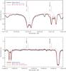 |
Fig. 1 Observed and predicted spectra of a Sun spot. Theoretical computations are shown for two magnetic field geometries: purely radial (Br,0,0) and with horizontal contribution (Br,Bm,0) (see legends on individual plots). Wavelengths are in vacuum. |
4.2. Landé factors of FeH lines
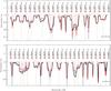 |
Fig. 2 Comparison between observed and theoretical sunspot spectra in selected regions of FeH transitions. Blue dashed line – best-fitted g-factor from Afram et al. (2008), red solid line – calculations with MZL library; both with a purely radial field of B = (2.7,0,0) kG. Red dash-dotted line – synthetic spectra accounted for the horizontal field component B = (2.5,1,0) kG (hardly seen in the figure, coincides with red solid line), brown dotted line – zero-field spectrum. Labels over lines indicate their central wavelengths, omegas of lower and upper states (in brackets), branch, and the J-number of the lower state (in brackets). Wavelengths are in vacuum. |
As noted above, Wing-Ford lines of FeH are mostly formed in intermediate Hund’s case, which makes it difficult to accurately predict Zeeman patterns of respective states. Analytically, the type of a splitting can be estimated via the analysis of spin-orbit and rotational constants Y = |Aυ| /Bυ: if Y ≫ J(J + 1) when an approximation of Hund’s case (a) is valid, and Hund’s case (b) otherwise (Herzberg 1950). Using an empirical analysis of laboratory data, Harrison & Brown (2008) determined g-factors for the upper and lower levels for a number of states with Ω = 7/2,5/2,3/2. Their Fig. 2 clearly shows a deviation from pure Hund’s cases for upper levels with J > 4.5. Almost at the same time, Afram et al. (2008) presented polynomial best-fit g-factors based on an accurate and extensive analysis of sunspot spectra. These approaches clearly illustrated the main problem: it is impossible to fit all FeH lines simultaneously with the modern theory of the intermediate Hund’s case. Instead, a good fit can be obtained only by combining theoretical and empirical approaches.
Using the MZL library and sunspot spectra we tried to compute theoretical g-factors for all lines under the condition that the resulting Zeeman patterns provide correct broadening of individual FeH lines in sunspot spectra. In general, we find that the intermediate case (with its present treatment in MZL) is a good approximation if (l – lower, u – upper states)
-
1.
Ωl = 0.5;
-
2.
Ωloru ≤ 2.5 and 3Y > J(J + 1) for the P and Q branches;
-
3.
Ωlandu = 2.5 and 5Y > J(J + 1) for the R branch.
For the rest of transitions the assumption of Hund’s case (a) for the upper level and Hund’s case (b) for lower level provide reasonable results, especially for transitions with Ωlandu = 3.5.
Figure 2 illustrates a comparison between best-fitted g-factors from Afram et al. (2008) and our calculation for some selected lines in the 9900–10 000 Å region. Note that apart from the figures shown in Afram et al. (2008), we did not make an attempt of correcting the theoretical spectra, i.e. no filling factors were applied. The model atmosphere and field intensity are the same as determined previously from the metallic line spectra. From Fig. 2 it is obvious that there is in general a good agreement between our calculation and g-factors from Afram et al. (2008). Still, the discrepancy between the two calculations is found for low omega R-branch lines like FeH 9945 Å, 9962 Å, etc., which indeed show splitting closer to pure Hund’s cases. Applying the intermediate case allows us to predict the splitting of FeH 9982 Å and the magnetic insensitive 9981 Å line. On the other hand, there is systematic difference seen for some lines (9904.98 Å, 9947 Å, etc.), where our calculations predict broader and shallow line profiles then those given in Afram et al. (2008). Even though we succeeded well enough to fit the width of the observed lines with the same field of |B| = 2.7 kG derived previously from atomic lines, this cannot be judged to be more physical though until new improvements in the theoretical description of the intermediate case will become available. In spite of atomic lines, we find little sensitivity of the FeH lines to the magnetic field geometry changing from purely radial to the additional contribution of the horizontal component. What finally matters is the total field intensity. Note, however, that it is still possible to distinguish between the dominated horizontal or radial field components via the detailed analysis of magnetically broadened FeH lines.
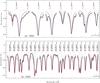 |
Fig. 3 Observed and predicted spectra of M5.5 dwarf GJ 1002 in Ti i (upper plot) and selected FeH lines (lower plot). Model parameters: Teff = 3100 K, log g = 5.0, [M/H] = 0.0, υsini = 2.5 km s-1. Observations are shown by thick solid line. Theoretical spectra were computed assuming εFe = −4.37 (red solid line) and εFe = −4.59 (blue dashed line) respectively. Wavelengths are in vacuum. |
Thus, applying different Hund’s cases based on transition quantum numbers allows us to predict the Zeeman broadening of certain FeH lines accurately and consistently (i.e. with the same field strength) with the atomic lines.
4.3. Magnetic field of selected M-dwarfs
4.3.1. General notes
A comparison of theoretical and observed sunspot spectra of FeH allows us to select lines with more or less accurately predicted Zeeman patterns and to measure magnetic fields in cooler stars. Below we present results for a few selected M-dwarfs, for which previous attempts revealed a presence of strong (up to 4 kG) effective magnetic fields (see Reiners & Basri 2007).
In cool atmospheres, the van der Waals broadening is one of the most important broadening mechanisms. For FeH, there are no theoretical or laboratory measurements of broadening constants available. We thus checked the spectra of FeH in the atmosphere of the non-magnetic M 5.5 star GJ 1002 and found that the classical van der Waals constant (see Gray 1992) used in Synmast must be increased by a factor of 3.5 to satisfactorily match the profiles of FeH lines. A model atmosphere with Teff = 3100 K, log g = 5, [M/H] = 0.0, and υsini = 2.5 km s-1 can fit strong Ti i lines in the region 10 300–10 800 Å, as shown in Fig. 3. However, using the solar abundance of iron εFe = −4.59 (εFe = log (NFe/Ntotal)) results in FeH lines that are systematically too weak. Decreasing υsini to 1 km s-1 may solve this problem, but the cores of titanium lines are then impossible to fit. Because the damping constant and log (gf)’s values for the considered Ti lines are known from more accurate calculations (which are based on observed energy levels as presented in Kurucz 1994), we used them primarily for FeH lines as indicators of accurate model parameters and υsini. The adjusted iron abundance is close to its previous solar value εFe = −4.37 (Anders & Grevesse 1989). Note that this, of course, in no way sets the correct metallicity of the star. But the lack of weakly blended Fe lines and well-known problems with continuum normalization of small spectral regions forbids more definite results. One should not forget that measuring magnetic fields mostly relies on the relative line broadening caused by Zeeman splitting, and thus the issue of metallicity is not that important in the present investigation.
There is a principle difference between modelling spectra of a sunspot and distant stars. In the former case the observer receives an intensity spectrum. Because of high spatial resolution, it is natural to assume that all individual rays of light propagate along the line-of-sight. This allows one to solve the radiative transfer problem only for one angle μ = 1. For distant stars, however, the surface integrated intensity is what is observed by our instruments. Because the geometry of the magnetic field is now a function of surface coordinates, we define the magnetic field components (radial Br, meridional Bm, azimuthal Ba) at the centre of the stellar disc. The intensities of these components are then modified according to the local μ and φ spherical angles on the stellar surface. The flux visible to the observer is obtained by angle integration of local specific intensities. For instance, assuming a non-zero Br and zero Bm and Ba, i.e. B = (Br,0,0), may correspond to the dipolar-dominated field geometry with the magnetic pole at the centre of the disc and the magnetic axis pointing along the line-of-sight.
Below we examine our approach of measuring magnetic field in atmospheres of selected M-dwarfs.
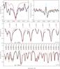 |
Fig. 4 Comparison between observed and theoretical spectra of the M 4.5 dwarf GJ 1224. Upper panel: observed and calculated spectra at the Fe i 8468 Å line (left plot) and the ratio between corresponding magnetic and non-magnetic spectra (right plot). Thick solid line – observations of GJ 1224, violet long-dashed line – observations of inactive LHS 337. Middle and lower panels: same as in Fig. 3. Model parameters: Teff = 3200 K, log g = 5.0, εFe = −4.45, υsini = 3 km s-1. Thick solid line – observations, blue dashed line – B = (2.7,0,0) kG, green dash-dotted – B = (2,0,0) kG, red solid line – B = (1.7,0,0) kG. Wavelengths are in air for upper plots and in vacuum for the middle and lower plots. |
4.3.2. GJ 1224
The source GJ 1224 is an active M 4.5 dwarf for which previous attempts to measure its magnetic field resulted in (|B| f) = 2.7 kG (Reiners & Basri 2007). An analysis of the magnetic insensitive FeH lines and Ti i 10729.3 Å line suggested Teff = 3200 K, log g = 5.0 and υsini = 3 km s-1 under assumption of solar Ti abundances. We found it necessary to slightly increase the Fe abundance to εFe = −4.45 to match the magnetically insensitive FeH lines.
The upper plot of Fig. 4 compares the observed and predicted spectra of the Fe i 8468 Å line, which was previously used by Johns-Krull & Valenti (2000) to estimate the magnetic field in a number of M-dwarfs. Here we made use of low resolution (R = 31000) Keck observations. There is a general difficulty of measuring the magnetic field strength from this line though because of heavy blending by TiO. For instance, the absorption feature in the red wing of the line (at 8468.7 Å) is actually a TiO line which thus affects the Zeeman red-shifted σ-components of the Fe i 8468 Å, whose position is then difficult to estimate with high precision. Therefore, following Johns-Krull & Valenti (2000), we tried to investigate a relative line intensity by dividing the spectra of GJ 1224 by spectra of a non-magnetic M dwarf LHS 337, which has the same or very similar spectral type. Resulting profiles are shown on the right upper panel of Fig. 4. The field of 2.7 kG can fit the slope of the red wing of the residual, but a weaker field of about 2 kG is required for the blue wing of the line. This discrepancy is likely due to a relatively low quality of the data and strong blending by TiO. In addition, this relative analysis, and especially the strength of the deep features at both sides of the line centre (see right upper plot of Fig. 4), implicitly assumes similar iron abundances for both active and inactive stars, which may not be the case.
The middle and lower plots of Fig. 4 illustrate the fit to the same set of Ti and FeH lines as performed for the non-magnetic GJ 1002 assuming different magnetic field intensities. There are several things to note. First of all, it is impossible to fit the cores of magnetic-sensitive Ti lines with any field geometry and intensity. Fields larger than 2 kG result in cores that are too wide to be observed. Inversely, using  kG allows us to obtain a reasonable fit to the width of line cores, but the predicted central depths are too strong for some lines. This behaviour is broken for the Ti 10 664.5 Å line, for which |B| = 2 kG and |B| = 1.7 kG provide a good fit, and the Ti 10 610 Å line whose core can only be described by |B| = 2 kG. Another line at 10 735 Å seems to point in the direction of |B| ≈ 2.7 kG, but the data quality at the red end of the spectra is poor and it is impossible to draw accurate conclusions.
Extending this analysis to the FeH lines brings stronger constraints for the magnetic field intensity, as shown in the lower panel of Fig. 4. In particular, magnetically sensitive lines such as FeH 9905 Å, 9906 Å, 9942 Å, and 9959 Å clearly point to the field modulus kG. That the widths of these lines are well reproduced in the sunspot spectra (see Fig. 2) allows us to consider them as important indicators of the mean field intensity. In particular, increasing |B| results in the appearance of the characteristic feature owing to the crossed σ-components of the two FeH lines at 9906 Å. Overlaid, these components give rise to the absorption feature which is not seen in the observed spectra. Consequently, weaker fields are needed to keep these lines separated. Changing the magnetic field geometry by varying the strength of the horizontal field components does not help to disable this feature: in our computations this is only possible with  kG, preferably with |B| ≈ 1.7 kG. Finally, the same conclusions are reached in the analysis of the Keck data available to us, but because of their lower resolution compared to that of CRIRES we did not include them in the plot.
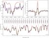 |
Fig. 5 Observed and predicted spectra of the M 4.5 dwarf YZ CMi. Model parameters: Teff = 3300 K, log g = 5.0, εFe = − 4.40, υsini = 5 km s-1. Thick solid line – observations, violet long-dashed line (upper left plot only) – observations of inactive LHS 337, green dashed – B = (0,4,0) kG, blue dash-dotted – B = (2.5,2.5,0) kG, red solid – B = (4,0,0) kG, dotted – B = (3,0,0) kG. Wavelengths are in air for the upper plot and in vacuum for the lower. |
4.3.3. YZ CMi
The source YZ CMi (GJ 285) is a particular example because of the large (|B| f) > 3.9 kG, which is the lower limit of an average field as derived by Reiners & Basri (2007). Indeed, a |B| ≈ 4 kG magnetic field seems to follow from the analysis of some atomic lines in the visual region of the high-resolution (R = 70000) Keck spectra. Figure 5 illustrates theoretical calculations for the Fe i 8468 Å line in the same manner as was done for GJ 1224 (the adopted Fe abundance is εFe = −4.40). For instance, a field of ~4 kG is needed to place the σ-components right where the TiO absorption feature is, but a somewhat weaker field of 3.5 kG is also sufficient. Unfortunately, a low signal-to-noise ratio of the observations brings only more uncertainty in the analysis and makes it difficult to chose a unique field intensity.
The predicted profiles of the FeH lines are shown in the lower plot of Fig. 5. Assuming more or less accurate continuum normalization in the region 9904–9906 Å, the fields of 4 kG provide a better fit to the line depths, but the Zeeman broadening is then too strong. The same holds true for FeH 9942 Å, 9956 Å. A weaker field of 3.5 kG with equal contributions from radial and horizontal components B = (2.5,2.5,0) kG is also a good approximation. Here again, as for the atomic lines, the low signal-to-noise ratio prevents the detailed analysis of the line core regions that carry the most important information about the magnetic field modulus. For instance, the width of the FeH lines in the 9904–9906 Å region are very well reproduced in the sunspot spectra. In this light the field of YZ CMi should be well below 4 kG. Decreasing the Fe abundance could result in a stronger field, but this is not supported by the magnetically insensitive FeH lines. Generally, the FeH lines point in the direction of a weaker field than previously reported. Less can be said about the geometry of the magnetic field, but a strong horizontal component can also be present. Higher S/N observations are strongly needed.
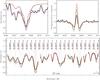 |
Fig. 6 Same as Fig. 5, but for the active M 4.5 dwarf EV Lac. Model parameters: Teff = 3400 K, log g = 5.0, εFe = − 4.40, υsini = 1 km s-1. Thick black line – observations, violet long-dashed line (upper left plot only) – observations of inactive Gl 682, green dashed – B = (0,4,0) kG, blue dash-dotted – B = (2.5,2.5,0) kG, red solid – B = (4,0,0) kG, dotted – B = (3,0,0) kG. Wavelengths are in air for the upper plot and in vacuum for the lower. |
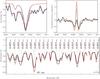 |
Fig. 7 Same as Fig. 6, but for the active M 3.5 dwarf AD Leo. Model parameters: Teff = 3400 K, log g = 5.0, εFe = −4.50, υsini = 3 km s-1. Thick black line – observations, violet long-dashed line (upper left plot only) – observations of inactive Gl 682, green dashed – B = (1.7,1.7,0) kG, blue dash-dotted – B = (2,0,0) kG, brawn dotted – B = (2.5,0,0) kG, red solid – B = (2.9,0,0) kG. Wavelengths are in air for the upper plot and in vacuum for the lower. |
4.3.4. EV Lac
The dwarf EV Lac (GJ 873) is another object with a strong field that was previously reported (see Johns-Krull & Valenti 2000; Reiners & Basri 2007). Again, the relatively low quality (R = 31000) of the data makes it difficult to conclude on the field strength from the analysis of the Fe i 8468 Å line, as illustrated in Fig. 6, but at least its blue wing is unaffected by instrumental effect. As for YZ CMi, a ~4 kG magnetic field can still result in the position of a red-shifted σ-component in the line, as demonstrated by the theoretical calculation, but a field of 3.5 kG seems to better match the position of the blue-shifted σ-component. Taking into account that a 3 kG field provides probably the worst match, the actual mean magnetic field is likely between 3 and 4 kG. A sharp core of the Fe line itself (as a result of low-resolution observations) renders any quantitative measurement of the magnetic field redundant. Again, similar to the case of YZ CMi, the FeH lines (mostly those around 9906 Å) point to weaker fields of about 3–3.5 kG. We are thus forced to conclude that spectra of a much better quality are highly required for more definite results. The model parameters we used are: Teff = 3400 K, log g = 5.0, [M/H] = 0.0, υsini = 1 km s-1, iron abundance εFe = −4.40.
4.3.5. AD Leo
The source AD Leo (GJ 388) is the famous flare star and the last target in our sample. At first, Johns-Krull & Valenti (2000) reported a field of (|B| f) ~ 3.3 kG, which was then slightly decreased to 2.9 kG in Reiners & Basri (2007). Figure 7 illustrates the fit to the FeH and Fe i 8468 Å lines under the assumption of different magnetic field intensity. The model parameters we used are: Teff = 3400 K, log g = 5.0, εFe = − 4.50, υsini = 3 km s-1. Note that it is impossible to match the width and depth of magnetic insensitive FeH lines with any combination of υsini, Teff, and Fe abundances unless one assumes a somewhat higher spectral resolution. We found that R ≈ 45000 is required instead of R = 30000. We adopt this higher effective resolving power, which can be caused by the better image quality at a seeing of the order of 0.8′′. This is likely to provide a better effective resolution than the much wider slit size. The profiles of the FeH lines suggest |B| = 2 − 2.5 kG on average, but with anomalously narrow line cores, whose fit would require an even lower field modulus (again, with FeH 9906 Å definitely pointing to |B| ~ 2 kG). It is hard to conclude precisely about the field intensity from the Fe i 8468 Å line, as seen from the upper panel of Fig. 7.
5. Discussion
In spite of recent progress in understanding and modelling the Zeeman effect in cool spectra of FeH transitions, there are still problems which limit the precise measurements of the stellar magnetic fields.
The approximate treatment of the intermediate Hund’s case is the main source of uncertainties in the analysis of FeH lines. It was noted already in Afram et al. (2008) and confirmed in the present calculations that the effective Hamiltonian of the intermediate case seems to miss an important term, which results in the underestimation of line broadening as seen from theoretical profiles of magnetically sensitive lines. It can only describe the Zeeman pattern of states with lower Ω numbers, and fails for the great majority of lines. This unknown perturbation still awaits its explanation. Nevertheless, we show that a semi-empirical approach of using different Hund’s cases for different states depending on their quantum numbers can very well reproduce profiles of many FeH lines in the Wing-Ford band. This allows us to select lines with correctly reproduced Zeeman patterns and to use them as probes of the magnetic fields in other stars by direct spectra synthesis.
In our semi-empirical approach we used a sunspot spectrum to adjust theoretical g-factors of FeH lines. Because the properties of the plasma in a cool sunspot region are less accurately known than the surrounding “standard” atmosphere of the Sun, this is where in principle some systematics could be introduced in the resulting values of g-factors. However, these effects are minimized because a) the magnetic field inside the spot and plasma properties are found from the independent diagnostics as provided by atomic lines, b) the magnetic insensitive FeH lines are accurately fitted, and c) we obtained a self-consistent fit to FeH and atomic lines using the same field strength, abundances, and model atmosphere. In addition, we tried for the FeH lines to fit not only the line broadening but also the Zeeman pattern (i.e. shapes of theoretical and observed FeH lines).
Owing to the high J-numbers, it is impossible to see individual Zeeman components of molecular lines because they are smeared out and result only in the line broadening (a single FeH line can give rise to up to few tens and even hundreds of π- and σ-components). To accurately measure this broadening, high resolution and high S/N (preferably >100) observations are desired. In this regard, and also because of our accurate knowledge of g-factors, atomic lines are superior probes of magnetic fields with intensities higher than a few kG. For weaker fields, FeH lines are a better choice, but, once again, under the condition that their splitting is well understood.
For two stars, YZ CMi and EV Lac, we confirm the presence of strong magnetic fields from the analysis of FeH spectra, but their intensity appears to be systematically lower than previously reported (see Fig. 5, for example). The forest of strong TiO features limits an accurate analysis of (ideally) good indicators such as Fe i 8466 Å line. Furthermore, for both stars the low signal-to-noise ratio of the data forbids an accurate fitting of the FeH lines. What remains are the widths of individual lines, which are very well fitted in the sunspot spectra, providing in this way the more or less solid ground for the magnetic field analysis. All these lines point to weaker fields, probably not more than 3.5 kG. Even though a field of 4 kG with a dominating horizontal component gives line depths similar to those of 3.5 kG, the line widths still appear to be wider than observed. This is an expected result because the choice of the field geometry (with the same intensity) does not affect the width of the line. This is another strong reason to call for more precise observations.
The analysis of the FeH spectra of another active M 3.5 star AD Leo also points to a weaker (by 15–30%) mean magnetic field than previously reported. For instance, from the analysis of an infrared Na i 2208.4 Å line Kochukhov et al. (2009) find ∑ (|B| f) = 4.5 kG and ∑ (|B| f) = 3.2 kG for YZ CMi and AD Leo respectively. In the former case the field is 27% larger than those derived in Johns-Krull & Valenti (2000), which can be a result of different probes (Fe i 8468 Å and Na i 2208.4 Å) and techniques. This discrepancy between the magnetic fields inferred from the atomic and molecular diagnostics is unlikely to be caused by the different depths of line formation that might be modelled in model atmospheres with different accuracy. This is because a good fit to both atomic Ti i and FeH lines is obtained for the non-magnetic GJ 1002, which significantly reduces (but not necessary completely excludes!) any possible model atmosphere effect. More intense investigation is clearly needed and should involve simultaneouse atomic and molecular probes for a stronger confirmation of our results.
Last but not least, the parameters of the FeH lines are derived from theoretical computations and thus may suffer from systematic inaccuracies. In this study we tried to adjust the parameters of some FeH with the spectra of non-magnetic stars, but this needs more thorough investigation (see Wende et al. 2010). Note again that the adjustment of the Einstein A-coefficients of some FeH lines from the original line list has very little effect on the measured magnetic field intensities. This is because the latter relies on the line broadening due to Zeeman splitting and not on the line depth, which is modified by corrected A-coefficients. The inferred iron abundance is different in some cases from its recent solar value. This can be the result of using precalculated model atmospheres with fixed effective temperatures: to fit the spectrum of a particular star we always used a model atmosphere from the grid whose Teff(model) is close but can still be different from the Teff(star). In cool atmospheres parameters such as Teff and the Fe abundance are degenerate, i.e. the spectra of FeH react the same way if one changes any of these parameters. Thus, the solution is always not unique in this particular parameter’s space. Nevertheless, an uncertainty of about 0.2 dex in Fe abundance (as in the case of our reference non-magnetic star GJ 1002), and any uncertainty in A-coefficients, would mostly change the line depths, and therefore we expect them to have little effect on the inferred magnetic field intensity, because this relies on the line broadening due to Zeeman splitting.
For GJ 1224, the splitting pattern of FeH lines points to the field intensity which is, at maximum, 1 kG less than the one reported in Reiners & Basri (2007), which was (|B| f) = 2.7 kG. A 2.7 kG field is probably too high as demonstrated by FeH lines (see Fig. 4). In particular, the separation of two FeH lines 9905 Å and 9906 Å appears to be a good indicator of the mean field intensity. As noted above, with increasing field strength over ≈2 kG, these lines tend to produce a characteristic feature, which is not observed. Another interesting behaviour is demonstrated by the Ti lines red-ward of 1 μm. The central depths of three of them (10 399.6 Å, 10 498.9 Å, 10 587.5 Å) require a field around 2.7 kG, but their widths, in contrast, point to a much weaker field. In addition, Ti i 10 610 Å, 10 664.5 Å are well reproduced with ≈ 2 kG field. That these lines are nicely fitted in the spectra of the non-magnetic GJ 1002 possibly excludes systematic inaccuracies in spectra processing, because both spectra were observed with the same instrument and processed in the same way.
Atmospheric parameters of investigated M-dwarfs.
There is, however, a consideration that relies on different dates of spectra taken for GJ 1224. Thus, if one assumes a presence of a magnetic spot(s) on the surface of the star and if the star is hosting a strong field, and the rest of the surface has a somewhat weaker field, then a different field intensity observed in different spectral regions and at different rotational phases is indeed naturally expected. The presence of wide regions with strong magnetic fields was confirmed for some M-dwarfs, but the field topology of the majority of them is found to be dominated by the poloidal component, which indicates rather homogeneous magnetic fields (see Donati et al. 2006, 2008; Morin et al. 2008). The complete characterization of the magnetic field in active M-dwarfs via the phase-resolved observations in all Stokes parameters are thus of particular interest, though it is a very challenging task even for modern instruments.
In this work we attempted to measure a mean surface magnetic field. This may not correspond to a real picture because, as stated above, the magnetic field of M-dwarfs is likely to be concentrated in magnetically active areas (spots) similar to what is observed in the solar atmosphere. Thus, a mean surface field can be represented by (at least) two components: a strong field inside a spot/spots and a much weaker component of a surrounding surface (which can be zero as well). To account for this geometrical consideration the corresponding filling factors f (i.e. free parameters that describe the relative size of magnetic regions characterized by a given magnetic field modulus) must be applied. The more accurate way to account for the complex magnetic field geometry without the need of filling factors would be the analysis of polarized radiation in individual lines. However, as stated above, this is extremely difficult or almost impossible to do with the current instrumentation. Again, similar to the Sun, the temperature inside these spot(s) may also be lower than the surrounding plasma. This will be investigated in our future works, also with data of better quality.
Table 1 gathers the main results of the present study. An average surface magnetic field resulting from the analysis of atomic and FeH lines are shown separately. A large scatter resulting from the analysis of the Fe i 8468 Å line is due to the uncertainties of fitting blue and red wings of the flux ratio (see, for instance, Figs. 4 and 6), which seem to require different |B| .
6. Summary
In this study we made an attempt of using up-to-date knowledge of molecular Zeeman effect, modern software for the magnetic spectra synthesis, and molecular lines data to develop an approach of modelling the Zeeman splitting in FeH lines of Wing-Ford F4Δ − X4Δ band. This approach was then applied to measure magnetic fields in selected M-dwarfs for which observations in both atomic and FeH lines are available. The main results of the present work can be summarized as follows:
-
1.
Our results of the magnetic field strengths derived fromFeH lines are 15–30% lower thanresults presented in Reiners & Basri (2007),which are based on atomic line analysis scaled from Johns-Krull& Valenti (2000).
-
2.
We confirm a strong magnetic field found in YZ CMi, EV Lac, and AD Leo but with an intensity which is likely 500 G (or more) weaker. Unfortunately, the poor quality of the data forbids a more quantitative conclusions.
-
3.
An analysis of atomic and FeH lines in spectra of GJ 1224 points in the direction of 1.7–2 kG averaged magnetic field, which is lower than 2.7 kG previously reported (Reiners & Basri 2007).
-
4.
The estimates of the magnetic field modulus from the Fe i 8468 Å line seem to be systematically higher than those from FeH lines. This, however, should be taken with caution because of unknowns associated with the quality of the data and atmospheric parameters used.
-
5.
With routines provided by Molecular Zeeman Library we developed an algorithm for calculating Landé g-factors of FeH states: the choice of the Hund’s cases (a), (b) or intermediate follows from the consideration of quantum numbers of individual states. The test computations of the sunspot spectra showed a good agreement with observations and with calculations based on the best-fit g-factors from Afram et al. (2008).
-
6.
To distinguish between different magnetic field geometries, higher quality observations are required for the analysis of FeH spectra (S/N > 100).
-
7.
To exclude possible selection effects caused by the variable field associated with the magnetic spot(s), and to provide a complete characterization of the magnetic field intensity and geometry, time-resolved observations are highly desired. These observations, which would ideally provide spectra in all four Stokes parameters as well, remain highly difficult even for the brightest M-dwarfs because they require many hours of signal integration time to achieve the desired S/N even with modern astronomical instrumentation.
Acknowledgments
We thank Dr. Bernard Leroy for his kind advice and help with the MZL routines. This work was supported by the following grants: Deutsche Forschungsgemeinschaft (DFG) Research Grant RE1664/7-1 to D.S. and Deutsche Forschungsgemeinschaft under DFG RE 1664/4-1 and NSF grant AST07-08074 to
A.S. S.W. acknowledges financial support from the DFG Research Training Group GrK – 1351 “Extrasolar Planets and their host stars”. O.K. is a Royal Swedish Academy of Sciences Research Fellow supported by grants from the Knut and Alice Wallenberg Foundation and the Swedish Research Council. We also acknowledge the use of electronic databases (VALD, SIMBAD, NASA’s ADS). This research has made use of the Molecular Zeeman Library (Leroy 2004).
References
- Afram, N., Berdyugina, S. V., Fluri, D. M., et al. 2007, A&A, 473, L1 [NASA ADS] [CrossRef] [EDP Sciences] [Google Scholar]
- Afram, N., Berdyugina, S. V., Fluri, D. M., Solanki, S. K., & Lagg, A. 2008, A&A, 482, 387 [NASA ADS] [CrossRef] [EDP Sciences] [Google Scholar]
- Anders, E., & Grevesse, N. 1989, Geochim. Cosmochim. Acta, 53, 197 [Google Scholar]
- Asensio Ramos, A., & Trujillo Bueno, J. 2006, ApJ, 636, 548 [NASA ADS] [CrossRef] [Google Scholar]
- Asplund, M., Grevesse, N., & Sauval, A. J. 2005, in Cosmic Abundances as Records of Stellar Evolution and Nucleosynthesis, ed. T. G. Barnes III, & F. N. Bash, ASP Conf. Ser., 336, 25 [Google Scholar]
- Berdyugina, S. V. 2005, Liv. Rev. Sol. Phys., 2, 8 [Google Scholar]
- Berdyugina, S. V., & Solanki, S. K. 2002, A&A, 385, 701 [NASA ADS] [CrossRef] [EDP Sciences] [Google Scholar]
- Donati, J.-F., & Landstreet, J. D. 2009, ARA&A, 47, 333 [NASA ADS] [CrossRef] [MathSciNet] [Google Scholar]
- Donati, J.-F., Morin, J., Petit, P., et al. 2008, MNRAS, 390, 545 [NASA ADS] [CrossRef] [Google Scholar]
- Donati, J.-F., Forveille, T., Cameron-Collier, A., et al. 2006, Science, 311, 633 [NASA ADS] [CrossRef] [PubMed] [Google Scholar]
- Dulick, M., Bauschlicher, Jr., C. W., Burrows, A., et al., 2003, ApJ, 594, 651 [NASA ADS] [CrossRef] [Google Scholar]
- Gray D. F. 1992, The Observation and Analysis of Stellar Photospheres (Cambridge University Press) [Google Scholar]
- Gustafsson, B., Edvardsson, B., Eriksson, K., et al. 2008, A&A, 486, 951 [NASA ADS] [CrossRef] [EDP Sciences] [Google Scholar]
- Harrison, J. J., & Brown, J. M. 2008, ApJ, 686, 1426 [NASA ADS] [CrossRef] [Google Scholar]
- Herzberg, G. 1950 Molecular Spectra and Molecular Structure. I. Spectra of Diatomic Molecules, D. van Nostrand, Florida [Google Scholar]
- Johns-Krull, C. M. 2007, ApJ, 664, 975 [NASA ADS] [CrossRef] [Google Scholar]
- Johns-Krull, C. M., & Valenti, J. A. 1996, ApJ, 459, L95 [NASA ADS] [CrossRef] [Google Scholar]
- Johns-Krull, C. M., & Valenti, J. A. 2000, Stellar Clusters and Associations: Convection, Rotation, and Dynamos, ed. R. Pallavicini, G. Micela, & S. Sciortino, ASP Conf. Ser., 198, 371 [Google Scholar]
- Kochukhov, O., Heiter, U., Piskunov, N., et al. 2009, AIP Conf. Ser., 1094, 124 [Google Scholar]
- Kochukhov, O. 2007, in Physics of Magnetic Stars, ed. D. O. Kudryavtsev, & I. I. Romanyuk, Nizhnij Arkhyz., 109 [Google Scholar]
- Kupka, F., Piskunov, N., Ryabchikova, T. A., Stempels, H. C., & Weiss, W. W. 1999, A&AS, 138, 119 [NASA ADS] [CrossRef] [EDP Sciences] [MathSciNet] [PubMed] [Google Scholar]
- Kurucz, R. L. 1994, Kurucz CD-ROM 20-22, Cambridge, SAO [Google Scholar]
- Landstreet, J. D. 2001, in Magnetic Fields Across Hertzsprung-Russell Diagram, ed. G. Mathys, S. K. Solanki, & D. T. Wickramasinghe, ASP Conf. Ser., 248, 277 [Google Scholar]
- Landstreet, J. D. 1992, A&AR, 4, 35 [Google Scholar]
- Leroy, B. 2004, Molecular Zeeman Library Reference Manual, http://bass2000.obspm.fr/mzl/download/mzl-ref.pdf [Google Scholar]
- Morin, J., Donati, J.-F., Petit, P., et al. 2008, MNRAS, 390, 567 [NASA ADS] [CrossRef] [MathSciNet] [Google Scholar]
- Piskunov, N. 1999, Astrophys. Space Sci. Library, 243, 515 [Google Scholar]
- Piskunov, N. E., Kupka, F., Ryabchikova, T. A., Weiss, W. W., & Jeffery, C. S. 1995, A&AS, 112, 525 [Google Scholar]
- Reiners, A., & Basri, G. 2006, ApJ, 644, 497 [NASA ADS] [CrossRef] [Google Scholar]
- Reiners, A., & Basri, G. 2007, ApJ, 656, 1121 [NASA ADS] [CrossRef] [Google Scholar]
- Reiners, A., & Basri, G. 2009, A&A, 496, 787 [NASA ADS] [CrossRef] [EDP Sciences] [Google Scholar]
- Reiners, A., & Basri, G. 2010, ApJ, 710, 924 [NASA ADS] [CrossRef] [Google Scholar]
- Reiners, A., Basri, G., & Browning, M. 2009, ApJ, 692, 538 [NASA ADS] [CrossRef] [Google Scholar]
- Saar, S. H. 2001, 11th Cambridge Workshop on Cool Stars, Stellar Systems and the Sun, ed. R. J. Garcia Lopez, R. Rebolo, & M. R. Zapaterio Osorio, ASP Conf. Ser., 223, 292 [Google Scholar]
- Schadee, A. 1978, J. Quant. Spec. Radiat. Transf., 19, 517 [Google Scholar]
- Valenti, J. A., Johns-Krull, C. M., & Piskunov, N. E. 2001, 11th Cambridge Workshop on Cool Stars, Stellar Systems and the Sun, ed. R. J. Garcia Lopez, R. Rebolo, & M. R. Zapaterio Osorio, ASP Conf. Ser., 223, 1579 [Google Scholar]
- Wallace, L., Livingston, W. C., Bernath, P. F., & Ram, R. S. 1998, An Atlas of the Sunspot Umbral Spectrum in the Red and Infrared from 8900 to 10 050 cm-1 (6642 to 11 230 Å) (NOAO) [Google Scholar]
- Wende, S., Reiners, A., Seifahrt, A., & Bernath, P. F. 2010, A&A, accepted, [arXiv:1007.4116] [Google Scholar]
All Tables
All Figures
|
Fig. 1 Observed and predicted spectra of a Sun spot. Theoretical computations are shown for two magnetic field geometries: purely radial (Br,0,0) and with horizontal contribution (Br,Bm,0) (see legends on individual plots). Wavelengths are in vacuum. |
| In the text | |
|
Fig. 2 Comparison between observed and theoretical sunspot spectra in selected regions of FeH transitions. Blue dashed line – best-fitted g-factor from Afram et al. (2008), red solid line – calculations with MZL library; both with a purely radial field of B = (2.7,0,0) kG. Red dash-dotted line – synthetic spectra accounted for the horizontal field component B = (2.5,1,0) kG (hardly seen in the figure, coincides with red solid line), brown dotted line – zero-field spectrum. Labels over lines indicate their central wavelengths, omegas of lower and upper states (in brackets), branch, and the J-number of the lower state (in brackets). Wavelengths are in vacuum. |
| In the text | |
|
Fig. 3 Observed and predicted spectra of M5.5 dwarf GJ 1002 in Ti i (upper plot) and selected FeH lines (lower plot). Model parameters: Teff = 3100 K, log g = 5.0, [M/H] = 0.0, υsini = 2.5 km s-1. Observations are shown by thick solid line. Theoretical spectra were computed assuming εFe = −4.37 (red solid line) and εFe = −4.59 (blue dashed line) respectively. Wavelengths are in vacuum. |
| In the text | |
|
Fig. 4 Comparison between observed and theoretical spectra of the M 4.5 dwarf GJ 1224. Upper panel: observed and calculated spectra at the Fe i 8468 Å line (left plot) and the ratio between corresponding magnetic and non-magnetic spectra (right plot). Thick solid line – observations of GJ 1224, violet long-dashed line – observations of inactive LHS 337. Middle and lower panels: same as in Fig. 3. Model parameters: Teff = 3200 K, log g = 5.0, εFe = −4.45, υsini = 3 km s-1. Thick solid line – observations, blue dashed line – B = (2.7,0,0) kG, green dash-dotted – B = (2,0,0) kG, red solid line – B = (1.7,0,0) kG. Wavelengths are in air for upper plots and in vacuum for the middle and lower plots. |
| In the text | |
|
Fig. 5 Observed and predicted spectra of the M 4.5 dwarf YZ CMi. Model parameters: Teff = 3300 K, log g = 5.0, εFe = − 4.40, υsini = 5 km s-1. Thick solid line – observations, violet long-dashed line (upper left plot only) – observations of inactive LHS 337, green dashed – B = (0,4,0) kG, blue dash-dotted – B = (2.5,2.5,0) kG, red solid – B = (4,0,0) kG, dotted – B = (3,0,0) kG. Wavelengths are in air for the upper plot and in vacuum for the lower. |
| In the text | |
|
Fig. 6 Same as Fig. 5, but for the active M 4.5 dwarf EV Lac. Model parameters: Teff = 3400 K, log g = 5.0, εFe = − 4.40, υsini = 1 km s-1. Thick black line – observations, violet long-dashed line (upper left plot only) – observations of inactive Gl 682, green dashed – B = (0,4,0) kG, blue dash-dotted – B = (2.5,2.5,0) kG, red solid – B = (4,0,0) kG, dotted – B = (3,0,0) kG. Wavelengths are in air for the upper plot and in vacuum for the lower. |
| In the text | |
|
Fig. 7 Same as Fig. 6, but for the active M 3.5 dwarf AD Leo. Model parameters: Teff = 3400 K, log g = 5.0, εFe = −4.50, υsini = 3 km s-1. Thick black line – observations, violet long-dashed line (upper left plot only) – observations of inactive Gl 682, green dashed – B = (1.7,1.7,0) kG, blue dash-dotted – B = (2,0,0) kG, brawn dotted – B = (2.5,0,0) kG, red solid – B = (2.9,0,0) kG. Wavelengths are in air for the upper plot and in vacuum for the lower. |
| In the text | |
Current usage metrics show cumulative count of Article Views (full-text article views including HTML views, PDF and ePub downloads, according to the available data) and Abstracts Views on Vision4Press platform.
Data correspond to usage on the plateform after 2015. The current usage metrics is available 48-96 hours after online publication and is updated daily on week days.
Initial download of the metrics may take a while.