| Issue |
A&A
Volume 523, November-December 2010
|
|
|---|---|---|
| Article Number | A52 | |
| Number of page(s) | 7 | |
| Section | Planets and planetary systems | |
| DOI | https://doi.org/10.1051/0004-6361/201015052 | |
| Published online | 16 November 2010 | |
The Doppler shadow of WASP-3b
A tomographic analysis of Rossiter-McLaughlin observations
1
School of Physics & Astronomy, University of St
Andrews,
North Haugh, St Andrews,
Fife
KY16 9SS,
UK
e-mail: This email address is being protected from spambots. You need JavaScript enabled to view it.
2
Astrophysics Research Centre, School of Mathematics &
Physics, Queen’s University, University Road, Belfast
BT7 1NN,
UK
3
Department of Physics, University of Oxford,
Denys Wilkinson Building, Keble
Road, Oxford
OX1 3RH,
UK
4
Observatoire de l’Université de Genève,
Chemin des Maillettes
51, 1290
Sauverny,
Switzerland
5
Institut d’Astrophysique de Paris, UMR7095 CNRS, Université Pierre
& Marie Curie, 98bis Bd
Arago, 75014
Paris,
France
6
Laboratoire d’Astrophysique de Marseille,
BP 8,
13376
Marseille, Cedex 12,
France
7
Isaac Newton Group of Telescopes, Apartado de Correos 321, 38700
Santa Cruz de la Palma, Tenerife, Spain
Received:
26
May
2010
Accepted:
16
August
2010
Abstract
Context. Hot-Jupiter planets must form at large separations from their host stars where the temperatures are cool enough for their cores to condense. They then migrate inwards to their current observed orbital separations. Different theories of how this migration occurs lead to varying distributions of orbital eccentricity and the alignment between the rotation axis of the star and the orbital axis of the planet.
Aims. The spin-orbit alignment of a transiting system is revealed via the Rossiter-McLaughlin effect, which is the anomaly present in the radial velocity measurements of the rotating star during transit due to the planet blocking some of the starlight. In this paper we aim to measure the spin-orbit alignment of the WASP-3 system via a new way of analysing the Rossiter-McLaughlin observations.
Methods. We apply a new tomographic method for analysing the time variable asymmetry of stellar line profiles caused by the Rossiter-McLaughlin effect. This new method eliminates the systematic error inherent in previous methods used to analyse the effect.
Results. We find a value for the projected stellar spin rate of
v sin i = 13.9 ± 0.03 km s-1 which is in
agreement with previous measurements but has a much higher precision. The system is found
to be well aligned, with  ° which
favours an evolutionary history for WASP-3b involving migration through tidal interactions
with a protoplanetary disc. From comparison with isochrones we put an upper limit on the
age of the star of 2 Gyr.
° which
favours an evolutionary history for WASP-3b involving migration through tidal interactions
with a protoplanetary disc. From comparison with isochrones we put an upper limit on the
age of the star of 2 Gyr.
Key words: planetary systems / line: profiles / techniques: spectroscopic / eclipses / stars: individual: WASP-3b
© ESO, 2010
1. Introduction
Since the confirmation in 1995 of the first extrasolar planet orbiting a main sequence star (Mayor & Queloz 1995) it has become evident that gas-giant planets with orbital separations smaller than that of Mercury are quite common. In fact, these Hot Jupiters account for around 20% of the approximately 4501 exoplanets discovered to date, though their current prevalence in transit searches is mostly due to observational bias and recent results from the Kepler Mission suggest that the majority of exoplanets are of lower mass (Borucki & for the Kepler Team 2010). It has been shown that these planets must form farther out, beyond what is known as the “snow line” (Sasselov & Lecar 2000), and then migrate inwards to their current locations (Lin et al. 1996). If this is the case then through what process does this migration occur and how can we gain information on this from current observations?
There are three main competing theories of Hot-Jupiter migration. The first states that migration occurs due to tidal interactions between the planet and the protoplanetary disc causing some of the planet’s angular momentum to be lost to the disc (Goldreich & Tremaine 1980; Nelson et al. 2000). The second proposes that gravitational scattering between multiple planets in a system can cause one planet to migrate inwards at the expense of the other being shot out of the system (Weidenschilling & Marzari 1996; Chatterjee et al. 2008; Jurić & Tremaine 2008).
These separate scenarios should lead to quite different post-migration states. Tidal interactions between the planet and protoplanetary disc will result in a system where the orbital axis of the planet is well aligned with the rotation axis of the host star. It would also lead to highly circularised orbits. The planet-planet scattering process on the other hand would result in planets which have larger orbital eccentricities and are not necessarily well aligned (Weidenschilling & Marzari 1996).
The third proposed process involved in Hot Jupiter migration is the Kozai mechanism. It involves oscillations between the spin-orbit alignment angle and the orbital eccentricity of the planet due to the presence of another (outer) planet in the system or a binary companion of the host star (Kozai 1962; Wu & Murray 2003; Fabrycky & Tremaine 2007). During these oscillations the value  is conserved, where e is the planet’s orbital eccentricity and i is its inclination to the orbital plane of the other objects. Nagasawa et al. (2008) suggested a combination of all three processes could be responsible for the migration of Hot Jupiters.
Measuring the alignments of the known Hot-Jupiter systems helps shed some light on the migration process and refine models of system evolution. The misalignment angle λ between the planet’s orbital axis and the rotation axis of the host star can be determined via the Rossiter-McLaughlin effect (Rossiter 1924; McLaughlin 1924). This is the radial velocity anomaly observed during transit due to the planet blocking some of the starlight. A planet in a prograde orbit would first block some blue-shifted light, from the half of the star which is rotating towards us, causing an anomalous red-shift in the star’s radial velocity. Then once it has crossed the stellar rotation axis it will block light from the receding half of the disc causing an anomalous blue-shift. The form of this radial velocity anomaly allows us to measure the projected stellar rotation rate and the spin-orbit misalignment angle (Gaudi & Winn 2007).
Ohta et al. (2005) and Giménez (2006) derived detailed expressions for measuring the anomalous shift in the line centroid during transit. Using the radial velocity shift to determine the parameters related to the Rossiter-McLaughlin effect can be a problem when the spectrograph can resolve the stellar line profile. The data pipelines for instruments such as SOPHIE and HARPS calculate RVs by fitting a Gaussian profile to the cross-correlation function (CCF) in order to measure the shift in line centroid. However, as the planet is blocking some of the light from the star this shows up on the line profile as a travelling “bump” of width equal to that of the local non-rotating line profile. This means that the CCF is now asymmetric and time-varying during transit, introducing a systematic deviation to measurements of the radial velocity (Winn et al. 2005). This error becomes greater for more rapidly rotating host stars as their line profiles exhibit higher degrees of rotational broadening (Hirano et al. 2010).
In more recent studies Winn et al. (2005, 2006, 2007) tried to account for this by building models of the out of transit line profile and the light blocked by the planet. They included these into their analysis of the line-spread function and produced semi-empirical corrections to the model radial velocities. However, their method does not account for the problem entirely as their analysis of HD 189733b shows a clear pattern of correlated residuals in the radial velocities during transit (Winn et al. 2006). A similar pattern in the radial velocity residuals of HD 189733b was found by Triaud et al. (2009) who discuss their cause in detail. Simpson et al. (2010) also found a similar correlation pattern when analysing the WASP-3 system using the expressions from Ohta et al. (2005) with the corrections developed by Hirano et al. (2010). In order to eliminate the need for empirical corrections Collier Cameron et al. (2010a) developed a new method that involves decomposing the CCF profile into its various components, namely the limb-darkened rotation profile, gaussian average line profile and the travelling signature caused by the transiting planet.
To gain information on the distribution of spin-orbit misalignment angles, the WASP (Wide Angle Search for Planets) consortium has been performing follow-up spectrographic observations of the transits of the known WASP planets. Observations have been made using the HARPS spectrograph on the ESO 3.6 m telescope at La Silla and the SOPHIE spectrograph on the 1.93 m telescope at the Observatoire de Haute-Provence. WASP-3b is the third planet discovered through the SuperWASP project (Pollacco et al. 2008). It is a Hot Jupiter orbiting a main sequence star of spectral type F7-8V.
In this study we implement the method of Collier Cameron et al. (2010a) to remove the inherent error present in the Gaussian-fitting method by instead focusing on the light removed by the planet. We model all the components of the line-spread function and fit to spectral observations of WASP-3b in order to track the trajectory of the missing light component as it crosses the line profile during transit. A model of the out-of-transit profile is subtracted from the data leaving only the signature of the blocked light. The trajectory of this feature is used to derive values for the projected stellar rotation rate, the impact parameter and the spin-orbit misalignment.
This method does not rely on high precision radial velocity measurements, making it uniquely useful for detecting planets orbiting rapid-rotating early-type stars (Collier Cameron et al. 2010b). Many of these stars which have reliable photometric data have been dropped from radial velocity follow-up observations due to their rotation rate and line-poor spectra.
2. Observations and analysis
We reanalyse data presented in Simpson et al. (2010) who used the SOPHIE echelle spectrograph (Bouchy et al. 2009) on the 1.93 m telescope at the Observatoire de Haute-Provence to take 26 observations before, during and after the transit of WASP-3b on the night of September 30th 2008. A major advantage of this new method is that it does not require high precision radial velocity measurements, therefore the spectrograph was used in high efficiency mode (R = 40000). The exposure times for the observations ranged from 300 − 1800 s to ensure a constant signal-to-noise ration of 35. In total 137 min of observations were taken during transit and 130 min out of transit. CCFs were computed using the automated SOPHIE data-reduction pipeline which is adapted from the HARPS data-reduction software. WASP-3 is of spectral type F7-8V, so the weighted mask function used for the cross-correlation was for a G2V star as this was the closest type offered by the pipeline. For a more detailed explanation of the observations and data reduction procedure see Simpson et al. (2010).
2.1. Modelling the observations
The following sections outline the key points of the new method used to analyse the CCF data. The modelling process is described in detail by Collier Cameron et al. (2010a).
First we need to build a model of the out-of-transit CCF. This is done by convolving a Gaussian representing the the local line profile at any point on the surface of the star with a limb-darkened rotation profile. For the local line profile we use  (1)For the limb-darkened rotation profile we use the equation
  (2)assuming a linear limb-darkening model where u is the limb-darkening coefficient and − 1 < x < 1. We adopted a value of u = 0.69 taken from the Claret (2004) tables for the g′ filter. This value corresponds to a star with Teff = 6500 K, log g∗ = 4.5 and [ M / H ] = 0 which best describe the values for WASP-3 calculated through analysis of the SOPHIE spectra and presented in the discovery paper (Teff = 6400 ± 100 K, log g∗ = 4.5 ± 0.05).
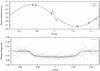 |
Fig. 1 Upper panel: phase-folded plot of the 6 out-of-transit radial velocity measurements which are not affected by any time-varying asymmetry of the line-profile. The out-of-transit RV fit was calculated using the velocity semi-amplitude, orbital eccentricity, arguement of periastron and true anomaly. The position of the planet over the stellar disc, ratio of star/planet radii, impact parameter and non-linear limb darkening coefficients were used to model the RM anomaly during transit. Lower panel: phase-folded plot of all 8 sets of photometric data analysed in this study. |
The convolution of these two functions is given by  (3)which is calculated by numerical integration. We need to shift the model CCF to account for the fact that the CCFs are computed in the velocity frame of the solar system barycentre. To do this we compute
  (4)where vij is the velocity of pixel i in the barycentric frame, νj is the true anomaly at the time of the jth observation, ω is the argument of periastron, e is the orbital eccentricity, K is the radial velocity amplitude and γ is the systemic centre-of-mass velocity.
At any moment in time the position of the planet on the plane of the sky is given by the co-ordinates 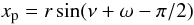 (5)
(5) (6)where r is the instantaneous distance of the planet from the star and i is the inclination of the orbital axis to the line-of-sight. The perpendicular distance of the planet from the stellar rotation axis in units of R∗ is now
 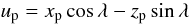 (7)where λ = φspin − φorbit and φ is the position angle in the plane of the sky (Winn et al. 2005). Combining the model out-of-transit CCF with the model of the missing starlight gives us
 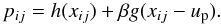 (8)Here the term h(xij) is the model of the out-of-transit stellar CCF. The term βg(xij − up) represents the travelling Gaussian signature caused by the missing starlight, where β is the fraction of starlight blocked by the planet during the total part of the eclipse. Figure 2 shows the original CCFs and the resulting residuals when first the model CCFs h(xij) are subtracted off leaving the signature of the missing starlight and secondly the overall residuals when the complete model pij is subtracted.
2.2. Fitting the model
In order to orthogonalise the data and the model we subtract their optimal mean values using inverse-variance weights  :
:
The goodness of fit of the model to the observed data is then calculated using the χ2 statistic 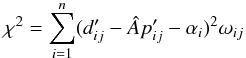 (9)where αi is the optimal average of the residual spectra and  is a multiplicative constant calculated via optimal scaling.
The spectral resolving power of the SOPHIE spectrograph is R = 75000 which gives a velocity resolution of 4 km s-1. However, the CCFs are produced with velocity increments of 0.5 km s-1 meaning that the errors on the data from neighbouring pixels are correlated. In order to make sure our data points were statistically independent we binned them by a factor of 8 before computing χ2.
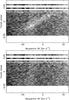 |
Fig. 2 Top: residual map of time series CCFs with the model spectrum subtracted leaving the bright time-variable feature due the light blocked by the planet. Bottom: here the best-fit model for the time-variable feature has also been removed to show the overall residual. The horizontal dotted line marks the phase of mid-transit. The shift of this line from zero shows the underlying systemic radial velocity. The two vertical dashed lines are at ± vsini from the stellar radial velocity (marked by the vertical dotted line). The crosses on the vertical dotted line denote the two points of contact at both ingress and egress. |
2.3. Markov chain Monte Carlo technique
The model parameters were calculated using a Markov chain Monte Carlo (MCMC) method. The MCMC code used for this study is a hybrid of the code previously used to calculate the parameters of the WASP systems from photometric and spectroscopic data sets (Collier Cameron et al. 2007), and a new code developed by Collier Cameron et al. (2010a) specifically for RM analysis. Therefore at the same time as calculating the parameters from the RM effect we recalculated all the MCMC fitting parameters for the system. A comparison of our results with those of the initial MCMC analysis from Pollacco et al. (2008) can be seen in Table 1. The code includes the mass and radius calibration (Torres et al. 2010) which was recently implemented in the MCMC analysis by Enoch et al. (2010). The method described by Torres et al. (2010) is used to derive the stellar mass and radius from polynomial functions of Teff, log g∗ and [Fe/H]. As in Collier Cameron et al. (2010a) we replaced the width of the local non-rotating profile s with vCCF, the FWHM of the CCF in an attempt to avoid correlated pairs of parameters.  (10)where vg is the FWHM of the Gaussian representing the local stellar and instrumental line profile.
  (11)At each step in the chain the current values of the four parameters are altered by a Gaussian perturbation and then the goodness-of-fit is recalculated. For example, the proposed next step for λ is
  (12)where f is a scale factor of order unity and G(0,1) is a random number drawn from a Gaussian distribution of zero mean and unit variance. Steps are accepted or rejected in accordance with the Metropolis-Hastings algorithm. After each proposed step
  is calculated. If Δχ2 < 0 then the proposed step is accepted. If Δχ2 > 0 then the step is accepted with a probability of e − Δχ2 / 2. Each successful step is recorded to the MCMC output. If a step is rejected then the previous accepted step is recorded again. Varying the scale factor f changes the acceptance rate of the MCMC. We ran the MCMC with an initial burn-in phase of 1000 steps. After the first burn-in period we re-evaluated our estimates of the variances on the binned CCF data. We then ran the chain for another 100 steps in order to re-evaluate the variances on the four fitting parameters from the chains. This was followed by a final production run of 10 000 steps where f was fixed at a value of 0.5 as this was found to return the desired acceptance rate of 25%.
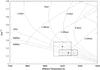 |
Fig. 3 The new position of WASP-3 in the Teff vs. R / M1 / 3 plane. The larger of the two boxes shows the data from the discovery paper. The smaller box shows the error range from this study. The lines show evolutionary tracks from Girardi et al. (2000) for 1.2, 1.3 and 1.4 solar masses and isochrones at 0.1, 0.5, 1, 1.5, 2, 2.5 and 3 billion years. The tracks and isochrones here are for stars with solar metalicity, [ M / H ] = 0. |
Results of MCMC analysis compared to those presented in the literatures.
2.4. Photometric and spectroscopic datasets
In total we used 8 photometric and 2 radial velocity datasets in the MCMC analysis. In addition to the photometric datasets analysed in the discovery paper we included 2 additional sets of photometry taken with the RISE instrument on the 2 m Liverpool Telescope at Observatorio del Roque de Los Muchachos, La Palma (Gibson et al. 2008). The radial velocity data comprised the 26 observations described earlier to target the RM effect, and the 6 out-of-transit observations taken in July and August 2007 also using the SOPHIE spectrograph as described by Pollacco et al. (2008). Figure 3 shows phase-folded plots of the photometric data and the out-of-transit radial velocity measurements.
Values for projected stellar rotation rate, spin-orbit misalignment angle and width of the intrinsic stellar line profile compared to those from the two previous Rossiter-McLaughlin studies of WASP-3b.
3. Results
The resulting values for the system parameters can been seen in Table 1 alongside those taken from the discovery paper, both with their 1σ errors. With the exception of the impact parameter, all values are in agreement within their 1σ uncertainty ranges. Through examination of its relation with the stellar surface gravity Pollacco et al. (2008) suggest that the impact parameter should lie between 0.4 and 0.6 which is in good agreement with the value found in this study of  . Using our method the impact parameter can be more closely constrained, as the properties of the streak of “missing light” also give us a measure of the latitudes of ingress and egress.
One major success of this study is that sensible values in agreement with previous work are produced without having to fix any of the system parameters in place. Pollacco et al. (2008) showed that in order to reconcile the MCMC analysis with spectroscopic diagnostics log g∗ must be between 4.25 and 4.35. Recently Enoch et al. (2010) attempted to reproduce the results from the WASP-3 discovery paper incorporating the Torres mass calibration into the MCMC analysis and found they also needed to fix log g∗ to the value determined by spectroscopic analysis. In this study we left log g∗ as a floating variable and found its value to be  which lies within the range suggested in the discovery paper.
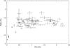 |
Fig. 4 Mass vs. Radius plot for known transiting planets. The two black dots indicate the previous position of WASP-3b from the results in the discovery paper and its updated position from the mass and radius values determined in this study. |
The results produced for the RM parameters are presented in Table 2 along with their one sigma errors. The value we obtained for the projected stellar rotation rate vsini = 13.9 ± 0.03 km s-1 is in good agreement with the value of vsini = 13.4 ± 1.5 km s-1 derived by the analysis of the SOPHIE spectroscopy as presented in the WASP-3 discovery paper (Pollacco et al. 2008). However, our result shows a much greater level of precision. This is because uncertainties on previous estimates of vsini are removed by the fact that we can measure the FWHM of the intrinsic profile directly. Our analysis finds the projected spin-orbit misalignment angle to be  °, which is almost indistinguishable from zero.
Simpson et al. (2010) recently performed a Rossiter-McLaughlin effect analysis of the WASP-3 system with the same data used in this study. They used the method of Hirano et al. (2010) to account for the aforementioned systematic error encountered when trying to calculate vsini by applying the Ohta et al. (2005) method. Their value for vsini of  km s-1 is similar to our value but still slightly larger. For λ they derived a value of
  ° which agrees with our result. In addition to this Tripathi et al. (2010) performed an analysis of a separate set of data and retrieved values that are in good agreement with those found in this study, as can be seen in Table 2.
Using our new, more accurate values for the system parameters we were able to plot the position of WASP-3 on the R / M1 / 3 vs. Teff plane (see Fig. 3). From the MCMC analysis we obtained a value for the stellar effective temperature of Teff = 6332 ± 105 K. Comparing this temperature range with the evolutionary tracks from Girardi et al. (2000) we can get a separate mass estimate for the star of M∗ = 1.23 ± 0.04 M⊙. This is in good agreement with our previous value of  . From the maximum error range we can put an upper limit on the stellar age of around 2 Gyr. This is an improvement on the value presented in Pollacco et al. (2008) which suggested an upper limit of 3.5 Gyr. We cannot put a lower limit on the age of the star using Fig. 3 as the lower range of the errors lie on or beyond the Zero Age Main Sequence. The evolutionary traks of Siess et al. (2000) suggest a pre-main sequence lifetime of 0.13 Gyr for a 1.2 M⊙ star. WASP-3 is a main sequence star, so we can impose this value as an extreme lower age limit. In the discovery paper a lower age estimate of 0.7 Gyr is presented. We can also determine an age estimate from gyrochronology. If we assume that the spin axis of WASP-3 is nearly perpendicular to the line of sight, then vsini = 13.9 km s-1 and Rs = 1.21 R⊙ yields a spin period of 4.5sini days. The period will be shorter than 4.5 days if the inclination is substantially less than 90 degrees.
WASP-3 has 2MASS colour J − K = 0.242. The fastest rotators at the same colour in the 590-Myr-old Coma Berenices open cluster have periods of order 6 days (Collier Cameron et al. 2009). Hyades stars of similar colour also have periods in the range 5 − 6 days at age 625 Myr (Radick et al. 1987), as is also found to be the case in the Praesepe cluster (age 580 Myr) by Delorme et al. (2010, MNRAS, submitted).
If we assume that WASP-3 is spinning down because of angular momentum loss in a hot, magnetically-channeled stellar wind, its spin period should increase with time as the square root of its age. From their calibration of the period-colour relation in Hyades and Praesepe, Delorme et al. (2010) find  yielding a gyrochronological age of 300 Myr for WASP-3, with an uncertainty of order 10 percent. We caution, however, that this relation is only applicable once the spin rate has converged to the asymptotic period-colour relation. While convergence is probably complete for most stars of this mass by the age of 300 Myr, there remains a small possibility that the star could have been born as a relatively slow rotator, leading to over-estimation of the gyrochronological age. We can, however, state with confidence that the gyrochronological age of WASP-3 is substantially less than that of the Hyades.
4. Conclusions
The Rossiter-McLaughlin effect present in the WASP-3 system was analysed from observations made using the SOPHIE spectrograph on the 1.93 m telescope at the Observatoire de Haute-Provence (Simpson et al. 2010). We analysed the observations using a new method developed by Collier Cameron et al. (2010a) which involves decomposing the CCF into its various components and directly tracking the trajectory of the missing starlight across the line profile. This method was incorporated into an MCMC analysis of all photometric and spectroscopic data available for the WASP-3 system and was found to produce good results for the system parameters, helping further constrain the values of the spin-orbit misalignment angle, projected stellar rotation rate and the impact parameter. The value we obtained for the projected spin-orbit misalignment angle  ° is close to zero and agrees with the previous results found by Simpson et al. (2010) and Tripathi et al. (2010). Our value of vsini = 13.9 ± 0.03 km s-1 is in agreement with the value obtained from the spectroscopic broadening but determined to a much higher level of precision. We conclude that this new method of analysing the Rossiter-McLaughlin effect successfully retrieves a more accurate and precise value for the projected stellar spin rate compared with previous measurements, and in doing so it is not vulnerable to the systematic error present in previous methods that require fitting of Gaussians to non-Gaussian CCFs in order to calculate the velocity shifts. It also finds a value for the spin-orbit misalignment angle that agrees with all previous measurements and is of a similar precision. The fact that we clearly detect the signature of the missing light after subtracting the model out-of-transit profile shows that the method works well for a stellar rotation rate that is not much greater than the intrinsic line width. In fact, Collier Cameron et al. (2010a) showed that this method can be successful when vsini is as low as half the value of the intrinsic stellar line width.
The value we obtained for the spin-orbit alignment angle is small enough to support the theory of migration through tidal interaction with a protoplanetary disc. However, recent discoveries of highly misaligned systems (Anderson et al. 2010; Narita et al. 2009) suggest that migration cannot be explained in all cases purely by tidal interactions in a protoplanetary disc. Hebrard et al. (2010) showed that planets with measured spin-orbit angles could be sorted into three distinct populations: firstly, the majority of hot jupiters that are aligned; secondly, the few that are strongly misaligned; and thirdly, the massive planets that are mostly moderately but significantly misaligned. They propose that this could be the signature of three distinct evolution scenarios. Measuring the distribution of alignment angles in Hot Jupiter systems and will help inform theories of planetary migration.
Many transit candidates are rejected from RV follow-up observations if they are found to be rotating too fast for high-precision determination of the RV shift. This is especially true for stars of spectral type earlier than F˜5 which tend to be line-poor rapid rotators. It has already been shown (Collier Cameron et al. 2010b) that using this new method we can successfully confirm the existence of a planet-sized object by measuring the size of the “bump” on the stellar line profile, opening up a way for establishing the existence of close-orbiting planets around rapidly-rotating stars previously inaccessible to planet hunters using the RV method. With this new information we will also be able to investigate any differences in planet formation between solar-type and early-type stars.
For up-to-date exoplanet statistics see http://www.exoplanet.eu
Acknowledgments
The authors of this paper would like to thank the team at the Observatoire de Haute Provence for their support during the observing runs. We also thank the anonymous referee for their helpful and constructive comments. This work is supported by the UK Science and Technology Facilities Council and made use of the ADS database and VizieR catalogue. G. R. M. Miller would like to acknowledge the support and advice given by colleagues during the writing of his first paper.
References
- Anderson, D. R., Hellier, C., Gillon, M., et al. 2010, ApJ, 709, 159 [NASA ADS] [CrossRef] [Google Scholar]
- Borucki, W. J., & for the Kepler Team 2010, ApJ, submitted [arXiv:1006.2799] [Google Scholar]
- Bouchy, F., Hébrard, G., Udry, S., et al. 2009, A&A, 505, 853 [NASA ADS] [CrossRef] [EDP Sciences] [Google Scholar]
- Chatterjee, S., Ford, E. B., Matsumura, S., & Rasio, F. A. 2008, ApJ, 686, 580 [NASA ADS] [CrossRef] [Google Scholar]
- Claret, A. 2004, VizieR Online Data Catalog, 342, 81001 [NASA ADS] [Google Scholar]
- Collier Cameron, A., Wilson, D. M., West, R. G., et al. 2007, MNRAS, 380, 1230 [NASA ADS] [CrossRef] [Google Scholar]
- Collier Cameron, A., Davidson, V. A., Hebb, L., et al. 2009, MNRAS, 400, 451 [NASA ADS] [CrossRef] [Google Scholar]
- Collier Cameron, A., Bruce, V. A., Miller, G. R. M., Triaud, A. H. M. J., & Queloz, D. 2010a, MNRAS, 403, 151 [NASA ADS] [CrossRef] [Google Scholar]
- Collier Cameron, A., Guenther, E., Smalley, B., et al. 2010b, MNRAS, 407, 507 [NASA ADS] [CrossRef] [Google Scholar]
- Enoch, B., Collier Cameron, A., Parley, N. R., & Hebb, L. 2010, A&A, 516, A33 [NASA ADS] [CrossRef] [EDP Sciences] [Google Scholar]
- Fabrycky, D., & Tremaine, S. 2007, ApJ, 669, 1298 [NASA ADS] [CrossRef] [Google Scholar]
- Gaudi, B. S., & Winn, J. N. 2007, ApJ, 655, 550 [NASA ADS] [CrossRef] [Google Scholar]
- Gibson, N. P., Pollacco, D., Simpson, E. K., et al. 2008, A&A, 492, 603 [NASA ADS] [CrossRef] [EDP Sciences] [Google Scholar]
- Giménez, A. 2006, ApJ, 650, 408 [NASA ADS] [CrossRef] [Google Scholar]
- Girardi, L., Bressan, A., Bertelli, G., & Chiosi, C. 2000, A&AS, 141, 371 [Google Scholar]
- Goldreich, P., & Tremaine, S. 1980, ApJ, 241, 425 [NASA ADS] [CrossRef] [MathSciNet] [Google Scholar]
- Hebrard, G., Desert, J., Diaz, R. F., et al. 2010, A&A, 516, A95 [NASA ADS] [CrossRef] [EDP Sciences] [Google Scholar]
- Hirano, T., Suto, Y., Taruya, A., et al. 2010, ApJ, 709, 458 [NASA ADS] [CrossRef] [Google Scholar]
- Jurić, M., & Tremaine, S. 2008, ApJ, 686, 603 [NASA ADS] [CrossRef] [Google Scholar]
- Kozai, Y. 1962, AJ, 67, 591 [Google Scholar]
- Lin, D. N. C., Bodenheimer, P., & Richardson, D. C. 1996, Nature, 380, 606 [NASA ADS] [CrossRef] [Google Scholar]
- Mayor, M., & Queloz, D. 1995, Nature, 378, 355 [NASA ADS] [CrossRef] [Google Scholar]
- McLaughlin, D. B. 1924, Pop. Astron., 32, 558 [NASA ADS] [Google Scholar]
- Nagasawa, M., Ida, S., & Bessho, T. 2008, ApJ, 678, 498 [NASA ADS] [CrossRef] [Google Scholar]
- Narita, N., Sato, B., Hirano, T., & Tamura, M. 2009, PASJ, 61, L35 [NASA ADS] [Google Scholar]
- Nelson, R. P., Papaloizou, J. C. B., Masset, F., & Kley, W. 2000, MNRAS, 318, 18 [NASA ADS] [CrossRef] [Google Scholar]
- Ohta, Y., Taruya, A., & Suto, Y. 2005, ApJ, 622, 1118 [NASA ADS] [CrossRef] [Google Scholar]
- Pollacco, D., Skillen, I., Collier Cameron, A., et al. 2008, MNRAS, 385, 1576 [NASA ADS] [CrossRef] [Google Scholar]
- Radick, R. R., Thompson, D. T., Lockwood, G. W., Duncan, D. K., & Baggett, W. E. 1987, ApJ, 321, 459 [NASA ADS] [CrossRef] [Google Scholar]
- Rossiter, R. A. 1924, ApJ, 60, 15 [NASA ADS] [CrossRef] [Google Scholar]
- Sasselov, D. D., & Lecar, M. 2000, ApJ, 528, 995 [NASA ADS] [CrossRef] [Google Scholar]
- Siess, L., Dufour, E., & Forestini, M. 2000, A&A, 358, 593 [NASA ADS] [Google Scholar]
- Simpson, E. K., Pollacco, D., Hébrard, G., et al. 2010, MNRAS, 405, 1867 [NASA ADS] [Google Scholar]
- Torres, G., Andersen, J., & Giménez, A. 2010, A&ARv, 18, 67 [Google Scholar]
- Triaud, A. H. M. J., Queloz, D., Bouchy, F., et al. 2009, A&A, 506, 377 [NASA ADS] [CrossRef] [EDP Sciences] [Google Scholar]
- Tripathi, A., Winn, J. N., Johnson, J. A., et al. 2010, ApJ, 715, 421 [NASA ADS] [CrossRef] [Google Scholar]
- Weidenschilling, S. J., & Marzari, F. 1996, Nature, 384, 619 [NASA ADS] [CrossRef] [PubMed] [Google Scholar]
- Winn, J. N., Noyes, R. W., Holman, M. J., et al. 2005, ApJ, 631, 1215 [NASA ADS] [CrossRef] [Google Scholar]
- Winn, J. N., Johnson, J. A., Marcy, G. W., et al. 2006, ApJ, 653, L69 [NASA ADS] [CrossRef] [Google Scholar]
- Winn, J. N., Johnson, J. A., Peek, K. M. G., et al. 2007, ApJ, 665, L167 [NASA ADS] [CrossRef] [Google Scholar]
- Wu, Y., & Murray, N. 2003, ApJ, 589, 605 [NASA ADS] [CrossRef] [EDP Sciences] [Google Scholar]
All Tables
Values for projected stellar rotation rate, spin-orbit misalignment angle and width of the intrinsic stellar line profile compared to those from the two previous Rossiter-McLaughlin studies of WASP-3b.
All Figures
|
Fig. 1 Upper panel: phase-folded plot of the 6 out-of-transit radial velocity measurements which are not affected by any time-varying asymmetry of the line-profile. The out-of-transit RV fit was calculated using the velocity semi-amplitude, orbital eccentricity, arguement of periastron and true anomaly. The position of the planet over the stellar disc, ratio of star/planet radii, impact parameter and non-linear limb darkening coefficients were used to model the RM anomaly during transit. Lower panel: phase-folded plot of all 8 sets of photometric data analysed in this study. |
| In the text | |
|
Fig. 2 Top: residual map of time series CCFs with the model spectrum subtracted leaving the bright time-variable feature due the light blocked by the planet. Bottom: here the best-fit model for the time-variable feature has also been removed to show the overall residual. The horizontal dotted line marks the phase of mid-transit. The shift of this line from zero shows the underlying systemic radial velocity. The two vertical dashed lines are at ± vsini from the stellar radial velocity (marked by the vertical dotted line). The crosses on the vertical dotted line denote the two points of contact at both ingress and egress. |
| In the text | |
|
Fig. 3 The new position of WASP-3 in the Teff vs. R / M1 / 3 plane. The larger of the two boxes shows the data from the discovery paper. The smaller box shows the error range from this study. The lines show evolutionary tracks from Girardi et al. (2000) for 1.2, 1.3 and 1.4 solar masses and isochrones at 0.1, 0.5, 1, 1.5, 2, 2.5 and 3 billion years. The tracks and isochrones here are for stars with solar metalicity, [ M / H ] = 0. |
| In the text | |
|
Fig. 4 Mass vs. Radius plot for known transiting planets. The two black dots indicate the previous position of WASP-3b from the results in the discovery paper and its updated position from the mass and radius values determined in this study. |
| In the text | |
Current usage metrics show cumulative count of Article Views (full-text article views including HTML views, PDF and ePub downloads, according to the available data) and Abstracts Views on Vision4Press platform.
Data correspond to usage on the plateform after 2015. The current usage metrics is available 48-96 hours after online publication and is updated daily on week days.
Initial download of the metrics may take a while.