| Issue |
A&A
Volume 523, November-December 2010
|
|
|---|---|---|
| Article Number | A54 | |
| Number of page(s) | 8 | |
| Section | Stellar structure and evolution | |
| DOI | https://doi.org/10.1051/0004-6361/201014966 | |
| Published online | 16 November 2010 | |
Core properties of α Centauri A using asteroseismology
1
Institut d’Astrophysique et de Géophysique de l’Université de
Liège,
Allée du 6 Août 17,
4000
Liège,
Belgium
e-mail: This email address is being protected from spambots. You need JavaScript enabled to view it.
; This email address is being protected from spambots. You need JavaScript enabled to view it.
; This email address is being protected from spambots. You need JavaScript enabled to view it.
2
Instituut voor Sterrenkunde, Katholieke Universiteit Leuven,
Celestijnenlaan
200D, 3001
Leuven,
Belgium
e-mail: This email address is being protected from spambots. You need JavaScript enabled to view it.
3 Sydney Institute for Astronomy (SIfA), School of Physics A28,
University of Sydney, NSW 2006, Australia
e-mail: This email address is being protected from spambots. You need JavaScript enabled to view it.
4
Danish AsteroSeismology Centre (DASC), Department of Physics and
Astronomy, Aarhus University, 8000
Aarhus C,
Denmark
e-mail: This email address is being protected from spambots. You need JavaScript enabled to view it.
; campante]@phys.au.dk
5
Centro de Astrofísica da Universidade do Porto,
Rua das Estrelas,
4150-762
Porto,
Portugal
6
Observatoire de Genève, Université de Genève,
51 chemin des
Maillettes, 1290
Sauverny,
Switzerland
Received:
10
May
2010
Accepted:
14
July
2010
Abstract
Context. A set of long and nearly continuous observations of α Centauri A should allow us to derive an accurate set of asteroseismic constraints to compare to models, and make inferences on the internal structure of our closest stellar neighbour.
Aims. We intend to improve the knowledge of the interior of α Centauri A by determining the nature of its core.
Methods. We combined the radial velocity time series obtained in May 2001 with three spectrographs in Chile and Australia: CORALIE, UVES, and UCLES. The resulting combined time series has a length of 12.45 days and contains over 10 000 data points and allows to greatly reduce the daily alias peaks in the power spectral window.
Results. We detected 44 frequencies that are in good overall agreement with previous studies, and found that 14 of these show possible rotational splittings. New values for the large (Δν) and small separations (δν02, δν13) have been derived.
Conclusions. A comparison with stellar models indicates that the asteroseismic constraints determined in this study (namely r10 and δν13) allows us to set an upper limit to the amount of convective-core overshooting needed to model stars of mass and metallicity similar to those of α Cen A.
Key words: stars: individual:αCen A / stars: oscillations / stars: variables: general / stars: interiors
© ESO, 2010
1. Introduction
During the last decade, the visual binary stellar system α Centauri turned out to be a very interesting asteroseismic target to observe and model because of its proximity and of the similarity of these stars to the Sun. Moreover, the mass of the primary component is very close to the limit above which stellar models predict the onset of convection in the energy-generating core. This makes the theoretical study of α Cen A particularly valuable for testing the poorly-modelled treatment of convection and extra-mixing in the central regions of low-mass stars.
The proximity of α Cen (d = 1.34 pc) provides a relatively well determined parallax, π = 747.1 ± 1.2 mas (Söderhjelm 1999). This visual binary system shows an eccentric orbit (e = 0.519) with a period of almost 80 years and so the masses of the two components are very well constrained. The more luminous component, α Cen A, is a G2V star with a mass of 1.105 ± 0.007M⊙. The secondary, α Cen B, is a cooler K1V star with a mass of 0.934 ± 0.006M⊙ (Pourbaix et al. 2002), so they bracket the Sun in mass. Their effective temperatures are Teff,A = 5810 ± 50 K and Teff,B = 5260 ± 50 K (see Porto de Mello et al. 2008). Kervella et al. (2003) have measured the angular diameters of α Cen A and B with VINCI/VLTI. Combining with the parallax gave linear radii for the two stars: RA = 1.224 ± 0.003 R⊙ and RB = 0.863 ± 0.005 R⊙. Masses and radii allow determination of the surface gravities: log gA = 4.307 ± 0.005 and log gB = 4.538 ± 0.008, an accuracy rarely reached in stars other than the Sun. Moreover, thees brightness of both components of the system (VA = −0.01 and VB = 1.33) allows the acquisition of extremely high-quality spectra.
Asteroseismic data have been obtained by several teams. The first unambiguous detection of
p-modes in α Cen A was made by Bouchy
& Carrier (2001, 2002) during a
13-night campaign with the spectrograph CORALIE, confirming the earlier claimed detection
made by Schou & Buzasi (2000) with the WIRE
satellite. Bouchy & Carrier (2002) detected 28
modes with angular degrees ℓ = 0,1 and 2. At the same
time, another team (Butler et al. 2004; Bedding et al. 2004) made observations during five nights
from Chile with UVES and from Australia with UCLES, and detected 42 frequencies with
ℓ = 0,1,2 and 3. Kjeldsen et al. (2005) also provided a value of the mode lifetime for
α Cen A of  days. Fletcher et al. (2006) then carried out a re − analysis
of the WIRE observations, resulting in additional asteroseismic data. In particular, they
suggested two values of the rotational frequency, 0.54 ± 0.22μHz and
0.64 ± 0.25μHz, using two different analysis methods, and a mode lifetime
of 3.9 ± 1.4 days. More recently, Bazot et al. (2007)
detected 34 modes with the HARPS spectrograph in Chile, and suggested five rotational
splittings for ℓ = 2 modes. Asteroseismic data have also been obtained for
the B component (Carrier & Bourban 2003;
Kjeldsen et al. 2005).
days. Fletcher et al. (2006) then carried out a re − analysis
of the WIRE observations, resulting in additional asteroseismic data. In particular, they
suggested two values of the rotational frequency, 0.54 ± 0.22μHz and
0.64 ± 0.25μHz, using two different analysis methods, and a mode lifetime
of 3.9 ± 1.4 days. More recently, Bazot et al. (2007)
detected 34 modes with the HARPS spectrograph in Chile, and suggested five rotational
splittings for ℓ = 2 modes. Asteroseismic data have also been obtained for
the B component (Carrier & Bourban 2003;
Kjeldsen et al. 2005).
Table of the main features of the three campaigns.
Table of the level noise (in the power spectrum) for the different campaigns and their combination.
The α Cen system has been also extensively modelled. Guenther & Demarque (2000), Morel et al. (2000) and Noels et al. (1991) performed a calibration based only on non-asteroseismic constraints. They found that two kinds of models, one with a radiative core and the other with a convective one, could satisfy these constraints. Subsequently, the high-quality non-asteroseismic constraints together with asteroseismic constraints stimulated new calibrations of the stellar system (Thévenin et al. 2002; Thoul et al. 2003; Eggenberger et al. 2004; Miglio & Montalbán 2005). Although these authors succeeded to fit some of the asteroseismic constraints, they were not in a position to draw a definite conclusion on the convective versus radiative nature of the core of α Centauri A. To perform such a discrimination, all teams suggested that more accurate asteroseismic constraints were needed.
In the present paper, the May 2001 data of Bouchy & Carrier (2002) from CORALIE and of Bedding et al. (2004) from UVES and UCLES have been unified to compute a combined velocity time series in order to reduce the effect of daily aliases in the power spectrum. The objective is to provide a more accurate set of asteroseismic constraints that allows a better comparison with theoretical models and a clear discrimination between them.
Section 2 describes the different data sets and their main features, along with the method used to analyse the acoustic spectrum. Section 3 presents the frequencies and amplitudes detected, along with new values for the large and small separations and a rotational frequency. In the Sect. 4, we compare these new observational constraints with the models of α Cen A presented by Miglio & Montalbán (2005). Section 5 is dedicated to the conclusions.
2. Data and methods
2.1. Data sets
α Cen A was observed in May 2001 in Chile by Bouchy & Carrier (2002) during a 13-night campaign with the CORALIE fiber-fed échelle spectrograph, mounted on the 1.2 m Euler Swiss telescope at the ESO La Silla Observatory (Bouchy & Carrier 2001, 2002). Another team (Butler et al. 2004; Bedding et al. 2004) made two-site observations over five nights from Chile and Australia. They used UVES (UV-Visual Echelle Spectrograph) at the 8.2 m Unit Telescope 2 (Kueyen) of the VLT (Very Large Telescope) in Chile, and UCLES (University College London Echelle Spectrograph) at the 3.9 m AAT (Anglo-Australian Telescope) at Siding Spring Observatory in Australia. These two spectrographs were provided a stable wavelength reference using an iodine cell (see Butler et al. 1996).
The median cadence of the data set was one spectrum every 150 s for CORALIE, 26 s for UVES and 20 s for UCLES. The durations of the observations and the total number of spectra are given in Table 1.
Figure 1 shows the times series of the different spectrographs. One can see in Tables 1 and 2 that each time series has its own advantages. CORALIE has the longest time series, and thus the best frequency resolution (0.93μHz). UVES data have the best signal-to-noise ratio in the power spectrum (see Table 2). One can also note (Fig. 1) that the UCLES nights, observed from Australia, fill some gaps in the CORALIE and UVES nights, observed from Chile. This is important when combining the data, as discussed below.
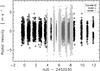 |
Fig. 1 Combined time series of CORALIE, UVES and UCLES. One can see that the UCLES data, which were taken in Australia, fill several gaps in the time series of the CORALIE and UVES data, taken in Chile. This will allow a better detection of p-modes frequencies by reducing the daily aliases in the spectrum of the star (see text for details). |
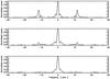 |
Fig. 2 Comparison of the spectral windows of the time series of the CORALIE data (top panel) and the one of the combined time series of the CORALIE, UVES and UCLES data with standard weights (middle panel) and sidelobe-optimised weights (bottom panel). The daily aliases are already much reduced in the case of the combined time series with standard weights, as expected from the fact that UCLES nights fill several gaps in the CORALIE and UVES time series. |
2.2. Combining data sets and weighting
Combing the different velocity time series allows us to reduce the aliases at 1 d-1 (or 11.57 μHz) that arise from the daily gaps in the time series. The top panel of Fig. 2 shows the spectral window of the CORALIE data alone and the middle panel shows the result for the combined time series, using standard weights (see below). The 1 d-1 alias peaks have been reduced by a factor ~2.6 in power between the two.
We used the Lomb-Scargle modified algorithm, suited for unevenly spaced data (Lomb 1976; Scargle 1982), to compute the power spectrum of the combined velocity time series. We used three different weighting schemes, which we will refer to as standard weights, sidelobe-optimised weights and noise-optimised weights:
-
1.
We used the measurement uncertainties, σi, as weights in calculating the power spectrum, which is displayed in Fig. 3. With these so-called standard weights
 , the mean white noise
level in the power spectrum, computed between 7.5 and 15 mHz, is
8.58 × 10⁻⁴ m2 s-2. Assuming the noise to be
white (
, the mean white noise
level in the power spectrum, computed between 7.5 and 15 mHz, is
8.58 × 10⁻⁴ m2 s-2. Assuming the noise to be
white ( ),
the mean noise level in the amplitude spectrum is 2.59 cm s-1.
),
the mean noise level in the amplitude spectrum is 2.59 cm s-1. -
2.
We applied the method described by Bedding et al. (2004) in which weights are optimised in order to reduce the daily aliases. We adjusted the weights on a night-by-night basis in order to optimise the window function. To be specific, we allocated separate adjustment factors to each of the CORALIE, UVES and UCLES nights. The weights on each night were multiplied by these factors and the spectral window was calculated, and this process was iterated to minimize the height of the sidelobes. The spectral window of the sidelobe-optimised spectrum is displayed in Fig. 2 (bottom panel).
-
3.
The third power spectrum was computed by means of noise-optimised weights, as described by Arentoft et al. (2008). The short-term variations in the uncertainty time series were first removed by bandpass-filtering. This removed fluctuations in the weights on the timescale of the stellar oscillations. We also studied the velocity residuals in which both the slow variations and the stellar oscillations were removed. We compared the velocity residuals, ri with the corresponding uncertainty estimates, σi. Bad data points are those for which the ratio | ri/σi | is large, i.e., where the residual velocity deviates from zero by more than expected from the uncertainty estimate. Bad data points were then down-weighted by dividing all σi by
 ,
where f(xi) is an
analytical function:
,
where f(xi) is an
analytical function: 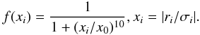 (1)The adjustable
parameter x0 controls the amount of down weighting; it
sets the values of
|ri/σi|
for which the weights are multiplied by 0.5, and so it determines how bad a data
point should be before it is down weighted. The optimum choice for
x0 was found through iteration. For each trial value
of x0, the noise level was determined from a time series
in which all power had been removed at both the low-frequency noise and the
high-frequency oscillations. We chose the x0 that
resulted in the lowest noise in the power spectrum. These weights allowed us to
diminish the level of noise (see Table 2).
(1)The adjustable
parameter x0 controls the amount of down weighting; it
sets the values of
|ri/σi|
for which the weights are multiplied by 0.5, and so it determines how bad a data
point should be before it is down weighted. The optimum choice for
x0 was found through iteration. For each trial value
of x0, the noise level was determined from a time series
in which all power had been removed at both the low-frequency noise and the
high-frequency oscillations. We chose the x0 that
resulted in the lowest noise in the power spectrum. These weights allowed us to
diminish the level of noise (see Table 2).
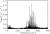 |
Fig. 3 Power spectrum of the combined time series of CORALIE, UVES and UCLES (standard weights). |
Table of the frequencies detected (in μHz).
2.3. Frequency analysis
The method used to extract the modes was the standard pre-whitening procedure. It consists of locating the highest peak in the region that contains the oscillation frequencies and subtracting the corresponding sinusoid from the time series. We then computed a new power spectrum, located the highest peak and iterated the procedure until no peaks remained above S/N = 3.
When a peak in the power spectrum is removed by subtracting the corresponding sinusoid from the time series, the daily aliases associated with this peak also disappear from the power spectrum. This works well for high-amplitude peaks but at low amplitudes the reinforcement by noise may cause an alias peak to be mistaken for the real peak. By analysing three versions of the power spectrum, we hoped to reduce this problem. It should also be kept in mind that if the oscillation modes are resolved, i.e., the oscillations have a shorter lifetime than the duration of the observations, then each oscillation mode will produce multiple peaks.
The uncertainties on the frequencies were computed using the formula of Libbrecht (1992): 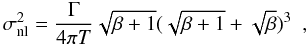 (2)where
T is the total length of the time series, β is the
reciprocal of the signal-to-noise ratio of the mode, and Γ is the line-width of the mode.
Note that Γ is related to the mode lifetime (τ) via
Γ = 1/πτ. In fact, the modes are not resolved in the
spectrum and so we set Γ to the frequency resolution, 0.93μHz, which is
the same value that would be deduced from the lifetime of 3.9 ± 1.4 d reported by Fletcher et al. (2006).
(2)where
T is the total length of the time series, β is the
reciprocal of the signal-to-noise ratio of the mode, and Γ is the line-width of the mode.
Note that Γ is related to the mode lifetime (τ) via
Γ = 1/πτ. In fact, the modes are not resolved in the
spectrum and so we set Γ to the frequency resolution, 0.93μHz, which is
the same value that would be deduced from the lifetime of 3.9 ± 1.4 d reported by Fletcher et al. (2006).
3. Results
3.1. Mode identification and échelle diagram
In solar-like stars, p-mode oscillations produce a characteristic comb-like structure in
the power spectrum, which is well-approximated by the asymptotic relation (Tassoul 1980): 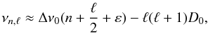 (3)where
Δν0 = ⟨νn,ℓ − νn − 1,ℓ⟩
and D0 ≈
(3)where
Δν0 = ⟨νn,ℓ − νn − 1,ℓ⟩
and D0 ≈  .
The two quantum numbers n and ℓ correspond to the radial
order and angular degree, respectively. Since the stellar disk is not resolved, only the
lowest degree modes (ℓ ≤ 3) can be detected. In case of stellar rotation,
a third quantum number, m, describes the splitting of the frequencies:
.
The two quantum numbers n and ℓ correspond to the radial
order and angular degree, respectively. Since the stellar disk is not resolved, only the
lowest degree modes (ℓ ≤ 3) can be detected. In case of stellar rotation,
a third quantum number, m, describes the splitting of the frequencies:
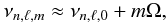 (4)with
− ℓ ≤ m ≤ ℓ and with Ω being the
frequency of the rotation.
(4)with
− ℓ ≤ m ≤ ℓ and with Ω being the
frequency of the rotation.
In the power spectrum of α Cen A, displayed in Fig. 3 (computed with the standard weights), we see a series of peaks between 1.8 mHz and 3 mHz, as expected for solar-like oscillations in a star of this mass and radius. A periodicity of about 106μHz is clear in the power spectrum, a fact that can also be seen in its autocorrelation. In order to identify the angular degree ℓ of each mode, the power spectrum has been cut in slices of 106μHz and summed, in order to build the collapsed échelle diagram (Fig. 5). This diagram shows peaks corresponding to ℓ = 0,1,2 and 3 modes. We also see in this figure that the side-lobes due to aliases, which often complicate the analysis, are significantly reduced. This collapsed échelle diagram allows us to identify clearly the modes ℓ = 0,1,2 and the possible presence of ℓ = 3 modes, and to reject other frequencies that were obviously false p-modes extractions. Our identification agrees with those previously published.
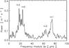 |
Fig. 5 Collapsed échelle diagram. The first major peak, below 20μHz is an ℓ = 2 and the second, at 25μHz is an ℓ = 0. The two peaks around 65μHz belongs to the ℓ = 3 mode and the last peak, at 75μHz is an ℓ = 1. |
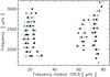 |
Fig. 6 Echelle diagram of the new frequencies (black asterisks) and those reported by earlier studies: CORALIE (Bouchy & Carrier 2002) (blue squares), UVES-UCLES (Bedding et al. 2004) (red triangles), HARPS (Bazot et al. 2007) (green diamonds). |
Table 3 and Fig. 4 give the 44 modes that have been detected. For the particular case of the ℓ = 3 modes, we paid attention to the proximity of these modes to the daily alias peaks of the ℓ = 1 modes. The sidelobe-optimised power spectrum, where the aliases were further diminished by optimising the weights, helped us to ensure that the peaks detected were ℓ = 3 modes and not aliases of ℓ = 1 modes.
The échelle diagram displayed in Fig. 6 is a convenient tool to illustrate the properties of a solar-like star. It was introduced by Grec et al. (1983) to identify the degree ℓ of solar modes. It is computed by plotting the detected frequencies modulo the large separation Δν. In Fig. 6, we present a comparison of the frequencies detected in this work with those detected in previous studies. This is generally satisfactory agreement. Some of our frequencies are multiple, as indicated in Table 3, which could be attributed to the stellar rotation or to the modes being resolved.
3.2. Large and small separations
The left panel of Fig. 7 shows the large separation as a function of frequency for the modes of degree ℓ = 0. To compute the average large separation, Δν0, we fitted a linear relation νn,ℓ = n(Δν0 + ϵ), where ϵ is a constant and the slope gives the mean large separation. We also did this for each value of ℓ and made a weighted sum to obtain 105.9 ± 0.3μHz. This is in good agreement with previously published values of 106.1 ± 0.4μHz (Bedding et al. 2004) and 105.9 ± 0.3μHz (Bazot et al. 2007).
For the small separation, δν02, we computed a mean of the values shown in the right panel of the figure, and found 5.8 ± 0.1μHz (the error bar is underestimated because it does not take into account the additional error due to splittings). Our value is slightly lower than previously published values of 7.1 ± 0.6μHz (Bedding et al. 2004) and 6.9 ± 0.4μHz (Bazot et al. 2007). Note, however, that our study spans a different and wider region in frequency than that by Bazot et al. (2007), and our combined time series has higher resolution than the UVES/UCLES data alone. Our result is, however, in good agreement with Bouchy & Carrier (2002).
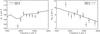 |
Fig. 7 Left panel: comparison of the large separation for ℓ = 0 modes with the one derived by Miglio & Montalbán (2005) in their models A3, with radiative core and A4, with convective core. Right panel: comparison of the small separation with the models A3 and A4. The agreement between the data points of our study and the models is significantly better than for the small separation obtained by Bouchy & Carrier (2002) (see Miglio & Montalbán 2005) |
Table of the amplitudes fitted by least squares fit (in cm s-1) and their S/N ratios associated.
3.3. Rotational splittings and frequency
Fletcher et al. (2006) reanalysed the WIRE data obtained by Schou & Buzasi (2000). Fitting to the autocovariance function (ACF), they obtained a value of 0.54 ± 0.22μHz for the rotational splitting. They also performed a fit to the power spectrum and obtained 0.64 ± 0.25μHz, but suggested that this value is less robust. Bazot et al. (2007) (based on the data of Pourbaix et al. 2002 and Saar & Osten 1997) found Ω = 0.51 ± 0.13μHz. However from the 5 splittings of ℓ = 2 modes observed by Bazot et al. (2007), one can derive a rotational frequency of 0.75 ± 0.22μHz, significantly higher than the other values.
The visibilities of the multiplet components depend on the inclination angle i of the rotation axis of the star (e.g. Gizon & Solanki 2003; Ballot et al. 2006, 2008). We recall that a high value of the inclination angle leads to the peaks with m = ± ℓ being higher than the others in the multiplet. Bouchy & Carrier 2002 adopted an inclination of i = 79° (Pourbaix et al. 2002) to estimate the visibilities of the split modes. They assumed that the inclination of the star and of the orbit are the same, which is not necessarily the case. Their results for the visibilities are given in Table 5, from which we see that the two most visible peaks of a split ℓ = 1 mode are those with m = ±1. Thus, if we take a value of 0.5 μHz for the rotation frequency, these peaks are expected to be separated by 1 μHz, and will have equal amplitudes. For an ℓ = 2 mode, the distance between the two major peaks is 2 μHz and the quantum numbers are m = ±2, while for an ℓ = 3 mode, the distance is 3 μHz and m = ±3. That is what we would expect to find for such a rotation frequency.
We have detected 14 possible splittings, listed in Table 3. They are shown in Fig. 8, normalized
according to their most probable m quantum number. However, note that one
should be cautious with the ℓ = 1 splittings. Firstly, they could be
caused by the finite mode lifetime (3.9 ± 1.4 days according to Fletcher et al. 2006 and days according
to Kjeldsen et al. 2005). Secondly, amplitude
ratios between prograde (m = +1) and retrograde
(m = −1) modes are found to be approximately a factor two, which is not
consistent with expected mode visibility ratios. For the modes of higher angular degree,
the frequency separation between m = + ℓ and
m = − ℓ mode is higher than the mode line-width
inferred by both Kjeldsen et al. (2005) and Fletcher et al. (2006). In addition, mode amplitude
ratios are compatible with mode visibility ratios (see Table 4 and 5), except for the
2358.3/2359.6 mode, which is therefore not a good candidate of splitting.
We computed a rotational frequency of 0.77 ± 0.05μHz by taking the weighted mean of all splittings. If we exclude the ℓ = 1 splittings, which have values close to the limit of resolution, a value of 0.75 ± 0.05μHz is found. This last value will be kept as more secure for the reasons mentioned above. The rotation frequency we have found, although greater, is within one sigma of both values derived by Fletcher et al. (2006). The value given by Bazot et al. (2007), Ω = 0.51 ± 0.13μHz, is only based on spectroscopic data (Pourbaix et al. 2002; Saar & Osten 1997). From their identified ℓ = 2, we can derive a splitting of 0.75 ± 0.22μHz, in good agreement with our value. One has to keep in mind that our value, 0.75 ± 0.05μHz, is based on measurements of the rotational frequency by means of an identification of split modes. Note that this value indicates a significantly faster rotation rate than the one determined by Jay et al. (1997) and Saar & Osten (1997), who found a period between 20 and 30 days. Our rotational frequency, if correct, corresponds to a period of about 15 days.
Table of the expected amplitudes ratios of split modes, in function of ℓ and m quantum numbers, compared to the amplitude of the non-split mode (ℓ = 0, m = 0).
4. Comparison with models
A great number of theoretical studies dealing with α Cen A have been published in the recent years, in particular since solar-like oscillations were first detected by Bouchy & Carrier (2002) (see e.g. Thévenin et al. 2002; Thoul et al. 2003; Eggenberger et al. 2004; Miglio & Montalbán 2005; Yildiz 2007). The A component of the binary system is indeed particularly interesting to model because its mass, 1.105 ± 0.007M⊙ (Pourbaix et al. 2002), is close to the limit above which stars in the main sequence phase (MS) keep the convective core they developed on the pre-MS (PMS).
Miglio & Montalbán (2005) performed several calibrations of the α Centauri system to fit both classical constraints (photometric, spectroscopic and astrometric) as well as the asteroseismic constraints given by Bouchy & Carrier (2002) and Carrier & Bourban (2003). They found that models with either a radiative or a convective core could reproduce equally well classical constraints, as we show in Fig. 9. An overshooting parameter αOV > 0.151 was found to be sufficient in the calibrations for a convective core to persist after the PMS. We see in Fig. 9 that the effect of overshooting is clearly important in the evolution of the star: the evolutionary track of model A4 (computed with αOV = 0.2) has a similar behaviour to that of more massive stars, where a convective core is present regardless of the amount of overshooting adopted.
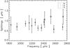 |
Fig. 8 Size of the splittings for ℓ = 1,2 and 3 modes, divided by 2m. The mean of these splittings should give the value of the rotation frequency of the star (see text). |
Despite their similar photospheric constraints, models A3 and A4 have significantly
different interiors. While model A3 has a radiative energy-generating core characterized by
a smooth chemical composition gradient, model A4 presents an adiabatically stratified
fully-mixed region extending to about 10% the total mass of the star, and a sharp chemical
composition gradient at its edge. This different structure, as shown by Miglio & Montalbán (2005), leaves a clear
signature in the oscillation frequencies, in particular in the asteroseismic quantities
r10 and r02 (Roxburgh & Vorontsov 2003):
 (5)with the small separation
between ℓ = 1 and ℓ = 0 modes defined as:
(5)with the small separation
between ℓ = 1 and ℓ = 0 modes defined as:
 (6)Note we have adopted the
5-point definition for δν10 proposed by Roxburgh & Vorontsov (2003), which is smoother
than the conventional 3-point separation. These ratios are known to be largely independent
of outer layers of the star, and provide a reliable probe of the near-core structure.
However, the uncertainties on the oscillation frequencies prevented Miglio & Montalbán (2005) from drawing firm conclusions on the
core properties of α Cen A. The sensitivity of
δν10 to the properties of the core has also
been discussed by Deheuvels et al. (2010).
(6)Note we have adopted the
5-point definition for δν10 proposed by Roxburgh & Vorontsov (2003), which is smoother
than the conventional 3-point separation. These ratios are known to be largely independent
of outer layers of the star, and provide a reliable probe of the near-core structure.
However, the uncertainties on the oscillation frequencies prevented Miglio & Montalbán (2005) from drawing firm conclusions on the
core properties of α Cen A. The sensitivity of
δν10 to the properties of the core has also
been discussed by Deheuvels et al. (2010).
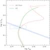 |
Fig. 9 HR diagram showing the evolutionary tracks of model A3 (with a radiative core) and model A4 (with a convective core) from Miglio & Montalbán (2005). The error boxes for Teff, log L/L⊙, and radii correspond to 1σ (solid line) and 2σ (dashed-line). |
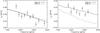 |
Fig. 10 Left: comparison of the r02 constraint with the models A3 and A4. Right: comparison of the r10 constraint with the models A3 and A4. The data points seem clearly to agree with the model A3, a fact that was not established with the data of Bouchy & Carrier (2002). Indeed, all their points for the r10 asteroseismic constraint were situated between the curves of the models A3 and A4 (see Miglio & Montalbán 2005). |
In Figs. 10 and 11 we compare the frequency separations r10, r02 and δν13 derived by our study with those of models A3 and A4. Note that when two peaks were identified for a given mode νn,ℓ, we assumed that they are modes with opposite m-degrees and took the average to get the mode νn,ℓ,0. When only one peak was detected for a given non-radial mode, it was assumed to be m = 0, which leads to possible bias that may explain some of the outliers of Figs. 7, 10 and 11. Although r02 does not discriminate between models with radiative (A3) and with convective (A4) core, r10 clearly favours model A3, a fact that could not be established with the data of Bouchy & Carrier (2002) in the work of Miglio & Montalbán (2005). Moreover, the availability of ℓ = 3 modes in the power spectrum also allows such a discrimination via the small separation δν13: this comparison further supports the conclusion that a model with a convective core having about 10% of the stellar mass, such as model A4, can be rejected on the basis of the asteroseismic constraints.
5. Summary
Observations of α Centauri A allowed us to derive an accurate set of asteroseismic constraints to compare with models and make inferences on the internal structure of our closest stellar neighbour. We combined the time series obtained by three spectrographs during a multi-site observation campaign carried out in 2001. While the combined time series is as long as the one of Bouchy & Carrier (2002), it contains almost 5 times more spectra, and daily aliases are reduced by a factor 2.6. These improvements in the time series allowed us to detect 44 frequencies with ℓ = 0,1,2,3 by means of a pre-whitening algorithm, of which 14 showed possible rotational splittings. Five of these splittings have been obtained for modes ℓ = 3, the first time in α Cen A. A new échelle diagram has been derived and is in overall good agreement with the results of the previous analyses. New values of the large and small separations have been derived from the set of frequencies.
A comparison with the stellar models by Miglio & Montalbán (2005) indicates that the asteroseismic constraints determined in this study (namely r10 and δν13) allow us to set an upper limit on the amount of convective-core overshooting needed to model stars of mass and metallicity similar to those of α Cen A. As described in section 4, a model of the star with a radiative core represents the observed r10 and δν13 separations significantly better than the model with a convective core.
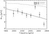 |
Fig. 11 Comparison of the δν13 constraint with the models A3 and A4. The model without overshooting is in a better agreement with the data than the model with overshooting. |
The extension of the overshooting layer in the models is defined as ov = αOVmin(Hp(rc),rc), where Hp is the pressure scale height and rc the radius of the convective core
Acknowledgments
F.C. is a postdoctoral fellow of the Fund for Scientific Research, Flanders (FWO). A.M. is a postdoctoral researcher of the “Fonds
de la recherche scientifique” FNRS, Belgium. This work was also supported financially by the Australian Research Council and the Danish Natural Science Research Council.
References
- Arentoft, T., Kjeldsen, H., Bedding, T. R., et al. 2008, ApJ, 687, 1180 [NASA ADS] [CrossRef] [Google Scholar]
- Ballot, J., García, R. A., & Lambert, P. 2006, MNRAS, 369, 1281 [NASA ADS] [CrossRef] [Google Scholar]
- Ballot, J., Appourchaux, T., Toutain, T., & Guittet, M. 2008, A&A, 486, 867 [NASA ADS] [CrossRef] [EDP Sciences] [Google Scholar]
- Bazot, M., Bouchy, F., Kjeldsen, H., et al. 2007, A&A, 470, 295 [NASA ADS] [CrossRef] [EDP Sciences] [Google Scholar]
- Bedding, T. R., Kjeldsen, H., Butler, R. P., et al. 2004, ApJ, 614, 380 [NASA ADS] [CrossRef] [Google Scholar]
- Bouchy, F., & Carrier, F. 2001, A&A, 374, L5 [NASA ADS] [CrossRef] [EDP Sciences] [Google Scholar]
- Bouchy, F., & Carrier, F. 2002, A&A, 390, 205 [NASA ADS] [CrossRef] [EDP Sciences] [Google Scholar]
- Butler, R. F., Shearer, J. A. L., & Redfern, R. M. 1996, Irish Astron. J., 23, 37 [NASA ADS] [Google Scholar]
- Butler, R. P., Bedding, T. R., Kjeldsen, H., et al. 2004, ApJ, 600, L75 [Google Scholar]
- Carrier, F., & Bourban, G. 2003, A&A, 406, L23 [NASA ADS] [CrossRef] [EDP Sciences] [Google Scholar]
- Deheuvels, S., Michel, E., Goupil, M. J. et al. 2010, A&A, 514, 31 [Google Scholar]
- Eggenberger, P., Charbonnel, C., Talon, S., et al. 2004, A&A, 417, 235 [NASA ADS] [CrossRef] [EDP Sciences] [Google Scholar]
- Fletcher, S. T., Chaplin, W. J., Elsworth, Y., Schou, J., & Buzasi, D. 2006, in ESA Special Publication, Proceedings of SOHO 18/GONG 2006/HELAS I, Beyond the spherical Sun, 624 [Google Scholar]
- Gizon, L., & Solanki, S. K. 2003, ApJ, 589, 1009 [NASA ADS] [CrossRef] [Google Scholar]
- Grec, G., Fossat, E., & Pomerantz, M. A. 1983, Sol. Phys., 82, 55 [NASA ADS] [CrossRef] [Google Scholar]
- Guenther, D. B., & Demarque, P. 2000, ApJ, 531, 503 [NASA ADS] [CrossRef] [Google Scholar]
- Jay, J.E., Guinan, E.F., Morgan, N.D., et al. 1997, BAAS, 29, 730 [NASA ADS] [Google Scholar]
- Kervella, P., Thévenin, F., Ségransan, D., et al. 2003, A&A, 404, 1087 [NASA ADS] [CrossRef] [EDP Sciences] [Google Scholar]
- Kjeldsen, H., Bedding, T. R., Butler, R. P., et al. 2005, ApJ, 635, 1281 [NASA ADS] [CrossRef] [Google Scholar]
- Libbrecht, K. G. 1992, ApJ, 387, 712 [NASA ADS] [CrossRef] [Google Scholar]
- Lomb, N. R. 1976, Ap&SS, 39, 447 [NASA ADS] [CrossRef] [Google Scholar]
- Miglio, A., & Montalbán, J. 2005, A&A, 441, 615 [NASA ADS] [CrossRef] [EDP Sciences] [Google Scholar]
- Morel, P., Provost, J., Lebreton, Y., Thévenin, F., & Berthomieu, G. 2000, A&A, 363, 675 [NASA ADS] [Google Scholar]
- Noels, A., Grevesse, N., Magain, P., et al. 1991, A&A, 247, 91 [NASA ADS] [Google Scholar]
- Porto de Mello, G. F., Lyra, W., & Keller, G. R. 2008, A&A, 488, 653 [NASA ADS] [CrossRef] [EDP Sciences] [Google Scholar]
- Pourbaix, D., Nidever, D., McCarthy, C., et al. 2002, A&A, 386, 280 [NASA ADS] [CrossRef] [EDP Sciences] [Google Scholar]
- Roxburgh, I. W., & Vorontsov, S. V. 2003, A&A, 411, 215 [NASA ADS] [CrossRef] [EDP Sciences] [Google Scholar]
- Söderhjelm, S. 1999, A&A, 341, 121 [Google Scholar]
- Saar, S. H., & Osten, R. A. 1997, MNRAS, 284, 803 [NASA ADS] [CrossRef] [Google Scholar]
- Scargle, J. D. 1982, ApJ, 263, 835 [NASA ADS] [CrossRef] [Google Scholar]
- Schou, J., & Buzasi, D. L. 2000, BAAS, 32, 1477 [NASA ADS] [Google Scholar]
- Tassoul, M. 1980, ApJS, 43, 469 [NASA ADS] [CrossRef] [Google Scholar]
- Thévenin, F., Provost, J., Morel, P., et al. 2002, A&A, 392, L9 [NASA ADS] [CrossRef] [EDP Sciences] [Google Scholar]
- Thoul, A., Scuflaire, R., Noels, A., et al. 2003, A&A, 402, 293 [NASA ADS] [CrossRef] [EDP Sciences] [Google Scholar]
- Yildiz, M. 2007, MNRAS, 374, 1264 [NASA ADS] [CrossRef] [Google Scholar]
All Tables
Table of the level noise (in the power spectrum) for the different campaigns and their combination.
Table of the amplitudes fitted by least squares fit (in cm s-1) and their S/N ratios associated.
Table of the expected amplitudes ratios of split modes, in function of ℓ and m quantum numbers, compared to the amplitude of the non-split mode (ℓ = 0, m = 0).
All Figures
|
Fig. 1 Combined time series of CORALIE, UVES and UCLES. One can see that the UCLES data, which were taken in Australia, fill several gaps in the time series of the CORALIE and UVES data, taken in Chile. This will allow a better detection of p-modes frequencies by reducing the daily aliases in the spectrum of the star (see text for details). |
| In the text | |
|
Fig. 2 Comparison of the spectral windows of the time series of the CORALIE data (top panel) and the one of the combined time series of the CORALIE, UVES and UCLES data with standard weights (middle panel) and sidelobe-optimised weights (bottom panel). The daily aliases are already much reduced in the case of the combined time series with standard weights, as expected from the fact that UCLES nights fill several gaps in the CORALIE and UVES time series. |
| In the text | |
|
Fig. 3 Power spectrum of the combined time series of CORALIE, UVES and UCLES (standard weights). |
| In the text | |
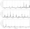 |
Fig. 4 Power spectrum of α Cen A. The frequencies in Table 2 are indicated with dotted lines. |
| In the text | |
|
Fig. 5 Collapsed échelle diagram. The first major peak, below 20μHz is an ℓ = 2 and the second, at 25μHz is an ℓ = 0. The two peaks around 65μHz belongs to the ℓ = 3 mode and the last peak, at 75μHz is an ℓ = 1. |
| In the text | |
|
Fig. 6 Echelle diagram of the new frequencies (black asterisks) and those reported by earlier studies: CORALIE (Bouchy & Carrier 2002) (blue squares), UVES-UCLES (Bedding et al. 2004) (red triangles), HARPS (Bazot et al. 2007) (green diamonds). |
| In the text | |
|
Fig. 7 Left panel: comparison of the large separation for ℓ = 0 modes with the one derived by Miglio & Montalbán (2005) in their models A3, with radiative core and A4, with convective core. Right panel: comparison of the small separation with the models A3 and A4. The agreement between the data points of our study and the models is significantly better than for the small separation obtained by Bouchy & Carrier (2002) (see Miglio & Montalbán 2005) |
| In the text | |
|
Fig. 8 Size of the splittings for ℓ = 1,2 and 3 modes, divided by 2m. The mean of these splittings should give the value of the rotation frequency of the star (see text). |
| In the text | |
|
Fig. 9 HR diagram showing the evolutionary tracks of model A3 (with a radiative core) and model A4 (with a convective core) from Miglio & Montalbán (2005). The error boxes for Teff, log L/L⊙, and radii correspond to 1σ (solid line) and 2σ (dashed-line). |
| In the text | |
|
Fig. 10 Left: comparison of the r02 constraint with the models A3 and A4. Right: comparison of the r10 constraint with the models A3 and A4. The data points seem clearly to agree with the model A3, a fact that was not established with the data of Bouchy & Carrier (2002). Indeed, all their points for the r10 asteroseismic constraint were situated between the curves of the models A3 and A4 (see Miglio & Montalbán 2005). |
| In the text | |
|
Fig. 11 Comparison of the δν13 constraint with the models A3 and A4. The model without overshooting is in a better agreement with the data than the model with overshooting. |
| In the text | |
Current usage metrics show cumulative count of Article Views (full-text article views including HTML views, PDF and ePub downloads, according to the available data) and Abstracts Views on Vision4Press platform.
Data correspond to usage on the plateform after 2015. The current usage metrics is available 48-96 hours after online publication and is updated daily on week days.
Initial download of the metrics may take a while.