| Issue |
A&A
Volume 523, November-December 2010
|
|
|---|---|---|
| Article Number | A73 | |
| Number of page(s) | 41 | |
| Section | Stellar structure and evolution | |
| DOI | https://doi.org/10.1051/0004-6361/201014763 | |
| Published online | 18 November 2010 | |
Deep infrared imaging of close companions to austral A- and F-type stars⋆,⋆⋆
1
Laboratoire d’astrophysique de Grenoble, Université Joseph Fourier, CNRS
(UMR 5571),
BP 53,
38041
Grenoble Cedex 9,
France
e-mail: This email address is being protected from spambots. You need JavaScript enabled to view it.
2
European Southern Observatory, Alonso de Cordova 3107, Vitacura Casilla 19001,
Santiago 19,
Chile
Received:
9
April
2010
Accepted:
24
June
2010
Abstract
The search for substellar companions around stars with different masses along the main
sequence is critical to understanding the different processes leading to the formation of
low-mass stars, brown dwarfs, and planets. In particular, the existence of a large
population of low-mass stars and brown dwarfs physically bound to early-type main-sequence
stars could imply that the massive planets recently imaged at wide separations (10–100 AU)
around A-type stars are disc-born objects in the low-mass tail of the binary distribution
and are thus formed via gravitational instability rather than by core accretion. Our aim
is to characterize the environment of early-type main-sequence stars by detecting
substellar companions between 10 and 500 AU. The sample stars are also surveyed with
radial velocimetry, providing a way to determine the impact of the imaged companions on
planets at ≲10 AU. High-contrast and high angular resolution near-infrared images of a
sample of 38 southern A- and F-type stars were obtained between 2005 and 2009 with the
instruments NaCo on the Very Large Telescope and PUEO on the Canada-France-Hawaii
Telescope. Direct and saturated imaging were used in the J to
Ks bands to probe the faint circumstellar environments with
contrasts of ~5 × 10⁻² to 10-4 at separations of
 and 1″, respectively. Using coronagraphic
imaging, we achieved contrasts between 10-5 and 10-6 at separations
>5″̣ Multi-epoch observations were performed to distinguish comoving companions
from background contaminants. This survey is sensitive to companions of A and F stars in
the brown dwarf to low-mass star mass regime. About 41 companion candidates were imaged
around 23 stars. Follow-up observations for 83% of these stars allowed us to identify a
large number of background contaminants. We report detection of 7 low-mass stars with
masses between 0.1 and 0.8 M⊙ in 6 multiple systems: the
discovery of an M2 companion around the A5V star HD 14943 and detection of HD 41742B
around the F4V star HD 41742 in a quadruple
system. We resolve the known companion of the F6.5V star HD 49095 as a short-period binary system composed of 2 M/L dwarfs. We also
resolve the companions to the astrometric binaries ι Crt (F6.5V) and 26 Oph (F3V), and identify an M3/M4 companion to the F4V star o Gru, associated with an X-ray source.
The global multiplicity fraction measured in our sample of A and F stars is ≥ 16%. This
has a probable impact on the radial velocity measurements performed on the sample
stars.
and 1″, respectively. Using coronagraphic
imaging, we achieved contrasts between 10-5 and 10-6 at separations
>5″̣ Multi-epoch observations were performed to distinguish comoving companions
from background contaminants. This survey is sensitive to companions of A and F stars in
the brown dwarf to low-mass star mass regime. About 41 companion candidates were imaged
around 23 stars. Follow-up observations for 83% of these stars allowed us to identify a
large number of background contaminants. We report detection of 7 low-mass stars with
masses between 0.1 and 0.8 M⊙ in 6 multiple systems: the
discovery of an M2 companion around the A5V star HD 14943 and detection of HD 41742B
around the F4V star HD 41742 in a quadruple
system. We resolve the known companion of the F6.5V star HD 49095 as a short-period binary system composed of 2 M/L dwarfs. We also
resolve the companions to the astrometric binaries ι Crt (F6.5V) and 26 Oph (F3V), and identify an M3/M4 companion to the F4V star o Gru, associated with an X-ray source.
The global multiplicity fraction measured in our sample of A and F stars is ≥ 16%. This
has a probable impact on the radial velocity measurements performed on the sample
stars.
Key words: stars: early type / binaries: close / surveys / astrometry / instrumentation: adaptive optics
Based on observations made with ESO Telescopes at the Paranal Observatory under programme IDs 076.C-0270, 081.C-0653, and 083.C-0151, and on observations obtained at the Canada-France-Hawaii Telescope (CFHT) which is operated by the National Research Council of Canada, the Institut National des Sciences de l’Univers of the Centre National de la Recherche Scientifique of France, and the University of Hawaii.
Appendices are only available in electronic form at http://www.aanda.org
© ESO, 2010
1. Introduction
Stars do not form alone, because they are often found in multiple systems that commonly consist of two or more stellar components, brown dwarfs, or planets. The various properties of these systems in terms of mass ratios and separations call for different formation mechanisms. At the lower end of the mass distribution, more than 400 extrasolar planets have been detected, most of them (~80%) with velocimetric surveys, and in most cases the planet-host stars are of solar type. This technique provided observational evidence that giant gaseous planets at separations ≲6 AU, which correspond to the largest revolution periods probed by radial velocimetry today, primarily form through rapid accretion of gas on pre-existing rocky cores, massive enough for triggering the runaway accretion of hydrogen (see, e.g., Mordasini et al. 2009). On the other hand, ~3% of the planets are detected by direct imaging searches at larger separations (≳ 10 AU), mainly around early-type stars. Most of these imaged planets seem to have a different origin: the fragmentation of the protoplanetary gaseous circumstellar disc (see, e.g., Dodson-Robinson et al. 2009; Kratter et al. 2010). Thus, there could be two possible paths of planet formation, depending on the stellar mass and planet separation.
The core-accretion theory (Pollack et al. 1996) is currently preferred to the gravitational instability theory (Boss 1997) as the origin mechanism of most planets detected by velocimetry, because the latter mechanism is not expected to produce giant planets at distances ≲10 AU (Rafikov 2005). Meanwhile, observational support has been gathered in favour of the core accretion theory. The correlation between the planet frequency and the host star metallicity (Santos et al. 2001, 2004) and the emerging fact that planets with an intermediate mass between Neptune’s and Saturn’s are exceedingly rare are both predicted in this theoretical frame. The recent extent of velocimetric surveys to low-mass main-sequence stars (M dwarfs; Mayor et al. 2009a,b) has yielded new key evidence in favour of this formation mechanism: for instance, that low-mass planets (about the mass of Neptune) are frequent, while gas giants are seldom found around low-mass stars observed by radial velocity or microlensing techniques (Bonfils et al. 2007; Sumi et al. 2010). In contrast, the frequency of giant planets should not be affected by the stellar mass in the frame of gravitational instability, as long as circumstellar discs are massive enough to become unstable (Boss 2006).
In fact, the total mass of the circumstellar disc where planets form is supposed to scale with the mass of the central star. An increase in the disc’s total mass can lead to an enhanced growth rate for protoplanetary cores in the disc midplane (Ida & Lin 2004), leading to a larger number of massive planets around early-type stars than around Sun-like stars. As a result, there should be an observational correlation between planet occurrence and stellar mass (Laughlin et al. 2004; Ida & Lin 2005; Kennedy & Kenyon 2007). Surveying early-type, main-sequence stars hotter and more massive than the Sun should allow such a correlation to be tested.
Radial velocimetry can be used to detect planets at short periods around main-sequence early-type stars, as shown by Lagrange et al. (2009a). These authors used the HARPS spectrograph installed at the ESO 3.6-m telescope in La Silla (Chile) to survey a sample of 185 stars. They measured the achievable detection limits on each star, taking the “jitter”1 level of each object into account. These authors estimated that planets with periods up to 100 days could be found around ~50% of the surveyed stars. Constraining the presence of planets at larger separations, however, requires a different detection technique.
In this respect, direct imaging is a powerful tool used as a complement to radial velocimetry for detecting companions at separations typically ≳10 AU. It is sensitive to intrinsically bright objects (low-mass stars, brown dwarfs, and young giant planets), and it brings essential insight to the possible origins of these objects (Chauvin et al. 2010). Direct near-infrared imaging allowed observers to detect several kinds of substellar companions, such as brown dwarfs (e.g., Nakajima et al. 1995; Lowrance et al. 1999, 2000; Chauvin et al. 2005a), objects at the transition between brown dwarfs and planets (e.g., Chauvin et al. 2005b), or planetary-mass objects such as 2M1207b in orbit around a brown dwarf (Chauvin et al. 2004, 2005c), all of which are probably not formed through core-accretion like planets detected by velocimetry, but rather as multiple stars via a cloud fragmentation process or as brown dwarfs through disc fragmentation (see, e.g., Lodato et al. 2005). These detections nevertheless show that star-forming mechanisms can be efficient down to planetary masses.
Recent breakthroughs in high-contrast imaging enriched this picture, as giant planets were directly imaged around Fomalhaut (Kalas et al. 2008), HR 8799 (Marois et al. 2008), and β Pictoris (Lagrange et al. 2009b, 2009c, 2010). All these stars are young and early main-sequence A stars. The discovery of a companion to β Pic, a 9 ± 3-MJ planet with a semi-major axis of ~8 to 15 AU, implies that giant planets can indeed form in ~10 Myr. According to the theoretical prediction of Kennedy & Kenyon (2007), this particular planet is close enough to its host star and could have formed in-situ by core accretion. This is not very clear for Fomalhaut b, which is located 115 AU away from its star, meaning that a particular migration scenario is required if the planet formed closer to the star via core accretion (Crida et al. 2009), or for the three planets or brown dwarfs located at 68, 38, and 24 AU from HR 8799. Gravitational instability, rather than core accretion, seems more suited to explaining the existence of such massive planets on wide orbits (Dodson-Robinson et al. 2009). The picture is, however, not that simple, as the gravitational instabilities leading to the fragmentation of massive circumstellar discs seem to produce objects with masses typically above the deuterium-burning planetary-mass limit. In fact, according to Kratter et al. (2010), atypical disc conditions are required to form planetary-mass object via this mechanism. These authors suggest that if these planets formed this way, they must lie in the low-mass tail of the disc-born binary distribution. In this case, more brown dwarfs or low-mass stars (such as M stars) should be found around A-type stars at distances of 50–150 AU.
In this framework, we perfomed a deep imaging survey of early-type A and F stars included in the velocimetric survey of Lagrange et al. (2009a). This study would allow us to test whether low-mass stars and brown dwarfs commonly cohabit with massive main-sequence stars, bringing new constraints on the origin of the massive planets imaged around these stars. In addition, this imaging survey could help in determining the impact of stellar multiplicity on the presence of closer-in planets, detected in parallel with radial velocimetry. Binarity is indeed another critical parameter for the theory of formation and evolution of planets. In particular, the separation of the binaries could affect the way giant planets form, either by core accretion or disc instability (Zucker & Mazeh 2002; Eggenberger et al. 2004; Desidera & Barbieri 2007; Duchêne et al. 2010), and the models of binary discs now predict observational effects. Mayer et al. (2005), for instance, predict a dearth of planets around each component of binary systems with separations ≲100 AU because of instabilities in the circumstellar discs. The subsequent dynamical evolution also depends on the properties of the star and the outer companion (see, e.g., Rivera & Lissauer 2000).
Only adaptive optics (AO) deep imaging allows proper testing for the presence of massive substellar companions. Several studies have previously been undertaken to probe the existence and the impact of such objects on exoplanetary systems detected by velocimetry (Patience et al. 2002; Luhman & Jayawardhana 2002; Chauvin et al. 2006, 2010; Mugrauer et al. 2007; Eggenberger et al. 2007). For instance, Eggenberger et al. (2007) have searched for bright long-period companions around 130 G- and K-type stars and measured a binary fraction of (8.8 ± 3.5)% in a subsample of 57 stars with planets detected with radial velocimetry at separations of 0″8–6″5 (i.e., 30–250 AU), whereas they found a higher binary fraction of (12.3 ± 3.2)% in a control subsample of 73 stars with no planet found. Previous works were also targeted on particular objects, such as Vega or ζ Virginis (Hinkley et al. 2010 and references therein), in search of substellar companions.
In this work, we focus on the close environment of a sample of austral A- and F-type stars, which we mainly observed from the southern hemisphere using the AO system NaCo installed at the ESO Very Large Telescope (VLT) on Cerro Paranal (Chile). Some austral stars were also observed from the northern hemisphere using PUEO, the AO bonnette of the Canada-France-Hawaii Telescope (CFHT) on Mauna Kea (USA). In a few cases, we also used NaCo to observe stars with positive declinations. This paper reports on these observations, which are described in Sect. 2. The data reduction is detailed in Sect. 3, and we present our analysis in Sect. 4 and discuss the results in Sect. 5.
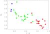 |
Fig. 1 Colours of stars in the imaging sample. Stars with spectral types F, A, and B are represented as red-, green-, and blue-filled circles, respectively. |
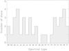 |
Fig. 2 Spectral types of the stars in the sample. |
2. Star sample and observations
2.1. Sample selection and biases
The present survey is the imaging part of the radial-velocity survey described in Lagrange et al. (2009a), which was designed to detect planets around early-type stars with the HARPS spectrograph at the ESO 3.6-m telescope in La Silla (Chile). The survey is limited to dwarfs with spectral types ranging from F7 to B82. Figure 1 presents the stars in a Hertzsprung-Russell diagram, while Fig. 2 shows the number of stars observed per spectral type. In total, we surveyed 38 stars, including 16 F-, 19 A-, and 3 late B-type stars.
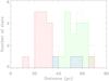 |
Fig. 3 Number of stars per 5-pc distance bin. The F, A, and B stars are represented by the histograms filled with tight diagonal red stripes, diagonal green stripes, and horizontal blue stripes, respectively. The dotted line stands for the whole star sample. |
The velocimetric and imaging surveys are also volume-limited, with distance limits set at 33 and 67 pc for the F0–F7 and B8–A9 dwarfs, respectively. Figure 3 gives the number of stars observed per 5-pc distance bin. The difference in distance limits would allow us to have roughly the same number of A and F stars in the sample; however, one early F star (HD 4293) with a distance of 66.6 pc is included in the survey.
Finally, the few stars present in our sample that are not included in the Lagrange et al. (2009a) sample are part of the northern radial-velocity survey in progress with the SOPHIE spectrograph (Bouchy et al. 2009) at the 1.93-m telescope in Observatoire de Haute-Provence (France). The properties of all stars in the sample can be found in Table 1. This table also gives the radial velocimetry status (“RV” column) of each object, as determined by Lagrange et al. (2009a) with HARPS or by Desort et al. (personal communication) with SOPHIE. The possible status are: constant (C), variable (V), with possible source of variations being spectral binary (SB), magnetic activity (A), pulsations (Pu), planets (Pl), or drift (D). Finally, the column “Multiplicity” of Table 1 indicates apparent (or comoving) binary (B), ternary (T), or more-component (M) systems, whether it is new (N) or known before this survey (K).
While more details about the sample selection are given in Lagrange et al. (2009a), we emphasize three biases. (i) First, spectroscopic binaries and close visual binaries with separations smaller than 5″ known at the beginning of the velocimetric survey were excluded from the target list. For this reason, these were not considered in the imaging survey. (ii) In addition, the present imaging survey is in fact strongly biased towards “interesting” targets, i.e., stars around which companion candidates (CC) were detected during early epochs. This strategy was set mainly in order to compensate for the limited amount of observing time devoted to the imaging programme. (iii) Finally, poor atmospheric conditions and technical problems that were experienced, especially during observing runs VI and VII, prevented us from obtaining second-epoch observations for 13% of those targets with companion candidate(s) identified during a first epoch. Atmospheric conditions making the AO correction loop unstable also prevented us from obtaining the highest achievable contrast – through the use of the coronagraph – for 10% of the targets.
2.2. Observations
Data were recorded during seven observing runs (or epochs) performed between January 2005 and August 2009, at the VLT and CFHT, where we totaled 7 + 8 nights of observations, respectively. The observing dates, instruments, and filters used during each epoch are summarized in Table 2, while the detailed observing set-ups for each target are given in Table 3.
2.2.1. VLT/NaCo
We used the NAOS-CONICA instrument (NaCo) set on the VLT Unit Telescope 4 (Yepun) to benefit from both the high image quality provided by the Nasmyth Adaptive Optics System (NAOS; Rousset et al. 2003) at infrared wavelengths and the good dynamics offered by the Near-Infrared Imager and Spectrograph (CONICA; Lenzen et al. 2003) detector, in order to study the close circumstellar environment of 38 early-type stars. The NaCo Shack-Hartmann visible wavefront sensor was chosen to perform the AO corrections on these bright targets, used as self-references. NaCo allowed us to perform both direct and coronagraphic imaging to improve the image contrast.
Star sample for the southern survey.
We used the coronagraphic mode consisting in a Lyot stop in the pupil plan of the
telescope, combined with an occulting mask of diameter  inserted in the focal plane. According to
the atmospheric conditions, we used different broad- and narrow-band filters whose
properties (central wavelength λc, bandpass
Δλ, and transmission T) are listed in Table 4. For instance, poor atmospheric conditions degrade
the Strehl ratio S. Using a long-wavelength filter (typically
Ks) can compensate for this degradation since the value of
S also scales with wavelength as
S = exp−(2πω / λ)2,
where ω is the root-mean-square deviation of the wavefront.
inserted in the focal plane. According to
the atmospheric conditions, we used different broad- and narrow-band filters whose
properties (central wavelength λc, bandpass
Δλ, and transmission T) are listed in Table 4. For instance, poor atmospheric conditions degrade
the Strehl ratio S. Using a long-wavelength filter (typically
Ks) can compensate for this degradation since the value of
S also scales with wavelength as
S = exp−(2πω / λ)2,
where ω is the root-mean-square deviation of the wavefront.
Epoch dates and astrometric calibrations for all observing runs.
Observing setups, dates, and number of companion candidates observed.
Two objectives were employed to optimize the point spread function (PSF) sampling in these different bandpasses. The S13 camera has a field of view of 14 × 14 arcsec2 and a mean plate scale of 13.21 mas pixel-1; it was preferred used when observing in J and H bands. When observing in the Ks band, the S27 camera was chosen. It offers a 28 × 28 arcsec2 field of view and a mean plate scale of 27.06 mas pixel-1. For each epoch, precise plate scales were redetermined using astrometric calibrators (see Table 2).
Our observing strategy consists, for each target, in obtaining a first-epoch image and, when companion candidates are detected, performing a second-epoch observation to test their status: either field objects (background contaminants) or comoving objects (physically bound to the targeted star). These two possibilities can be distinguished by the stellar proper and parallactic motions in the plane of the sky. This is illustrated in Fig. 4. Depending on motion amplitudes, a few months to a few years are necessary between the first- and second-epoch observations. For instance, for two observations performed three years apart and a precision on the measured positions of individual point sources on each epoch of ~10–20 mas (see Table 5), we can roughly estimate that a 3-σ discrimination between comoving and non-comoving sources is possible for typical minimum proper motions of ~15–30 mas yr-1.
A target is first observed both in direct imaging and coronagraphic modes. For epochs V, VI, and VII, the CoroObsAstro observing template was used. It consists in acquiring first some coronagraphic exposures on the object without any neutral density filter (Full_Uszd setting, where the pupil area is simply reduced by the Lyot stop, which blocks 14% of the light). Then, a neutral density filter (ND_Short) is inserted in the focal plane while removing both the coronagraphic mask and the Lyot stop in the focal and pupil plan, respectively. A direct image is then taken, with the object at the same exact location as behind the mask. This allows for retrieving the star position behind the mask, thereby enabling precise astrometric measurements of separation with companion candidates only visible in coronagraphic mode. The star is then jittered (by steps of ~5″) on 4 different locations on the detector to obtain the background sky estimation for the direct images. The last offset sends the telescope ~30″ away from the target star, and the occulting mask is used again – the neutral density filter is removed once more – as 5 jittered exposures are taken on the sky to estimate the sky background for coronagraphic images. This template was not available during our first NaCo observing run (epoch II), so the precise location of the star behind the mask is not known, and the astrometry is therefore less precise than for later observations. In all cases, the same amount of time was spent on the object and on the sky.
A systematic astrometric shift is induced when switching the neutral density filter back and forth: we used pinhole calibrations recorded at each epoch to ensure that this shift is small: typically ±0.1 pixel and ±0.01 pixel along the detector x- and y-axes, respectively. This shift is included in our error budget within the σs term of Eq. (1).
When a companion candidate can be detected without the coronagraph, the star is observed again at a later epoch, only in direct imaging mode. NaCo observing templates ImgGenericOffset and ImgAutoJitter were used for this purpose.
2.2.2. CFHT/PUEO
PUEO (Rigaut et al. 1998) is the AO bonnette mounted on the 3.6-m CFHT. It was used in combination with the near-infrared camera KIR (Doyon et al. 1998) with its field of view of 35 × 35 arcsec2 and a mean plate scale of 34.8 mas pixel-1. Depending on atmospheric conditions and source brightnesses, we used broad- and narrow-band filters listed in Table 4.
We performed unsaturated direct imaging to investigate as close as possible to the star, while the detector was saturated in order to increase the contrast at larger separations. (There is no occulting mask on PUEO.) Special care was taken to ensure that the unsaturated exposures could be used as references to measure the relative position and photometry between the star and the companion candidate(s). Images are jittered on the detector so that the sky background can be retrieved. The observing method is otherwise similar to the one described above for NaCo. The 6 stars from our sample with PUEO epochs have all been observed with NaCo, so are included in this study for consistency.
3. Data reduction
3.1. Calibrations
Flat fields were taken on the twilight sky for each observing run at VLT (usually within a few days from the observing nights). At CFHT, dome flat fields were taken for every filter at least once per run.
A well-known field in the Orion Trapezium centred on the star θ1 Orionis C was used for
astrometric calibrations (McCaughrean & Stauffer 1994). One observation per filter/camera set-up used was taken at each observing
epoch to determine the mean plate scale and the true north orientation. For each
observation, the exposure time was adjusted to saturate the 2 or 3 brightest stars of the
field so that from 15 to 40 stars (depending on the size of the field, from 13″ with the
S13 camera of NaCo to 35″ with PUEO) have a sufficient signal-to-noise ratio (≥ 5). The
position of the centroid
(sx,sy)
of each non-saturated star on the reduced image of the field is measured in pixels and
these values are then compared to the position on the sky
(ρx,ρy)
in arcseconds reported by McCaughrean & Stauffer (1994) with the following equations:
 where px
(py) is the plate scale along the
x- (y-) axis,
θn the orientation of the detector on
sky, and x0 and y0 are offsets
giving the correspondance between the absolute positions (only used to solve the
equation). A Levenberg-Marquardt minimization is then applied to find the plate scale
solution. The errors on the plate scale and orientation are given by the standard
deviation of the corresponding parameter. The mean plate scales and orientations are
reported in Table 2.
where px
(py) is the plate scale along the
x- (y-) axis,
θn the orientation of the detector on
sky, and x0 and y0 are offsets
giving the correspondance between the absolute positions (only used to solve the
equation). A Levenberg-Marquardt minimization is then applied to find the plate scale
solution. The errors on the plate scale and orientation are given by the standard
deviation of the corresponding parameter. The mean plate scales and orientations are
reported in Table 2.
3.2. Coronagraphic data
The reduction procedure makes use of the eclipse utility library (ESO 1996–2002; Devillard 1997). For each observing template on a target, coronagraphic exposures are sorted by eye. Good exposures (i.e., exposures where the star is well occulted and the AO correction loop is closed) are then concatenated into a data cube. A coronagraphic sky is created as the median of all dithered coronagraphic exposures on the sky, and is corrected twice for bad pixels detected (i) on the reduced flat field and (ii) on the median sky once the first bad-pixel rejection has been applied. The cleaned median sky is then subtracted to each plane of the data cube, which are next divided by the flat field. The 2 bad-pixel maps are again used on the flat-fielded data cube. The final reduced image is extracted as the median of the data cube.
3.3. Direct imaging data
The idea is similar to the reduction of data taken in coronagraphic mode, except that all the steps are performed by the jitter routine, which realigns dithered direct images via a cross-correlation algorithm and does all the cosmetic tasks. An additional (but similar) reduction is devoted to the first direct image taken after the coronagraph is removed (see Sect. 2.2.1), and this reduced image will be used as an astrometric reference for the position of the star behind the mask.
4. Analysis
4.1. Extraction of astrometric and photometric parameters of candidate companions
Candidate companions are spotted by a close eye-examination of each star, and their absolute position on the detector determined to a ~1-pixel precision. The position of the star is similarly estimated in unsaturated direct images from the astrometric direct images for coronagraphic observations. These positions are then used as input by a dedicated IDL wrapper programme that successively performs three astrometric and photometric estimations. (i) An aperture estimation, where the aperture is centred on the input position, returns the centroid position as the barycentre of the light within the aperture, and an arbitrary magnitude estimation from the integration of all pixels within the aperture, weighted by the flux of the reference PSF within the same aperture. The position (Δx,Δy) and magnitude Δm of each companion candidate are then given relative to those of the star. (ii) A Gaussian fitting using the IDL routine GCNTRD is also applied to each input position and returns relative separations. Finally, (iii) a deconvolution algorithm using a Levenberg-Marquardt minimization of the log-likelihood function (Véran 1997) is employed that basically consists in a PSF fitting within the pupil plane. Procedures (i) and (ii) work well when the objects are separated well on the image, and give similar results to procedure (iii). However, they do not give accurate results for tight systems (typically tighter than the aperture radius used). In these cases, our estimations rely on procedure (iii).
The astrometric precision is ultimately limited by the astrometric calibrator and by the
precision σp (in mas) obtained on the
estimation of the plate scale p (in mas pixel-1) at each epoch
(which are listed in Table 2). Nevertheless, our
procedure for extracting the astrometric parameters of an image is also characterized by
an uncertainty σs on the measured separation
s (both in pixels). The total uncertainty on the measured separation
ρ (in mas) is thus  (3)The values of
σs depend on various parameters such as the
actual separation of the components and their contrast. In the following, we choose to
take σs = 0.5 pixel as a conservative value.
In fact, this choice does not affect our conclusions concerning moderately separated
systems. Meanwhile, this value can be thought of as representative since it is clear that
the real precision we can achieve does not allow us to resolve the most difficult cases,
such as the very tight companion to HD 43940.
(3)The values of
σs depend on various parameters such as the
actual separation of the components and their contrast. In the following, we choose to
take σs = 0.5 pixel as a conservative value.
In fact, this choice does not affect our conclusions concerning moderately separated
systems. Meanwhile, this value can be thought of as representative since it is clear that
the real precision we can achieve does not allow us to resolve the most difficult cases,
such as the very tight companion to HD 43940.
Since the stellar flux is always estimated from the direct (unsaturated) image, both the direct and coronagraphic images are normalized by their respective exposure times when the photometry is performed for objects present in NaCo coronagraphic images. The magnitude difference is then increased by 4.6 mag to take the transmission difference introduced by the use of a neutral density filter into account. In the case of NaCo coronagraphic imaging, the use of a slightly undersized aperture caused by the Lyot stop in the pupil plan leads to an additional uncertainty of ~4% on the fluxes measured when the occulting mask is on, compared to the full aperture available when it is off (Boccaletti et al. 2007).
Properties of the filters used during the survey.
As for the separation, determining the contrast between two components is also affected by their respective brightnesses and separation. We can actually estimate our photometric precision from the set of dispersion of the measurements taken on the same objects at different epochs: the median dispersion obtained is 0.4 mag (45% on the measured fluxes). Astrometric and photometric measurements for all imaged companion candidates are given in Table 5. Stars without any detected companion candidates are listed in Table 6.
4.2. Companionship
The companionship, i.e., that a candidate companion is comoving with the primary star in
the vincinity of which it has been imaged – which is indicative of a physical association
bound by gravity – is appreciated by measuring the evolution of the separation
 and the position angle
θ = arctanΔx / Δy (from north to
east) between the candidate and the star over several epochs of observation. The values of
Δx and Δy are corrected for the orientation
θn of the detector north with respect to
the true north (given in Table 2 at each epoch).
The shift in the position (right ascension α and declination
δ) of a companion candidate between two epochs i and
j is
and the position angle
θ = arctanΔx / Δy (from north to
east) between the candidate and the star over several epochs of observation. The values of
Δx and Δy are corrected for the orientation
θn of the detector north with respect to
the true north (given in Table 2 at each epoch).
The shift in the position (right ascension α and declination
δ) of a companion candidate between two epochs i and
j is  These
measured shifts are compared to the theoretical apparent motion the object should have on
the sky, given the stellar proper motions listed in Table 1, the parallactic motion, and assuming, as is standard, that the candidate is a
motionless background contaminent. Figure 4 shows two
examples of companionship determination. The positions of all companion candidates
obtained during several observing runs are represented in Fig. A.1.
These
measured shifts are compared to the theoretical apparent motion the object should have on
the sky, given the stellar proper motions listed in Table 1, the parallactic motion, and assuming, as is standard, that the candidate is a
motionless background contaminent. Figure 4 shows two
examples of companionship determination. The positions of all companion candidates
obtained during several observing runs are represented in Fig. A.1.
For observations performed at N epochs, it is possible to calculate the
probability Pbkg that a companion candidate is a background
object, using a χ2 probability test of 2N−2
degrees of freedom: ![Mathematical equation: \begin{equation} \label{eq:chi2bkg} \chi^2_\mathrm{bkg} = \sum_{i=1}^{N} \left[ \frac{\left(\Delta\alpha_{1 \to i} - \Delta\alpha^\star_{1 \to i}\right)^2}{\sigma_{\Delta\alpha_{1 \to i}}^2 + \sigma_{\Delta\alpha^\star_{1 \to i}}^2} + \frac{\left(\Delta\delta_{1 \to i} - \Delta\delta^\star_{1 \to i}\right)^2}{\sigma_{\Delta\delta_{1 \to i}}^2 + \sigma_{\Delta\delta^\star_{1 \to i}}^2} \right], \end{equation}](/articles/aa/full_html/2010/15/aa14763-10/aa14763-10-eq135.png) (6)where
(6)where
 and
and
 are the theoretical shifts
in α and δ in the position of the star between epochs 1
and i, taking the stellar proper motion and the parallactic motion into
account.
are the theoretical shifts
in α and δ in the position of the star between epochs 1
and i, taking the stellar proper motion and the parallactic motion into
account.
The probability of observing a value of χ2 that is more than
obtained with Eq. (4) for a random sample
of N observations with ν = 2N−2
degrees of freedom is the integral of the probability density of a
χ2-distribution (Bevington & Robinson 2003),  (7)where
the Γ(n) function is equivalent to the factorial function
n ! extended to nonintegral arguments, and
(x2) represents the possible values of
χ2 within the integral sum. The probability
Pbkg is obtained from Eq. (5); practically speaking, we are using the IDL chisqr_pdf function. A
status of background contaminant is assigned to each object which
Pbkg > 0.01%. This probability is given for each
object in Fig. A.1. This first test allows rejecting
13 out of 41 detected point sources (32%), identified as background contaminants (labelled
“(B)ackground” in Table 5).
(7)where
the Γ(n) function is equivalent to the factorial function
n ! extended to nonintegral arguments, and
(x2) represents the possible values of
χ2 within the integral sum. The probability
Pbkg is obtained from Eq. (5); practically speaking, we are using the IDL chisqr_pdf function. A
status of background contaminant is assigned to each object which
Pbkg > 0.01%. This probability is given for each
object in Fig. A.1. This first test allows rejecting
13 out of 41 detected point sources (32%), identified as background contaminants (labelled
“(B)ackground” in Table 5).
Because of systematic effects on the position measurements, for instance, variations in
the stellar proper motions, discrepancies between the real values and those from the
literature, or the fact that background objects have a non-negligible
proper motion on the sky, we calculated Pbkg < 0.01%
for some objects that are evidently not comoving with the primary star. This is, for
instance, the case of HD 68456 CC#1 or HD 91889 CC#1 (see Fig. A.1). For this reason, we additionally define the probability
Pcmv, also given in Fig. A.1, that a companion candidate is comoving with the star, using a test similar
to Eq. (4), ![Mathematical equation: \begin{equation} \label{eq:chi2cmv} \chi^2_\mathrm{cmv} = \sum_{i=1}^{N} \left[ \left(\frac{\Delta\alpha_{1 \to i}}{\sigma_{\Delta\alpha_{1 \to i}}}\right)^2 + \left(\frac{\Delta\delta_{1 \to i}}{\sigma_{\Delta\delta_{1 \to i}}}\right)^2 \right]. \end{equation}](/articles/aa/full_html/2010/15/aa14763-10/aa14763-10-eq147.png) (8)The result is injected
into Eq. (5); however, the value of
Pcmvcan only be used to give a hint
of a physical association. In fact, this probability does not take the orbital
motion of a true comoving companion into account. An object with very small values of
Pbkg and Pcmv (<0.01%)
is therefore not necessarily a background contaminant because of orbital
motions.
(8)The result is injected
into Eq. (5); however, the value of
Pcmvcan only be used to give a hint
of a physical association. In fact, this probability does not take the orbital
motion of a true comoving companion into account. An object with very small values of
Pbkg and Pcmv (<0.01%)
is therefore not necessarily a background contaminant because of orbital
motions.
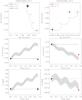 |
Fig. 4 Examples of the status determination of companion candidates around HD 14943 (left) and η Tuc (HD 224392; right), from astrometric measurements at two different epochs. The positions on the sky are reported in the upper panel: the candidates were first imaged on 2005-11-07 (filled black circles), then on 2008-08-20 (filled red and blue circles; there are two measurements in the case of HD 14943). The positions predicted for the candidates on 2008-08-20 if they were background objects from the field are indicated by the empty red and blue circles, and their trajectories between the two epochs figured by the black curves, which take the stellar proper motions and the parallactic motions into account. The middle and lower panels show the evolutions of the projected separations and the position angles, respectively, with time. One-sigma error bars are represented. A zero or near-zero evolution of the separation and position angle with time indicates a physical association. The candidate at the left is bound to its star with indicative probabilities Pbkg = 0% and Pcmv = 96.7% (following the calculations of Sect. 4.2), while the candidate at the right is a background contaminant, with Pbkg = 12.0% and Pcmv = 0%. |
Multi-epoch measurement results for 41 companion candidates detected around 23 stars of the sample.
Sample stars around which no companion candidates were detected.
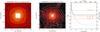 |
Fig. 5 Example of 6-σ detection limits reached for a K = 4.7 mag A0V star at 52.7 pc (HD 2834) using direct imaging (left panel) and coronagraphy (middle panel). Detection limits for the direct and coronagraphic image are given in 2 × 2 and 6 × 6 arcsec2 fields around the star, respectively. The hatched area on the coronagraphic image represents the occulting mask with a diameter of 0″̣7. Classic 1-dimensional 6-σ detection limits (right panel) are extracted from the direct image detection limit map (plain line) and the coronagraphy detection limit map (dotted line) as explained in Sect. 4.3. Mass limits (red lines) are obtained by interpolating Baraffe et al.’s (1998) evolutionary model for a given stellar age (here, 700 Myr). |
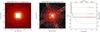 |
Fig. 6 Same as Fig. 5 for a K = 4.3 mag F7V star at 24.6 pc, and an age estimated to ~4.1 Gyr (HD 91889). |
Another tricky case is that of HD 41742 CC#1 (Pbkg = 0%, Pcmv = 0%), observed during 4 epochs. As can be seen in Fig. A.1 the second-epoch measurement is far from what is expected of a comoving object, and it is far from that of a background contaminant. Meanwhile, measurements recorded at all other epochs are very compatible with a comoving object (see HD 41742 CC#2 for comparison). This object is considered to be comoving because the measurement made during the second epoch for all three companion candidates to this star seem to be outliers. If we reject the measurements obtained at this epoch for this star, then CC#1 is comoving, while CC#2 and CC#3 indeed are background contaminants.
Finally, two point sources observed at several epochs continue to have an ambiguous nature (labelled “(A)mbiguous” in Table 5): HD 16555 CC#1, which is a true “in-between” case (see Fig. A.1), and HD 43940 CC#1, for the reasons developed in Sect. 4.4.2. The 13 other imaged point sources (32%) have only been observed once, so their status is set to “(U)ndefined” in Table 5.
4.3. Detection limits
For each image, we derived 6-σ detection limits in the form of a 2-dimensional map. The detection limits were calculated by measuring for each pixel the noise (standard deviation) in a 5 × 5 box centred on that pixel (see also Lagrange et al. 2009c). This operation was performed with the IDL routine IMAGE_VARIANCE (by M. Downing). The coronagraphic images were normalized to the exposure time of the associated direct image before their detection limits were calculated; the neutral density filter transmission was also taken into account. The classic 1-dimensional detection limits were then radially extracted from the 2D maps. The 1D detection limit at a separation ρ from the star position at (Δα,Δδ) = (0,0) is the azimuthal median of all pixels in an annulus of mean radius ρ with 5-pixel thickness.
These 1D detection limits can be used for determining the overall properties of our survey and comparing it to other surveys. However, since the contrast is mainly limited by the presence of speckles at close separations, we believe that the 2D maps are more accurate than the 1D limits and should instead be used when referring to particular objects in the survey. At large separations from the central stars, the contrast is fairly readout-noise limited, and both 1D or 2D limits could be used.
Figures 5 and 6 show the 2D- and 1D-detection limits achieved both in direct imaging and coronagraphic modes for two stars from our survey: an early A-type star (HD 2834; Fig. 5) and a late F-type star (HD 91889; Fig. 6) are chosen as typical examples. Maps of the detection limits for all surveyed stars are available in Appendix B. The overall 1D detection limits in the Ks band are presented in Fig. 7. Unlike the direct imaging observations, the coronagraphic imaging mode did not use a neutral density filter, thereby enabling improved sensitivities for wider-separation (greater than 2″) sources. With the coronagraph in place, we were able to employ large detector integration times (DITs), while still avoiding detector saturation. The larger DITs helped reduce detector read-out noise, which currently limits the wide-separation sensitivities. At separations over ~5″, we measured ~4-mag improvement between direct imaging and coronagraphic imaging modes.
Since the different spectral types of stars included in the survey have (i) different distance cut-off values (see Fig. 3) and (ii) different median ages, it is interesting to plot the overall detection limit for each spectral type (A, F, and B) as the median of all detection limits. Since there are only 3 B stars in the survey, the median limit for B stars cannot be considered as representative as for A and F stars.
Within this scope, the performance in contrast is slightly better, typically by
≲0.5 mag, for F-type stars than for A-type stars. Using direct-imaging mode, we achieve
typical contrasts of 4, 6, and 8.5 mag at 0″̣2,
0″̣5, and >1″ from the star,
respectively. The use of an occulting mask allows a better contrast than with direct
imaging from ~ . A maximum contrast of
~13 mag is reached at separations over 5″ from the star.
. A maximum contrast of
~13 mag is reached at separations over 5″ from the star.
4.4. Companion candidates detected
Companion candidates are detected at all separations above the detection limits. Table 5 presents the observing dates, integration times, projected separations, position angles, and magnitude differences of the 41 point sources we identified throughout our observing campaign. Based on the method presented in Sect. 4.2, we were able to determine that 20 objects (49% of sources detected) were background sources, and 6 objects (15% of sources detected) were in fact comoving with their primary stars. These confirmed companions are shown in Fig. 9 and their physical properties summarized in Table 7. Because a second-epoch observation could not have been obtained for all targets, 15 point sources are still undefined. In the following, we give the properties of all confirmed companions as well as those of a selection of remarkable cases of companions with undefinied status and some that we rejected as comoving objects.
4.4.1. Confirmed comoving companions
For companions comoving with their primary stars, the projected physical separation in astronomical units can be simply extracted from the knowledge of the separation measured on the sky and the parallax (usually, the Hipparcos parallax; ESA 1997). The masses of companions can be retrieved using mass-magnitude relationships coming from evolutionary models. The detection limits of our survey of A and F stars (Fig. 7) show that we are sensitive to companions in the brown-dwarf to low-mass star regimes. Thus, we chose the evolutionary models for solar-metallicity, low-mass stars and the associated mass-magnitude relationships provided by Baraffe et al. (1998) to determine the masses of our detected comoving companions. In practice, the masses were obtained for given absolute magnitudes and ages by interpolations into the Baraffe et al. tables (VizieR On-line Data CatalogueJ/A+A/337/403).
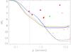 |
Fig. 7 Median 6-σ detection limits in the
Ks band for F- (red), A- (green), and B-type (blue)
stars, in direct imaging (plain lines) and coronagraphic (dashed lines) modes. The
coronagraphic detection limits are better than the direct imaging ones from 2″ on,
for the reasons given in Sect. 4.3. The
measured separations ρ and magnitude differences
ΔKs of companion candidates confirmed through
multi-epoch observations and those with an undefined status are indicated by
filled and empty circles, respectively. The confirmed companion candidate to
ι Crt, which was only observed in the H band,
is marked by the red square assuming a (H−K)
colour close to 0. The dash-dotted line at |

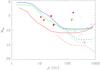 |
Fig. 8 Absolute magnitudes vs. projected separations. The legend is the same as for Fig. 7. The absolute magnitudes MKs and projected separations are calculated for each object given its apparent magnitude mKs in the Ks band and distance d from Earth. The 6-σ detection limits shown for F- (red), A- (green), and B-type (blue) stars in direct imaging (plain lines) and coronagraphic (dashed lines) modes are the medians of the detection limits MKs = f(ρ(d),d,mKs) calculated for all stars of a given spectral type. |
Physical properties of comoving companions.
HD 14943 –
A companion with an absolute magnitude of
MK = 6.6 mag has been identified at two
different epochs  (141 AU) away from
the A5V star HD 14943 (HIP 11102). According to the Baraffe et al. (1998) evolutionary models for solar-metallicity,
low-mass stars, this companion should be a 0.4 M⊙ star,
assuming an age of 850 Myr, determined in the frame of the Su et al. (2006) survey of debris discs around A stars with
Spitzer/MIPS. For this reason, HD 14943B, shown in Fig. 9a, could be a main sequence M2 star (Cox 2000)3.
(141 AU) away from
the A5V star HD 14943 (HIP 11102). According to the Baraffe et al. (1998) evolutionary models for solar-metallicity,
low-mass stars, this companion should be a 0.4 M⊙ star,
assuming an age of 850 Myr, determined in the frame of the Su et al. (2006) survey of debris discs around A stars with
Spitzer/MIPS. For this reason, HD 14943B, shown in Fig. 9a, could be a main sequence M2 star (Cox 2000)3.
HD 41742 –
This high proper-motion star is part of a physical ternary hierarchical system
(Multiple Star Catalogue – MSC –, Vizier Online Data Catalogue J/A+AS/124/75,
Tokovinin 1997). We identified CC1 to component
B (CCDM J06046-4504B; see Fig. 9b), a
0.79 M⊙ star with a period of ~1400 yr. The
mass given in the MSC was determined from the measured
B−V = 1.01, typical of a K0/K2 star according to
Cox (2000). The two other companion candidates
(CC2 and CC3) are background objects. The component C of the system catalogued in the
MSC is too far to enter the NaCo or PUEO field-of-view ( ). Furthermore, the
primary star has been shown to be a spectroscopic binary according to the radial
velocity curves obtained by (Lagrange et al. 2009a). The imaged companion is not responsible for the radial velocity
variations, making HD 41742 a member of a quadruple system. We measured for HD 41742B
(CC1) a projected separation of 5″̣9, i.e., 159 AU and an absolute
magnitude MK = 4.0 mag, which translates
into a 0.8-M⊙ star using the Baraffe et al. (1998) mass-magnitude relationships, in good
agreement with the mass previously determined. This estimation was made assuming an
age of 3.7 Gyr, according to the Geneva-Copenhagen Survey of Solar Neighbourhood
(GCSSN, Vizier Online Data Catalogue V/130, Holmberg et al. 2009).
). Furthermore, the
primary star has been shown to be a spectroscopic binary according to the radial
velocity curves obtained by (Lagrange et al. 2009a). The imaged companion is not responsible for the radial velocity
variations, making HD 41742 a member of a quadruple system. We measured for HD 41742B
(CC1) a projected separation of 5″̣9, i.e., 159 AU and an absolute
magnitude MK = 4.0 mag, which translates
into a 0.8-M⊙ star using the Baraffe et al. (1998) mass-magnitude relationships, in good
agreement with the mass previously determined. This estimation was made assuming an
age of 3.7 Gyr, according to the Geneva-Copenhagen Survey of Solar Neighbourhood
(GCSSN, Vizier Online Data Catalogue V/130, Holmberg et al. 2009).
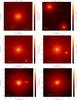 |
Fig. 9 Stars with companion candidates confirmed through multi-epoch observations. North is up and east to the left. Counts on the detector are displayed with a logarithmic scale. |
HD 49095 –
This high proper-motion star with radial velocity variations (Lagrange et al. 2009a) is referred to as a binary by Makarov & Kaplan (2005) based on the difference in proper motions measured between two different catalogues (“Δμ binary”), Hipparcos and Tycho-2. Here, we image the binary component and resolve it as a tight binary in which orbital motion is detected over several epochs. The system is shown as seen on 2005-11-07 in the Ks band with NaCo in Figs. 9c and 10, and the revolution of the B (CC1) and C (CC2) components around their centre of mass is shown over 3.5 years (4 epochs) in Fig. C.1. The position of HD 49095C with respect to HD 49095B was retrieved using the deconvolution algorithm described in Sect. 4.1 and is plotted in Fig. 11. For the two VLT images (taken on 2005-11-07 and 2009-04-26) where the HD 49095BC system is fully resolved, we assumed 1-σ position errors of 0.25 pixel. A position error of 0.5 pixel has been assumed for CFHT images (taken on 2007-01-27 and 2007-11-26) where the system is barely resolved. The tight system projected separation is seen to vary between 1.4 and 2.6 AU; and yet, because we do not have enough points to fit a precise orbit, we simply calculated a best-fit circular orbit, assuming the system is seen face-on, and determined a semi-major axis of 2.27 AU (χ2 = 3.3 with 1 degree of freedom). HD 49095C accomplishes roughly 60% of this circular orbit in 3.5 yr, which leads to a revolution period of 5.7 yr. Using Kepler’s third law, we can then determine a total mass for the BC system of 0.11 M⊙. This is about three times lower than the total mass determined photometrically using the Baraffe et al. (1998) models (0.175 + 0.13 = 0.305 M⊙) given the measured magnitudes in the H band of MHB = 8.5 and MHC = 9.0 mag and the age of 2 Gyr provided by the GCSSN. We attribute this discrepancy to the orbit not being well constrained with 4 epochs.
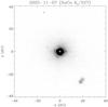 |
Fig. 10 The F6.5V star HD 49095 and its binary comoving companion composed of CC1 (blue circle) and CC2 (red circle). The axes are labelled in projected separation with respect to the primary star centroid position (white star). The positions of objects on this image are retrieved using the deconvolution algorithm described in Sect. 4.1. |
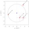 |
Fig. 11 Motion of the binary companion CC2 of HD 49095 (zoom from Fig. 10) relative to CC1 (blue point) between 4 different epochs covering 3.5 yr. The best-fit circular and face-on orbit is depicted, with a semi-major axis of 2.27 AU. |
HD 101198 –
The ι Crateris (HD 101198; CCDM J11387-1312A) entry in the CCDM
mentions a companion (KUI 58B) at  and
θ = −134° in 1934, with a visual magnitude
V = 11. The star is recorded as a probable single star in the Double
and Multiple Systems Annex of the Hipparcos Catalogue (ESA 1997), yet Makarov
& Kaplan (2005) as well as Frankowski
et al. (2007) see it as a Δμ
binary. Were KUI 58B a background contaminant, it would lie in 2009 at
and
θ = −134° in 1934, with a visual magnitude
V = 11. The star is recorded as a probable single star in the Double
and Multiple Systems Annex of the Hipparcos Catalogue (ESA 1997), yet Makarov
& Kaplan (2005) as well as Frankowski
et al. (2007) see it as a Δμ
binary. Were KUI 58B a background contaminant, it would lie in 2009 at
 and
θ ≈ −141deg, so that we should be able to detect it in NaCo
Ks images, unless its
V−K colour index is below ~− 1.5.
The other possibility is that KUI 58B is indeed bound to ι Crt. In
this case, it is likely that CC1, shown in Fig. 9d, is that object. This would imply colour indexes
V−K ≈ 11−7.25 = 3.75 and
V−H ≈ 11−7.44 = 3.56 for CC1, typical of an M3
dwarf (Ducati et al. 2001)4. The mass derived from the measured
MH = 5.2 mag using evolutionary model
and assuming an age of 4.8 Gyr (from the GCSSN) is
0.57 M⊙, more typical of an M0 or a late K star (Cox 2000). Furthermore, the primary shows radial
velocity variations (Lagrange et al. 2009a).
and
θ ≈ −141deg, so that we should be able to detect it in NaCo
Ks images, unless its
V−K colour index is below ~− 1.5.
The other possibility is that KUI 58B is indeed bound to ι Crt. In
this case, it is likely that CC1, shown in Fig. 9d, is that object. This would imply colour indexes
V−K ≈ 11−7.25 = 3.75 and
V−H ≈ 11−7.44 = 3.56 for CC1, typical of an M3
dwarf (Ducati et al. 2001)4. The mass derived from the measured
MH = 5.2 mag using evolutionary model
and assuming an age of 4.8 Gyr (from the GCSSN) is
0.57 M⊙, more typical of an M0 or a late K star (Cox 2000). Furthermore, the primary shows radial
velocity variations (Lagrange et al. 2009a).
HD 153363 –
26 Ophiuchi (HD 153363) is referred to as a radial-velocity variable (Lagrange et al. 2009a) as well as an astrometric binary (Proper motion derivatives of binaries, Vizier Online Data Catalogue J/AJ/129/2420, Makarov & Kaplan 2005; HIP binaries with radial velocities, Vizier Online Data Catalogue J/A+A/464/377; Frankowski et al. 2007), and yet no orbit information is available in the litterature. The binary component expected by astrometric measurements could well be CC1. In fact, we determined that the motion of CC1 seen between August 2008 and April 2009 cannot be due to the combination of the stellar proper motion and the parallactic motion, which are for this low-proper motion star of similar amplitudes. It can be seen in Fig. A.1 that the position of CC1 in April 2009, imaged in Fig. 9e, is not compatible with that of a background field object, so the motion of CC1 can instead be explained by the orbital motion around 26 Oph. We observed 26 Oph B in three band passes and measured ΔKs = 2.1, ΔH = 2.7, and ΔJ = 3.1. Given the 2MASS JHK magnitudes of 26 Oph and its distance of 33.3 pc, the companion has absolute magnitudes MKs = 4.2, MH = 4.9, and MJ = 5.5. These magnitudes are compatible, within the given uncertainty range of ± 0.4 mag, with a 1.0–1.3-Gyr-old 0.7-M⊙ object according to the Baraffe et al. (1998) model. Assuming the J−Ks and H−Ks colours are each overestimated by ~0.4 mag (a 1-σ variation), they indeed correspond to the colours of an early K dwarf (Ducati et al. 2001). Additional fainter and farther components of this system may exist. Only the two brightest companion candidates are reported. Many other point sources (~56) are seen using the coronagraph; however, they are all likely background contaminants as the star is close to the Galactic plane (b = + 10.6°). Besides, we miss a second epoch observation with the coronagraphic mask. Meanwhile, we can already exclude CC2, also seen in the direct images, as an additional physical companion to 26 Oph.
HD 220729 –
Lagrange et al. (2009a) identified o Gruis (HD 220729) as a spectroscopic binary and noted that it was associated to a ROSAT source by Suchkov et al. (2003). In this work, we confirm the binary nature of this star since we resolve it as a tight (0″̣4 or 14.9 AU) and contrasted (ΔK = 4.7) binary system, as can be seen in Fig. 9f. We estimate the absolute magnitude of o Gru B to MK = 6.7 for an age of 1.1 Gyr (GCSSN), which yields a mass of 0.3 M⊙, i.e., an M3/M4 main sequence star. The companion detected in the adaptive-optics survey is not responsible for the radial-velocity shifts, meaning that o Gru is a triple system.
4.4.2. Companion candidates with undefined or ambiguous status
HD 32743 –
η1 Pictoris (HD 32743, HIP 23482) is catalogued in the
CCDM as a binary with an astrometry recorded in 1946 of  and
θ = −162° and a photometry of ΔV = 7.4 mag. (No
associated uncertainties on these parameters are reported.) We observed this object
during a single epoch on 2005-11-07 and obtained the following astrometry for CC1:
and
θ = −162° and a photometry of ΔV = 7.4 mag. (No
associated uncertainties on these parameters are reported.) We observed this object
during a single epoch on 2005-11-07 and obtained the following astrometry for CC1:
 and
θ = −176.32 ± 0.12°. We measured infrared apparent magnitudes of
J = 12.6 (ΔJ = 7.8) and
Ks = 11.8 (ΔKs = 7.4) for
CC1, which seem compatible with the visible apparent magnitude
(V = 13) of the known companion to
η1 Pic. It is therefore likely that CC1 is the binary
companion to η1 Pic and catalogued as CD-49 1541B. To estimate whether CC1 is comoving with
η1 Pic, we produced a proper motion plot similar to
those of Fig. A.1 as presented in Fig. D.1. We assumed arbitrarily large error bars on the
1946 astrometric parameters tabulated in the CCDM. The position of the object measured
in 2005 corresponds to that of a background object, not comoving with the primary
star. We obtain Pbkg = 24.9%. The lack of reported
uncertainties in the CCDM does not allow a firm conclusion on the companionship status
of CC1/CD-49 1541B, but we consider it as a probable background contaminant. We
nevertheless resolve it as a tight apparent binary (ρ,
θ, and Δm of the three other companion candidates
have been determined with respect to the properties of CC#1, which is seen both in
direct and coronagraphic images), and since a second tight binary system is also
present in the surroundings of η1 Pic, the system will
need to be monitored in the future.
and
θ = −176.32 ± 0.12°. We measured infrared apparent magnitudes of
J = 12.6 (ΔJ = 7.8) and
Ks = 11.8 (ΔKs = 7.4) for
CC1, which seem compatible with the visible apparent magnitude
(V = 13) of the known companion to
η1 Pic. It is therefore likely that CC1 is the binary
companion to η1 Pic and catalogued as CD-49 1541B. To estimate whether CC1 is comoving with
η1 Pic, we produced a proper motion plot similar to
those of Fig. A.1 as presented in Fig. D.1. We assumed arbitrarily large error bars on the
1946 astrometric parameters tabulated in the CCDM. The position of the object measured
in 2005 corresponds to that of a background object, not comoving with the primary
star. We obtain Pbkg = 24.9%. The lack of reported
uncertainties in the CCDM does not allow a firm conclusion on the companionship status
of CC1/CD-49 1541B, but we consider it as a probable background contaminant. We
nevertheless resolve it as a tight apparent binary (ρ,
θ, and Δm of the three other companion candidates
have been determined with respect to the properties of CC#1, which is seen both in
direct and coronagraphic images), and since a second tight binary system is also
present in the surroundings of η1 Pic, the system will
need to be monitored in the future.
HD 43940 –
Clearly seen in 2005-November observations in the Ks
band, the close companion candidate to HD 43940 ( ) is harder to
resolve from the primary star in 2008-August, in both Ks
and H bands. This may be due, however, to the poorer observing
conditions compared to 2005 November. A final attempt to characterize this new tight
system was made on 2009 April, but the companion could barely be resolved from the
primary star in the J band. HD 43940 has very low proper motions in
the direction of CC1
(δα = −5.51 mas yr-1,
δδ = −22.63 mas yr-1), but
since the separation is small, it is hard to distinguish between the two
possibilities: (i) the system is apparent and CC1 is a nearly motionless background
contaminant apparently getting closer to HD 43940 because of this star proper motions;
or (ii) the system is physically bound and the difficulty to resolve it as time passes
results from the orbital motion of CC1 around the primary.
) is harder to
resolve from the primary star in 2008-August, in both Ks
and H bands. This may be due, however, to the poorer observing
conditions compared to 2005 November. A final attempt to characterize this new tight
system was made on 2009 April, but the companion could barely be resolved from the
primary star in the J band. HD 43940 has very low proper motions in
the direction of CC1
(δα = −5.51 mas yr-1,
δδ = −22.63 mas yr-1), but
since the separation is small, it is hard to distinguish between the two
possibilities: (i) the system is apparent and CC1 is a nearly motionless background
contaminant apparently getting closer to HD 43940 because of this star proper motions;
or (ii) the system is physically bound and the difficulty to resolve it as time passes
results from the orbital motion of CC1 around the primary.
HD 158094 –
The B8 star δ Aræ (HD 158094) is part of an optical (Torres 1986) double system (CCDM 17311-6041) whose
secondary component lies outside the field of view ( ,
θ = 313°). Spitzer/MIPS 24-μm
photometry indicates an age of 125 Myr for the star itself and nonexistent infrared
excess (Rieke et al. 2005). Low-mass companions
were searched for around this star by Hubrig et al. (2001) using the AO system ADONIS on the ESO 3.6-m telescope in La Silla.
These authors report detection limits of ΔK ~ 5 mag for a
separation of ~2″–5″ and ΔK ~ 9 for ≳4″̣ This
means CC3 (
,
θ = 313°). Spitzer/MIPS 24-μm
photometry indicates an age of 125 Myr for the star itself and nonexistent infrared
excess (Rieke et al. 2005). Low-mass companions
were searched for around this star by Hubrig et al. (2001) using the AO system ADONIS on the ESO 3.6-m telescope in La Silla.
These authors report detection limits of ΔK ~ 5 mag for a
separation of ~2″–5″ and ΔK ~ 9 for ≳4″̣ This
means CC3 ( ,
θ = 62.0°, ΔK = 8.2) could have been detected by
Hubrig et al. (2001): it is slightly above
their detection limit, and close to the edge of, yet within, their 24″ × 24″ field of
view, centred on the star, in 1999 March. If CC3 were a background contaminant, then
it would have been closer to star in 1999 (
,
θ = 62.0°, ΔK = 8.2) could have been detected by
Hubrig et al. (2001): it is slightly above
their detection limit, and close to the edge of, yet within, their 24″ × 24″ field of
view, centred on the star, in 1999 March. If CC3 were a background contaminant, then
it would have been closer to star in 1999 ( ) given the star
proper motion.
) given the star
proper motion.
4.5. Notes on some remarkable non-comoving multiple systems
HD 3003 –
β3 Tucanæ (HD 3003) was previously known as a multiple star (CCDM J00327-6302AB). Were this system comoving, we should be able to retrieve both components, separated by 6″̣4 in 1925 (as tabulated in the CCDM). Only one star is visible in the 2005 NaCo image, so this system is only a visual assocation.
HD 50445 –
The star HD 50445 is not catalogued as part of a multiple apparent or physical system.
However, it lies at a relatively low Galactic declination
(b = −15.6°), and at least 5 point sources have been detected in
2005-November in the 27″-wide field of NaCo S27 camera, using the coronagraphic mask.
All 5 objects were observed again in 2009 April, but a software problem during the
observations unfortunately prevented recording a direct image of the primary star at
this epoch. This makes the astrometric precision lower for the 2009 observations
(typically 1 pixel, i.e., 30 mas). We are nevertheless confident that all candidate
companions are background contaminants. Companion candidate #2 can be seen in the
infrared Digitalized Sky Survey 2 image taken on 1985 December at
ρ ~ 14″ and θ ~ 155°. (The apparent
motion of the background contaminants on the sky between 1985 and 2005 is
 and
and  .)
.)
HD 177756 –
λ Aquilæ (HD 177756) is one of the B stars included in the Hubrig et al. (2001) survey. These authors did not report any companions in the K band with a magnitude difference up to ΔK ~ 9. The observed CC1 has a magnitude difference of ΔK = 4. It should have been seen in the 1999 ADONIS image, as this background contaminant was closer to the star at this epoch, unless the field of view of 24″ × 24″ reported by Hubrig et al. is not squarred (depending on the dithering pattern used by these authors).
HD 216385 –
This star has two companion candidates. The first one (CC#1) is not seen in the second-epoch observation, while CC#2 is too weak to have been detected during the first PUEO epoch. It was, however, outside the field of a third NaCo epoch not reported in Table 5 and is thus a likely background contaminant.
HD 224392 –
Members of the Tucana association, including the Vega-like star η Tucanæ (HD 224392; see Mannings & Barlow 1998 for the infrared excess), were surveyed in the infrared by Neuhäuser et al. (2003) with the SHARP-I infrared imager on the New Technology Telescope (NTT) at La Silla. These authors report detection limits in the K band of ΔK = 8.3 at >100 AU from the star. However, they could not have detected CC1 because it was out of SHARP-I 13″ × 13″ field-of-view. Zuckerman et al. (2001) note that as part of the IRAS Faint Source Catalogue (Vizier online data catalogue II/156A; Moshir 1989), η Tuc might also be a multiple star, yet in this case we do not resolve it. Besides, being a HARPS constant (Lagrange et al. 2009a) makes it unlikely to be a spectroscopic binary. We do detect two companion candidates far from the star, which are not comoving with it.
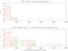 |
Fig. 12 Number of detected companions as a function of the projected separation to the primary, per bin of 100 AU. Companions around F stars (red stripes) and A+B stars (green stripes) are differenciated. The black dotted line represents the total number of companions. (a) Confirmed companions only. (b) Confirmed and unconfirmed companions. |
5. Discussion
5.1. Multiplicity of early-type stars in the sample
We found that 6 stars out of 38 in the sample have confirmed low-mass companions, yielding an observed multiplicity fraction of 16% for our sample. This number can be seen as a lower limit value for the sample (i) because we have imaged companion candidates around 7 other stars in the sample, without having the possibility of determining whether they are true companions or background objects; (ii) because we could have missed close binaries below our detection limits; and/or (iii) because some wide-separation binary components could have been too close to the line of sight to be resolved at the time of observations. It is also most certainly a lower limit value regarding the global multiplicity fraction of early-type stars, since our survey is biased against spectral binaries or visual binaries with companions at ≤5″, as described in Sect. 2.1.
When all the undefined candidates are bound to their primary stars, the multiplicity fraction of sample stars can be as high as 34%. More specifically, the multiplicity fraction for F stars in the sample is 5 / 16 ≈ 31% and 1 / 22 ≈ 5% for A+B stars. If we assume that unconfirmed companions are all physically bound companions, then these fractions rise to 50% and 23% for F and A+B stars, respectively. The multiplicity fraction could even be higher than these figures owing to narrow-separation binaries and orbital projection effects.
Considering confirmed companions alone, it would seem surprising that the multiplicity fraction of F stars is 6 times more than for A stars, whereas it is usually expected that the multiplicity fraction increases with the stellar mass. Actually, this is a bias that can be attributed to our probing different physical separations for different stellar types. To have about the same number of F and A stars included in this volume-limited survey, we have to go further and including as many A stars as F stars: the median distance of sample F stars is 27.0 pc, while it is 54.9 pc for sample A and B stars (see Fig. 3). Thus, we are probing smaller physical separations for F stars than for A and B stars, as shown in Fig. 7b. Five out of 6 confirmed companions detected next to F stars are located between 10 and 40 AU, at projected separations hardly reached for the A stars in the sample or not reached at all. In contrast, a confirmed companion located at >100 AU was found for each type of stars.
Figure 12 shows the number of confirmed companions (Fig. 12a) or confirmed and unconfirmed companions (Fig. 12b) per bin of 100 AU from their primary stars. The bias is clearly apparent in Fig. 12a if we assume that our detection efficiency at <100 AU is lower for A stars than for F stars. If we further assume that all unconfirmed companions are physically bound to their primary stars, then Fig. 12b shows that we have roughly the same number of objects between 100 and 500 AU, while companion candidates at projected distances greater than 500 AU are only found around A+B stars. It is likely that at least some unconfirmed objects detected around A stars are real companions, and contribute with the observational bias to filling the gap between the multiplicity fractions of A and F stars in the sample.
5.2. Impact of imaged companions on the velocimetric survey
The objects from the imaging survey presented in this work have been – or are being – monitored spectroscopically, seeking for radial velocity variations that would reveal the presence of close-in companions (see Lagrange et al. 2009a). Two questions arise when companions are imaged around stars included in the velocimetric survey.
First, is the spectroscopic signal contaminated by a companion that would appear blended
with the primary star in the spectrograph fiber? All background objects detected in the
imaging survey are far enough from their stars and do not enter the fiber
(⌀ ~ 2″) used in the velocimetric survey. Thus, they do not pollute the radial
velocity signal. On the contrary, the companion candidate to HD 43940 (ambiguous case) probably contributes to the velocimetric signal.
Six of the seven comoving companions detected, HD 14943B ( ), HD 49095BC
(
), HD 49095BC
( ), ι Crt B
(
), ι Crt B
( ), 26 Oph B (
 ), and
o Gru B (
), and
o Gru B ( ), are close enough to their stars to directly
contribute to the spectroscopic signal. Note that o Gru B probably
marginally pollutes the velocimetric signal depending on seeing conditions. However, the
contribution in terms of flux is generally limited given the flux ratios between the stars
and the companions.
), are close enough to their stars to directly
contribute to the spectroscopic signal. Note that o Gru B probably
marginally pollutes the velocimetric signal depending on seeing conditions. However, the
contribution in terms of flux is generally limited given the flux ratios between the stars
and the companions.
On the other hand, are the radial velocity variations a result of the gravitational perturbations of the imaged companions? Indeed, all the 6 stars for which we imaged and confirmed a companion are reported with velocimetric variations in Lagrange et al. (2009a). Radial velocity curves (Lagrange et al. 2009a) indicate that two of them (HD 41742 and o Gru) belong to multiple systems, and this includes a spectroscopic binary surrounded by a wider-separation companion, detected only with adaptive optics5. The imaged companions are not responsible for the radial velocity variations in these cases. Meanwhile, the confirmed companions around the four other stars partly or totally contribute to the radial velocity variations observed by Lagrange et al. (2009a, and in prep.). In the ambiguous cases of HD 43940 and η Hor, the companion candidates could contribute to the observed radial velocity variations, if they are bound objects.
In either case, this shows that the radial velocity curves of at least 6 out of 35 stars followed spectroscopically (17%) may be affected by stellar multiplicity.
6. Conclusions
We have presented a deep imaging near-infrared survey of 38 austral early-type main
sequence stars, searching for low-mass companions at intermediate distances. The overall
detection performances obtained for this survey, mainly performed in the
K band at 2.2 μm, allowed us to probe the stellar
environments at separations > with contrasts <0.05. Farther from the
stars (>5″), we achieved limiting contrasts between 10-5 and
10-6 using coronagraphy. Although known binary stars were excluded from the
survey, we detected 41 companion candidates around 23 stars. Using multi-epoch observations,
we were able to determine that 7 candidates are actually comoving companions around 6 stars
of the sample, while the other candidates are mainly background contaminants. The comoving
companions are low-mass stars with masses ranging from 0.13 to
0.8 M⊙. A comoving binary system consisting of 2 M/L dwarfs
imaged around HD 49095, with an almost fully resolved orbit, will be of particular interest
for calibrating low-mass star evolution models. The comoving companions are detected at
projected separations ranging from 11.3 to 159 AU.
At least 16% of the sample stars, with spectral types ranging from F7 to B9, therefore host a low-mass star companion. This figure is likely a lower limit to the real multiplicity fraction of early-type stars within this separation range. In addition, all the detected and confirmed companions have projected separations below 200 AU: this range matches the physical projected separations of giant planets recently imaged in discs surrounding A-type stars Fomalhaut and HR 8799 (Kalas et al. 2008; Marois et al. 2008). It is certainly tantalizing to interpret the emerging population of such massive planets as the low-mass tail of the binary distribution of early-type stars. This would imply that these planets are formed by gravitational instability rather than core accretion like closer-in planets. However, further evidence from larger, less-biased surveys is still required to assess this question in a statistical and quantitative fashion.
Most stars of our sample are also included in spectroscopic surveys (Lagrange et al. 2009a) seeking for radial velocity variations. Crossing the results of both surveys shows that at least 17% of the radial velocity curves may be affected by companions detected with adaptive optics.
We finally emphasize that tight stellar systems with a bright early-type primary component, such as the ones presented in this study, will be excellent calibrators for next-generation planet imagers such as VLT/SPHERE or interferometers like VLT/Gravity, designed for high-precision astrometry within small field-of-views.
Online material
Appendix A: Companion candidates motions on the sky
The astrometric measurements for all point sources detected at several observing epochs are represented in Fig. A.1. The background/comoving probabilities defined in Sect. 4.2 are given over each panel.
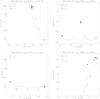 |
Fig. A.1 Motions of companion candidates measured on the sky relatively to their respective primary stars (at (Δα,Δδ) = (0,0)). The theoretical motion of an object is calculated from its initial first epoch measurement (black filled circle) assuming it is a background contaminant and given the proper and parallactic motions of the primary star (black curve), for the different epochs where measurements have been recorded (empty circles). The measured positions for these different epochs are reported (filled circles) for comparison. When the measurements (filled circles) agree with the theoretical motion path, the companion candidate is likely a background contaminant. |
 |
Fig. A.1 continued. |
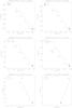 |
Fig. A.1 continued. |
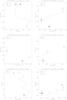 |
Fig. A.1 continued. |
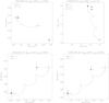 |
Fig. A.1 continued. |
Appendix B: Detection limits for all stars
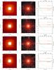 |
Fig. B.1 Detection limits in the Ks band. |
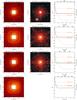 |
Fig. B.1 continued. |
 |
Fig. B.1 continued. |
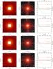 |
Fig. B.1 continued. |
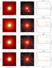 |
Fig. B.1 continued. |
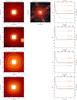 |
Fig. B.1 continued. |
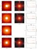 |
Fig. B.1 continued. |
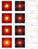 |
Fig. B.1 continued. |
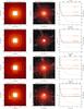 |
Fig. B.1 continued. |
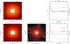 |
Fig. B.1 continued. |
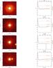 |
Fig. B.2 Detection limits in the H band. |
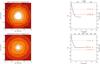 |
Fig. B.2 continued. |
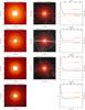 |
Fig. B.3 Detection limits in the J band. |
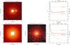 |
Fig. B.3 continued. |
Appendix C: The HD 49095 triple system
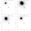 |
Fig. C.1 Orbit of the binary companion to HD 49095 resolved over 3.5 yr. The blue and red dots mark the positions of CC1 and CC2, respectively, as retrieved by the deconvolution algorithm. The axes give the projected separations with respect to CC1. |
Appendix D: HD 32743 motion over 49 years
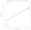 |
Fig. D.1 Motion of HD 32743 (η1 Pic) CC1 on the sky considering the 1946 archive values for ρ and θ in the CCDM with arbitrary uncertainties. The filled red dot indicates the position measured in 2005. This companion candidate is considered as a probable background object. |
The excess of scatter in radial velocity measurements resulting from inhomogeneities on the stellar surface and stellar envelope pulsations.
Velocimetric detection limits for stars earlier than B8 does not fall into the planet domain.
Here, we assume that the binary has the same age as the primary (~5 Gyr), hence on the main sequence.
In the case of HD 41742, there is a 4th companion lying out of the field of view of this survey.
Acknowledgments
We are grateful to the referee, J. Carson, for having promptly provided a useful report on this work. These results have extensively made use of the SIMBAD and VizieR databases, operated at the CDS, Strasbourg, France. This publication makes use of data products from the Two Micron All Sky Survey, which is a joint project of the University of Massachusetts and the Infrared Processing and Analysis Center/California Institute of Technology, funded by the National Aeronautics and Space Administration and the National Science Foundation. This research has made use of the Washington Double Star Catalogue maintained at the US Naval Observatory. AML, DE, and GC acknowledge financial support from the French National Research Agency (ANR contract NT05-44463). DE also acknowledges support from the Centre National d’Études Spatiales (CNES). vspace*-1.5mm
References
- Baraffe, I., Chabrier, G., Allard, F., & Hauschildt, P. H. 1998, A&A, 337, 403 [NASA ADS] [Google Scholar]
- Bevington, P. R., & Robinson, K. D. 2003, Data Reduction and Error Analysis for the Physical Sciences (Boston: McGraw-Hill), 3rd edn. [Google Scholar]
- Boccaletti, A., Chauvin, G., Baudoz, P., & Beuzit, J.-L. 2007, A&A, 482, 939 [Google Scholar]
- Bonfils, X., Mayor, M., & Delfosse, X., et al. 2007, A&A, 474, 293 [NASA ADS] [CrossRef] [EDP Sciences] [Google Scholar]
- Boss, A. P. 1997, Science, 276, 1836 [NASA ADS] [CrossRef] [Google Scholar]
- Boss, A. P. 2006, ApJ, 643, 501 [NASA ADS] [CrossRef] [Google Scholar]
- Bouchy, F., Hébrard, G., Udry, S., et al. 2009, A&A, 505, 853 [NASA ADS] [CrossRef] [EDP Sciences] [Google Scholar]
- Chauvin, G., Lagrange, A.-M., Dumas, C., et al. 2004, A&A, 425, L29 [NASA ADS] [CrossRef] [EDP Sciences] [MathSciNet] [Google Scholar]
- Chauvin, G., Lagrange, A.-M., Dumas, C., et al. 2005a, A&A, 438, L25 [NASA ADS] [CrossRef] [EDP Sciences] [Google Scholar]
- Chauvin, G., Lagrange, A.-M., Lacombe, F., et al. 2005b, A&A, 430, 1027 [NASA ADS] [CrossRef] [EDP Sciences] [Google Scholar]
- Chauvin, G., Lagrange, A.-M., Zuckerman, B., et al. 2005c, A&A, 438, L29 [NASA ADS] [CrossRef] [EDP Sciences] [Google Scholar]
- Chauvin, G., Lagrange, A.-M., Udry, S., et al. 2006, A&A, 456, 1165 [NASA ADS] [CrossRef] [EDP Sciences] [MathSciNet] [Google Scholar]
- Chauvin, G., Lagrange, A.-M., Bonavita, M., et al. 2010, A&A, 509, A52 [NASA ADS] [CrossRef] [EDP Sciences] [Google Scholar]
- Cox, A. N. 2000, Allen’s Astrophysical Quantities (New York: AIP Press; Springer), 4th edn. [Google Scholar]
- Crida, A., Masset, F., & Morbidelli, A. 2009, ApJ, 705, L148 [NASA ADS] [CrossRef] [Google Scholar]
- Devillard, N. 1997, The Messenger, 87, 19 [NASA ADS] [Google Scholar]
- Desidera, S., & Barbieri, M. 2007, A&A, 462, 345 [NASA ADS] [CrossRef] [EDP Sciences] [Google Scholar]
- Desort, M., Lagrange, A.-M., Galland, F., et al. 2008, A&A, 491, 883 [NASA ADS] [CrossRef] [EDP Sciences] [Google Scholar]
- Dodson-Robinson, S. E., Veras, D., Ford, E. B., & Beichman, C. A. 2009, ApJ, 707, 79 [NASA ADS] [CrossRef] [Google Scholar]
- Doyon, R., Nadeau, D., Vallée, P., et al. 1998, SPIE, 3354, 760 [Google Scholar]
- Ducati, J. R., Bevilacqua, C. M., Rembold, S. B., & Daiana, R. 2001, ApJ, 558, 309 [NASA ADS] [CrossRef] [Google Scholar]
- Duchêne, G., McCabe, C., Pinte, C., et al. 2010, ApJ, 709, L114 [NASA ADS] [CrossRef] [Google Scholar]
- Eggen, O. J. 1991a, AJ, 102, 1826 [NASA ADS] [CrossRef] [Google Scholar]
- Eggen, O. J. 1991b, AJ, 102, 2028 [NASA ADS] [CrossRef] [Google Scholar]
- Eggen, O. J. 1998, AJ, 116, 284 [NASA ADS] [CrossRef] [Google Scholar]
- Eggenberger, A., Udry, S., & Mayor, M. 2004, A&A, 417, 353 [NASA ADS] [CrossRef] [EDP Sciences] [Google Scholar]
- Eggenberger, A., Udry, S., Chauvin, G., et al. 2007, A&A, 474, 273 [NASA ADS] [CrossRef] [EDP Sciences] [Google Scholar]
- Frankowski, A., Jancart, S., & Jorissen, A. 2007, A&A, 464, 377 [NASA ADS] [CrossRef] [EDP Sciences] [Google Scholar]
- Gray, R. O., Corbally, C. J., Garrison, R. F., et al. 2006, AJ, 132, 161 [NASA ADS] [CrossRef] [Google Scholar]
- Grosbøl, P. J. 1978, A&AS, 32, 409 [Google Scholar]
- Goldin, A., & Makarov, V. V. 2007, ApJS, 173, 137 [NASA ADS] [CrossRef] [Google Scholar]
- Hauck, B. 1986, A&A, 155, 371 [NASA ADS] [Google Scholar]
- Hinkley, S., Oppenheimer, B. R., Brenner, D., et al. 2010, ApJ, 712, 421 [NASA ADS] [CrossRef] [Google Scholar]
- Hubrig, S., Le Mignant, D., North, P., & Krautter, J. 2001, A&A, 372, 152 [NASA ADS] [CrossRef] [EDP Sciences] [Google Scholar]
- Holmberg, J., Nordström, B., & Andersen, J. 2009, A&A, 501, 941 [NASA ADS] [CrossRef] [EDP Sciences] [Google Scholar]
- Huang, W., & Gies, D. R. 2008, ApJ, 683, 1045 [NASA ADS] [CrossRef] [Google Scholar]
- Ida, S., & Lin, D. N. C. 2004, ApJ, 616, 567 [NASA ADS] [CrossRef] [MathSciNet] [Google Scholar]
- Ida, S., & Lin, D. N. C. 2005, ApJ, 626, 1045 [NASA ADS] [CrossRef] [Google Scholar]
- Kalas, P., Graham, J. R., Chiang, E., et al. 2008, Science, 322, 1345 [NASA ADS] [CrossRef] [PubMed] [Google Scholar]
- Kennedy, G. M., & Kenyon, S. J. 2007, Ap&SS, 311, 9 [NASA ADS] [CrossRef] [Google Scholar]
- King, J. R., Villarreal, A. R., Soderblom, D. R., Gulliver, A. F., & Adelman, S. J. 2003, AJ, 125, 1980 [NASA ADS] [CrossRef] [Google Scholar]
- Kratter, K. M., Murray-Clay, R. A., & Youdin, A. N. 2010, ApJ, 710, 1375 [NASA ADS] [CrossRef] [Google Scholar]
- Lagrange, A.-M., Desort, M., Galland, F., Udry, S., & Mayor, M. 2009a, A&A, 495, 335 [NASA ADS] [CrossRef] [EDP Sciences] [Google Scholar]
- Lagrange, A.-M., Gratadour, D., Chauvin, G., et al. 2009b, A&A, 493, L21 [NASA ADS] [CrossRef] [EDP Sciences] [Google Scholar]
- Lagrange, A.-M., Kasper, M.Boccaletti, A., et al. 2009c, A&A, 506, 927 [NASA ADS] [CrossRef] [EDP Sciences] [Google Scholar]
- Lagrange, A.-M., Bonnefoy, M., Chauvin, G., et al. 2010, Science, 329, 57 [NASA ADS] [CrossRef] [PubMed] [Google Scholar]
- Laughlin, G., Bodenheimer, P., & Adams, F. C. 2004, ApJ, 612, L73 [NASA ADS] [CrossRef] [Google Scholar]
- Lenzen, R., Hartung, M., Brandner, W., et al. 2003, SPIE, 4841, 944 [Google Scholar]
- Lodato, G., Delgado-Donate, E., & Clarke, C. J. 2005, MNRAS, 364, L91 [NASA ADS] [CrossRef] [Google Scholar]
- Lovis, C., & Mayor, M. 2007, A&A, 472, 657 [NASA ADS] [CrossRef] [EDP Sciences] [Google Scholar]
- Lowrance, P. J., McCarthy, C,Becklin, E. E., et al. 1999, ApJ, 512, L69 [NASA ADS] [CrossRef] [Google Scholar]
- Lowrance, P. J., Schneider, G., Kirkpatrick, J. D., et al. 2000, ApJ, 541, 390 [NASA ADS] [CrossRef] [Google Scholar]
- Luhman, K. L., & Jayawardhana, R. 2002, ApJ, 566, 1132 [NASA ADS] [CrossRef] [Google Scholar]
- Mannings, V., & Barlow, M. J. 1998, ApJ, 497, 330 [NASA ADS] [CrossRef] [Google Scholar]
- Marois, C., Macintosh, B., Barman, T., et al. 2008, Science, 322, 1348 [NASA ADS] [CrossRef] [PubMed] [Google Scholar]
- McCaughrean, M. J., & Stauffer, J. R. 1994, AJ, 108, 1382 [NASA ADS] [CrossRef] [Google Scholar]
- Morales, F. Y., Werner, M. W., Bryden, G., et al. 2009, ApJ, 699, 1067 [NASA ADS] [CrossRef] [Google Scholar]
- Mordasini, C., Alibert, Y., Benz, W., & Naef, D. 2009, A&A, 501, 1161 [NASA ADS] [CrossRef] [EDP Sciences] [Google Scholar]
- Mugrauer, M., Seifahrt, A., & Neuhäuser, R. 2007, MNRAS, 378, 1328 [NASA ADS] [CrossRef] [Google Scholar]
- Neuhäuser, R., Günther, E. W., Alves, J., et al. 2003, AN, 324, 535 [Google Scholar]
- Makarov, V. V. 2007, ApJS, 169, 105 [NASA ADS] [CrossRef] [MathSciNet] [Google Scholar]
- Makarov, V. V., & Kaplan, G. H. 2005, AJ, 129, 2420 [NASA ADS] [CrossRef] [Google Scholar]
- Mayer, L., Wadsley, J., Quinn, T., & Stadel, J. 2005, MNRAS, 363, 641 [NASA ADS] [Google Scholar]
- Mayor, M., Bonfils, X., Forveille, T., et al. 2009a, A&A, 507, 487 [NASA ADS] [CrossRef] [EDP Sciences] [Google Scholar]
- Mayor, M., Udry, S., Lovis, C., et al. 2009b, A&A, 493, 639 [NASA ADS] [CrossRef] [EDP Sciences] [Google Scholar]
- Moshir, M. 1989, Explanatory supplement to the IRAS Faint Source Survey, Infrared Processing and Analysis Center, Pasadena, CA, USA [Google Scholar]
- Nakajima, T., Oppenheimer, B. R., Kulkarni, S. R., et al. 1995, Nature, 378, 463 [NASA ADS] [CrossRef] [Google Scholar]
- Patience, J., White, R. J., Ghez, A. M., et al. 2002, ApJ, 581, 654 [NASA ADS] [CrossRef] [Google Scholar]
- Pollack, J. B., Hubickyj, O., Bodenheimer, P., et al. 1996, Icarus, 124, 62 [NASA ADS] [CrossRef] [Google Scholar]
- Pourbaix, D., Tokovinin, A. A., Batten, A. H., et al. 2004, A&A, 424, 727 [NASA ADS] [CrossRef] [EDP Sciences] [Google Scholar]
- Plavchan, P., Werner, M. W., Chen, C. H., et al. 2009, A&A, 698, 1068 [Google Scholar]
- Rafikov, R. R. 2005, ApJ, 621, L69 [NASA ADS] [CrossRef] [Google Scholar]
- Rieke, G. H., Su, K. Y. L., Stansberry, J. A., et al. 2005, ApJ, 620, 1010 [NASA ADS] [CrossRef] [Google Scholar]
- Rigaut, F., Salmon, D., Arsenault, R., et al. 1998, PASP, 110, 152 [Google Scholar]
- Rivera, E. J., & Lissauer, J. J. 2000, ApJ, 530, 454 [NASA ADS] [CrossRef] [Google Scholar]
- Rousset, G., Lacombe, F., Puget, P., et al. 2003, SPIE, 4839, 140 [Google Scholar]
- Santos, N. C., Israelian, G., & Mayor, M. 2001, A&A, 373, 1019 [NASA ADS] [CrossRef] [EDP Sciences] [Google Scholar]
- Santos, N. C., Israelian, G., & Mayor, M. 2004, A&A, 415, 1153 [NASA ADS] [CrossRef] [EDP Sciences] [Google Scholar]
- Su, K. Y. L., Rieke, G. H., Stansberry, J. A., et al. 2006, ApJ, 653, 675 [NASA ADS] [CrossRef] [Google Scholar]
- Suchkov, A. A., Makarov, V. V., & Voges, W. 2003, ApJ, 595, 1206 [NASA ADS] [CrossRef] [Google Scholar]
- Sumi, T., Bennett, D. P., Bond, I. A., et al. 2010, ApJ, 710, 1641 [NASA ADS] [CrossRef] [Google Scholar]
- Torres, G. 1986, A&AS, 64, 105 [Google Scholar]
- Tokovinin, A. A. 1997, A&AS, 124, 75 [NASA ADS] [CrossRef] [EDP Sciences] [Google Scholar]
- Véran, J.-P. 1997, Ph.D. Thesis, École Nationale Supérieure des Télécommunications, France [Google Scholar]
- Zucker, S., & Mazeh, T. 2002, ApJ, 568, L113 [NASA ADS] [CrossRef] [Google Scholar]
- Zuckerman, B., Song, I., & Webb, R. A. 2001, ApJ, 559, 388 [NASA ADS] [CrossRef] [Google Scholar]
All Tables
Multi-epoch measurement results for 41 companion candidates detected around 23 stars of the sample.
All Figures
|
Fig. 1 Colours of stars in the imaging sample. Stars with spectral types F, A, and B are represented as red-, green-, and blue-filled circles, respectively. |
| In the text | |
|
Fig. 2 Spectral types of the stars in the sample. |
| In the text | |
|
Fig. 3 Number of stars per 5-pc distance bin. The F, A, and B stars are represented by the histograms filled with tight diagonal red stripes, diagonal green stripes, and horizontal blue stripes, respectively. The dotted line stands for the whole star sample. |
| In the text | |
|
Fig. 4 Examples of the status determination of companion candidates around HD 14943 (left) and η Tuc (HD 224392; right), from astrometric measurements at two different epochs. The positions on the sky are reported in the upper panel: the candidates were first imaged on 2005-11-07 (filled black circles), then on 2008-08-20 (filled red and blue circles; there are two measurements in the case of HD 14943). The positions predicted for the candidates on 2008-08-20 if they were background objects from the field are indicated by the empty red and blue circles, and their trajectories between the two epochs figured by the black curves, which take the stellar proper motions and the parallactic motions into account. The middle and lower panels show the evolutions of the projected separations and the position angles, respectively, with time. One-sigma error bars are represented. A zero or near-zero evolution of the separation and position angle with time indicates a physical association. The candidate at the left is bound to its star with indicative probabilities Pbkg = 0% and Pcmv = 96.7% (following the calculations of Sect. 4.2), while the candidate at the right is a background contaminant, with Pbkg = 12.0% and Pcmv = 0%. |
| In the text | |
|
Fig. 5 Example of 6-σ detection limits reached for a K = 4.7 mag A0V star at 52.7 pc (HD 2834) using direct imaging (left panel) and coronagraphy (middle panel). Detection limits for the direct and coronagraphic image are given in 2 × 2 and 6 × 6 arcsec2 fields around the star, respectively. The hatched area on the coronagraphic image represents the occulting mask with a diameter of 0″̣7. Classic 1-dimensional 6-σ detection limits (right panel) are extracted from the direct image detection limit map (plain line) and the coronagraphy detection limit map (dotted line) as explained in Sect. 4.3. Mass limits (red lines) are obtained by interpolating Baraffe et al.’s (1998) evolutionary model for a given stellar age (here, 700 Myr). |
| In the text | |
|
Fig. 6 Same as Fig. 5 for a K = 4.3 mag F7V star at 24.6 pc, and an age estimated to ~4.1 Gyr (HD 91889). |
| In the text | |
|
Fig. 7 Median 6-σ detection limits in the
Ks band for F- (red), A- (green), and B-type (blue)
stars, in direct imaging (plain lines) and coronagraphic (dashed lines) modes. The
coronagraphic detection limits are better than the direct imaging ones from 2″ on,
for the reasons given in Sect. 4.3. The
measured separations ρ and magnitude differences
ΔKs of companion candidates confirmed through
multi-epoch observations and those with an undefined status are indicated by
filled and empty circles, respectively. The confirmed companion candidate to
ι Crt, which was only observed in the H band,
is marked by the red square assuming a (H−K)
colour close to 0. The dash-dotted line at |
| In the text | |
|
Fig. 8 Absolute magnitudes vs. projected separations. The legend is the same as for Fig. 7. The absolute magnitudes MKs and projected separations are calculated for each object given its apparent magnitude mKs in the Ks band and distance d from Earth. The 6-σ detection limits shown for F- (red), A- (green), and B-type (blue) stars in direct imaging (plain lines) and coronagraphic (dashed lines) modes are the medians of the detection limits MKs = f(ρ(d),d,mKs) calculated for all stars of a given spectral type. |
| In the text | |
|
Fig. 9 Stars with companion candidates confirmed through multi-epoch observations. North is up and east to the left. Counts on the detector are displayed with a logarithmic scale. |
| In the text | |
|
Fig. 10 The F6.5V star HD 49095 and its binary comoving companion composed of CC1 (blue circle) and CC2 (red circle). The axes are labelled in projected separation with respect to the primary star centroid position (white star). The positions of objects on this image are retrieved using the deconvolution algorithm described in Sect. 4.1. |
| In the text | |
|
Fig. 11 Motion of the binary companion CC2 of HD 49095 (zoom from Fig. 10) relative to CC1 (blue point) between 4 different epochs covering 3.5 yr. The best-fit circular and face-on orbit is depicted, with a semi-major axis of 2.27 AU. |
| In the text | |
|
Fig. 12 Number of detected companions as a function of the projected separation to the primary, per bin of 100 AU. Companions around F stars (red stripes) and A+B stars (green stripes) are differenciated. The black dotted line represents the total number of companions. (a) Confirmed companions only. (b) Confirmed and unconfirmed companions. |
| In the text | |
|
Fig. A.1 Motions of companion candidates measured on the sky relatively to their respective primary stars (at (Δα,Δδ) = (0,0)). The theoretical motion of an object is calculated from its initial first epoch measurement (black filled circle) assuming it is a background contaminant and given the proper and parallactic motions of the primary star (black curve), for the different epochs where measurements have been recorded (empty circles). The measured positions for these different epochs are reported (filled circles) for comparison. When the measurements (filled circles) agree with the theoretical motion path, the companion candidate is likely a background contaminant. |
| In the text | |
|
Fig. A.1 continued. |
| In the text | |
|
Fig. A.1 continued. |
| In the text | |
|
Fig. A.1 continued. |
| In the text | |
|
Fig. A.1 continued. |
| In the text | |
|
Fig. B.1 Detection limits in the Ks band. |
| In the text | |
|
Fig. B.1 continued. |
| In the text | |
|
Fig. B.1 continued. |
| In the text | |
|
Fig. B.1 continued. |
| In the text | |
|
Fig. B.1 continued. |
| In the text | |
|
Fig. B.1 continued. |
| In the text | |
|
Fig. B.1 continued. |
| In the text | |
|
Fig. B.1 continued. |
| In the text | |
|
Fig. B.1 continued. |
| In the text | |
|
Fig. B.1 continued. |
| In the text | |
|
Fig. B.2 Detection limits in the H band. |
| In the text | |
|
Fig. B.2 continued. |
| In the text | |
|
Fig. B.3 Detection limits in the J band. |
| In the text | |
|
Fig. B.3 continued. |
| In the text | |
|
Fig. C.1 Orbit of the binary companion to HD 49095 resolved over 3.5 yr. The blue and red dots mark the positions of CC1 and CC2, respectively, as retrieved by the deconvolution algorithm. The axes give the projected separations with respect to CC1. |
| In the text | |
|
Fig. D.1 Motion of HD 32743 (η1 Pic) CC1 on the sky considering the 1946 archive values for ρ and θ in the CCDM with arbitrary uncertainties. The filled red dot indicates the position measured in 2005. This companion candidate is considered as a probable background object. |
| In the text | |
Current usage metrics show cumulative count of Article Views (full-text article views including HTML views, PDF and ePub downloads, according to the available data) and Abstracts Views on Vision4Press platform.
Data correspond to usage on the plateform after 2015. The current usage metrics is available 48-96 hours after online publication and is updated daily on week days.
Initial download of the metrics may take a while.