| Issue |
A&A
Volume 523, November-December 2010
|
|
|---|---|---|
| Article Number | A91 | |
| Number of page(s) | 12 | |
| Section | Planets and planetary systems | |
| DOI | https://doi.org/10.1051/0004-6361/201014708 | |
| Published online | 18 November 2010 | |
Stellar characterization of CoRoT/Exoplanet fields with MATISSE ⋆,⋆⋆
1
Laboratoire d’Astrophysique de Marseille (UMR 6110), OAMP, Université
Aix-Marseille & CNRS,
38 rue Frédéric Joliot Curie,
13388
Marseille Cedex 13,
France
e-mail: This email address is being protected from spambots. You need JavaScript enabled to view it.
2
Université Nice Sophia Antipolis, CNRS (UMR 6202), Observatoire de
la Côte d’Azur, Laboratoire Cassiopée, BP 4229, 06304
Nice,
France
3
Institut d’Astrophysique de Paris (UMR7095) CNRS, Université
Pierre & Marie Curie, 98bis Bd Arago, 75014
Paris,
France
4
Observatoire de Haute-Provence, CNRS/OAMP,
04870 St Michel
l’ Observatoire,
France
5
Thüringer Landessternwarte Tautenburg, Sternwarte 5,
07778
Tautenburg,
Germany
6
Research and Scientific Support Department,
European Space Agency (ESA-ESTEC),
PO Box 299, 2200
AG
Noordwijk, The
Netherlands
Received:
1
April
2010
Accepted:
8
July
2010
Abstract
Aims. The homogeneous spectroscopic determination of the stellar parameters is a mandatory step for transit detections from space. Knowledge of which population the planet hosting stars belong to places constraints on the formation and evolution of exoplanetary systems.
Methods. We used the FLAMES/GIRAFFE multi-fiber instrument at ESO to spectroscopically observe samples of stars in three CoRoT/Exoplanet fields, namely the LRa01, LRc01, and SRc01 fields, and characterize their stellar populations. We present accurate atmospheric parameters, Teff, log g, [M/H], and [α/Fe] derived for 1 227 stars in these fields using the MATISSE algorithm. The latter is based on the spectral synthesis methodology and automatically provides stellar parameters for large samples of observed spectra. We trained and applied this algorithm to FLAMES observations covering the Mg i b spectral range. It was calibrated on reference stars and tested on spectroscopic samples from other studies in the literature. The barycentric radial velocities and an estimate of the V sin i values were measured using cross-correlation techniques.
Results. We corrected our samples in the LRc01 and LRa01 CoRoT fields for selection effects to characterize their FGK dwarf stars population, and compiled the first unbiased reference sample for the in-depth study of planet metallicity relationship in these CoRoT fields. We conclude that the FGK dwarf population in these fields mainly exhibit solar metallicity. We show that for transiting planet finding missions, the probability of finding planets as a function of metallicity could explain the number of planets found in the LRa01 and LRc01 CoRoT fields. This study demonstrates the potential of multi-fiber observations combined with an automated classifier such as MATISSE for massive star spectral classification.
Key words: techniques: spectroscopic / stars: fundamental parameters / planetary systems / stars: general
Based on observations collected with the GIRAFFE and UVES/FLAMES spectrographs at the VLT/UT2 Kueyen telescope (Paranal observatory, ESO, Chile: programs 074.C-0633A & 081.C-0413A).
Full Tables 4, 9–11, and 13 are only available in electronic form at the CDS via anonymous ftp to cdsarc.u-strasbg.fr (130.79.128.5) or via http://cdsweb.u-strasbg.fr/cgi-bin/qcat?J/A+A/523/A91
© ESO, 2010
1. Introduction
Since the discovery of the first exoplanet by Mayor & Queloz (1995), large-scale spectroscopic surveys for finding planets have gathered thousands of high resolution spectra. Atmospheric parameters and chemical composition for these samples were determined by Valenti & Fischer (2005) or Sousa et al. (2008). They explored the links between the hosting stars and field stars parameters. This requires a good characterization of the fields in which planets are searched for. The CoRoT (Convection Rotation and Transits, see Baglin et al. 2006 for full details) space mission has obtained light curves with very high relative photometric precision for more than 120000 stars. However, an accurate knowledge of the fundamental parameters of the stars observed by the satellite is mandatory to fully exploit this photometric database.
We performed a first-order spectral classification of the stars in some of the CoRoT/Exoplanet fields using broad-band photometry obtained at the INT/La Palma. The coordinates and magnitudes as well as these photometric spectral types and luminosity classes of the CoRoT stars are available from Exo-Dat (Deleuil et al. 2009; Meunier et al. 2007) and used for the target selection and the precise placement of its photometric masks. However, this spectral classification presents some uncertainties, e.g., the unknown star’s reddening, chemical abundances, and potential binarity. Combining this photometry with intermediate resolution spectroscopy would help in the determination of the physical parameters of the stars.
In this context, we present a fully automated and homogeneous determination of atmospheric parameters from intermediate resolution spectra obtained with the FLAMES/GIRAFFE multi-object facility. This work is the second scientific objective of the study presented by Loeillet et al. (2008), hereafter L08. In that paper, the authors demonstrated the capability of multi-fiber instruments to find planetary candidates by radial velocity techniques. We extended this study by observing a new sample of stars with the same configuration in May–June 2008, to perform a homogeneous spectral characterization of the fields observed by CoRoT. For that purpose, we adapted an algorithm originally developed for the spectroscopic analysis of data to be obtained with the Radial Velocity Spectrometer of the Gaia mission: MATrix Inversion for Spectral SynthEsis, MATISSE (Recio-Blanco et al. 2006; Bijaoui et al. 2008). We measured the effective temperature (Teff), the surface gravity (log g), the overall metallicity ([M/H]), and the α-enhancement ([α/Fe]) of 1227 stars, the barycentric radial velocity of 1534 stars, and estimated the projected rotational velocity (V sin i) of 1604 stars located in the LRa01, LRc01, and SRc01 fields. The whole data set, observational set-ut and date, and the derived physical parameters are available to the community through the CoRoT database, Exo-Dat1. We applied the relation linking the probability of finding planets with the metallicity of the host stars (Udry & Santos 2007) to the de-biased sample.
The structure of this paper is as follows. Section 2 describes the observations, the instrument setup, and the target selection. Section 3 continues with data reduction and processing. The automatic algorithm, its implementation, and limitations are developed in Sect. 4. The results and a discussion can be found in Sects. 5 and 6, respectively.
2. Observations
In January 2005 and May–June 2008, we obtained 13 half-nights in visitor mode to perform spectroscopic observations with the FLAMES multi-object facility coupled with the GIRAFFE and UVES spectrographs (programs 074.C-0633A and 081.C- 0413A). The instrument is mounted on the 8.2 m Kueyen telescope (UT2) based at the ESO-VLT.
The FLAMES/GIRAFFE observations were performed in the MEDUSA configuration, using the HR9B spectral domain. This setup covers about 200 Å centered at 5258 Å around the Mg i b lines, with an intermediate resolving power (R = 25900) and a CCD pixel sampling of 0.05 Å. This instrumental configuration was selected in 2005 for it contains many thin spectral lines leading to a good radial velocity accuracy (Royer et al. 2002). This wavelength range is also interesting for the determination of spectroscopic parameters since it contains many metallic lines that can constrain the temperature and metallicity, and some ionized spectral lines that can help to constrain the surface gravity. As a part of the radial velocity follow-up of CoRoT exoplanet candidates, we observed 7 additional stars, at a higher spectral resolution and across a wider wavelength range with the UVES/FLAMES facility. We used the red arm of the spectrograph at a central wavelength of 5800 Å, covering about 2000 Å with a resolving power of about 47000.
The 2005 campaign was dedicated to the radial velocity follow-up of selected CoRoT stars in the so-called anticenter direction field (LRa01: Long Run Anticenter 01), at Galactic coordinates l ≃ 212.2°, b ≃ − 1.9°. Full description of the target selection and observational strategy for this first campaign can be found in Sect. 2 of L08. The targets observed during the 2008 campaign belong to the SRc01 (Short Run Center 01; l ≃ 36.8°, b ≃ − 1.2°) and LRc01 (Long Run Center 01; l ≃ 37.7°, b ≃ − 7.5°) CoRoT fields, close to the Galactic center direction. The observation strategy for the 2008 campaign was slightly different from the 2005 one since the main purpose of the GIRAFFE observations was to characterize the stellar population observed by CoRoT, which was only a secondary objective for the 2005 campaign.
Priority criteria. 9 is the highest priority, 1 the lowest.
For the 2008 campaign, each observed field was centered around the CoRoT planetary candidates observed with UVES. The FLAMES/GIRAFFE fiber allocation was performed taking into account the instrumental constraints (magnitude limits, fiber positions, etc.) and according to four different levels of priorities, as described in Table 1. Using the spectral classification available in Exo-Dat, we gave the highest priority to solar-type dwarf and sub-giant stars since these were the stellar populations we wished to characterize. High priorities were assigned to bright targets to ensure good signal-to-noise ratios (SNRs) in short exposure times. About 4–5 fibers were used to register the sky signal. These selection criteria were chosen to be very similar to the 2005 ones to ensure the homogeneity of the whole sample. Bad weather conditions and instrumental issues affected the second observing campaign. Out of the 20 planned configurations, we managed to observe only 10 FLAMES fields, as listed in the journal of the observations reported in Table 2.
In total, we obtained 1241 spectra of stars located in the SRc01 and LRc01 CoRoT fields. These new spectra were analyzed together with the 772 spectra of LRa01 stars. Hereafter, we call the pointing direction related to the LRc01 and SRc01 fields center and related to the LRa01 field anticenter.
Journal of the 2008 observations with the coordinates of the field centers and the adopted exposure time.
3. Data processing
The 2005 frames were reduced using the GIRAFFE BaseLine Data Reduction Software (girbldrs v1.12, see Royer et al. 2002; Blecha et al. 2000). The second epoch data were reduced using the standard ESO reduction pipeline for GIRAFFE spectra (version 6.2.a2). Both pipelines apply the standard reduction processes of bias and dark subtraction, and scattered light correction.
The spectra from the 2005 campaign were extracted with the optimum method. Those from the 2008 campaign were extracted using the standard method. According to the standard extraction, for each localized fiber, the spectra are extracted by summing the flux of the pixels along the direction perpendicular to the dispersion axis. The optimum extraction method uses the shape of the fiber profile to weight the flux as a function of noise (Horne 1986). The use of optimal extraction for the second epoch data did not show a sufficient improvement to justify its use.
For the 2005 spectra, the wavelength solution was calculated once at the beginning of the campaign and used for the whole data-set. Instrumental drift was followed during the run with simultaneous Th-Ar lamps. For the second epoch data, the wavelength calibration was performed using non-simultaneous Th-Ar spectra since we did not require as high a precision in radial velocity as L08. A sky correction was finally applied to each stellar spectrum using standard IRAF routines.
Combining the two campaigns, the sample of GIRAFFE data contains spectra for 1914 different CoRoT targets with a SNR ratio ranging from 10 to 100. The analysis of such a large amount of spectra requires a completely automated and homogeneous processing of the whole sample. To render every spectrum comparable to a reference library, we applied the following procedure.
The raw images contained a significant number of grazing cosmic rays contaminating the dispersion axis. Some spectra were polluted by these high values spikes. We corrected the data for their presence using a sigma clipping technique adjusted to the wavelength domain. This cleaning is a mandatory step to avoid numerical problems during the spectroscopic analysis.
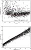 |
Fig. 1 Top: Calibration of the minimal broadening of the CCF measured as a function of the (B − V) color index for slow rotators (V sin i < 20 km s-1). Bottom: Correlation between the V sin i and the FWHM of the CCF for fast rotators. |
We measured the barycentric radial velocity of the stars using a weighted cross-correlation
of each spectrum with a numerical mask. The latter was constructed by Baranne et al. (1996), who identified in the solar spectrum the spectral
lines relevant to radial velocity measurements. The resulting cross-correlation function
(CCF) is fitted by a Gaussian function. As recalled by L08, it provides the barycentric radial velocity
(Vrad) and an estimate of the projected rotational velocity
(V sin i). Following Santos et al. (2002) methodology, we calibrated the relation between the
V sin i and the broadening of the CCF
(σ), for the FLAMES/GIRAFFE instrument
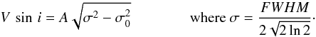 (1)For the slow rotators with typical
V sin i < 20 km s-1, we
found the coefficient A = 1.8 ± 0.1 by adjusting the slope of Eq. (1) with
synthetic stellar spectra. The minimal broadening σ0 in Eq. (1)
as a function of the (B − V) color index (see Fig. 1, upper panel) was fitted by the relation
(1)For the slow rotators with typical
V sin i < 20 km s-1, we
found the coefficient A = 1.8 ± 0.1 by adjusting the slope of Eq. (1) with
synthetic stellar spectra. The minimal broadening σ0 in Eq. (1)
as a function of the (B − V) color index (see Fig. 1, upper panel) was fitted by the relation
 (2)with the B and
V retrieved from Exo-Dat. For faster rotators
(V sin i > 20 km s-1),
the previous relation is no longer valid. We convolved a set of 10000 interpolated synthetic
spectra with different rotational broadening values ranging from 1.0 to
80.0 km s-1. The fit of the V sin i as a
function of the FWHM, shown in Fig. 1
(lower panel), gives
(2)with the B and
V retrieved from Exo-Dat. For faster rotators
(V sin i > 20 km s-1),
the previous relation is no longer valid. We convolved a set of 10000 interpolated synthetic
spectra with different rotational broadening values ranging from 1.0 to
80.0 km s-1. The fit of the V sin i as a
function of the FWHM, shown in Fig. 1
(lower panel), gives 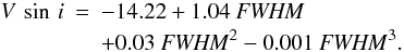 (3)We applied Eq. (1) to the slow rotators
(V sin i < 20 km s-1)
and Eq. (3) to the faster rotators. We checked that the rotational velocity calculated for
stars close to 20 km s-1 gave very close results with both methods.
(3)We applied Eq. (1) to the slow rotators
(V sin i < 20 km s-1)
and Eq. (3) to the faster rotators. We checked that the rotational velocity calculated for
stars close to 20 km s-1 gave very close results with both methods.
The derived radial and projected rotational velocities are listed in Table 9. A quality flag has been added for V sin i, as explained in more detail in Sect. 5 and Table 9. For the SRc01 field, no V magnitudes are available in Exo-Dat. We thus applied only Eq. (3) to derive the V sin i value of the stars in the SRc01 field, as clearly specified in Table 9. Taking into account the limitations of Eq. (3), we preferred to indicate a lower limit of 40 km s-1 when V sin i > 40 km s-1. As described in the following section, we applied MATISSE only to the slower rotators in the sample since our tests showed that the results are not affected by the stellar rotation as long as V sin i is lower than ~11 km s-1.
Each spectrum was then corrected for its Vrad. The same analysis with different masks (F0, K5, M4) showed no significant improvements on the velocity precision, ≃ 0.2 km s-1, and no important mask effect on the final value.
We estimated the position of the pseudo-continuum, that is the apparent continuum. For that purpose, the spectral lines were first removed by an iterative sigma-clipping method. The iterations were stopped when the dispersion of the remaining pixels reached the spectrum noise level. The position of the pseudo-continuum was then found by fitting a low order polynomial. This first order normalized spectrum was then iteratively improved with the results from the MATISSE analysis, as described in Sect. 4.3.
4. Automatic parametrization of stellar spectra with the MATISSE algorithm
The stellar characterization of our sample includes the determination of the following spectroscopic parameters: the effective temperature (Teff), the surface gravity (log g), the overall metallicity ([M/H]), and the α-enhancement ([α/Fe]).
For that purpose, we used the MATISSE (MAtrix Inversion for Spectral SynthEsis) algorithm, described in Recio-Blanco et al. (2006), which is connected to Local MultiLinear Regression methods. The stellar parameters are estimated by projections on relevant functions, B(λ), derived from a multi-linear regression. Since it was initially developed for the Gaia-RVS instrument, it is a very efficient means of analyzing robustly and automatically large samples of stellar spectra. In the present study, we trained MATISSE to the FLAMES instrument and in particular to the HR9B setup.
The algorithm behavior as a function of SNR led us to apply an iterative inversion in the computation of the B(λ) functions during the learning phase of MATISSE (Recio-Blanco et al. 2006; Bijaoui et al. 2008), in the case of too noisy data. In the following, for high SNR theoretical spectra, we consider the results obtained with a direct inversion method. For our observed spectra, we noted that the iterative algorithm provided more reliable results.
The next section describes the grid used for the learning phase of MATISSE. We then describe the procedure and estimate the errors derived by applying MATISSE on the stellar spectra.
4.1. The grid of synthetic spectra
For the training of MATISSE, a grid of theoretical spectra with the same spectral resolution and sampling as our observed data is required. For the computation of this grid, one has to keep in mind that the reliability of the atomic data is crucial when deriving accurate parameters from the stellar spectra. We used a list of atomic lines derived from the Vienna Atomic Line Database (VALD: Kupka et al. 1999) and lists of molecular lines for the species CH, C2, CN, OH, MgH, SiH, CaH, FeH, TiO, VO, and ZrO and their corresponding isotopes (kindly provided by B. Plez – see Recio-Blanco et al. 2006 for a complete description). We calibrated the atomic line-list with observed spectra of the Sun (very high resolution Kurucz solar spectrum) and Arcturus (spectra from Hinkle et al. 2003).
The parameters used for the spectral synthesis of these stars are given in Table 3 and the solar abundances are the same as those indicated by Recio-Blanco et al. (2006). For Arcturus, we used the abundances described in Smith et al. (2000) scaled to our solar model.
Atmospheric parameters used for the synthetic spectra of the stars used for checking the line-list.
For the line-list calibration, we first applied the oscillator strength modifications described in Gustafsson et al. (2008), and checked that these modifications improved our fit of the solar spectrum, at our working spectral resolution and range. We then calibrated the oscillator strengths of about 300 atomic lines at our working resolution, while verifying the coherence with the high resolution solar spectrum. The χ2 between the observed solar spectrum and the theoretical one was improved by a factor two. We also calibrated a few lines in the Arcturus spectrum, checking that it did not degrade the agreement on the solar spectrum. Finally, we checked that all these modifications also fitted the Procyon A spectrum from the UVES Paranal Observatory Project (Bagnulo et al. 2003, and parameters in Table 3). We preferred not to modify any oscillator strengths with this star since Procyon A parameters and furthermore its abundances are not accurately enough known. The modified atomic line data are presented in Table 4. No modification was made to the oscillator strengths of the molecular data.
Shortened list of the modified atomic data.
From this calibrated line-list, we computed a grid of theoretical stellar spectra based on a new generation of MARCS stellar model-atmospheres (Gustafsson et al. 2008) with the turbospectrum code (Alvarez & Plez 1998, and further improvements by Plez). The spectra were calculated assuming a plane-parallel geometry and ξt = 1 km s-1 for stars with log g ≥ 3.5 dex, and a spherical geometry, ξt = 2 km s-1, and a solar mass for star with log g ≤ 3.0 dex. The calculation of the grid followed the same process as described by Recio-Blanco et al. (2006). The final library contains 11 940 spectra and covers the spectral domain from 5141.70 to 5347.15 Å with a sampling of 0.07 Å and a resolving power of 25900. The parameter ranges covered by the grid are presented in Table 5. For stars with [M/H] ≥ + 0.0 dex, we took [α/Fe] = 0.0 dex and for stars with [M/H] ≤ − 1.0 dex, we chose [α/Fe] = 0.4 dex. Between these two metallicities, a linear relation as a function of the metallicity was computed for the [α/Fe] value. The [α/Fe] variations (−0.4, −0.2, 0.0, + 0.2, + 0.4) around this law were then considered for the calculations of the spectra.
Stellar atmospheric parameters of the reference grid used by MATISSE.
To test the validity of our synthetic spectra, we applied the whole procedure to the spectra used for the calibration of the atomic data. It is mandatory to verify that our procedure is self-consistent and that we do not neglect any sources of uncertainty. We ensured that the stellar parameters obtained for these stars are consistent with the values in Table 3. To test this calibration, we also processed the GIRAFFE solar atlas2 in exactly the same way as our FLAMES observations. The mean parameters obtained over the 129 spectra are Teff = 5740 ± 4 K, log g = 4.48 ± 0.01 dex, [M/H] = 0.0 ± 0.004 dex, and [α/Fe] = 0.02 ± 0.002 dex (the error bars coming from the dispersion). These results show the reliability of this calibration and, by extension, of the results obtained in this study. The absolute precision of our procedure was evaluated by performing a series of tests described in the following subsections.
4.2. Relative precision of the parameters
To evaluate the relative precision from one star to the other, we applied MATISSE to a large number (104) of interpolated synthetic spectra with randomly chosen parameters. We added Gaussian noise to these spectra simulating SNR values representative of our sample: 10, 20, 50, and 100. Figure 3 shows the evolution of the error at 70% of the error distribution as a function of the SNR. This error is caused only by the dispersion in the results since the systematic uncertainty is always negligible. These dispersion errors become negligible at SNR > 100. For cool metal-rich stars, which exhibit more spectral lines, more information about the stellar parameters is available, resulting systematically in lower dispersions. The analysis of the cumulative error distribution (Table 6 and Fig. 3) showed that most of the parameters are recovered with a very high accuracy.
 |
Fig. 2 Kinematics results: distribution of the barycentric radial velocities in the two pointing directions (top) and the projected rotational velocities (bottom) for the whole sample. |
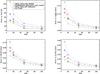 |
Fig. 3 Internal error at 70% of the error distribution as a function of the SNR for cool dwarf metal-rich stars (Teff ≤ 5500 K, log g ≥ 4.0 dex, [M/H] ≥ 0.0 dex, green diamonds), cool giants with intermediate metallicity (Teff ≤ 5500 K, log g ≤ 3.0 dex, 0.0 > [M/H] ≥ − 1.5 dex red stars), hot subgiants metal poor (Teff > 5500 K, 4.0 > log g ≥ 3.5 dex, [M/H] < − 0.75 dex, black crosses), and the whole sample of interpolated spectra (blue triangles). |
Maximum absolute value of the internal error for various proportions of the interpolated spectra at SNR = 10, SNR = 20 and SNR = 50.
4.3. Other sources of uncertainty
We explored the impact on the stellar atmospheric parameters derived by MATISSE of a potential error in the radial velocity, the normalization, and the effect of the rotational velocity.
A large uncertainty in the radial velocity will result in a poor correction of its effects, creating an error in the determination of the various stellar parameters. Several interpolated spectra were shifted by different values of the radial velocity to evaluate these source of errors. We found that, as long as the error in the Vrad remains lower than 1 km s-1(~10% of the resolving power), the final uncertainty in the MATISSE parameters is lower than the internal precision, presented in Sect. 4.2. Since the mean error in the estimated radial velocity for our observed targets is about 200 m s-1, we conclude that this source of uncertainty can be neglected in our study.
The rotation of the star broadens the spectral lines, and can also introduce an error in the stellar parameters. The MATISSE algorithm was trained for non-rotating stars, which represent the vast majority of our sample (see Fig. 2). Using a set of broadened synthetic spectra, we explored the effect of the stellar rotation on the photospheric parameters. We found that the precision of the parameters is smaller than the internal precision when V sin i ≤ 10 km s-1. Stars with higher rotational velocity were disregarded in this study.
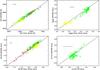 |
Fig. 4 Comparison of the stellar atmospheric parameters derived by MATISSE and those of the literature. Red crosses: Prugniel et al. (2007); green diamond: Allende Prieto et al. (2004); blue circles: UVES spectra & parameters from Prugniel et al. (2007); yellow triangles : Santos et al. (2009). |
Finally, we investigated the influence of the uncertainty on the shape and level of the continuum during the normalization process. For this purpose, we calculated a set of theoretical spectra at a SNR of 20. We modeled a departure from the true continuum by multiplying each of them by a polynomial of the second degree. Each coefficient was fixed at a level of 20% of the error in the position, 10% of the error in the slope, and 10% of the error in the second order shape of the continuum. Feeding these very badly normalized spectra into MATISSE, we found that the errors due to the normalization only are ΔTeff = 175 K, Δlog g = 0.274 dex, Δ[M/H] = 0.388 dex, Δ[α/Fe] = 0.207 dex at most (see Sect. 4.4). This study confirms that the normalization is a matter of prior importance and must be carefully taken into account. We noted that the effect is more important for high SNR spectra for which normalization is a critical issue. To overcome this issue, we implemented supplementary iterations for the placement of the continuum. Each observed spectrum was divided by the synthetic spectrum calculated with the first estimate of the photospheric parameters obtained with MATISSE. The residual of the division was then cleaned from remaining spectral lines and fitted by a low order polynomial. The observed spectrum was divided by this new continuum. A new estimate of the photospheric parameters was made using this re normalized spectrum. A few iterations were sometimes necessary before reaching a stable solution for the atmospheric parameters. This iterative normalization ensures the minimization of this source of uncertainty that can cause large errors in the estimation of the stellar parameters.
4.4. Comparison with libraries of stellar atmospheric parameters
To validate the stellar parameters derived with MATISSE, we retrieved spectra from various libraries: the Elodie 3.1 archive (Prugniel et al. 2007), the S4N study (Allende Prieto et al. 2004), and the Santos et al. (2009) work. We adapted these spectra to our spectral domain and resolution.
The Elodie library contains a quality flag for the Teff, log g, and [Fe/H] taken from the literature. To ensure that the determination of the spectroscopic parameters are of good accuracy, we selected only the stars with high quality criteria for the Teff and the metallicity. These stars presented a poor log g quality criterion, so we decided not to include it in our sample. We also selected 90 stars from the S4N study, the remaining 29 being either fast rotators or stars for which the parameters were not determined in this study. The surface gravity provided in the S4N study was not derived spectroscopically. The spectroscopic method used by these authors showed a too high discrepancy with literature parameters (Allende Prieto et al. 2003). Hence, this parameter was derived by the algorithm described by Allende Prieto et al. (2004) from isochrones tracks and parallaxes from the HIPPARCOS catalogue. For this sample, we therefore compare spectroscopic gravities from MATISSE to evolutionary ones. In the literature, and in particular in Allende Prieto et al. (2004), the metallicity is inferred from the iron content ([Fe/H]). If the star appears not to have peculiar abundances, this value should be equal to the overall metallicity. For the [α/Fe] comparison, we used the abundances for the neutral magnesium, calcium, and silicium, determined by Allende Prieto et al. (2004), since these lines are present in our spectral range. Finally, the study of Santos et al. (2009) was interesting because it includes giant stars. We selected only these stars so as to probe the efficiency of MATISSE for giant targets, uncovered by the two previous studies.
Uncertainty at 70% of the error distribution on the measurement of stellar parameters with spectra from the literature.
In Fig. 4, we compare MATISSE spectroscopic parameters as a function of the literature ones. The parameters derived by MATISSE are available in electronic Tables 10, 11, and 13. We find very good agreement over the four atmospheric parameters: 70% of these stars have difference lower than ~85 K in Teff, ~0.2 dex in log g, ~0.15 dex in [M/H], and ~0.1 dex in [α/Fe] (see Table 7). This shows that for these high SNR observed spectra, the total error on the estimation of the parameters is at least four times higher than for interpolated synthetic spectra (internal error negligible for SNR > 100 – see Sect. 4.2 and Fig. 3). This illustrates that the total error in the estimation of the parameters is caused not only by the method, which exhibits an external source of uncertainty.
We took advantage of multiple observations in our sample to evaluate the real total error on the estimation of every spectroscopic parameter. About fifty stars in the center direction were observed twice and analyzed separately by the entire pipeline. The SNRs of these data range between 5 and 60. The error at 70% of the distribution of the difference between the two determinations provides another estimate of the uncertainty. We combined this uncertainty with the internal error and the external error (quadratic sum) to estimate the total errors of σTeff = 140 K, σlog g = 0.27 dex, σ[M/H] = 0.19 dex, and σ[α/Fe] = 0.09 dex. We recall that for these samples, the relative precision from one star to another is much lower and given in Table 6.
Number of targets according to the kinematics analysis.
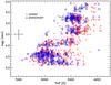 |
Fig. 5 Hertzsprung-Russell diagram with the Teff and log g derived by MATISSE. The red crosses are stars from the LRc01 and the blue triangles from the LRa01 field. |
5. Results
Table 8 reports a brief summary of the numbers of CoRoT stars presented in our study. It lists the number of observed targets, the number of stars for which we derived the physical parameters with MATISSE, the number of detected double-lined spectroscopic binaries (SB2), and the number of stars with estimated radial and projected rotational velocities. For the targets observed in the LRa01, we used the radial velocities as reported in the study performed by L08. Most of the targets presenting no CCF in the center direction were missed due to the poor quality of the input astrometry in the SRc01 field.
The barycentric radial velocities, presented in Table 9, were measured for 77% of the stars in the center direction and 85% stars in the anticenter direction. We only measured precise radial velocities for stars presenting a CCF with a reasonable contrast and not dominated by strong rotational broadening. The V sin i value was measured for 1604 stars in our sample (Table 9), including objects for which Vrad had not been well determined3. As mentioned in Sect. 3, the V sin i estimations have a quality flag, reported as an exponent of the value in Table 9. Its value is set to be 1 if the V sin i estimate is not affected by noise or a second component in the CCF, 2 if the target is a SB2 and the V sin i is related to the main component of the CCF, and 3 if the contrast and shape of the CCF are insufficient to assure a proper estimate of its parameters. As shown in Fig. 2, most of the stars are slow rotators (V sin i < 10 km s-1 for 75%) as expected for late-type field stars (Gray 2008). In both samples, we excluded from the MATISSE analysis the stars exhibiting a CCF with a FWHM greater than 20 km s-1, SB2, and stars for which no accurate radial velocity was measured because of the bad quality of the CCF.
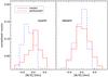 |
Fig. 6 Distribution of the overall metallicity in the two pointing directions for giant (left) and dwarf (right) stars, normalized to the number of stars in each field. |
The MATISSE spectral analysis, described in the previous section, was carried out on a total of 1227 targets that is 65% of the initial number of stars. The results of this analysis are presented in Table 9. Combining the Teff and log g values, we compiled the Hertzsprung-Russell diagram presented in Fig. 5. We observed main-sequence solar-type and cooler giant stars in each of the CoRoT/Exoplanet fields.
Derived physical parameters for the stars observed in the LRa01, LRc01, and SRc01 CoRoT fields.
Derived parameters for the S4N sample from Allende Prieto et al. (2004) (complete table available at the CDS). The first line is the Sun.
Derived parameters for the Elodie3.1 sample from Prugniel et al. (2007) (complete table available at the CDS).
We used the log g derived by MATISSE to differentiate giants, log g < 3.1 dex, and dwarfs, log g > 3.8 dex. This criterion is based on the Straizys & Kuriliene (1981) tables. The metallicity distribution for the giants and dwarfs are presented in Fig. 6. It is similar in the two pointing directions for the dwarfs. For the giants, the maxima of the metallicity distributions are apart one from the other of a few tenth of dex. This could be explained by the radial metallicity gradient generally observed in the Galactic disk (Pedicelli et al. 2009, and references therein).
We compare in Fig. 7 the dwarf-giant dichotomous separation based on the log g derived by MATISSE with the color-magnitude diagram r′ versus (r′ − J). According to this color-magnitude diagram, the stars with an intermediate log g value ([3.1−3.8]) could be considered as giants. We note that the dwarf-giant dichotomy used for this first order classification does not include the uncertainty in the log g. In the following, we include these stars in the giant sample. This figure also shows how the spectroscopic classification easily allows us to distinguish the dwarf and giant populations, this issue being one of the most constraining limitation of the photometric classification, especially for faint targets.
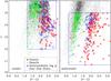 |
Fig. 7 Color magnitude diagrams for the giants (red stars) and the dwarfs (green crosses), as well as the stars with an intermediate log g (blue triangles). All the stars in the Exo-Dat (black dots) are over plotted in the diagram. The dichotomy giant-dwarf comes from the MATISSE parameters. The blue boxes correspond to the limits in color and magnitude for the de-biasing of our sample. |
We find a good agreement between these simple photometric and spectroscopic classifications for the majority of our sample. However, a few stars are misclassified in both pointing directions. In the center field, the outliers could correspond to reddened dwarfs. In the anticenter direction, the obvious misclassification is due to the limits of the grid of the theoretical spectra (see Sect. 4.1). This object is a late-A metal poor star ([M/H] ≃ − 0.7 dex) that exhibits very few lines in the spectral range, resulting in a very difficult classification. We found that ~1% of the stars are misclassified.
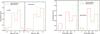 |
Fig. 8 Comparison of the spectral types and luminosity classes derived with MATISSE and with the Exo-Dat photometric classification criteria. |
The photometric classification that is available in Exo-Dat consists of two steps. First, a raw luminosity class was derived from color-magnitude diagrams similar to Fig. 7. Then the final estimates of luminosity classes and spectral types were based on spectral energy distribution (SED) fitting with Pickles (1998) templates. For a full description, we refer to Deleuil et al. (2009). No preliminary classification was available for stars in the SRc01 field, hence the center simply stands for the LRc01 field. In Fig. 8, we compare the results of the spectral analysis performed by MATISSE with the photometric classification available in Exo-Dat. The conversion from Teff-log g to spectral type and luminosity class was performed using the Straizys & Kuriliene (1981) tables. Figure 8 illustrates the reasonable agreement found for the spectral types, whereas the luminosity classes histograms show clearly more dwarfs and less giants than estimated by the photometric classification. A discrepancy was expected between the photometric and spectroscopic luminosity classes since the initial photometric estimation of the luminosity class consisted of a simple cut-off in a color-magnitude diagram, applied to prevent the omission of dwarfs during the CoRoT target selection phase. This cut-off could result in a misidentification of dwarfs and giants. For the faint targets, this becomes a more critical issue since the two populations are mixed (Fig. 7). We indeed found a closer agreeement for the brightest targets in our sample.
6. Discussion
The samples of CoRoT targets for which we determined atmospheric parameters are not representative of the whole fields observed by CoRoT. As described in Sect. 2, we used selection criteria for the multi-fiber observations. As a result, our analysis was focussed primarily on the slowly-rotating population of the FGK stars. To more accurately characterize the stellar population in the exoplanet fields, we took into account the various biases introduced by our selection. We de biased our samples using density plots of the color-magnitude diagrams presented in Fig. 7. The limitations of this study are constrained by the ranges in color and magnitude covered by our observations (blue boxes in Fig. 7). For every bin of 0.5 in r′ and 0.5 in (r′ − J), we randomly selected stars in our observations so as to fill in the two-dimensional distribution in the same proportions as the Exo-Dat one. The number of stars in the two long run fields was large enough to efficiently apply this procedure. This was not the case for the SRc01 field to which we did not apply this de-biasing procedure, so the center field simply stands for the LRc01 field. To validate this procedure, we took advantage of the Besançon Galactic model (Robin et al. 2003). We compared each de-biased field with a simulation taking into account the limits in magnitude and assuming the standard extinction law. We found reasonable agreement for the distributions of Teff and log g.
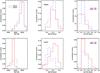 |
Fig. 9 De-biased distributions of the effective temperature, overall metallicity and α-enhancement in the LRc01 (solid red) and LRa01 (dashed blue) fields. The top and lower panels show the distributions for the dwarf and giant stars, respectively. The distributions have been normalized to the number of stars in each field. The percentage given in the [α/Fe] histogram represents the rate of dwarfs (upper panel) and giants (lower panel) in the two fields. |
To compare the two de biased samples, we selected in LRc01 only stars with r′ ≤ 15 mag since this is the magnitude limit of our observations in the LRa01 field. For the two fields, we included the stars with an intermediate log g in the giant sample since they are too few to be analyzed separately and they belong mainly to the giant branch in the color-magnitude diagram (Fig. 7).
Derived parameters for the UVES (POP, Bagnulo et al. 2003) sample and literature from Prugniel et al. (2007).
Derived parameters for the Santos et al. (2009) sample (complete table available at the CDS).
Figure 9 shows the resulting distributions of the Teff, [M/H], and [α/Fe] derived by MATISSE for the two fields normalized to the entire de biased sample. We used the log g values from MATISSE to separate giants from dwarfs as described in the previous section. The dwarf content is roughly similar in the two directions over these three parameters. The majority of these stars are early G or late F stars with solar metallicity. The LRc01 field clearly contains mainly late K giant stars. The other field presents a smoother distribution around K giants, which are slightly hotter. The histograms of [M/H] and [α/Fe] for the giant stars illustrate the metallicity gradient generally observed in our galaxy (Pedicelli et al. 2009), with the center field containing more higher [M/H] giant stars than the anticenter one. For targets with r′ ≤ 15 mag, the two fields can be compared: the LRc01 field is composed of about 41% giant and 59% dwarf stars, whereas the LRa01 field is composed of about 26% giant and 74% dwarf stars. Adding the objects with r′ ≥ 15 spectroscopically observed in the center direction, we estimated the total amount of dwarfs to be 72% of the stars observed by CoRoT in this field.
To estimate the detection rate of exoplanets in the LRc01 and
LRa01 fields, we applied the probability law from Udry & Santos (2007) ( for [M/H] ≥ 0.0 dex and
  for [M/H] < 0.0 dex) to the FGK dwarf
population with r′ ≤ 15. According only to this metallicity
criterion, we expected 3.6% of planets in LRc01 field, and 3.7% in the
LRa01 field. The geometrical probability that a transit occurs is
for [M/H] < 0.0 dex) to the FGK dwarf
population with r′ ≤ 15. According only to this metallicity
criterion, we expected 3.6% of planets in LRc01 field, and 3.7% in the
LRa01 field. The geometrical probability that a transit occurs is
 , where a is the semi-major axis of the
planetary orbit and R∗ the host star’s radius. We used the
distribution of semi-major axis from the Schneider
(1995) website and integrated the transit probability over this distribution.
Combining these probabilities and applying them to the two selected fields, we found that
the number of expected transiting planets detection is 8 ± 7 and 9 ± 7 for the LRc01
and LRa01 fields, respectively, with the error bars simply
resulting from the propagation of the error in [M/H] (see Sect. 4.4).
, where a is the semi-major axis of the
planetary orbit and R∗ the host star’s radius. We used the
distribution of semi-major axis from the Schneider
(1995) website and integrated the transit probability over this distribution.
Combining these probabilities and applying them to the two selected fields, we found that
the number of expected transiting planets detection is 8 ± 7 and 9 ± 7 for the LRc01
and LRa01 fields, respectively, with the error bars simply
resulting from the propagation of the error in [M/H] (see Sect. 4.4).
This results is consistent with those derived so far by the CoRoT/Exoplanet consortium, i.e. four transiting planets in the LRc01 field and three in the LRa01 field. These estimates must be interpreted with caution because the metallicity probability relation assumed above was derived from planetary detections made using radial velocity techniques whereas the CoRoT space mission bases its detection on planetary transits.
7. Summary
Using the MATISSE algorithm, we have developed a fully automated pipeline to perform a homogeneous spectral analysis of FLAMES/GIRAFFE spectra covering the Mg I b line wavelength range with an intermediate resolving power (HR9B setup). We have estimated the atmospheric parameters (Teff, log g), metallicity indices ([M/H], [α/Fe]), the barycentric radial velocity (Vrad), and the projected rotational velocity (V sin i) of more than a thousand of stars located in three of the CoRoT/Exoplanet fields towards the Galactic center and anticenter: the LRa01, LRc01, and SRc01 fields.
Comparing these results with the photometric classification available in Exo-Dat, we have found reasonable agreement for the spectral types and a small discrepancy between the luminosity classes. This is due to the difficulty in deriving a luminosity class based only on the broad-band photometry available in Exo-Dat, since this consists of a simple cut-off in the color-magnitude diagrams (see Fig. 7). This limit becomes very uncertain for very faint targets (r′ > 14.5).
From the derived stellar atmospheric parameters, we have compiled the first un-biased reference sample for studying the planet-metallicity relation in the CoRoT/exoplanet fields. We found that the number of planets discovered so far by CoRoT is in agreement with the probability law predicting the number of planets as a function of the stellar metallicity.
In the near future, we will easily be able to implement these efficient procedures to any other CoRoT field. FLAMES observations are currently being performed in other CoRoT pointing directions: the LRc02 and LRc03. The spectral analysis of 1000 stars with MATISSE can be performed within a few minutes using an average computer. This would increase the statistics of available data and help us to understand the typical stellar population observed by CoRoT. Comparing the parameters of the planet-hosting stars with the more general stellar field they belong to, will provide additional constraints on planetary system formation scenarios.
Using the atmospheric parameters with stellar evolution models will lead to the determination of physical parameters for a large number of CoRoT targets. By adding proper motions to the parameters derived in this work, we will be able to derive kinematical information about these sample stars and help in exploring the age-metallicity and age-kinematics relationships in these fields. Combining this key information with the richness of data provided by the light curves would provide unprecedented insight into these relationships. This will be explored in a forthcoming paper.
The spectroscopic parameters, the kinematics information derived, and the spectra used in this study will be made available to the community through Exo-Dat4.
In this case, the Gaussian can still be fitted on the wings of the CCF.
Acknowledgments
Computations were performed on the “Mesocentre SIGAMM” machine, hosted by Observatoire de la Côte d’Azur. We would like to thank J.-C. Bouret for providing the ressources for calculation necessary for this publication. B. Edvardsson was helpful for the computation of the atmosphere models and B. Plez for the linelist calculations. We could also use the Elodie3.1 library with the help C. Soubiran. We also thank V. Hill for her advice on the delicate process of normalization.
References
- Allende Prieto, C., Asplund, M., García López, R. J., & Lambert, D. L. 2002, ApJ, 567, 544 [NASA ADS] [CrossRef] [Google Scholar]
- Allen de Prieto, C., Lambert, D. L., Hubeny, I., & Lanz, T. 2003, ApJS, 147, 363 [NASA ADS] [CrossRef] [Google Scholar]
- Allen de Prieto, C., Barklem, P. S., Lambert, D. L., & Cunha, K. 2004, A&A, 420, 183 [NASA ADS] [CrossRef] [EDP Sciences] [Google Scholar]
- Alvarez, R., & Plez, B. 1998, A&A, 330, 1109 [NASA ADS] [Google Scholar]
- Baglin, A., Auvergne, M., Boisnard, L., et al. 2006, in COSPAR, Plenary Meeting, 36th COSPAR Scientific Assembly, 36, 3749 [Google Scholar]
- Bagnulo, S., Jehin, E., Ledoux, C., et al. 2003, The Messenger, 114, 10 [NASA ADS] [Google Scholar]
- Baranne, A., Queloz, D., Mayor, M., et al. 1996, A&AS, 119, 373 [NASA ADS] [CrossRef] [EDP Sciences] [Google Scholar]
- Bijaoui, A., Recio-Blanco, A., & de Laverny, P. 2008, in AIP Conf. Ser. 1082, ed. C. A. L. Bailer-Jones, 54 [Google Scholar]
- Blecha, A., Cayatte, V., North, P., Royer, F., & Simond, G. 2000, in SPIE Conf. Ser. 4008, ed. M. Iye, & A. F. Moorwood, 467 [Google Scholar]
- Debosscher, J., Sarro, L. M., Aerts, C., et al. 2007, A&A, 475, 1159 [NASA ADS] [CrossRef] [EDP Sciences] [Google Scholar]
- Deleuil, M., Meunier, J. C., Moutou, C., et al. 2009, AJ, 138, 649 [NASA ADS] [CrossRef] [Google Scholar]
- Gray, D. F. 2008, The Observation and Analysis of Stellar Photospheres, ed. D. F. Gray [Google Scholar]
- Gustafsson, B., Edvardsson, B., Eriksson, K., et al. 2008, A&A, 486, 951 [NASA ADS] [CrossRef] [EDP Sciences] [Google Scholar]
- Hinkle, K., Wallace, L., Livingston, W., et al. 2003, in The Future of Cool-Star Astrophysics: 12th Cambridge Workshop on Cool Stars, Stellar Systems, and the Sun (2001 July 30–August 3) (University of Colorado), ed. A. Brown, G. M. Harper, & T. R. Ayres, 12, 851 [Google Scholar]
- Horne, K. 1986, PASP, 98, 609 [NASA ADS] [CrossRef] [EDP Sciences] [Google Scholar]
- Kupka, F., Piskunov, N., Ryabchikova, T. A., Stempels, H. C., & Weiss, W. W. 1999, A&AS, 138, 119 [NASA ADS] [CrossRef] [EDP Sciences] [MathSciNet] [PubMed] [Google Scholar]
- Loeillet, B., Bouchy, F., Deleuil, M., et al. 2008, A&A, 479, 865 [NASA ADS] [CrossRef] [EDP Sciences] [Google Scholar]
- Mayor, M., & Queloz, D. 1995, Nature, 378, 355 [NASA ADS] [CrossRef] [Google Scholar]
- Meunier, J., Deleuil, M., Moutou, C., et al. 2007, in Astronomical Data Analysis Software and Systems XVI, ed. R. A. Shaw, F. Hill, & D. J. Bell, ASP Conf. Ser., 376, 339 [Google Scholar]
- Pedicelli, S., Bono, G., Lemasle, B., et al. 2009, A&A, 504, 81 [NASA ADS] [CrossRef] [EDP Sciences] [Google Scholar]
- Pickles, A. J. 1998, PASP, 110, 863 [CrossRef] [Google Scholar]
- Prugniel, P., Soubiran, C., Koleva, M., & Le Borgne, D. 2007, ELODIE library, v. 3.1 [arXiv:astro-ph/0703658] [Google Scholar]
- Recio-Blanco, A., Bijaoui, A., & de Laverny, P. 2006, MNRAS, 370, 141 [NASA ADS] [CrossRef] [Google Scholar]
- Robin, A. C., Reylé, C., Derrière, S., & Picaud, S. 2003, A&A, 409, 523 [NASA ADS] [CrossRef] [EDP Sciences] [Google Scholar]
- Royer, F., Blecha, A., North, P., et al. 2002, in SPIE Conf. Ser. 4847, ed. J.-L. Starck, & F. D. Murtagh, 184 [Google Scholar]
- Santos, N. C., Lovis, C., Pace, G., Melendez, J., & Naef, D. 2009, A&A, 493, 309 [NASA ADS] [CrossRef] [EDP Sciences] [Google Scholar]
- Santos, N. C., Mayor, M., Naef, D., et al. 2002, A&A, 392, 215 [NASA ADS] [CrossRef] [EDP Sciences] [Google Scholar]
- Schneider, J. 1995, http://exoplanet.eu/ [Google Scholar]
- Smith, V. V., Suntzeff, N. B., Cunha, K., et al. 2000, AJ, 119, 1239 [NASA ADS] [CrossRef] [Google Scholar]
- Sousa, S. G., Santos, N. C., Mayor, M., et al. 2008, A&A, 487, 373 [NASA ADS] [CrossRef] [EDP Sciences] [MathSciNet] [Google Scholar]
- Straizys, V., & Kuriliene, G. 1981, Ap&SS, 80, 353 [NASA ADS] [CrossRef] [Google Scholar]
- Udry, S., & Santos, N. C. 2007, ARA&A, 45, 397 [NASA ADS] [CrossRef] [Google Scholar]
- Valenti, J. A., & Fischer, D. A. 2005, ApJS, 159, 141 [NASA ADS] [CrossRef] [MathSciNet] [Google Scholar]
All Tables
Journal of the 2008 observations with the coordinates of the field centers and the adopted exposure time.
Atmospheric parameters used for the synthetic spectra of the stars used for checking the line-list.
Maximum absolute value of the internal error for various proportions of the interpolated spectra at SNR = 10, SNR = 20 and SNR = 50.
Uncertainty at 70% of the error distribution on the measurement of stellar parameters with spectra from the literature.
Derived physical parameters for the stars observed in the LRa01, LRc01, and SRc01 CoRoT fields.
Derived parameters for the S4N sample from Allende Prieto et al. (2004) (complete table available at the CDS). The first line is the Sun.
Derived parameters for the Elodie3.1 sample from Prugniel et al. (2007) (complete table available at the CDS).
Derived parameters for the UVES (POP, Bagnulo et al. 2003) sample and literature from Prugniel et al. (2007).
Derived parameters for the Santos et al. (2009) sample (complete table available at the CDS).
All Figures
|
Fig. 1 Top: Calibration of the minimal broadening of the CCF measured as a function of the (B − V) color index for slow rotators (V sin i < 20 km s-1). Bottom: Correlation between the V sin i and the FWHM of the CCF for fast rotators. |
| In the text | |
|
Fig. 2 Kinematics results: distribution of the barycentric radial velocities in the two pointing directions (top) and the projected rotational velocities (bottom) for the whole sample. |
| In the text | |
|
Fig. 3 Internal error at 70% of the error distribution as a function of the SNR for cool dwarf metal-rich stars (Teff ≤ 5500 K, log g ≥ 4.0 dex, [M/H] ≥ 0.0 dex, green diamonds), cool giants with intermediate metallicity (Teff ≤ 5500 K, log g ≤ 3.0 dex, 0.0 > [M/H] ≥ − 1.5 dex red stars), hot subgiants metal poor (Teff > 5500 K, 4.0 > log g ≥ 3.5 dex, [M/H] < − 0.75 dex, black crosses), and the whole sample of interpolated spectra (blue triangles). |
| In the text | |
|
Fig. 4 Comparison of the stellar atmospheric parameters derived by MATISSE and those of the literature. Red crosses: Prugniel et al. (2007); green diamond: Allende Prieto et al. (2004); blue circles: UVES spectra & parameters from Prugniel et al. (2007); yellow triangles : Santos et al. (2009). |
| In the text | |
|
Fig. 5 Hertzsprung-Russell diagram with the Teff and log g derived by MATISSE. The red crosses are stars from the LRc01 and the blue triangles from the LRa01 field. |
| In the text | |
|
Fig. 6 Distribution of the overall metallicity in the two pointing directions for giant (left) and dwarf (right) stars, normalized to the number of stars in each field. |
| In the text | |
|
Fig. 7 Color magnitude diagrams for the giants (red stars) and the dwarfs (green crosses), as well as the stars with an intermediate log g (blue triangles). All the stars in the Exo-Dat (black dots) are over plotted in the diagram. The dichotomy giant-dwarf comes from the MATISSE parameters. The blue boxes correspond to the limits in color and magnitude for the de-biasing of our sample. |
| In the text | |
|
Fig. 8 Comparison of the spectral types and luminosity classes derived with MATISSE and with the Exo-Dat photometric classification criteria. |
| In the text | |
|
Fig. 9 De-biased distributions of the effective temperature, overall metallicity and α-enhancement in the LRc01 (solid red) and LRa01 (dashed blue) fields. The top and lower panels show the distributions for the dwarf and giant stars, respectively. The distributions have been normalized to the number of stars in each field. The percentage given in the [α/Fe] histogram represents the rate of dwarfs (upper panel) and giants (lower panel) in the two fields. |
| In the text | |
Current usage metrics show cumulative count of Article Views (full-text article views including HTML views, PDF and ePub downloads, according to the available data) and Abstracts Views on Vision4Press platform.
Data correspond to usage on the plateform after 2015. The current usage metrics is available 48-96 hours after online publication and is updated daily on week days.
Initial download of the metrics may take a while.