| Issue |
A&A
Volume 523, November-December 2010
|
|
|---|---|---|
| Article Number | A71 | |
| Number of page(s) | 13 | |
| Section | Stellar atmospheres | |
| DOI | https://doi.org/10.1051/0004-6361/200913273 | |
| Published online | 18 November 2010 | |
Chemical composition of A and F dwarfs members of the Hyades open cluster⋆,⋆⋆
1
Groupe de Recherche en Astronomie et Astrophysique du Languedoc, UMR 5024,
Université Montpellier II,
Place Eugène Bataillon,
34095
Montpellier,
France
e-mail: This email address is being protected from spambots. You need JavaScript enabled to view it.
2
Département de Physique, Université de Montréal,
Montréal,
PQ, H3C 3J7, Canada
e-mail: This email address is being protected from spambots. You need JavaScript enabled to view it.
3
Laboratoire Universitaire d’Astrophysique de Nice, UMR 6525,
Université de Nice – Sophia Antipolis, Parc Valrose, 06108
Nice Cedex 2,
France
e-mail: This email address is being protected from spambots. You need JavaScript enabled to view it.
4
Institut für Astronomie, Universität Wien,
Türkenschanzstrasse
17, 1180
Wien,
Austria
e-mail: This email address is being protected from spambots. You need JavaScript enabled to view it.
5
Department of Physics and Astronomy, Open
University, Walton
Hall, Milton Keynes
MK7 6AA,
UK
e-mail: This email address is being protected from spambots. You need JavaScript enabled to view it.
Received: 9 September 2009
Accepted: 17 June 2010
Abstract
Aims. Abundances of 15 chemical elements have been derived for 28 F and 16 A stars members of the Hyades open cluster in order to set constraints on self-consistent evolutionary models that include radiative and turbulent diffusion.
Methods. A spectral synthesis, iterative procedure was applied to derive the abundances from selected high-quality lines in high-resolution, high-signal-to-noise spectra obtained with SOPHIE and AURELIE at the Observatoire de Haute Provence.
Results. The abundance patterns found for A and F stars in the Hyades resemble those observed in Coma Berenices and Pleiades clusters. In graphs representing the abundances versus the effective temperature, A stars often display much more scattered abundances around their mean values than the coolest F stars do. Large star-to-star variations are detected in the Hyades A dwarfs in their abundances of C, Na, Sc, Fe, Ni, Sr, Y, and Zr, which we interpret as evidence of transport processes competing with radiative diffusion. In A and Am stars, the abundances of Cr, Ni, Sr, Y, and Zr are found to be correlated with that of Fe as in the Pleiades and in Coma Berenices. The ratios [C/Fe] and [O/Fe] are found to be anticorrelated with [Fe/H] as in Coma Berenices. All Am stars in the Hyades are deficient in C and O and overabundant in elements heavier than Fe but not all are deficient in Ca and/or Sc. The F stars have solar abundances for almost all elements except for Si. The overall shape of the abundance pattern of the slow rotator HD 30210 cannot be entirely reproduced by models including radiative diffusion and different amounts of turbulent diffusion.
Conclusions. While part of the discrepancies between derived and predicted abundances could come from non-LTE effects, including competing processes such as rotational mixing and/or mass loss seems necessary in order to improve the agreement between the observed and predicted abundance patterns.
Key words: stars: abundances / stars: chemically peculiar / stars: rotation / open clusters and associations: individual: Hyades / diffusion
Tables 5 to 8 are only available in electronic form at the CDS via anonymous ftp to cdsarc.u-strasbg.fr (130.79.128.5) or via http://cdsarc.u-strasbg.fr/viz-bin/qcat?J/A+A/523/A71
Based on observations at the Observatoire de Haute-Provence, France.
Present affiliation: Departament d’Astronomia i Meteorologia, Universitat de Barcelona, c/ Martì i Franquès, 1, 08028 Barcelona, Spain.
© ESO, 2010
1. Introduction
Abundance determinations for A and F dwarfs in open clusters and moving groups aim at elucidating the mechanisms of mixing at play in the interiors of these main-sequence stars. This paper is the third in a series addressing the chemical composition of A and F dwarfs in open clusters of different ages. The objectives of this long-term project are twofold. First, we wish to improve our knowledge of the chemical composition of A and F dwarfs, and second we aim to use these determinations to set constraints on particle transport processes in self-consistent evolutionary models. The first paper (Gebran et al. 2008, hereafter Paper I) addressed the abundances of several chemical elements for 11 A and 11 F dwarf members of the Coma Berenices open cluster. In the second paper (Gebran & Monier 2008, Paper II), abundances were derived for the same chemical elements for 16 A and 5 F dwarf members of the Pleiades open cluster. In this study, we present a reanalysis of the A and F dwarf abundances in the Hyades open cluster, already addressed by Varenne & Monier (1999) using mono-order spectra on much more limited spectral ranges (three 70 Å wide spectral intervals). The new data we collected are high signal-to-noise and high-resolution échelle spectra stretching over more than 3000 Å, which enabled us to synthesize more lines with high quality atomic data (and more elements) than in Varenne & Monier (1999). In this paper, abundances have been derived for 15 chemical elements (C, O, Na, Mg, Si, Ca, Sc, Ti, Cr, Mn, Fe, Ni, Sr, Y, and Zr) for 28 F and 16 A members of the Hyades cluster.
Open clusters are excellent laboratories for testing stellar evolution theory. Indeed stars in open clusters originate in the same interstellar material and thus have the same initial chemical composition and age. At a distance of ~46 pc (van Leeuwen 2007), the Hyades open cluster is the nearest star cluster and also the most analyzed of all clusters. Perryman et al. (1998) compared the observational HR diagram of the Hyades with stellar evolution models and obtained an estimation of the age of this cluster (~625 Myr) using a combination of Hipparcos data with ground-based photometric indexes. Boesgaard & Friel (1990) derived a metallicity for the Hyades slightly above solar (⟨ [Fe/H] ⟩ = 0.127 ± 0.022 dex) from their analysis of Fe I lines in 14 F dwarfs. In a study of 40 Hyades G dwarfs, Cayrel de Strobel et al. (1997) also derived a mean metallicity of ⟨ [Fe/H] ⟩ = +0.14 ± 0.05 dex. Abundances derived from calibration of Geneva photometry by Grenon (2000) (⟨ [Fe/H] ⟩ = +0.14 ± 0.01) also yield a slightly enhanced metallicity.
Several papers have addressed the chemical composition of A and F dwarfs in the Hyades open cluster. Carbon and Fe abundances have been derived for 14 F stars by Friel & Boesgaard (1990) and Boesgaard & Friel (1990). Lithium abundances have been determined for several F, G and K dwarfs by Cayrel et al. (1984), Boesgaard & Tripicco (1986), Boesgaard & Budge (1988) and Thorburn et al. (1993). Garcia Lopez et al. (1993) have derived the O abundances for 26 F dwarfs members of the Hyades cluster. Carbon, O, Na, Mg, Si, Ca, Sc, Cr, Fe, Ni, Y and Ba abundances have been derived for A stars by 1997, Hui-Bon-Hoa & Alecian (1998), Burkhart & Coupry (2000) and Varenne & Monier (1999). Most of these studies, with the exception of Varenne & Monier (1999), have focused mainly on the peculiar Am stars, leaving aside the normal A stars. For a given chemical element, large star-to-star variations were found among A stars in several open clusters like the Pleiades (Paper II) and Coma Berenices (Paper I). Varenne & Monier (1999) find significant star-to-star variations in the abundances of O, Na, Ni, Y, and Ba for A stars in the Hyades, whereas the F dwarfs display much less dispersion. Similarly, star-to-star variations of [Fe/H], [Ni/H] and [Si/H] are greater for the A dwarfs than for the F dwarfs in the Ursa Major group (Monier 2005). This behaviour was also observed in earlier works on field A stars by Holweger et al. (1986), Lambert et al. (1986), Lemke (1998, 1990), Hill & Landstreet (1993), Hill (1995), Rentzsch-Holm (1997) and Varenne (1999).
The incentive to reanalyze the chemical composition of A and F dwarfs of the Hyades is justified by the acquisition of higher quality spectra encompassing a much wider spectral range than used in Varenne & Monier (1999). This allowed us to model more lines of higher quality (i.e., with more accurate atomic data) for most investigated chemical elements yielding more accurate abundances for several species.
We have also searched for correlations of the abundances of individual elements with that of Fe, an issue not addressed in Varenne & Monier (1999). Furthermore, the state of the art of modelling the internal structure and evolution of A dwarfs has improved over the last ten years, and we present here comparisons of new models to the observed pattern of abundances.
The selection of the stars and the data reduction are described in Sect. 2. Determination of the fundamental parameters (Teff and log g) and the spectrum synthesis computations are discussed in (Sect. 3). As in Papers I and II, the behaviour of the abundances of the analysed chemical elements in A and F dwarfs were investigated in Sect. 4 with respect to effective temperature (Teff), projected rotational velocity (ve sin i) and the Fe abundance ([Fe/H]). In Sect. 5, the found abundance patterns are compared to recent evolutionary models including self-consistent treatment of particle transport (Turcotte et al. 1998b; Richer et al. 2000; and Richard et al. 2001). The abundance pattern of the Am star, HD 30210, is modelled in detail using the latest prescriptions in the Montreal code (Richer et al. 2000). Conclusions are gathered in Sect. 6.
2. Program stars, observations, and data reduction
Our observing sample consists of 28 F and 16 A members of the Hyades cluster brighter than V = 7 (the same sample selected by Varenne & Monier 1999). At the distance of the Hyades, V = 7 mag corresponds to the latest F dwarfs (F8−F9). A Hertzsprung-Russell (HR) diagram of the Hyades, shown in Fig. 1, was constructed using the effective temperatures we derived in Sect. 3, the V magnitudes retrieved from SIMBAD, and appropriate bolometric corrections. We adopted a cluster distance of 46.5 ± 0.3 pc (van Leeuwen 2007), a reddening of 0.010 ± 0.010 mag (WEBDA1), and the bolometric corrections given by Balona (1994). The uncertainty on the bolometric correction is of the order of 0.07 mag, leading to a typical uncertainty in Mbol of about 0.15 mag, corresponding to an uncertainty of about 0.05 dex in log L/L⊙. In the HR diagram of Fig. 1 the Am stars are depicted as filled squares, the normal A stars as filled circles, the F stars as filled triangles, and the spectroscopic binaries as open squares. We did not correct the luminosities of the binaries since the contribution to the total flux due to the secondary is not known.
The age of the cluster can be estimated by adjusting isochrones by Marigo et al. (2008), including overshooting and calculated for a metallicity of Z = 0.025 dex, which corresponds roughly to the mean of the recent determinations by Perryman et al. (1998), Castellani et al. (2002), Percival et al. (2003), Salaris et al. (2004), Taylor (2006) and Holmberg et al. (2007), along with value given in WEBDA. Figure 1 displays two isochrones: one corresponding to the age given in WEBDA (log t = 8.9 – full line) and our best fit corresponding to a slightly lower age (log t = 8.8 – dashed line), which agrees quite nicely with the determination by Perryman et al. (1998): t = 625 ± 50 Myr. We are inclined to rule out a lower metallicity that would lead to a much lower value for the age. Models without overshooting would lead to a much lower age. Following Landstreet et al. (2007), we have also derived M/M⊙, fractional age (fraction of time spent on the main sequence noted as τ), and their uncertainties for each star and collected them in Table 7 (available at the CDS). In Fig. 1, the star HD 27962 (=68 Tau) is located at a much higher effective temperature than the other A dwarfs of similar luminosities. Mermilliod (1982) confirmed its membership in the Hyades and proposed that HD 27962 is a blue straggler with the spectral characteristics of an Am star. Abt (1985) assigned a spectral type Am (A2KA3HA5M) to HD 27962.
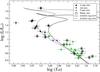 |
Fig. 1 HR diagram of the Hyades cluster. The two isochrones are calculated with the age given in WEBDA (log t = 8.9 – full line) and our best fit (log t = 8.8 – dashed line). |
The A stars were observed using SOPHIE, the échelle spectrograph at the Observatoire de Haute-provence (OHP). SOPHIE spectra stretch from 3820 to 6930 Å in 39 orders with two different spectral resolutions: the high-resolution mode HR (R = 75000) and the high-efficiency mode HE (R = 39000). All A stars were observed in the HR mode. The observing dates, exposure times, and signal-to-noise ratios achieved for each A star are collected in Table 2. On good nights, an exposure time of 25 min typically yielded well-exposed spectra with signal-to-noise ratios ranging from 300 to 600, depending on the V magnitude. As we did not get enough observing time to observe the F stars with SOPHIE as well, we used the mono-order AURELIE spectra obtained by Varenne & Monier (1999). For each F star, three spectral regions centred on λ6160 Å, λ5080 Å and λ5530 Å had been observed at resolutions 30 000 (V ≥ 6) or 60 000 (V ≤ 6) and signal-to-noise ratios close to 200.
The fundamental data for the selected stars are collected in Table 1. The van Bueren and Henry Draper identifications appear in Cols. 1 and 2, the spectral type retrieved from SIMBAD or from Abt & Morell (1995) in Col. 3, and the apparent magnitudes in Col. 4. Effective temperatures (Teff) and surface gravities (log g), derived from uvbyβ photometry (see Sect. 3), appear in Cols. 5 and 6. The derived projected rotational velocities and the microturbulent velocities are in Cols. 7 and 8. Comments about binarity and pulsation appear in the last column. The apparent rotational velocities range from 11 km s-1 to 165 km s-1, and only 7 stars rotate faster than 100 km s-1.
Inspection of the CCDM catalogue (Dommanget & Nys 1995) reveals that 13 of the 16 A stars are in binary or multiple systems. All of these stars are primaries and the components are much fainter (1 mag < Δm < 9.5 mag). Only the case of HD 27962 (CCDM J04255+1755 AB) has to be accounted for because its companion (component B) is three magnitudes fainter than A and at only 1.4′′ from A. In the case of F stars, 13 among the 28 stars belong to multiple systems. Six of them have nearby companions whose angular distance was probably less than the fiber angular size on the sky (3 arcsec) and who are only three magnitudes fainter than the brightest star we analysed. The spectral types of these companions are unknown. For the F stars, these are
-
HD 26015 = CCDM J04077+1510A has acompanion at about 4′′ with Δm = 2.8 mag;
-
HD 27383 = CCDM J04199+1631AB: components A and B are very close with Δm = 2.0 mag;
-
HD 27991 = CCDM J04257+1557AP: companion P is quoted as at 0.1′′ with Δm = 0.7 mag;
-
HD 28363 = CCDM J04290+1610AB is a spectroscopic binary whose angular separation is not specified with a Δm = 1.0 mag;
-
HD 30810 = CCDM J04512+1104AB is a triple star whose component B has same magnitude as A, but no angular separation is provided.
For these six stars, we believe that the light of the companions might have contaminated the spectra of the brightest components we analysed. The effects are probably most pronounced for the F stars HD 26015, HD 27383, HD 27991, HD 28363, and HD 30810.
The SOPHIE spectra were reduced using IRAF (Image Reduction and Analysis Facility, Tody 1993) to properly correct for scattered light. The sequence of IRAF procedures, which follows the method devised by Erspamer & North (2002), is fully described in Paper I.
Basic physical quantities for the programme stars.
3. Abundance analysis: method and input data
The abundances of 15 chemical elements were derived by iteratively adjusting synthetic spectra to the normalized spectra and minimizing the chi-square of the models to the observations. Spectrum synthesis is mandatory because the apparent rotational velocities range from 11 to 165 km s-1. Specifically, synthetic spectra were computed by assuming LTE with Takeda’s (1995) iterative procedure and double-checked using Hubeny & Lanz (1992) SYNSPEC48 code. This version of SYNSPEC calculates lines for elements up to Z = 99.
3.1. Atmospheric parameters and model atmospheres
The effective temperatures and surface gravities were determined using the UVBYBETA code developed by Napiwotzki et al. (1993). This code is based on the Moon & Dworetsky (1985) grid, which calibrates the uvbyβ photometry in terms of Teff and log g. The photometric data were taken from Hauck & Mermilliod (1998). The estimated errors on Teff and log g are ±125 K and ±0.20 dex, respectively (see Sect. 4.2 in Napiwotzki et al. 1993). The found effective temperatures, and surface gravities are collected in Table 1.
The ATLAS9 (Kurucz 1992) code was used to compute LTE model atmospheres assuming a plane-parallel geometry, a gas in hydrostatic and radiative equilibrium, and LTE. The ATLAS9 model atmospheres contain 64 layers with a regular increase in log τRoss = 0.125 and were calculated assuming Grevesse & Sauval (1998) solar chemical composition. This ATLAS9 version uses the new opacity distribution function (ODF) of Castelli & Kurucz (2003) computed for that solar chemical composition. Convection is calculated in the framework of the mixing length theory (MLT). We adopted Smalley’s prescriptions (Smalley 2004) for the values of the ratios of the mixing length to the pressure scale height ( ) and the microturbulent velocities (constant with depth).
3.2. The linelist
For the A stars, the line list used for spectral synthesis is the same as in Paper I. All transitions between 3000 and 7000 Å from Kurucz’s gfall.dat2 linelist were selected. The abundance analysis relies on more than 200 transitions for the 15 selected elements as explained in Paper I. The adopted atomic data for each element are collected in Table 8 of Paper I where, for each element, the wavelength, adopted oscillator strength, its accuracy (when available), and original bibliographical reference are given. The two Na lines at 5890 and 5896 Å were not used in this paper. These lines are likely to be affected by interstellar absorption and non-LTE effects, an LTE treatment assuming depth-independent microturbulence underestimates abundances (Takeda et al. 2009). For the F stars, the same line list was used except for Fe and Mg since only FeI and MgI lines are available in the AURELIE spectra. We used the same atomic data for these lines as those in Table 3 of Varenne & Monier (1999). Most of the lines studied here are weak lines formed deep in the atmosphere where LTE should prevail. They are well-suited to abundance determinations. We have also included data for hyperfine splitting for the selected transitions when relevant, using the linelist gfhyperall.dat3. However the moderate spectral resolution of the spectra and smearing out of spectra by stellar rotation clearly prevent us from detecting signatures of hyperfine splitting and isotopic shifts in our spectra.
3.3. Spectrum synthesis
For each modelled transition, the abundance was derived iteratively using Takeda’s (1995) procedure, which minimizes the chi-square between the normalized synthetic spectrum and the observed one. As explained in Paper I, Takeda’s code consists in two routines. The first routine computes the opacity data and is based on a modified version of Kurucz’s Width9 code (Kurucz 1992a) while the second computes the normalized flux and minimizes the dispersion between synthetic and observed spectra (see Paper I for a complete description of the method).
We first derived the rotational (vesini) and microturbulent (ξt) velocities using several weak and moderately strong FeII lines located within the range 4491.405−4508.288 Å, and the MgII triplet at 4480 Å by allowing small variations around solar abundances of Mg and Fe as explained in Sect. 3.2.1 of Paper I. The weak Fe lines are very sensitive to rotational velocity but not to microturbulent velocity while the moderately strong FeII lines are affected mostly by changes in microturbulent velocity. The MgII triplet is sensitive to both ξt and vesini. Once the rotational and microturbulent velocities were fixed, we then derived the abundance that minimized the chi-square for each transition of a given chemical element. These individual abundances may differ because of different levels of accuracies in the atomic data of each line and possibly because of deviations from LTE in a few of them. The derivation of the mean abundance from these individual abundances is explained in Sect. 3.5. The abundances were then double-checked using Hubeny & Lanz’s (1992) SYNSPEC48 code.
As an example, we display in Fig. 2 the final synthetic spectrum that best fits several Fe II lines in the observed spectrum of HD 28527 (A6IV) in the spectral interval 4513−4525 Å. In this region, the independent fit of each line yields only slightly different abundances. The displayed synthetic spectrum is computed for an Fe abundance of +0.30 dex, which is the derived mean value in HD 28527.
In the case of stars rotating faster than about 80 km s-1, the following neighbouring lines blend: Ti II 4394.059 Å and Ti II 4395.051 Å, Mn I 4033.062 Å and 4034.483 Å, and the O I lines “triplet” at 6155.900 Å, 6156.750 Å, and 6158.1 Å. In these cases, the abundances given in Table 8 (available at the CDS) are those that provide the best match to each blend.
Observing log for the A stars of the Hyades open cluster.
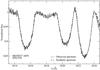 |
Fig. 2 A typical agreement between the observed spectrum (thin line) of HD 28527 (A6IV) and the synthetic spectrum (dashed thick line) computed as explained in Sect. 3. Three iron (FeII) lines calculated for [Fe/H] = +0.30 dex, the mean Fe abundance, are displayed in this figure. |
3.4. Internal consistency checks on the spectral energy distribution
For a few stars, we checked the fundamental parameter determinations by modelling the entire spectral energy distribution from far UV to IR with the theoretical ATLAS9 flux computed for the derived fundamental parameters and the individual abundances. Figure 3 exemplifies this check for HD 27819. The theoretical spectral energy distribution was computed with the LLmodel code (Shulyak et al. 2004). The observed spectral energy distribution was constructed from Adelman et al. (1989) spectrophotometry and IUE spectrophotometry: SWP04446 (low resolution) + LWP16605 (high resolution resampled to the LWP low resolution). The theoretical LLmodel spectral energy distribution, degraded to a spectral resolution comparable to that of the IUE low-resolution spectra, follows the overall shape of the observed flux distribution nicely, which lends credence to the adopted fundamental parameters and the derived abundances.
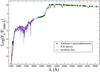 |
Fig. 3 Comparison of the LLmodel theoretical spectral energy distribution of HD 27819 with the observed spectrophotometry of HD 27819 in the UV and the optical. |
3.5. Mean abundances and uncertainties
Both apparent rotational and microturbulent velocity were determined for all sample stars. The abundances of 15 chemical elements were determined for most of the stars (when the selected lines were accessible with good signal-to-noise ratios). The abundances for A and F stars are collected in Tables 5 and 6 (available at the CDS). These abundances are relative to the Sun4. Solar abundances are from Grevesse & Sauval (1998). For each chemical element, the final abundance is an average of the abundances derived from each line. The errors on the final abundances (labelled as σ) are standard deviation assuming a Gaussian distribution of the abundances derived from each line:
 (1)
(1) (2)where
  is the mean value of the abundance, N the number of lines of the element, and σ the standard deviation.
Accordingly, the error on the abundance of a given element depends on the individual abundances derived from each line and usually varies from star to star. When only one transition was used to derive the abundance (for CI, OI5, MgI, SiII, CaII, ScII, and YII in F stars), the corresponding error was computed according to the formulation explained in Appendix A of Paper I. It consists of perturbing each of the 6 nominal parameters (Teff, log g, ξt, vesini, log gf, and the continuum position) and repeating the fit for each line. The perturbation Δ(Teff) is 200 K and Δ(log g) is 0.20 dex (Napiwotzki et al. 1993), Δ(ve sin i) is estimated as 5% of the nominal vesini, and Δ(ξt) is 1 km s-1 (Gebran 2007) Concerning the oscillator strengths, Δ(log gf) depends on the accuracy of the considered lines, and varies from 3% to more than 50%. For more details concerning the accuracies of the oscillator strengths, see Table 8 (3rd column) of Paper I and Table 3 (3rd column) of Varenne & Monier (1999). The continuum placement error depends on the rotational velocity of the star and is fully explained in Paper I.
The difference between the nominal abundance and the one derived with the perturbated parameter yields the uncertainty assigned to the given parameter. Considering that the errors are independent, the upper limit of the total uncertainty σtoti for a given transition (i) is  (3)Table 8 collects the abundances derived for each transition for each studied element in all A and F stars including Procyon (F5V) which served as control star for the spectral synthesis. The absolute values are represented in this table (log (X/H) ⋆ + 12), and the wavelengths are in Å.
4. Results
We first tested the spectrum synthesis on Procyon whose abundances are almost solar (Steffen 1985). For elements having lines on the 3 AURELIE spectral ranges, abundances agree well. The derived abundances are displayed in Fig. 4. We found nearly solar abundances for all the elements except for Sr. The differences between the abundances we derived and those derived by Steffen (1985) are depicted as squares in Fig. 4. They are less than 0.10 dex for 13 out of 15 elements and less than 0.15 dex for the remaining (Ni and Zr), typically less then the order of magnitude of the uncertainties. We found an apparent rotational velocity of 6 km s-1 and a microturbulent velocity of 2.2 km s-1, in good agreement with Steffen’s values (vesini = 4.5 km s-1 and ξt = 2.1 km s-1, Steffen 1985).
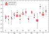 |
Fig. 4 Comparison of the abundances determined in this study and the one derived by Steffen (1985; S85) for Procyon (red squares). The derived abundances are in black circles. |
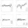 |
Fig. 5 Abundance patterns for the “normal” A a), Am b), and F c,d) stars of the Hyades cluster. |
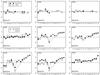 |
Fig. 6 Comparisons between the abundances derived in this work (filled circles), Varenne & Monier (1999; VM99, open squares), Hui-Bon-Hoa & Alecian (1998; HA98, filled diamonds), and Burkhart & Coupry (2000; BC00, open triangles) for 9 stars of the Hyades cluster. |
4.1. Abundance patterns and comparison with previous studies
Abundance patterns graphs where abundances are displayed against atomic number Z are particularly useful for comparing the behaviour of A, Am, and F stars for different chemical elements. The abundance patterns for A, Am and F stars are displayed in Figs. 5a−d. The pattern for A stars resembles that of the A stars in Coma Berenices and in the Pleiades (Papers I and II). Among the 9 A stars, the elements that exhibit the largest star-to-star variations are Sr, Y, and Zr (1.0 to 0.8 dex), while C and Cr display the lowest variations (0.2 dex). The amplitudes of variations for the other elements, O, Na, Mg, Si, Ca, Sc, Ti, Mn, Fe, and Ni range from 0.25 to 0.60 dex (see further discussion of individual elements).
The 7 Am stars display the characteristic jigsaw pattern with larger excursions around the solar composition than the A stars show. Almost all Am stars are heavily deficient in Sc, but not all are deficient in Ca, and the deficiencies are more modest for this element. Almost all are more deficient in C and O than the A stars, and all are more enriched in iron-peak elements and heavy elements (Sr and beyond). For all chemical elements, the star-to-star variations of Am stars are usually greater than for the A stars.
In contrast, F stars exhibit little scatter around the mean abundances. For clarity, the abundances of F stars are sorted out in two graphs: the data for stars cooler than 6600 K appear in Fig. 5c and for those hotter than 6600 K in Fig. 5d. At the age of the Hyades, an F star with a temperature of 6600 K has a 1.3−1.4 M⊙ mass. As explained in Sect. 5.1.2, the evolutionary models show that the effects of atomic diffusion are more pronounced in all stars earlier than F5 (M ⋆ > 1.3 M⊙) (Turcotte et al. 1998a). Sorting out the F stars into two groups (Teff < 6600 K and Teff ≥ 6600 K) helps to highlight the occurrence of diffusion in the most massive F stars.
Graphically, we compared the abundances derived in this study with previous determinations for 9 stars in Fig. 6. The abundances of Mg, Ca, Sc, Cr, Fe, and Ni derived by Hui-Bon-Hoa & Alecian (1998) for HD 27819, HD 27962, and HD 30210 are depicted as losanges, the abundances of Si and Fe in HD 27819 and HD 30210 derived by Burkhart & Coupry (2000) as empty triangles and those of C, O, Na, Mg, Si, Ca, Sc, Fe, Ni, and Y derived by Varenne & Monier (1999). For all stars, the overall shapes of the abundance patterns agree well. Differences exist for individual elements mostly because of using different microturbulent velocities, rotational velocities, and in the case of A stars, different ionization levels.
We have also compared the derived Fe abundances for F stars in this work with the compilation available in Perryman et al. (1998) in Table 3. The [Fe/H] determinations come from Chaffee et al. (1971) (CCS), Boesgaard & Budge (1988) (BB), Boesgaard (1989) (B) and Boesgaard & Friel (1990) (BF), they mostly rely on adjustments of theoretical equivalent widths to observed ones. Differences arise from the use of different effective temperatures with a fixed gravity (log g = 4.5 dex), older version of Kurucz ATLAS model atmospheres, different microturbulent velocities (determined using Nissen’s 1981 fit), and different neutral Fe lines.
4.2. Comments on particular stars
Am stars are expected to be underabundant in light elements, underabundant in Ca and/or Sc, as well as overabundant in iron-peak and heavy elements. HD 27962 is the hottest A star in the Hyades, and Mermilliod (1982) suggested that it may be a blue straggler based on its location on the HR diagram. Conti (1965) classified HD 27962 as an Am star based on the weakness of the Sc line at λ4246 Å and the strength of Sr line at λ4215 Å. Abt (1985) assigned a spectral type Am (A2KA3HA5M) to HD 27962. Our analysis shows that Sc is deficient by −0.90 dex and that iron-peak and heavy elements are enhanced in this star so that it has the characteristics of an Am star. Our analysis of HD 28355 (A7V/A5m) also confirms its Am status as Sc is deficient by −1.05 dex, and iron-peak and heavy elements are enhanced. Hauck (1977) had previously classified HD 28355 as an Am star on the basis of Geneva photometry. Both HD 27962 and HD 28355 are classified as Am in the catalogue of Renson (1992). The seven stars represented in Fig. 5b are classified as Am in the catalogue of Renson (1992). The abundances of all these stars except HD 29499 display the characteristic jigsaw pattern of Am stars: underabundances of light elements, of Ca, and/or Sc and overabundances of metals and heavy elements. Our abundance analysis strongly suggests that HD 29499 (A5m) may actually be a normal A star: it does not have Ca nor Sc deficiencies and is only moderately enriched in iron-peak and heavy elements. Its apparent rotational velocity is around 60 km s-1, which is rather large for an Am star. Abt & Morrell (1995) have classified HD 29499 as a giant star with metallic lines (A9III) but the surface gravity we found for HD 29499 suggests that it is still on the main sequence.
Iron abundance comparisons.
4.3. Behaviour of the abundances of individual elements
As we did for the Coma Berenices cluster (see Paper I), the behaviour of the found abundances has been studied versus apparent rotational velocity (ve sin i) and effective temperature (Teff). Any correlation/anticorrelation would be very valuable to theorists investigating the various hydrodynamical mechanisms affecting photospheric abundances. As we emphasized in Paper I, the existence of star-to-star variations with fundamental parameters can be established independently of errors in the absolute values of the oscillator strengths, since all stars will be affected in the same manner.
Second, we searched whether the abundances of individual elements correlate with that of Fe. We expect the abundances of Fe, Ti, O, Cr, Mg, Mn, C, Ca, and Ni to be fairly reliable as we synthesized several lines of quality A to D for these elements. For Y and Zr, several lines are available, but their accuracy is unknown, so the abundances of these elements should be taken with caution. The abundances of Sr, derived from 2 transitions whose oscillator strengths have unknown inaccuracies, are likely to be inaccurate.
Abundances are displayed against Teff in the left part of Figs. 8 to 12. Inspection of these figures reveal that there is no systematic slope (positive nor negative) for several chemical elements. A stars display star-to-star variations in abundances larger than the typical uncertainty. Table 4 presents the mean abundance, the standard deviation and maximum spread for all chemical elements in F, A (normal and Am), and Am stars. Scatter around the mean value is more important in A stars than in F stars, namely for C, Na, Sc, Fe, Ni, Sr, Y, and Zr. This behaviour has already been found in Coma Berenices and the Pleiades (see Papers I and II).
The abundances of C, O, Mg, Sc, Fe, and Y are displayed versus ve sin i for A, Am, and F stars in Fig. 7. For a given element, there is usually a considerable scatter in abundances at a given rotation rate. None of the derived abundances in this study exhibits a clear correlation or anticorrelation with ve sin i. Charbonneau & Michaud (1991) have analysed the effect of meridional circulation on the chemical separation of elements in rotating stars. They showed that, for stars rotating at less than ve sin i ≤ 100 km s-1, no correlation should be expected between abundances and apparent rotational velocities. This prediction is verified by our findings (see Fig. 7). Even if we distinguish two velocity regimes (ve sin i ≤ 100 km s-1 and ve sin i ≥ 100 km s-1), we fail to find any dependence between the abundances of any of the 15 chemical elements and the apparent rotational velocity. Recently, Takeda et al. (2008) find that the peculiarities (underabundances of C, O, and Ca) seen in slow rotators efficiently decrease with an increase in rotation and almost disappear at ve sin i ≥ 100 km s-1. We confirm that for these chemical elements, abundance anomalies vanish at ve sin i ≥ 100 km s-1.
Mean abundances and dispersions.
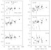 |
Fig. 7 Abundances of C, O, Mg, Sc, Fe, and Y versus vesini for A, Am, and F stars. |
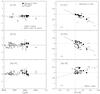 |
Fig. 8 Left panel: abundances of C, O, and Na versus effective temperature. The dotted line corresponds to the solar value and the dashed line to the mean value determined for the F stars of the cluster. Right panel: [C/Fe], [O/Fe], and [Na/H] versus [Fe/H]. The filled dots correspond to normal A stars, the open squares correspond to Am stars, and the filled diamonds to F stars. In the plot representing [Na/H] versus [Fe/H], the dashed line corresponds to the solar [Na/Fe] ratio. The error bars in the right panel represent the mean standard deviation for the displayed abundances. |
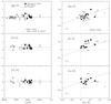 |
Fig. 9 Left panel: abundances of Mg, Si, and Ca versus effective temperature. The dotted line represents the solar value and the dashed one represents the mean abundance of F stars. Right panel: [Mg/H], [Si/Fe], and [Ca/H] versus [Fe/H]. The symbols are the same as in Fig. 8. The dashed lines represent the solar ratios. |
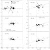 |
Fig. 10 Left panel: abundances of Sc, Ti, and Cr versus effective temperature. The dotted line represents the solar value and the dashed one represents the mean abundance of F stars. Right panel: [Sc/H], [Ti/Fe], and [Cr/H] versus [Fe/H]. The symbols are the same as in Fig. 8. The dashed lines represent the solar ratios. |
Carbon and O abundances display large star-to-star variation in A stars. No clear correlation was found between the abundances of C or O and [Fe/H]. However, both [C/Fe] and [O/Fe] are anticorrelated with [Fe/H]. For the C lines used in our study, non-LTE abundance corrections for the A stars (7000 K < Teff < 10 000 K) are expected to be negative (Rentzsch-Holm 1996) and do not affect the star-to-star dispersion in [C/H]. Non-LTE corrections for O abundances are negligible in the case of the OI lines considered here (see Paper I). Carbon and O tend to be more deficient in Am stars than in A stars of similar effective temperatures or rotation rates.
For A stars, Na abundances appear to be slightly correlated to the Fe abundances as seen in Fig. 8. We find important star-to-star abundance variations in [Na/H]. In Fig. 9, the scatter of [Mg/H] for both F and A stars does not exceed the typical uncertainty (0.20 dex), which suggests that there are no significant star-to-star variations in Mg abundances. As mentioned in Paper I, the MgII λ4481 Å triplet yields higher abundances than other MgII lines, therefore we excluded this line from our analysis. The corrected [Mg/H] abundances appear to be slightly correlated with [Fe/H]. The ratio [Mg/Fe] is close to solar for the A stars. The Si lines synthesized in this work have low-quality oscillator strengths and have not been updated for the recent values of the log gf of the NIST6 database. The systematic overabundances could be due to incorrect oscillator strengths, therefore the Si abundances should be viewed with caution. There does not seem to be any significant star-to-star variation in [Si/H].
Calcium abundance exhibit neither real star-to-star variations or any clear correlation with repsect to [Fe/H]. Not all Am stars are underabundant in Ca, and only two of the 7 Am stars exhibit large underabundances in Ca. This result differs from Varenne & Monier’s (1999) findings because of using different microturbulent velocities and ionization levels as explained in Sect. 4.1. In Varenne & Monier (1999), the derived microturbulent abundances were larger (up to 5 km s-1) than those derived here, leading to lower abundances of Ca. Star-to-star variations in Sc abundance are clearly present for A stars (Fig. 10). Scandium is the most scattered of all analysed elements, and they do not appear to be correlated to Fe abundances for either A and F stars. All Am stars except for HD 29499 are deficient in Sc and fall in the lower right part of Fig. 10. The two stars, HD 27962 and HD 28355, for which we confirm the status as Am stars, are located in that region.
Titanium, Cr, and Mn abundances were derived only for A stars since none of the Ti, Cr, and Mn lines observed with AURELIE have oscillator strengths accurate enough to determine abundances. There does not seem to be significant star-to-star variation in [Ti/H], [Cr/H], or [Mn/H] for the A stars (Fig. 10). The Ti abundances of the Hyades A stars do not appear to be correlated with the Fe abundances. The Cr abundance appears to only be loosely correlated to that of Fe.
Iron abundances have been derived for all F and A stars in our sample. Neutral Fe lines were used for F stars yielding a mean abundance of ⟨ [ Fe/H ] ⟩ F = 0.05 ± 0.05 dex. This value, which represents the average metallicity of the cluster, is almost 0.1 dex smaller than the value derived by Boesgaard & Friel (1990) from a different sample of 14 F dwarfs (+0.127 ± 0.022 dex using different FeI lines from ours). For the 16 A stars, 27 lines of FeII were synthesized. The normal A and Am stars scatter around their mean abundance with a maximum spread of about 0.50 dex, which is more than twice more than the typical uncertainty on [Fe/H] of about 0.20 dex. This suggests real star-to-star variations in [Fe/H] among the Hyades A stars. Nickel behaves similarly to Fe (see Fig. 11), because the A stars display large star-to-star variations in [Ni/H] and the abundances are clearly correlated with the Fe abundances, because the correlation coefficient is close to 1.
All Am stars appear to be overabundant in Sr. Star-to-star variation in [Sr/H] are clearly present. Strontium abundances are only loosely correlated with those of Fe (right part of Fig. 12). Yttrium and Zr are found to be overabundant in all A stars with real star-to-star variations in [Y/H] and [Zr/H] (Fig. 12). As for Sr, Y, and Zr abundances are correlated to [Fe/H] but appear to increase more rapidly than [Fe/H] (slope of 1.8 for Y and 2.1 for Zr).
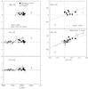 |
Fig. 11 Left panel: abundances of Mn, Fe, and Ni versus effective temperature. The dotted line represents the solar value and the dashed one represents the mean abundance of F stars. Right panel: [Mn/H] and [Ni/H] versus [Fe/H]. The symbols are the same as in Fig. 8. The dashed lines represent the solar ratios. |
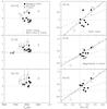 |
Fig. 12 Left panel: abundances of Sr, Y, and Zr versus effective temperature. Right panel: [Sr/H], [Y/Fe], and [Zr/H] versus [Fe/H]. The symbols are the same as in Fig. 8. |
5. Discussion
5.1. Self-consistent evolutionary models
The derived abundances have been compared to the predictions of recent evolutionary models. These models are calculated with the Montréal stellar evolution code. The chemical transport problem is treated with all known physical processes from first principles, which include radiative accelerations, thermal diffusion, and gravitational settling (for more details see Turcotte et al. 1998b; Richard et al. 2001, and references therein). These models follow the chemical evolution of most elements, as well as some isotopes up to Z ≤ 28 (28 species in all). As the abundances change, the Rosseland opacity and radiative accelerations are continuously recalculated at each mesh point and for every time step during evolution, which means that the treatment of particle transport is completely self-consistent. The spectra used to calculate the monochromatic opacities are taken from the OPAL database (Iglesias et al. 1996). The radiative accelerations are calculated as described in Richer et al. (1998) with corrections for the redistribution of momentum from Gonzalez et al. (1995) and LeBlanc et al. (2000). The mixing length parameter and initial He abundance (α = 2.096 and Y0 = 0.2779, respectively) are calibrated to fit the current luminosity and radius of the Sun (see Turcotte et al. 1998b, model H). Models are evolved from the pre-main sequence with a solar scaled abundance mix. The initial abundance ratios are given in Table 1 of Turcotte et al. (1998b). For the initial mass fraction of metals we used both Z0 = 0.02, the solar metal content, and Z0 = 0.024 (to represent the increased metallicity of the Hyades, Lebreton et al. 2001).
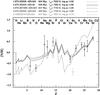 |
Fig. 13 Comparison of the predicted surface abundances for stars of 1.8, 2.0, and 2.15 M⊙ with different turbulence prescriptions and different initial metallicities with those derived (depicted as diamonds with their respective uncertainties) for the Am star HD 30210 (Teff = 8082 K and log g = 3.92). The grey symbol for Sc indicates that it is not considered in the evolutionary models. |
5.1.1. The A stars
The derived abundances in A stars are compared to the predictions of self-consistent evolutionary models calculated as in Richer et al. (2000). These models include an arbitrary parameter, the amount of mass mixed by turbulent mixing, in order to lower the effects of chemical separation and better fit the abundances of AmFm stars. The effect of turbulence is to extend the mixed mass below the surface convection zone, down to layers where atomic diffusion is less efficient (i.e. where time scales are longer owing to higher local density). A priori, the cause of turbulence is not considered. However, it was found to be compatible with rotationally induced turbulence as calculated by Zahn (2005) and Talon et al. (2006). The surface abundances are shown to depend solely on the amount of mass mixed, as well as initial metallicity. In Fig. 13, we compare the predicted surface abundances for five models with masses of 1.8, 2.0, and 2.15 M⊙ to the observed abundances of the Hyades A2m star HD 30210 (Teff = 8082 K and log g = 3.92 dex). The models are shown for both Z = 0.02 and Z = 0.024. To help interpret the chosen nomenclature, the 2.0T5.3D1000-3 corresponds to a 2.0 M⊙ star for which the abundances are completely homogenized down to log T = 5.3. Below this point, as we move deeper inside the star, the turbulent diffusion coefficient DT = 1000DHe (the He diffusion coefficient) decreases as ρ-3 (2.0T5.3D25K-3 would have the same behaviour except that the turbulent coefficient DT = 25000DHe at log T = 5.3). It is clear from the plot that the amount of prescribed turbulence has an influence on the surface behaviour. The model 2.0T5.3D1000-3 does not sufficiently impede microscopic diffusion to reproduce most abundances. However, for all other models with greater turbulence, the predicted C and O underabundances are not as important as the observed anomalies. The predicted slight underabundances of Na, Mg, and Si are not observed in HD 30210, but are observed in a few of the Am stars, however, the Si abundance is probably too large. The model that best fits the data is 2.15T5.3D25K-3Z0.024, which has a turbulence prescription, which in turn was just as able to reproduce the observations in Coma Berenices (see Figs. 14 and 15 of Paper I). As in Paper I, models with less turbulence roughly replicate the observations for Z < 12, and the more turbulent models are better able to reproduce the heavier elements (Z > 15). The different metallicities do not lead to significant differences in the predicted abundance patterns, but do have a strong effect on Teff.
5.1.2. The F-type stars
For the F dwarfs, we compared the found abundances to the predicted surface abundances for C, O, Na, Mg, Fe, and Ni using Turcotte’s evolutionary models at 620 Myr (Turcotte et al. 1998a). These models, calculated for masses ranging from 1.1−1.5 M⊙, treat radiative diffusion in detail but do not include macroscopic mixing processes (meridional circulation, turbulence, or mass loss). They show that the effects of atomic diffusion, namely the appearance of surface abundance anomalies, can be expected in all stars earlier than F5 (M∗ > 1.3 M⊙).
The found mean C abundance for F stars, ⟨ [C/H] ⟩ = −0.09 dex with very small dispersion, does not agree with predicted underabundance at 620 Myr (log age = 8.79 in Fig. 7 of Turcotte et al. 1998a) and for a 1.4 M⊙ star, representative of the F stars analysed here. The O abundances, which show large scatter for the F stars, can typically be underabundant by −0.41 dex or overabundant by up to 0.28 dex for a 1.4 M⊙ F star (roughly an effective temperature of 6700 K at the age of the Hyades). Again, they do not agree with the predicted surface underabundances [O/H] predicted by Turcotte et al. (1998a). The predicted solar Na abundances match our determinations for F stars reasonably well. Magnesium is predicted to be slightly underabundant (Fig. 7 of Turcotte et al. 1998a), whereas for most F stars we find overabundances. Finally, Fe and Ni are found to be mildly overabundant for F stars with Teff ∈ [6600 K, 6800 K] (⟨ [Fe/H] ⟩ = 0.06 dex and ⟨ [Ni/H] ⟩ = 0.11 dex). These results disagree with the overabundances of 0.5 and 0.8 dex for 1.4 M⊙. As expected, these purely diffusive models typically predict too little C and O and too many iron-peak elements.
6. Conclusion
Selected high-quality lines in new high-resolution échelle spectra of 16 A and 28 F stars of the Hyades were synthesized in a uniform manner to derive LTE abundances, a few of which have been corrected for non-LTE effects whenever possible. Even when binary stars are removed, the abundances of several chemical elements for A stars and early F stars exhibit real star-to-star variations, significantly larger than for the late F stars. The broadest spreads occur for Sc, Sr, Y, and Zr while the narrowest are for Mg, Si, and Cr for A stars. Gebran et al. (2008) and Gebran & Monier (2008) already find similar behaviour in the Coma Berenices and the Pleiades. The derived abundances do not depend on either effective temperatures or apparent rotational velocities as expected since the timescales of diffusion are much shorter than those of rotational mixing (Charbonneau & Michaud 1991). The abundances of Cr, Ni, Sr, Y, and Zr are correlated with the Fe abundance as found for the Pleiades and Coma Berenices. The ratios [C/Fe] and [O/Fe] are anticorrelated with [Fe/H] (particularily true for normal A stars). Compared to normal A stars, all Am stars in the Hyades appear to be more deficient in C and O and more overabundant in elements heavier than Fe but not all are deficient in Ca and/or Sc. The F stars have nearly solar abundances for almost all elements except for Si and Ca. The blue straggler HD 27962 appears to have abundances characteristic of an Am star (Sc deficiency and enrichment in iron-peak and heavy elements). Conversely, our abundance analysis of HD 29499 (A5m) yields normal abundances in Ca and Sc and only moderate enrichment in iron-peak and heavy elements suggesting that this star might be a normal A star. The detailed modelling of the A2m star HD 30210 including radiative diffusion and different amounts of turbulent diffusion reproduces the overall shape of the abundance pattern for this star but not individual abundances. Models with the least turbulence reproduce the abundances of the lightest (Z < 12) and those with most turbulence reproduce abundances of elements with Z > 15. For a few elements, the discrepancies between derived and predicted abundances could come from non-LTE effects. However, including competing processes such as different prescriptions of rotational mixing (Zahn 2005) and/or different amounts of mass loss (Vick et al. 2010) could improve the agreement between observed and predicted abundance patterns.
www.univie.ac.at/webda/
![Mathematical equation: $\left(\rm \left[\frac{X}{H}\right]=\log \left(\frac{X}{H}\right)_{\star}-\log \left(\frac{X}{H}\right)_{\odot}\right)$](/articles/aa/full_html/2010/15/aa13273-09/aa13273-09-eq97.png) .
.
Oxygen lines are blended in F stars because of the low resolution of AURELIE spectra, which is not the case of SOPHIE’s A stars.
Acknowledgments
We warmly thank the OHP night staff for their support during the observing runs. This research has used the SIMBAD, WEBDA, VALD, NIST, and Kurucz databases. M.V. thanks the Département de physique at l’Université de Montréal, as well as the GRAAL at l’Université Montpellier II, for financial support and the Réseau Québécois de Calcul de Haute Performance (RQCHP) for providing us with the computational resources required for this work. Special thanks go to Georges Michaud and Olivier Richard for their careful reading of the manuscript and useful suggestions. L.F. received support from the Austrian Science Foundation (FWF project P17890-N2).
References
- Abt, H. A., & Morrell, N. I. 1995, ApJS, 99, 135 [Google Scholar]
- Adelman, S. J., Pyper, D. M., Shore, S. N., White, R. E., & Warren, W. H. 1989, A&AS, 81, 221 [Google Scholar]
- Alecian, G. 1996, A&A, 310, 872 [NASA ADS] [Google Scholar]
- Balona, L. A. 1994, MNRAS, 268, 119 [NASA ADS] [CrossRef] [Google Scholar]
- Barrado y Navascues, D., & Stauffer, J. R. 1996, A&A, 310, 879 [NASA ADS] [Google Scholar]
- Burkhart, C., & Coupry, M. F. 2000, A&A, 354, 216 [NASA ADS] [Google Scholar]
- Boesgaard, A. M. 1989, ApJ, 336, 798 [NASA ADS] [CrossRef] [Google Scholar]
- Boesgaard, A. M., & Tripicco, M. J. 1986, ApJ, 303, 724 [NASA ADS] [CrossRef] [Google Scholar]
- Boesgaard, A. M., & Budge, K. G. 1988, ApJ, 332, 410 [NASA ADS] [CrossRef] [Google Scholar]
- Boesgaard, A. M., & Friel, E. D. 1990, ApJ, 351, 467 [Google Scholar]
- Castellani, V., Degl’Innocenti, S., Pra da Moroni, P. G., & Tordiglione, V. 2002, MNRAS, 334, 193 [NASA ADS] [CrossRef] [Google Scholar]
- Cayrel, R., Cayrel, G., Campbell, B., & Dappen, W. 1984, Observational Tests of the Stellar Evolution Theory, 105, 537 [NASA ADS] [Google Scholar]
- Cayrel de Strobel, G., Crifo, F., & Lebreton, Y. 1997, Hipparcos – Venice ’97, 402, 687 [Google Scholar]
- Cayrel de Strobel, G., Soubiran, C., & Ralite, N. 2001, A&A, 373, 159 [NASA ADS] [CrossRef] [EDP Sciences] [Google Scholar]
- Castelli, F., & Kurucz, R. L. 2003, IAU Symp., 210, 20P [Google Scholar]
- Chaffee, F. H., Jr.,Carbon, D. F., & Strom, S. E. 1971, ApJ, 166, 593 [NASA ADS] [CrossRef] [Google Scholar]
- Charbonneau, P., & Michaud, G. 1991, ApJ, 370, 693 [NASA ADS] [CrossRef] [Google Scholar]
- Conti, P. S. 1965, ApJ, 142, 1594 [NASA ADS] [CrossRef] [Google Scholar]
- Dommanget, J., & Nys, O. 1995, Bulletin d’Information du Centre de Données Stellaires, 46, 3 [Google Scholar]
- Erspamer, D., & North, P. 2002, A&A, 383, 227 [NASA ADS] [CrossRef] [EDP Sciences] [Google Scholar]
- Friel, E. D., & Boesgaard, A. M. 1990, ApJ, 351, 480 [NASA ADS] [CrossRef] [Google Scholar]
- Garcia Lopez, R. J., Rebolo, R., Herrero, A., & Beckman, J. E. 1993, ApJ, 412, 173 [NASA ADS] [CrossRef] [Google Scholar]
- Gebran, M. 2007, Ph.D. Thesis, UMII [Google Scholar]
- Gebran, M., & Monier, R. 2008, A&A, 483, 567 [NASA ADS] [CrossRef] [EDP Sciences] [Google Scholar]
- Gebran, M., Monier, R., & Richard, O. 2008, A&A, 479, 189 [NASA ADS] [CrossRef] [EDP Sciences] [Google Scholar]
- Gigas, D. 1988, A&A, 192, 264 [NASA ADS] [Google Scholar]
- Gonzalez, J.-F., LeBlanc, F., Artru, M.-C., & Michaud, G. 1995, A&A, 297, 223 [NASA ADS] [Google Scholar]
- Grenon, M. 2000, HIPPARCOS and the Luminosity Calibration of the Nearer Stars, 24th meeting of the IAU, Joint Discussion 13, August, Manchester, England, meeting abstract, 13 [Google Scholar]
- Grevesse, N., & Sauval, A. J. 1998, Space Sci. Rev., 85, 161 [NASA ADS] [CrossRef] [Google Scholar]
- Griffin, R. F., Griffin, R. E. M., Gunn, J. E., & Zimmerman, B. A. 1985, AJ, 90, 609 [NASA ADS] [CrossRef] [Google Scholar]
- Hauck, B. 1977, Rev. Mex. Astron. Astrofis., 2, 231 [NASA ADS] [Google Scholar]
- Hauck, B., & Mermilliod, M. 1998, A&AS, 129, 431 [NASA ADS] [CrossRef] [EDP Sciences] [Google Scholar]
- Hill, G. M. 1995, A&A, 294, 536 [NASA ADS] [Google Scholar]
- Hill, G. M., & Landstreet, J. D. 1993, A&A, 276, 142 [NASA ADS] [Google Scholar]
- Holmberg, J., Nordström, B., & Andersen, J. 2007, A&A, 475, 519 [NASA ADS] [CrossRef] [EDP Sciences] [MathSciNet] [Google Scholar]
- Holweger, H., Steffen, M., & Gigas, D. 1986, A&A, 163, 333 [NASA ADS] [Google Scholar]
- Hubeny, I., & Lanz, T. 1992, A&A, 262, 501 [NASA ADS] [Google Scholar]
- Hui-Bon-Hoa, A., & Alecian, G. 1998, A&A, 332, 224 [NASA ADS] [Google Scholar]
- Iglesias, C. A., & Rogers, F. J. 1996, ApJ, 464, 943 [NASA ADS] [CrossRef] [Google Scholar]
- Kurucz, R. L. 1992, Rev. Mex. Astron. Astrofis., 23, 45 [Google Scholar]
- Lambert, D. L., McKinley, L. K., & Roby, S. W. 1986, PASP, 98, 927 [NASA ADS] [CrossRef] [Google Scholar]
- Landstreet, J. D., Bagnulo, S., Andretta, V., et al. 2007, A&A, 470, 685 [NASA ADS] [CrossRef] [EDP Sciences] [Google Scholar]
- LeBlanc, F., Michaud, G., & Richer, J. 2000, ApJ, 538, 876 [NASA ADS] [CrossRef] [Google Scholar]
- Lebreton, Y., Fernandes, J., & Lejeune, T. 2001, A&A, 374, 540 [NASA ADS] [CrossRef] [EDP Sciences] [Google Scholar]
- Lemke, M. 1989, A&A, 225, 125 [Google Scholar]
- Lemke, M. 1990, A&A, 240, 331 [Google Scholar]
- Marigo, P., Girardi, L., Bressan, A., et al. 2008, A&A, 482, 883 [NASA ADS] [CrossRef] [EDP Sciences] [Google Scholar]
- Monier, R. 2005, A&A, 442, 563 [NASA ADS] [CrossRef] [EDP Sciences] [Google Scholar]
- Moon, T. T., & Dworetsky, M. M. 1985, MNRAS, 217, 305 [NASA ADS] [CrossRef] [Google Scholar]
- Napiwotzki, R., Schoenberner, D., & Wenske, V. 1993, A&A, 268, 653 [NASA ADS] [Google Scholar]
- Nissen, P. E. 1981, A&A, 97, 145 [NASA ADS] [Google Scholar]
- Percival, S. M., Salaris, M., & Kilkenny, D. 2003, A&A, 400, 541 [NASA ADS] [CrossRef] [EDP Sciences] [Google Scholar]
- Perryman, M. A. C., Brown, A. G. A., Lebreton, Y., et al. 1998, A&A, 331, 81 [NASA ADS] [Google Scholar]
- Renson, P. 1992, Bulletin d’Information du Centre de Données Stellaires, 40, 97 [Google Scholar]
- Rentzsch-Holm, I. 1996, A&A, 312, 966 [NASA ADS] [Google Scholar]
- Rentzsch-Holm, I. 1997, A&A, 317, 178 [Google Scholar]
- Richard, O., Michaud, G., & Richer, J. 2001, ApJ, 558, 377 [NASA ADS] [CrossRef] [Google Scholar]
- Richer, J., Michaud, G., Rogers, F., et al. 1998, ApJ, 492, 833 [NASA ADS] [CrossRef] [Google Scholar]
- Richer, J., Michaud, G., & Turcotte, S. 2000, ApJ, 529, 338 [NASA ADS] [CrossRef] [Google Scholar]
- Salaris, M., Weiss, A., & Percival, S. M. 2004, A&A, 414, 163 [NASA ADS] [CrossRef] [EDP Sciences] [Google Scholar]
- Shulyak, D., Tsymbal, V., Ryabchikova, T., Stütz, Ch., & Weiss, W. W. 2004, A&A, 428, 993 [NASA ADS] [CrossRef] [EDP Sciences] [Google Scholar]
- Smalley, B. 2004, IAU Symp., 224, 131 [NASA ADS] [CrossRef] [Google Scholar]
- Solano, E., & Fernley, J. 1997, A&AS, 122, 131 [NASA ADS] [CrossRef] [EDP Sciences] [Google Scholar]
- Steffen, M. 1985, A&AS, 59, 403 [NASA ADS] [CrossRef] [MathSciNet] [PubMed] [Google Scholar]
- Takeda, Y. 1995, PASJ, 47, 287 [NASA ADS] [Google Scholar]
- Takeda, Y., & Sadakane, K. 1997, PASJ, 49, 367 [NASA ADS] [Google Scholar]
- Takeda, Y., Han, I., Kang, D.-I., Lee, B.-C., & Kim, K.-M. 2008, J. Kor. Astron. Soc., 41, 83 [Google Scholar]
- Takeda, Y., Kang, D.-I., Han, I., Lee, B.-C., & Kim, K.-M. 2009, PASJ, 61, 1165 [NASA ADS] [Google Scholar]
- Talon, S., Richard, O., & Michaud, G. 2006, ApJ, 645, 634 [NASA ADS] [CrossRef] [Google Scholar]
- Taylor, B. J. 2006, AJ, 132, 2453 [NASA ADS] [CrossRef] [Google Scholar]
- Thorburn, J. A., Hobbs, L. M., Deliyannis, C. P., & Pinsonneault, M. H. 1993, ApJ, 415, 150 [NASA ADS] [CrossRef] [Google Scholar]
- Turcotte, S., Richer, J., & Michaud, G. 1998a, ApJ, 504, 559 [NASA ADS] [CrossRef] [Google Scholar]
- Turcotte, S., Richer, J., Michaud, G., Iglesias, C. A., & Rogers, F. J. 1998b, ApJ, 504, 539 [NASA ADS] [CrossRef] [Google Scholar]
- van Leeuwen, F. 2007, Astrophys. Space Sci. Libr., 350, [Google Scholar]
- Varenne, O. 1999, A&A, 341, 233 [NASA ADS] [Google Scholar]
- Varenne, O., & Monier, R. 1999, A&A, 351, 247 [NASA ADS] [Google Scholar]
- Vick, M., Michaud, G., Richer, J., & Richard, O. 2010, A&A, accepted [Google Scholar]
- Zahn, J.-P. 2005, EAS Publ. Ser., 17, 157 [CrossRef] [EDP Sciences] [Google Scholar]
All Tables
All Figures
|
Fig. 1 HR diagram of the Hyades cluster. The two isochrones are calculated with the age given in WEBDA (log t = 8.9 – full line) and our best fit (log t = 8.8 – dashed line). |
| In the text | |
|
Fig. 2 A typical agreement between the observed spectrum (thin line) of HD 28527 (A6IV) and the synthetic spectrum (dashed thick line) computed as explained in Sect. 3. Three iron (FeII) lines calculated for [Fe/H] = +0.30 dex, the mean Fe abundance, are displayed in this figure. |
| In the text | |
|
Fig. 3 Comparison of the LLmodel theoretical spectral energy distribution of HD 27819 with the observed spectrophotometry of HD 27819 in the UV and the optical. |
| In the text | |
|
Fig. 4 Comparison of the abundances determined in this study and the one derived by Steffen (1985; S85) for Procyon (red squares). The derived abundances are in black circles. |
| In the text | |
|
Fig. 5 Abundance patterns for the “normal” A a), Am b), and F c,d) stars of the Hyades cluster. |
| In the text | |
|
Fig. 6 Comparisons between the abundances derived in this work (filled circles), Varenne & Monier (1999; VM99, open squares), Hui-Bon-Hoa & Alecian (1998; HA98, filled diamonds), and Burkhart & Coupry (2000; BC00, open triangles) for 9 stars of the Hyades cluster. |
| In the text | |
|
Fig. 7 Abundances of C, O, Mg, Sc, Fe, and Y versus vesini for A, Am, and F stars. |
| In the text | |
|
Fig. 8 Left panel: abundances of C, O, and Na versus effective temperature. The dotted line corresponds to the solar value and the dashed line to the mean value determined for the F stars of the cluster. Right panel: [C/Fe], [O/Fe], and [Na/H] versus [Fe/H]. The filled dots correspond to normal A stars, the open squares correspond to Am stars, and the filled diamonds to F stars. In the plot representing [Na/H] versus [Fe/H], the dashed line corresponds to the solar [Na/Fe] ratio. The error bars in the right panel represent the mean standard deviation for the displayed abundances. |
| In the text | |
|
Fig. 9 Left panel: abundances of Mg, Si, and Ca versus effective temperature. The dotted line represents the solar value and the dashed one represents the mean abundance of F stars. Right panel: [Mg/H], [Si/Fe], and [Ca/H] versus [Fe/H]. The symbols are the same as in Fig. 8. The dashed lines represent the solar ratios. |
| In the text | |
|
Fig. 10 Left panel: abundances of Sc, Ti, and Cr versus effective temperature. The dotted line represents the solar value and the dashed one represents the mean abundance of F stars. Right panel: [Sc/H], [Ti/Fe], and [Cr/H] versus [Fe/H]. The symbols are the same as in Fig. 8. The dashed lines represent the solar ratios. |
| In the text | |
|
Fig. 11 Left panel: abundances of Mn, Fe, and Ni versus effective temperature. The dotted line represents the solar value and the dashed one represents the mean abundance of F stars. Right panel: [Mn/H] and [Ni/H] versus [Fe/H]. The symbols are the same as in Fig. 8. The dashed lines represent the solar ratios. |
| In the text | |
|
Fig. 12 Left panel: abundances of Sr, Y, and Zr versus effective temperature. Right panel: [Sr/H], [Y/Fe], and [Zr/H] versus [Fe/H]. The symbols are the same as in Fig. 8. |
| In the text | |
|
Fig. 13 Comparison of the predicted surface abundances for stars of 1.8, 2.0, and 2.15 M⊙ with different turbulence prescriptions and different initial metallicities with those derived (depicted as diamonds with their respective uncertainties) for the Am star HD 30210 (Teff = 8082 K and log g = 3.92). The grey symbol for Sc indicates that it is not considered in the evolutionary models. |
| In the text | |
Current usage metrics show cumulative count of Article Views (full-text article views including HTML views, PDF and ePub downloads, according to the available data) and Abstracts Views on Vision4Press platform.
Data correspond to usage on the plateform after 2015. The current usage metrics is available 48-96 hours after online publication and is updated daily on week days.
Initial download of the metrics may take a while.