| Issue |
A&A
Volume 523, November-December 2010
|
|
|---|---|---|
| Article Number | A26 | |
| Number of page(s) | 9 | |
| Section | Planets and planetary systems | |
| DOI | https://doi.org/10.1051/0004-6361/200911985 | |
| Published online | 15 November 2010 | |
Interior structure models of GJ436b
1
Institut für Physik, Universität Rostock, Universitätsplatz 3,
18051
Rostock,
Germany
e-mail: This email address is being protected from spambots. You need JavaScript enabled to view it.
2
Department of Astronomy and Astrophysics, University of
California, Santa
Cruz, CA
95064,
USA
3
Astrophysikalisches Institut und Universitäts-Sternwarte
Friedrich-Schiller-Universität Jena, Schillergässchen 2-3, 07745
Jena,
Germany
Received:
4
March
2009
Accepted:
6
August
2010
Abstract
Context. GJ436b is the first extrasolar planet discovered that resembles Neptune in mass and radius. Two more are known (HAT-P-11b and Kepler-4b), and many more are expected to be found in the upcoming years. The particularly interesting property of Neptune-sized planets is that their mass Mp and radius Rp are close to theoretical M − R relations of water planets. Given Mp, Rp, and equilibrium temperature, however, various internal compositions are possible.
Aims. A broad set of interior structure models is presented here that illustrates the dependence of internal composition and possible phases of water occurring in presumably water-rich planets, such as GJ436b on the uncertainty in atmospheric temperature profile and mean density. We show how the set of solutions can be narrowed down if theoretical constraints from formation and model atmospheres are applied or potentially observational constraints for the atmospheric metallicity Z1 and the tidal Love number k2.
Methods. We model the interior by assuming either three layers (hydrogen-helium envelope, water layer, rock core) or two layers (H/He/H2O envelope, rocky core). For water, we use the equation of state H2O-REOS based on finite temperature – density functional theory – molecular dynamics (FT-DFT-MD) simulations.
Results. Some admixture of H/He appears mandatory for explaining the measured radius. For the warmest considered models, the H/He mass fraction can reduce to 10-3, still extending over ~0.7R⊕. If water occurs, it will be essentially in the plasma phase or in the superionic phase, but not in an ice phase. Metal-free envelope models have 0.02 < k2 < 0.2, and the core mass cannot be determined from a measurement of k2. In contrast, models with 0.3 < k2 < 0.82 require high metallicities Z1 < 0.89 in the outer envelope. The uncertainty in core mass decreases to 0.4Mp, if k2 ≥ 0.3, and further to 0.2Mp, if k2 ≥ 0.5, and core mass and Z1 become sensitive functions of k2.
Conclusions. To further narrow the set of solutions, a proper treatment of the atmosphere and the evolution is necessary. We encourage efforts to observationally determine the atmospheric metallicity and the Love number k2.
Key words: planets and satellites: interiors / planetary systems / planets and satellites: individual: GJ436b
© ESO, 2010
1. Introduction
The planet GJ436b (Butler et al. 2004) has attracted much attention (e.g. Maness et al. 2007; Baraffe et al. 2008; Batygin et al. 2009a) because it is the first Neptune-mass extrasolar planet observed transiting its parent star (Gillon et al. 2007b). Follow-up Doppler observations and infrared photometry data from primary transit and secondary eclipse (Demory et al. 2007; Deming et al. 2007) have allowed its mass Mp, radius Rp, and day-side brightness temperature to be determined to within 14%, 13% and 25%, respectively. For Neptune-size extrasolar planets, these parameters permit a variety of possible compositions ranging from a rock-iron planet surrounded by a gaseous H/He layer to a planet that is substantially composed of water (Adams et al. 2008; Fortney et al. 2007a). For instance, for the Neptune-size solar planets Uranus and Neptune, more observational constraints such as the gravitational moments are available, but their bulk composition is still unknown due to the ambiguity of the mean density of water and H/He/rock mixtures (Podolak et al. 2000).
Rogers & Seager (2010a) quantify the uncertainty in the composition of Neptune-mass planets by taking the uncertainties in Mp, Rp, and intrinsic luminosity into account. For GJ436b, they obtain mass fractions of H/He, water, and rocks, where rocks comprise silicates and iron, of 3.6 − 14.5%, 0 − 96.4%, and 4 − 90%, respectively. They find a particularly strong dependence of composition on the atmospheric thermal profile. Figueira et al. (2009) are able to further constrain the composition by comparing with possible formation histories. Their formation models exclude water-less models and predict initial mass fractions of H/He, ice, and rock of 10 − 20%, 45 − 70%, and 17 − 40%, respectively. This demonstrates the necessity of further constraints to distinguish between various interior solutions. Such an additional observable would be the tidal Love number k2 (Ragozzine & Wolf 2009; Batygin et al. 2009b). For the two-planet system HAT-P13b,c, Batygin et al. (2009b) show how high-precision measurements of the orbital and planetary parameters can translate into information about the planetary interior of the inner planet, such as parametrized in terms of a core mass. GJ436b’s high eccentricity suggests the presence of such an additional companion (Ribas et al. 2008). Predictions for the perturbers’s mass of ≈ 10M⊕ (Coughlin et al. 2008; Batygin et al. 2009a) and eccentricity are just within the scope of current detection thresholds (Batygin et al. 2009a), so the value of the observable k2 could be inferred. In this paper we discuss the information content of k2 with respect to the core mass and metallicity of GJ436b, and its implication for a secondary planet.
Core mass and metallicity are calculated for a broad range of models that aim to embrace the full set of solutions that are allowed by the uncertainty in Mp, Rp and the atmospheric temperature profile. The material components that GJ436b is assumed to be made of are rocks, confined to a rocky core, water, whether confined to an inner envelope or uniformly mixed into an outer hydrogen-helium envelope, and hydrogen and helium. For H, He, and water, we apply the Linear Mixing Rostock Equation Of State (LM-REOS) described in Nettelmann et al. (2008), which is based on finite temperature – density functional theory – molecular dynamics (FT-DFT-MD) simulations for the components H, He, and H2O, (see Holst et al. 2008; Kietzmann et al. 2007; French et al. 2009). In particular, the phase diagram of water has been calculated recently up to pressures of 100 Mbar and temperatures of 40 000 K (French et al. 2009), so that we can derive the possible phases of water in presumably water-rich planets such as GJ436b in dependence on the uncertainties mentioned above.
We describe and discuss the observational constraints applied in Sect. 2.1, the equation of state data in Sect. 2.2, and our method of generating structure models in Sect. 2.3. The range of resulting compositions are presented and discussed in Sect. 3.1 in the context of the phase diagram of water and constraints from formation theory and model atmospheres. The range of resulting core masses and metallicities is presented and discussed in Sect. 3.2 together with the potentially observable Love number k2. We find that, at deep interior temperatures and pressures in GJ436b, finite-temperature effects of the water EOS are important. In Sect. 3.3 we present new M − R relations of warm water planets. Our conclusions are discussed in Sect. 4.
2. Input data and model construction
2.1. Observational constraints
Observational data of the mass Mp, radius Rp, and surface temperature of GJ436b have been provided by serveral authors as summarized below. It is interesting to note that different determinations of Mp and Rp arise mostly from different assumptions about the stellar mass M∗ and radius R∗.
Deming et al. (2007) determined a planet-to-star radius ratio Rp / R∗ of 0.0839 ± 0.0005 from the depth in the precise Spitzer transit photometry light curve. They then used the Spitzer light curve and radial velocity data to find the best fit to the stellar radius versus the stellar mass and compared this relation to the empirical M − R relation M∗ = R∗ to find M∗ = R∗ = 0.47 ± 0.02 (in solar units) and consequently a planet radius Rp = 4.33 ± 0.18 Earth radii (R⊕). From the amplitude of the secondary eclipse observed with Spitzer, they also determined a day-side brightness temperature of the planet of 712 ± 36 K. They also give Mp = 0.070 ± 0.003 Jupiter masses (MJ) as best fit to all observations. Assuming M∗ = 0.44 M⊙ and R∗ = 0.463 R⊙, Gillon et al. (2007a,b) and Demory et al. (2007) find similar planetary values within the error bars by analyzing the Spitzer transit data.
Torres et al. (2008) use more recent results from
stellar evolution models that match the observed stellar luminosity derived from
spectroscopic measurements of the effective stellar temperature and the mean density
derived from photometric measurements of
a / R∗, where a is the
planet-star separation. They obtain as best values
M∗ = 0.452 ± 0.014 M⊙ and
R∗ = 0.464 ± 0.011 R⊙ for
GJ436 with error bars covering previous estimates, and
Mp = 0.0729 ± 0.0025 MJ, and
 for GJ436b, where
RJ is the equatorial Jupiter radius. Torres et al. (2008) and also Deming
et al. (2007) assume the effective temperature
T∗,eff of GJ436 to be 3350 ± 300 K, which we think is too
low and not constrained enough for an M3V star with a
V − K color index of 4.7 mag
(V = 10.68, Simbad; K = 6.073, 2MASS). For such an M
star, we obtain T∗,eff = 3470 ± 100 K from Kenyon & Hartman (1995) in agreement with Bean et al. (2006), who compared their optical
high-resolution spectra of GJ436 with the latest PHOENIX model atmospheres to obtain
T ∗ ,eff = 3480 K. This leads to a slightly higher planet
equilibrium temperature
Teq = T ∗ ,eff(R∗ / 2a)1 / 2
of 673 ± 20 K instead of 649 ± 60 K, assuming zero-albedo. Within the error bars, however,
the equilibrium temperatures agree with each other and also with the planet’s effective
temperature (Tp,eff = 712 ± 36 K, Deming et al. 2007; 717 ± 35 K, Demory et al. 2007) obtained from Spitzer infrared
data, but no longer does so if assuming a non-zero albedo
ap = 0.3 as of Uranus yielding
Teq = 535 K, which would then imply a significant intrinsic
luminosity.
for GJ436b, where
RJ is the equatorial Jupiter radius. Torres et al. (2008) and also Deming
et al. (2007) assume the effective temperature
T∗,eff of GJ436 to be 3350 ± 300 K, which we think is too
low and not constrained enough for an M3V star with a
V − K color index of 4.7 mag
(V = 10.68, Simbad; K = 6.073, 2MASS). For such an M
star, we obtain T∗,eff = 3470 ± 100 K from Kenyon & Hartman (1995) in agreement with Bean et al. (2006), who compared their optical
high-resolution spectra of GJ436 with the latest PHOENIX model atmospheres to obtain
T ∗ ,eff = 3480 K. This leads to a slightly higher planet
equilibrium temperature
Teq = T ∗ ,eff(R∗ / 2a)1 / 2
of 673 ± 20 K instead of 649 ± 60 K, assuming zero-albedo. Within the error bars, however,
the equilibrium temperatures agree with each other and also with the planet’s effective
temperature (Tp,eff = 712 ± 36 K, Deming et al. 2007; 717 ± 35 K, Demory et al. 2007) obtained from Spitzer infrared
data, but no longer does so if assuming a non-zero albedo
ap = 0.3 as of Uranus yielding
Teq = 535 K, which would then imply a significant intrinsic
luminosity.
Bean et al. (2008) have repeatedly observed the
transit with the Hubble Space Telescope (HST) Fine Guidance Sensor (FGS) and fitted the
transit light curves to directly obtain the stellar radius, as well as the planetary
radius, orbital period, and inclination. They find  , i.e. larger than all other radii
measured by others. Our baseline models have
Mp = 23.17M⊕ and
Rp = 4.22R⊕ in accordance with
Torres et al. (2008).
, i.e. larger than all other radii
measured by others. Our baseline models have
Mp = 23.17M⊕ and
Rp = 4.22R⊕ in accordance with
Torres et al. (2008).
2.2. EOS
Interior models presented in this work are composed of H, He, H2O, and rocks. The rock-EOS used here is an analytical pressure-density relation by Hubbard & Marley (1989) that approximates a theoretical EOS of a mixture of 38% SiO2, 25% MgO, 25% FeS, and 12% FeO appropriate for Jovian core conditions, i.e. for T ~ 104 K. This rock-EOS has been applied extensively to the core region of the solar system giant planets (Hubbard & Marley 1989; Guillot et al. 1994).
Mixtures of H, He, and H2O are generated by linear mixing. For these components we use H-, He-, and H2O-REOS, respectively, which are based on FT-DFT-MD simulations at those densities where correlation effects are important and on chemical models in complementary regions, see Nettelmann et al. (2008) and references therein for a more detailed description. In particular, H2O-REOS is a combination of different finite-temperature EOS covering phases ice I and liquid water by fits to accurate experimental data, water vapor using Sesame EOS 7150 (Lyon & Johnson 1992), supercritical molecular water (Sesame 7150 and FT-DFT-MD), fractions of ice VII and X, and large regions of superionic water and water plasma up to 20 g cm-3 and 40 000 K (FT-DFT-MD). All interior models presented here are too warm for ice phases to occur. While real planets may have accreted water in combination with methane and ammonia (together conveniently named ices regardless of their thermodynamic phase at planetary interior conditions), we consider the ab initio EOS H2O-REOS an improvement over former ice-EOS, because temperature effects are properly taken into account.
For comparison, Adams et al. (2008) and Rogers & Seager (2010a) use EOS data by Seager et al. (2007) for their GJ436b models, where the iron and silicate EOS reproduce experimental data at P ≤ 2 Mbar and the water EOS is in addition based on DFT-MD data for water-ice phases VIII and X. Baraffe et al. (2008) extensively studied the effect of different available water EOS, i.e. of Sesame and ANEOS water EOS. Isotherms of these EOS show a significantly more compressible behavior in the Mbar region than the new H2O-REOS, see French et al. (2009), thereby requiring a higher mass fraction of the light H/He component to yield the same planetary mean density.
2.3. Structure assumptions
We obtained interior models by integrating the equation of hydrostatic equilibrium of a gravitating sphere dP / dr = − Gm(r)ρ(r) / r2 and the equation of mass conservation dm / dr = 4πr2ρ(r) inward, where P is pressure, ρ mass density, m the mass, and r the radial coordinate. These equations require three conditions at the outer boundary r1 = Rp for the variables m,P, and ρ. Clearly, m(r1) = Mp. In accordance with prior interior structure models of solar giant planets (e.g. Stevenson 1982), we define the surface as the 1-bar pressure level, thus P(r1) = 1 bar. For ρ1 = ρ(P1,T1) from the EOS we need the thermodynamical surface temperature T1 which we consider a variable parameter. Since a real planet has to obey the inner boundary condition m(0) = 0, we make the additional assumption that a core exists and choose the respective core mass Mcore such that total mass conservation is ensured. We define a layer by its homogeneous composition, where pressure Pn − (n + 1) and temperature at the transition from layer No. n to No. n + 1 are continuous, while density and entropy change discontinuously.
In this work we consider two-layer (2L) and three-layer (3L) models. For our 3L models, the innermost layer No. 3 is a core of rocks, layer No. 2 is an adiabatic inner envelope of water with envelope metallicity Z2 = 1, and layer No. 1 is an outer envelope of linearly mixed hydrogen and helium with a He mass fraction Y = MHe / (MH + MHe) = 0.27 as is characteristic for the protosolar cloud and envelope metallicity Z1 = 0. As in Adams et al. (2008), we assume an adiabatic profile for P > 1 kbar that is located in the outer envelope. This structure type is in line with pioneering Uranus and Neptune models by Hubbard & MacFarlane (1980), who investigated a layered interior differentiated into a central rocky (silicates+iron) core overlaid by an ice shell (H2O, CH4, NH3) and surrounded by a H/He envelope. While such models do not reproduce the gravitational moments J2 and J4 of Uranus and Neptune (Hubbard et al. 1995), implying an admixture of heavy elements into the outer H/He envelope, as well as some admixture of H/He into the inner, ice-rich envelope, they are a reasonable starting point when additional gravity field data are not at hand. Given only Mp, Rp, and Tp,eff and a location of GJ436b close to theoretical M − R relations for pure water planets, we expect a broad range of solutions even if observational uncertainties in Mp and Rp are neglegted. For our 3L structure type models, we vary the transition pressure P1 − 2 from the outer to the inner envelope between the bounds as defined by zero-mass water layer and zero-mass rocky core.
Alternatively, we calculated two-layer models where water is homogeneously mixed into the H/He envelope. For this structure type, we varied the envelope metallicity Z1: = MH2O,env/Menv between the bounds as defined by Z1 = 0 and a zero-mass core on the other hand. These two kinds of simple structure assumptions bracket the uncertainty regarding the distribution of ices within the envelopes. The presence of heavier elements such as silicates in the H/He/H2O envelope or in the water layer of the 3L models would act to reduce the amount of water in favor of the amount of H/He needed to reproduce the radius. These models therefore give a lower limit for the H/He mass fraction in GJ436b.
An important question is the temperature profile between 1 and 1000 bar, where atmospheric models for irradiated planets based on non-gray radiative-convective equilibrium calculations (Fortney et al. 2007a; Burrows et al. 2008) predict an isothermal region. Adiabatic atmospheres, on the other hand, are generally assumed for all solar giant planets owing to weak irradiation and strong molecular absorption in that pressure region (Guillot et al. 1994) making energy transport by radiation inefficient. For Jupiter, this assumption is confirmed by Galileo probe entry measurements and for Uranus & Neptune by Voyager infrared and radio occultation observations (Gautier et al. 1995). Since we aim to not narrow the possible set of solutions in advance by the choice of a specific model atmosphere, we cover these limits in the case of our 3L models by both calculating isothermal and adiabatic models in the pressure range 1 to 1000 bar representing the extreme cases of strong or no influence of irradiation. For both 2L and 3L models, we vary T1 between 300 K and 1300 K. Cold interior models of GJ436b, in particular with water cores at 300 K overlaid by an adiabatic, hence an even colder, H/He atmosphere have been studied by Baraffe et al. (2008) with respect to the evolution timescale. Spiegel et al. (2010), on the other hand, find isothermal atmospheres at 1300 K and 1 − 100 bar, independent of the day-to nightside energy redistribution in the atmosphere of GJ436b. For our 2L models, we also vary T1: = T(1 bar) from 300 to 1300 K but only consider temperature profiles with T1 = T100 constant, where T100: = T(100 bar), and adiabatic for P > 100 bar.
We subdivide our structure type models into 11 series labeled A, B,..., K representing
the uncertainties in T1, T1000,
and mean density  , where
T1000: = T(1000 bar). For series A − I, we
take
Mp = 0.0729MJ = 23.17M⊕
and
Rp = 0.3767RJ = 4.22R⊕;
for series J, we take
Mp = 21.3M⊕ and
Rp = 5.35R⊕ corresponding to
the minimum value of ; for series K, we take
Mp = 24M⊕ and
Rp = 4R⊕ representing a
maximal . They are modifications of series E
intended to investigate the effect of the mean density. The input characteristics of our
model series A − K are listed in Table 1.
, where
T1000: = T(1000 bar). For series A − I, we
take
Mp = 0.0729MJ = 23.17M⊕
and
Rp = 0.3767RJ = 4.22R⊕;
for series J, we take
Mp = 21.3M⊕ and
Rp = 5.35R⊕ corresponding to
the minimum value of ; for series K, we take
Mp = 24M⊕ and
Rp = 4R⊕ representing a
maximal . They are modifications of series E
intended to investigate the effect of the mean density. The input characteristics of our
model series A − K are listed in Table 1.
Input characteristics of model series A − K.
2.3.1. Love number k2
For selected models, we calculated the Love number k2. This planetary property quantifies the strength of the planet’s quadrupolic gravity field deformation in response to an external massive body. In case of the system GJ436 and GJ436b, M∗ causes a tide-raising potential W(r) = ∑ n = 2Wn = (GM∗ / a) ∑ n = 2(r / a)nPn(cosψ), where a is the (time-dependent) distance of the center of masses, r the radial coordinate of a point inside the planet in a planet-centered coordinate system, ψ the angle between a planetary mass element at r and M∗ at a, and Pn are Legendre polynomials. Each external potential’s pole moment Wn induces a disturbance Vn = Kn(r)Wn of the planetary potential, with kn = Kn(Rp) taken at the surface Rp the Love numbers. Relevant equations to calculate Love numbers are given in Zharkov & Trubitsyn (1978, Sect. 48).
As the gravitational moments J2n, the Love numbers are uniquely defined by the planet’s internal density distribution. To first order in the expansion of a planet’s potential, k2 is proportional to J2 (see e.g. Hubbard 1984), so that measuring k2 provides us with an additional constraint equivalent to J2 for the solar system giant planets. In particular, k2 is – as is J2 – most sensitive to the central condensation of a planet, as parametrized adequately by the mass of the core within a two-layer approach. However, as J2 and k2 depend on the accumulated density distribution ρ(r), the inverse process of deriving ρ(r) from J2 or k2 is not unique. Even in the most fortunate case of enough moments being available to accurately determine the internal density distribution – which is still uncertain even for Jupiter (Fortney & Nettelmann 2010) – we have to face the ambiguity from various materials yielding the same density when mixed. For example, the common perception of Uranus and Neptune as mostly made of ices is supported by the observed atmospheric strong enrichment in methane (Hubbard et al. 1995), but ice-free interior models are also allowed by the gravity field data (Podolak et al. 2000). We present results for the information content of k2 based on our model series A − I in Sect. 3.2.
3. Results
3.1. Water in the interior of GJ436b
We study the effect of surface temperature, atmospheric temperature profile, and mean density on the bulk composition in Fig. 1. Each panel portrays the mass distribution of the three bulk components H/He, water and rocks. For the 3L models, panels show the composition in dependence on the transition pressure P1 − 2 between the H/He envelope and the water envelope. Layers are separated. The water layer is subdivided in up to five regions indicating, in accordance with the water phase diagram, the fluid molecular and fluid dissociated phase, the dissociated phase (only series C, F, G), the plasma phase, the superionic phase, and a thin region around the first-order phase transition between plasma and superionic water. Due to the finite resolution of the water phase diagram, these water layer regions are accurate within 0.5M⊕. For the 2L models (series C, F, I) panels show the composition in dependence on envelope metallicity Z1.
For all series, models without water are possible as well as models without rocky core, constituting the limiting cases of each series. Isothermal surface layers extendig down to 1 kbar reduce the core temperature by a factor of 2 to 3 compared to the fully adiabatic case (compare e.g. series A, where Tcore = 9900 − 15000 K and B, where Tcore = 2700 − 6100 K). The same effect is observed from the assumed uncertainty in T1 (compare e.g. series A and G). Pressures at the core-mantle boundary range from 1 Mbar for large cores up to 15 Mbar for small cores, and the water density increases up to 6.5 g cm-3.
For the fiducial M − R values, the coldest models obtained have deep internal temperatures as low as ≈ 3000 K at 2 − 4 Mbar. According to the FT-DFT-MD-based H2O phase diagram, water then adopts the superionic phase. This phase differs from water-ice phases VII and X occurring at temperatures below 2500 K at these pressures, in that protons are not confined to lattice positions but diffuse through the bcc oxygen lattice making the medium electrically conductive (Redmer et al. 2010). Despite the low minimum surface temperature of 300 K considered, we find no model where water is in an ice phase. The melting temperature is even lower for alloys of water ice mixed with other species at any given pressure, supporting our conclusion that GJ436b does not contain ice. Indeed, models with fully adiabatic profiles and those with T1 ≫ 700 K only have a 0 − 3M⊕ thin mass shell where water is fluid before it transits smoothly to the plasma phase because of rising temperature. For T1 = 700 ± 100 K down to 1 kbar (e.g. series E) it is sensitive to the extension of the H/He envelope, if deep interior pressures become high enough for superionic or plasma water to be the preferred phase. Eye-striking differences between the 3L models with and without isothermal atmosphere indicate that the temperature at ≈ 1 kbar is an important quantity demanding accurate modeling of the atmosphere in order to narrow down the set of solutions. Series A models have T1000 = 1950 K, series D models have T1000 = 4000 K, and series G models have T1000 = 5500 K. The value of T1000 strongly influences the amount of H/He required to match Rp: MH / He / Mp decreases from 11 − 25% in series B (T1000 = 300 K) to 2 − 11% in series H (T1000 = 1300 K), further to 0.7 − 10% in series A to 0.1 − 4% in series D, and finally to 0.01 − 1% in series G.
Since the scale height of the atmosphere decreases with mean molecular weight (Miller-Ricci et al. 2009), outer H/He envelopes occupy a large volume and thus require a relatively low mass to account for the observed radius of planets. However, H and He are compressible materials so that, if mixed into the deep envelope where pressure rises up to 15 Mbar, the scale height of an H/He-water layer becomes less than that of separated layers. Therefore, 2L models generally require a higher H/He mass fraction at same boundary conditions. In series C, the H/He mass fraction is 20.6 − 35.7%, in series F 13.8 − 19.6%, and in series I 5.6 − 14.5%, thus more than in the comparable cases B, E, and H.
Increasing the mean density within the observational error bars of
Mp and Rp has a neglegible
effect on bulk composition and internal P − T profile,
compare series J with E. On the other hand, the minimum mean density
 increases the
H/He mass fraction from 5 − 18% to 25 − 37%, compare series K and E. Furthermore, less
dense models have slightly lower temperatures and pressures at given mass shell so that,
for the atmospheric temperature chosen, water in the deep interior will be superionic in
all series K models.
increases the
H/He mass fraction from 5 − 18% to 25 − 37%, compare series K and E. Furthermore, less
dense models have slightly lower temperatures and pressures at given mass shell so that,
for the atmospheric temperature chosen, water in the deep interior will be superionic in
all series K models.
The bulk composition of all models presented here is MH / He / Mp = 10-4 − 0.37, MH2O / Mp = 0 − 0.9999, and Mrocks / Mp = 0 − 0.99. While the H/He mass fraction in models with T1000 ≥ 4000 K can be as little as 10-4 − 10-3, the H/He layer in such cases extends over 0.07 to 0.17 Rp (0.30 to 0.72R⊕). We conclude that H/He is an indispensable component of this planet. This is unlike GJ 1214b (Charbonneau et al. 2009), where the measured radius can be explained by the assumption of water steam atmospheres (Rogers & Seager 2010b).
Each model series can be compared to composition predictions from the planet formation models by Figueira et al. (2009), who investigate the composition of a GJ436b-sized planet with separated layers of rocks+iron, ices, and H/He similar to our 3L models. Their conditions are (i) Mrocks/Mp = 0.45 − 0.7; (ii) MH / He/Mp = 0.1 − 0.2; and (iii) MH2O/Mp = 0.17 − 0.40. Considering water representative of a mixture of elements with a mean density distribution similar to that of water, i.e. an appropriate mixture of ices, rocks, and H/He, these conditions would relax to (i’) Mrocks/Mp < 0.7; (ii’) MH / He < 0.2; and (iii’) MH2O/Mp > 0.17. We compare in the following with the stricter conditions having in mind that more models might be possible if these conditions are relaxed. Apparently, no model of series A, D, and G satisfies (i − iii), since high temperatures in the adiabatic outer envelopes act to decrease the mass density at given pressure level, and the pressure distribution with mass is predominantly a function of Mp(Rp) alone.
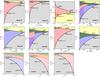 |
Fig. 1 Mass distribution of the three components H/He (yellow), water, and rocks (gray) for the 11 series A − K described in Table 1. Each panel shows various models running vertically, which differ in transition pressure P1 − 2 in the case of 3L models, and in envelope water mass fraction Z1 for 2L models (series C, F, and I). Thick black lines show layer boundaries, and numbers close to filled black circles denote temperature in K and pressure in Mbar. Water is subdivided into five colors coding fluid molecular and fluid dissociated water (green), plasma (red), superionic water (blue), an undissolved region in the water phase diagram close to the superionic phase (violet), and fluid dissociated water (orange) in series C, F, and G. In series C, F and I, the H/He mass fraction can be obtained via (1 − Z1) × (1 − Mcore/Mp). In series G, the center of the planet is at the top of the figure while for all other series, the center is at the bottom. |
In series H, we see agreement only if P1 − 2 ≈ 80 GPa.
However, the water shell is in the plasma phase, so that strict separation from the H/He
envelope might not be realized. We conclude that models of series H are unlikely. The same
argument holds for series A, D, and G. With series C and F, strict and relaxed conditions
give the same possible range of models. We see agreement, if
Z1 ≈ 0.6 (F: 0.4 − 0.5), while the H/He content becomes too
large for higher envelope metallicities, and the total water mass fraction too small for
lower metallicities. Models of series C are cold enough for water to be superionic.
Whether a lattice structure of the oxygen subsystem or homogeneity throughout such an
envelope can be maintained remains to be investigated. With series I, we see agreement if
Z1 = 0.55 − 0.7. These models have
Tcore ≈ 13300 K and
Pcore = 3 − 5.3 Mbar, where water is in a plasma state, hence
likely to be mixed with the H/He component. The same holds for the allowed series F
models, where Tcore = 8100 − 8500 K. Thus these models can be
considered self-consistently. With series J, we see agreement if
P1 − 2 = 65 − 110 Mbar, where water close to the core is
superionic justifying the assumption of a water shell. The fluid fraction of the water
layer might be mixed into the H/He envelope. The same holds for series E
( ), which
differs from series J (
), which
differs from series J ( ) only in mean
mass density
) only in mean
mass density  .
The similarity of the range of series E and J models implies that the upper limit of this
observational quantity is sufficiently well known.
.
The similarity of the range of series E and J models implies that the upper limit of this
observational quantity is sufficiently well known.
For series K models, the H/He content is clearly more than predicted by Figueira et al. (2009), since they investigate the
formation of a planet with
Rp ≤ 4.4R⊕, whereas in
series K, Rp = 5.35R⊕
( ), requiring a
larger fraction of light elements. However, Lecavelier des Etangs (2007) predicts complete evaporation of GJ436b within
5 Ga, if
), requiring a
larger fraction of light elements. However, Lecavelier des Etangs (2007) predicts complete evaporation of GJ436b within
5 Ga, if  . While
contrary positions exist (Erkaev et al. 2007),
theoretical mass loss rates offer a way to tighten the uncertainty in age and maximal
radius of GJ436b.
. While
contrary positions exist (Erkaev et al. 2007),
theoretical mass loss rates offer a way to tighten the uncertainty in age and maximal
radius of GJ436b.
According to the models by Spiegel et al. (2010), the atmosphere is isothermal at T = 1300 K between about 1 and 100 − 1000 bar, corresponding to our series H and I. From the discussion above, inconsistency with the water phase diagram of series H indicates that water is at least partially mixed within the H/He envelope. The extreme case of complete mixing between H/He and H2O is realized in series I. Models of that series with Z1 = 0.55 − 0.70 give the best overall agreement with available constraints. Those models have an H/He mass fraction of 0.13 − 0.145, while core mass and water mass fraction cover the range proposed by Figueira et al. (2009). Alternative constraints may become available from improved formation models and atmosphere models in the future and be applied to our broad set of series so that improved estimates of the bulk composition can then be derived from Fig. 1.
Our models comprise those by Rogers & Seager (2010a), who find an H/He mass fraction of 2 − 14.5%. Temperature-effects of our water equation of state tend to enhance the volume of a mass shell at given pressure level, requiring less H/He to be added to reproduce the large radius. At typical internal conditions P ~ 2 Mbar and T ~ 6000 K in GJ436b, the temperature effects enhance the volume by ≈ 20% compared to water at 300 K (French et al. 2009). For this reason, we are able to find models with very low H/He mass fractions ( ≈ 10-3 Mp).
3.2. Love number, core mass, and metallicity of GJ 436b
For various models we calculated the Love number k2. This parameter is known to measure the central condensation or, equivalently, homogeneity of matter in a nearly spherical object (Zharkov & Trubitsyn 1978) with an upper limit of 3/2 for a sphere of constant density and a lower limit of zero for Roche-type models. Jupiter’s theoretical value is k2,J ~ 0.49 (Ragozzine & Wolf 2009) indicating a close to n = 1 polytropic density profile, which is confirmed by our calculations. For Neptune, we find k2,N = 0.16 indicating stronger central condensation, for Saturn we find intermediate values around k2,S = 0.32, and for an artificial Mp = 20M⊕ water planet we find k2,W = 0.89, in agreement with water being less compressible than the H/He dominated envelopes of the solar giant planets. Finally for GJ436b, we find k2 ranging from 0.02 to 0.82. These results are displayed in Fig. 2, together with the uncertainty in core mass of these planets.
Models of GJ436b with k2 = 0.02 − 0.2 are accompanied by any core mass between 0 and ≈ 0.9 Mp: a measurement of k2 in this regime would not help to constrain the interior any further. All our calculated 3L models with metal-free or low-metallicity H/He envelopes fall into this degenerate regime. Beyond the region of strong degeneracy at k2 > 0.2, the uncertainty in Mcore for an observationally given k2 shrinks with k2, so that upper limits for the uncertainty in core mass can be derived, if k2 and the atmospheric temperature profile are known. Those models are necessarily two-layer models with one homogeneous envelope. Assuming for instance an atmospheric temperature of 1300 K, then any redistribution of metals from the outer part of the envelope to the inner part of the envelope would (if the central condensation is to be kept at constant k2 value) require a compensating transport of matter from the core upward, making the core mass decrease and drop below the upper limit for that atmospheric temperature at any given k2. This upper limit in core mass increases with decreasing atmospheric temperature, since dense envelopes act to reduce the density gap between envelope and core, which would reduce the central cendensation (k2), if it was not compensated for by a more massive core. If we adopt 300 K as coldest possible temperature of an isothermal atmosphere, then the area above the blue dashed curve in Fig. 2 is not accessible by present GJ436b. The high-core mass end of that curve corresponds to a zero-metallicity envelope. At the high-core mass end, however, the solutions lie in the area of large degeneracy, where besides the mass the mean density of the core strongly affects k2, and the behavior of solutions is no longer a simple function of envelope metallicity and temperature.
At Saturn’s theoretical k2,S = 0.32, the uncertainty in core mass is ≈0.4 Mp, it is ≈0.2 Mp at Jupiter’s k2,J = 0.49, and it is ≤ 0.15 Mp for k2 > 0.6. Such high k2 values, if measured, imply high outer envelope metallicities for this planet. For 2L models, we find 0.55 < Z1 < 0.78 in 300 K cold atmospheres, and 0.7 < Z1 < 0.884 in 1300 K hot atmospheres, where k2 is a sensitive function of Z1. An observational k2 value between 0.3 and 0.8 would help constrain envelope metallicity and core mass.
Furthermore, a superionic water layer can be regarded in the traditional manner as a former ice layer of the initial core that warmed up during formation through mass accretion and contraction. Adding the mass of the water layer to the underlying rocky core results in significantly higher core masses. The case of Neptune illustrates the general difficulty of applying the label core mass to metal-rich planets with a layered structure.
3.3. M–R relations for water planets
Figure 3 shows
M − R relations of water-planets with a small
(0.25M⊕) rocky core, using H2O-REOS. We present
the M − R relation for profiles with an isothermal
atmosphere down to 1 kbar of 1000 K, 2000 K, for fully adiabatic profiles starting with
T1 = 1000 K, and, for comparison, for the fit-formula from
Fortney et al. (2007b) for pure adiabatic water
planets based on a finite temperature correction to a zero-K isotherm of water. Our
M − R relations for
T1 = 1000 K can be fitted with the formula  (1)with
a0 = 1.6586, a1 = 0.9950,
a2 = 0.1549, a3 = 0 for the
solid line and a0 = 2.8210,
a1 = − 0.2928, a2 = 0.9037,
a3 = − 0.1760 for the dashed-dot line in Fig. 3. This uncertainty in the atmospheric temperature
profile (isothermal or adiabatic) obviously influences the radius
by ~ 0.5R⊕.
(1)with
a0 = 1.6586, a1 = 0.9950,
a2 = 0.1549, a3 = 0 for the
solid line and a0 = 2.8210,
a1 = − 0.2928, a2 = 0.9037,
a3 = − 0.1760 for the dashed-dot line in Fig. 3. This uncertainty in the atmospheric temperature
profile (isothermal or adiabatic) obviously influences the radius
by ~ 0.5R⊕.
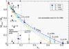 |
Fig. 2 Love number k2 and core mass of two-layer models (squares connected by dashed lines), three-layer models with metal-free envelopes (triangles), and three-layer models with low-metallicity envelopes (diamonds) of GJ 436b. Color-coded circles are for interior models of Jupiter (red), Saturn (yellow), and Neptune (blue), and a 20M⊕ water planet (black). Adding the mass of the water layer to the mass of the rocky core shifts 3L models solutions from filled to open triangles, and the Neptune model to the position as indicated by an arrow. For each of the dashed lines (which are for different isothermal atmospheres of 300 K (blue), 700 K (cyan), and 1300 K (orange)), the squares indicate solutions for Z1 = 0, 0.5, and the highest possible value when Mcore = 0. On the left hand side of the gray dashed line at k2 = 0.2, the models are highly degenerate, and on the right hand side, no metal-free envelope models were found. |
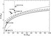 |
Fig. 3 Mass-radius relationships of water planets in comparison with Uranus (U), Neptune (N), the three known Neptune-mass planets, and the two known super-Earth mass planets GJ1214b and CoRoT-7b. Solid line: T1 = 1000 K, isothermal atmosphere, Mcore = 0.25 M⊕; dashed line: same as solid line but T1 = 2000 K; dot-dashed line: same as solid line but adiabatic atmosphere; thin solid line: fit-formula for water planets from Fortney et al. (2007b). The thin dashed-dot line is the theoretical M − R relation for Mg-silicate planets from Valencia et al. (2010). |
In the 5 − 50 M⊕ planet mass region, previous and current M − R relations are similar with a flatter radius dependence in the latter case indicating a smaller polytropic exponent γ. In particular, the interior profiles of our water planets can be approximated well by γ = 2.8 for 2 < ρ < 4 g cm-3 and γ = 2.4 for ρ > 4 g cm-3. The resulting theoretical radii of water planets are below the observed radius of the three currently known Neptune-mass planets GJ436b, HAT-P-11b (Bakos et al. 2010), and Kepler-4b (Borucki et al. 2010), indicating the presence of low-Z material in these planets. In case of warm atmospheric temperatures of 1000 K or more, an outer H/He envelope that contributes in radius ~ 15% may contribute ≪ 1% in mass. The only known planet whose observational parameters Mp, Rp, and Teq can be explained by the assumption of a water-dominated water+rock composion without H/He (Rogers & Seager 2010b) is GJ1214b, whereas for the super-Earth CoRoT-7b (Leger et al. 2009), Mp = 4.8 ± 0.8, a water mass fraction < 10% and an H/He mass fraction < 0.01% are predicted by evolution calculations that include the energy-limited mass loss caused by stellar irradiation (Valencia et al. 2010).
4. Discussion
4.1. A secondary planet
To explain the high eccentricity e = 0.15 of GJ436b, the presence of a secondary planet has been suggested (Ribas et al. 2008) but not yet confirmed by measurements (Bean et al. 2008). While observations exclude a resonant perturber in 2:1 resonance down to lunar mass, the presence of a secular perturber at distant orbit in apsidal alingment with GJ436b is still an appealing possibility (Batygin et al. 2009a). If detected, the scheme presented in Batygin et al. (2009b) allows determination of k2, if the planets are on coplanar orbits (Mardling 2010). We predict 0.02 ≤ k2 < 0.82.
If future measurements deny there is a secular perturber, a (minimum) Love number can be
estimated by requiring sufficiently weak tidal interactions between planet and star that
would allow for the planet’s presence at observed orbital distance and eccentricity. Using
the common low-eccentricity approximation of the tidal evolution equations, Jackson et al. (2008) find that an effective constant
tidal Q′ value of 106.5 results in an initial
a0 − e0 distribution that best
matches the observed distribution of tidally unevolved planets. With
Q′ = 3Qp / 2k2
(in the approximation of incompressible homogeneous matter; see Goldreich & Soter 1966; Love
1911, Sect. 123) where  is the
tidal dissipation function, and with
Qp = QN = (0.9 − 33) × 104
(Zhang & Hamilton 2008; Banfield & Murray 1992) as proposed for Neptune,
this implies k2 = 0.0043 − 0.156. We find
k2 ≥ 0.02. This raises the possibility that the
Q value of GJ436b is close to Neptune’s upper limit, making the
eccentricity a consequence of weak tidal interaction with the star.
is the
tidal dissipation function, and with
Qp = QN = (0.9 − 33) × 104
(Zhang & Hamilton 2008; Banfield & Murray 1992) as proposed for Neptune,
this implies k2 = 0.0043 − 0.156. We find
k2 ≥ 0.02. This raises the possibility that the
Q value of GJ436b is close to Neptune’s upper limit, making the
eccentricity a consequence of weak tidal interaction with the star.
However, according to Jackson et al. (2008) the initial eccentricity of GJ436b would have been e0 ≈ 0.6, which has been demonstrated to lie beyond the range of applicability of the low-eccentricity approximation, as the theoretical tidal evolution timescale can decrease by several orders of magnitude when the exact orbital evolution theory is used (Leconte et al. 2010). A re-calculation of GJ436b’s tidal evolution would therefore be helpful in order to obtain present-time (Q′,k2) pairs that reproduce the observed orbital parameters, thereby clarifying the need for an external perturbing body.
4.2. Constraints from formation and atmosphere profiles
Among the broad sets of models presented here, those that are consistent with available constraints from formation theory, model atmospheres, and solubility of fluid water in H/He have a warm outer envelope with water mass fraction 55 − 70%, and a rocky core. At such large envelope heavy element abundances, k2 begins to be sensitive to core mass. On the other hand, measuring k2 > 0.3 would either imply a violation of the condition from formation theory Mrock/Mp > 0.45 or indicate the presence of rocks in the envelopes (partially replacing water). In the outer part of the envelope, water is in a supercritical fluid state and then transits to the plasma phase because of rising temperatures. This supports the assumption that water is mixed into the H/He envelope in the two layer models instead of forming a separate layer as in the three layer models. Depending on the process of formation, however, a separation into few distinct layers with different water fractions can be possible. Colder models where water is in a superionic state at 3000 − 6000 K are not consistent with the ≈ 1300 K hot model atmospheres by Spiegel et al. (2010) or the recent model atmospheres by Lewis et al. (2010) which predict a radiative layer between 1 and 100 bar at 1100 to 1200 K depending on metallicity. High-pressure ice phases occur at even lower temperatures, hence in none of our models. Considering water as a proxy for metals, higher H/He mass fractions are possible than the 0.13 − 0.145 of the preferred models. The broad set of models presented here demonstrates the importance of accurate model atmospheres. Neglecting the available constraints from formation and atmosphere models, the set of solutions satisfying only Mp, Rp and consistency with Tp,eff includes models with MH / He/Mp = 10-3 and MH2O / Mp = 0.999.
4.3. Constraints from atmosphere observations
For GJ436b, an observational value k2 > 0.5 implies a rocky core mass below 0.2 Mp and an envelope metallicity over 50%. An observational value k2 > 0.2 would imply Mcore < 0.55 Mp, and Z1 above ≈40% if the envelope is homogeneous. While homogeneous envelope models are supported by the hot internal temperatures and miscibility of water and hydrogen, we cannot be sure about the absence of envelope layer boundaries, so can only obtain upper limits for the core mass for any given k2 value. In order to break this degeneracy further, an estimate of the outer envelope metallicity is required.
For solar system giant planets, atmospheric heavy element abundances are only known within a factor of a few for some species that do not condense at optically thick deeper levels. The abundances are believed to be representative of the outer envelope because of vertical mixing still at high altitudes below 1 bar. Irradiated extrasolar planets, such as GJ 436b however, become optically thick at pressures several orders of magnitude lower than the onset of the convective envelope. Even in the fortunate case of measured atmospheric abundances, representative metallicity determinations might require including non-equilibrium chemistry, cloud formation, vertical mixing beyond mixing-length theory, and other effects. On the other hand, current theoretical and observational progress is encouraging. Transmission and emission spectra predicted by state-of-the-art model atmospheres exhibit various observational signatures in dependence on metallicity. Chabrier et al. (2007) found a 30% decrease of a hot Jupiter’s emission at 4.5 μm due to encanced absorption by CO when the overall metallicity was enhanced from 1 × to 5 × solar. For super-Earth atmospheres, Miller-Ricci et al. (2009) found large hydrogen fractions (low mean molecular weight) to map on a detectable variability of the transit radius with wavelength and a rapid decrease in variability with mean molecular weight. For GJ436b in particular, Lewis et al. (2010) developed a three-dimensional atmospheric circulation model and predict metal-enhanced atmospheres to reveal themselves in an orbital phase dependency of spectra potentially detectable during future missions. In addition, secondary eclipse measurements (Stevenson et al. 2010) already provide hints of a strongly (30 − 50 × solar) metal-enhanced atmosphere (Lewis et al. 2010).
4.4. Comparison with Uranus and Neptune
Interior models of Uranus (Mp = 14.5M⊕) predict that at least 21% by mass is H/He, and at least 15% in Neptune (Mp = 17.1M⊕) (Fortney & Nettelmann 2010). This is consistent with the preferred model values for GJ 436b (13 − 14.5%) considering that some fraction of water as assumed in the model calculations could indeed be rocks and H/He in the envelope of either of the planets. On the other hand, since only lower limits of the H/He to ice and rock ratios in these planets can be derived, their composition can also be very different from each other. Irradiation by the close-by parent star may rise the core temperatures of preferred GJ436b models significantly above those of Uranus and Neptune, where adiabatic models predict Tcore = 6000 − 7000 K, hence water in the superionic phase. Methane has been suggested as separating into metallic hydrogen and diamond (e.g. Hirai et al. 2009) at those deep interior conditions, so that the interior of those planets might be organized very different by that from GJ436b, even in the case of similar bulk composition. Interior models of Uranus and Neptune require supersolar heavy element abundance in the outer envelope and some admixture of H/He in the deep interior, which can be represented by at least two envelopes with different compositions. Such a structure is bracketed by our 2L and 3L models. The observed low heat flux of Uranus and, to a lesser extend, of Neptune gives further evidence of layer boudaries, or more general, inhomogeneities in these planets (Hubbard et al. 1995). Unfortunately, the age of GJ436 is poorly known, but investigations of the cooling behavior of various interior models can help further rule out or strenghten some of the models presented here.
4.5. Conclusions
Applying H-, He-, and H2O-REOS for hydrogen, helium, and water to generate three-layer models (H/He envelope, water envelope, rocky core) and two-layer models (H/He/H2O envelope, rocky core) of GJ 436b, we find interior models ranging from large rocky cores with significant H/He layers to almost pure water worlds with thin, but extended H/He atmospheres. If water occurs and the 1 kbar temperature is not much higher than 700 K, this exoplanet constitutes the third natural potential object for realyzing superionic water, besides the deep interior of Uranus and Neptune. In the H/He envelope, the temperature rises rapidly such that we do not find high-pressure ice phases in the inner envelope. Indeed, if we assume temperature profiles in good agreement with model atmospheres, water in the interior of GJ436b transits from fluid to plasma, favoring an outer envolope with strong water enrichment instead of a separation into two distinct envelopes.
The Love number k2 of different possible compositions with metal-free outer H/He envelopes varies from 0.02 to 0.2. In this k2 regime, the core mass depends non-uniquely on k2 and cannot be derived from a measurement of k2. An observationally derived value k2 > 0.2 (0.3; 0.5) would imply Mcore < 0.55 Mp (Mcore < 0.4 Mp; Mcore < 0.2 Mp) and a high outer envelope metallicity.
The radius of GJ436b is larger than predicted for warm-water planets. Even in case of the warmest models found, a small H/He fraction of 10-3 Mp is necessary to account for the radius. Calculating the cooling behavior on the basis of a proper treatment of the atmosphere might help to better constrain the interior of this planet.
With this work we want to motivate both accurate transit-timing observations of this planet that aim to clarify the existence of a secondary planet and that may allow derivation of k2 and transmission spectra measurements aimed at determining the atmospheric metallicity.
Acknowledgments
We acknowledge discussions with P.H. Hauschildt, M. French, and J.J. Fortney and are grateful to D.J. Stevenson for his introduction to Love numbers and mentorship to one of us (UK). We thank the anonymous referee for his comments which extraordinarily helped to reshape and improve the paper. This work was supported by the DFG within the SFB 652 and the grant RE 882/11-1 and by the HLRN within the grants mvp00001 and mvp00006. We thank the Rechenzentrum of the U Rostock for assistance. R.N. acknowledges general support from the German National Science Foundation (Deutsche Forschungsgemeinschaft, DFG) in grants NE 515/13-1, 13-2, and 23-1, as well as support from the EU in the FP6 MC ToK project MTKD-CT-2006-042514.
References
- Adams, E. R., Seager, S., & Elkins-Tanton, L. 2008, ApJ, 673, 1160 [NASA ADS] [CrossRef] [Google Scholar]
- Bakos, G. A., Torres, G., Pál, A., et al. 2010, ApJ, 710, 1724 [NASA ADS] [CrossRef] [Google Scholar]
- Banfield, D., & Murray, N. 1992, Icarus, 99, 390 [NASA ADS] [CrossRef] [Google Scholar]
- Baraffe, I., Chabrier, G., & Barman, T. 2008, A&A, 482, 315 [NASA ADS] [CrossRef] [EDP Sciences] [Google Scholar]
- Batygin, K., Bodenheimer, P., & Laughlin, G. 2009b, ApJ, 704, L49 [NASA ADS] [CrossRef] [Google Scholar]
- Batygin, K., Laughlin, G., Meschiari, S., et al. 2009a, ApJ, 699, 23 [NASA ADS] [CrossRef] [Google Scholar]
- Bean, J. L., Benedict, G. F., & Endl, M. 2006, ApJ, 653, L65 [NASA ADS] [CrossRef] [Google Scholar]
- Bean, J. L., Benedict, G. F., Charbonneau, D., et al. 2008, A&A, 468, 1039 [NASA ADS] [CrossRef] [EDP Sciences] [Google Scholar]
- Borucki, W. J., Koch, D., Basri, G., et al. 2010, Science, 327, 977 [NASA ADS] [CrossRef] [PubMed] [Google Scholar]
- Burrows, A., Budaj, J., & Hubeny, I. 2008, ApJ, 678, 1436 [NASA ADS] [CrossRef] [Google Scholar]
- Butler, R. P., Vogt, S. S., Marcy, G. W., et al. 2004, ApJ, 617, 580 [NASA ADS] [CrossRef] [Google Scholar]
- Chabrier, G., Baraffe, I., Selsis, F., et al. 2007, in Protostars and Planets V, ed. B. Reipurth, D. Jewitt, & K. Keil (University of Arizona Press and LPI), 623 [Google Scholar]
- Charbonneau, D., Zachory, B. K., Irwin, J., et al. 2009, Nature, 462, 891 [NASA ADS] [CrossRef] [PubMed] [Google Scholar]
- Coughlin, J., Stringfellow, G., Becker, A., et al. 2008, ApJ, 689, L149 [Google Scholar]
- Deming, D., Harrington, J., Laughlin, G., et al. 2007, ApJ, 667, L199 [NASA ADS] [CrossRef] [Google Scholar]
- Demory, B.-O., Gillon, M., Barman, T., et al. 2007, A&A, 475, 1125 [NASA ADS] [CrossRef] [EDP Sciences] [Google Scholar]
- Erkaev, N. V., Kulikov, Y. N., Lammer, H., et al. 2007, A&A, 472, 329 [NASA ADS] [CrossRef] [EDP Sciences] [Google Scholar]
- Figueira, P., Pont, F., Mordasini, C., et al. 2009, A&A, 493, 671 [NASA ADS] [CrossRef] [EDP Sciences] [Google Scholar]
- Fortney, J. J., & Nettelmann, N. 2010, Springer Space Sci. Rev., 157, 423 [CrossRef] [Google Scholar]
- Fortney, J. J., Marley, M. S., & Barnes, J. W. 2007a, ApJ, 659, 1661 [NASA ADS] [CrossRef] [Google Scholar]
- Fortney, J. J., Marley, M. S., & Barnes, J. W. 2007b, ApJ, 668, 1267 [NASA ADS] [CrossRef] [Google Scholar]
- French, M., Mattsson, T. R., Nettelmann, N., & Redmer, R. 2009, Phys. Rev. B, 79, 954107 [Google Scholar]
- Gautier, D., Conrath, B. J., Owen, T., de Pater, I., & Atreya, S. K. 1995, in Neptune and Triton, ed. Cruishank (Tucson: University of Arizona), 547 [Google Scholar]
- Gillon, M., Demory, B.-O., Barman, T., et al. 2007a, A&A, 471, L51 [NASA ADS] [CrossRef] [EDP Sciences] [Google Scholar]
- Gillon, M., Pont, F., Demory, B.-O., et al. 2007b, A&A, 472, L13 [NASA ADS] [CrossRef] [EDP Sciences] [Google Scholar]
- Goldreich, P., & Soter, S. 1966, Icarus, 5, 375 [NASA ADS] [CrossRef] [Google Scholar]
- Guillot, T., Chabrier, G., Morel, P., & Gautier, D. 1994, Icarus, 112, 354 [NASA ADS] [CrossRef] [Google Scholar]
- Hirai, H., Konagai, K., Kawamura, T., Yamamoto, Y., & Yagi, T. 2009, Physics of the Earth and Planetary Interiors, 174, 242 [NASA ADS] [CrossRef] [Google Scholar]
- Holst, B., Redmer, R., & Desjarlais, M. P. 2008, Phys. Rev. B, 77, 184201 [NASA ADS] [CrossRef] [Google Scholar]
- Hubbard, W. B. 1984, Planetary Interiors (Van Nostrand Reinhold Company Inc.) [Google Scholar]
- Hubbard, W. B., & MacFarlane, J. J. 1980, J. Geophys. Res., 88, 225 [NASA ADS] [CrossRef] [Google Scholar]
- Hubbard, W. B., & Marley, M. S. 1989, Icarus, 78, 102 [NASA ADS] [CrossRef] [Google Scholar]
- Hubbard, W. B., Podolak, M., & Stevenson, D. J. 1995, in Neptune and Triton, ed. Cruishank (Tucson: University of Arizona), 109 [Google Scholar]
- Jackson, B., Greenberg, R., & Barnes, R. 2008, ApJ, 678, 1396 [NASA ADS] [CrossRef] [Google Scholar]
- Kenyon, S. J., & Hartman, L. 1995, ApJS, 101, 117 [NASA ADS] [CrossRef] [Google Scholar]
- Kietzmann, A., Holst, B., Redmer, R., Desjarlais, M. P., & Mattsson, T. R. 2007, Phys. Rev. Lett., 98, 190602 [NASA ADS] [CrossRef] [PubMed] [Google Scholar]
- Lecavelier des Etangs, A. 2007, A&A, 461, 1185 [NASA ADS] [CrossRef] [EDP Sciences] [Google Scholar]
- Leconte, J., Chabrier, G., Baraffe, I., & Levrard, B. 2010, A&A, 516, A64 [NASA ADS] [CrossRef] [EDP Sciences] [Google Scholar]
- Leger, A., Rouan, D., Schneider, R., et al. 2009, A&A, 506, L287 [CrossRef] [EDP Sciences] [Google Scholar]
- Lewis, N. K., Showman, A. P., Fortney, J. J., et al. 2010, ApJ, 720, L344 [NASA ADS] [CrossRef] [Google Scholar]
- Love, A. E. H. 1911, Some problems of geodynamics (Cambridge University Press) [Google Scholar]
- Lyon, S., & Johnson, J. D. E. 1992, SESAME: Los Alamos National Laboratory Equation of State Database, Tech. rep., LANL report no. LA-UR-92-3407 [Google Scholar]
- Maness, H. L., Marcy, G. W., Ford, E. B., et al. 2007, PASP, 119, 90 [NASA ADS] [CrossRef] [Google Scholar]
- Mardling, R. A. 2010, MNRAS, accepted [Google Scholar]
- Miller-Ricci, E., Seager, S., & Sasselov, D. 2009, ApJ, 690, 1056 [NASA ADS] [CrossRef] [Google Scholar]
- Nettelmann, N., Holst, B., Kietzmann, A., et al. 2008, ApJ, 683, 1217 [NASA ADS] [CrossRef] [Google Scholar]
- Podolak, M., Podolak, J. I., & Marley, M. S. 2000, Planet. Space Sci., 48, 143 [NASA ADS] [CrossRef] [Google Scholar]
- Ragozzine, D., & Wolf, A. S. 2009, ApJ, 698, 1778 [NASA ADS] [CrossRef] [Google Scholar]
- Redmer, R., Mattsson, T. R., Nettelmann, N., & French, M. 2010, Icarus, accepted [Google Scholar]
- Ribas, I., Font-Ribera, A., & Beaulieu, J.-P. 2008, ApJ, 677, L59 [NASA ADS] [CrossRef] [MathSciNet] [Google Scholar]
- Rogers, L. A., & Seager, S. 2010a, ApJ, 712, 974 [NASA ADS] [CrossRef] [Google Scholar]
- Rogers, L. A., & Seager, S. 2010b, ApJ, 716, 1208 [NASA ADS] [CrossRef] [Google Scholar]
- Seager, S., Kuchner, M., Hier-Majumder, A., & Militzer, B. 2007, ApJ, 669, 1279 [NASA ADS] [CrossRef] [Google Scholar]
- Spiegel, D. S., Burrows, A., Ibgui, L., Hubeny, I., & Milsom, J. A. 2010, ApJ, 709, 149 [NASA ADS] [CrossRef] [Google Scholar]
- Stevenson, D. J. 1982, Ann. Rev. Earth Sci., 10, 257 [Google Scholar]
- Stevenson, K. B., Harrington, J., Nymeyer, S., et al. 2010, Nature, 464, 1161 [NASA ADS] [CrossRef] [PubMed] [Google Scholar]
- Torres, G., Winn, J. N., & Holman, M. J. 2008, ApJ, 677, 1324 [NASA ADS] [CrossRef] [Google Scholar]
- Valencia, D., Ikoma, M., Guillot, T., & Nettelmann, N. 2010, A&A, 516, A20 [NASA ADS] [CrossRef] [EDP Sciences] [Google Scholar]
- Zhang, K., & Hamilton, D. P. 2008, Icarus, 193, 267 [NASA ADS] [CrossRef] [Google Scholar]
- Zharkov, V. N., & Trubitsyn, V. P. 1978, Physics of Planetary Interiors (Tucson: Parchart) [Google Scholar]
All Tables
All Figures
|
Fig. 1 Mass distribution of the three components H/He (yellow), water, and rocks (gray) for the 11 series A − K described in Table 1. Each panel shows various models running vertically, which differ in transition pressure P1 − 2 in the case of 3L models, and in envelope water mass fraction Z1 for 2L models (series C, F, and I). Thick black lines show layer boundaries, and numbers close to filled black circles denote temperature in K and pressure in Mbar. Water is subdivided into five colors coding fluid molecular and fluid dissociated water (green), plasma (red), superionic water (blue), an undissolved region in the water phase diagram close to the superionic phase (violet), and fluid dissociated water (orange) in series C, F, and G. In series C, F and I, the H/He mass fraction can be obtained via (1 − Z1) × (1 − Mcore/Mp). In series G, the center of the planet is at the top of the figure while for all other series, the center is at the bottom. |
| In the text | |
|
Fig. 2 Love number k2 and core mass of two-layer models (squares connected by dashed lines), three-layer models with metal-free envelopes (triangles), and three-layer models with low-metallicity envelopes (diamonds) of GJ 436b. Color-coded circles are for interior models of Jupiter (red), Saturn (yellow), and Neptune (blue), and a 20M⊕ water planet (black). Adding the mass of the water layer to the mass of the rocky core shifts 3L models solutions from filled to open triangles, and the Neptune model to the position as indicated by an arrow. For each of the dashed lines (which are for different isothermal atmospheres of 300 K (blue), 700 K (cyan), and 1300 K (orange)), the squares indicate solutions for Z1 = 0, 0.5, and the highest possible value when Mcore = 0. On the left hand side of the gray dashed line at k2 = 0.2, the models are highly degenerate, and on the right hand side, no metal-free envelope models were found. |
| In the text | |
|
Fig. 3 Mass-radius relationships of water planets in comparison with Uranus (U), Neptune (N), the three known Neptune-mass planets, and the two known super-Earth mass planets GJ1214b and CoRoT-7b. Solid line: T1 = 1000 K, isothermal atmosphere, Mcore = 0.25 M⊕; dashed line: same as solid line but T1 = 2000 K; dot-dashed line: same as solid line but adiabatic atmosphere; thin solid line: fit-formula for water planets from Fortney et al. (2007b). The thin dashed-dot line is the theoretical M − R relation for Mg-silicate planets from Valencia et al. (2010). |
| In the text | |
Current usage metrics show cumulative count of Article Views (full-text article views including HTML views, PDF and ePub downloads, according to the available data) and Abstracts Views on Vision4Press platform.
Data correspond to usage on the plateform after 2015. The current usage metrics is available 48-96 hours after online publication and is updated daily on week days.
Initial download of the metrics may take a while.