| Issue |
A&A
Volume 522, November 2010
|
|
|---|---|---|
| Article Number | A92 | |
| Number of page(s) | 19 | |
| Section | Cosmology (including clusters of galaxies) | |
| DOI | https://doi.org/10.1051/0004-6361/201015165 | |
| Published online | 05 November 2010 | |
The Sloan great wall. Rich clusters
1
Tartu Observatory,
61602
Tõravere,
Estonia
e-mail: This email address is being protected from spambots. You need JavaScript enabled to view it.
2
Tuorla Observatory, University of Turku,
Väisäläntie 20,
Piikkiö,
Finland
3
Finnish Centre of Astronomy with ESO (FINCA), University of Turku,
Väisäläntie 20,
Piikkiö,
Finland
4
Institute of Physics, Tartu University,
Tähe 4,
51010
Tartu,
Estonia
5
Observatori Astronòmic, Universitat de València,
Apartat de Correus
22085, 46071
València,
Spain
Received:
7
June
2010
Accepted:
8
July
2010
Abstract
Aims. We present the results of the study of the substructure and galaxy content of ten rich clusters of galaxies in three different superclusters of the Sloan great wall, the richest nearby system of galaxies (hereafter SGW).
Methods. We determine the substructure in clusters using the “Mclust” package from the “R” statistical environment and analyse their galaxy content with information about colours and morphological types of galaxies. We analyse the distribution of the peculiar velocities of galaxies in clusters and calculate the peculiar velocity of the first ranked galaxy.
Results. We show that five clusters in our sample have more than one component; in some clusters the different components also have different galaxy content. In other clusters there are distinct components in the distribution of the peculiar velocities of galaxies. We find that in some clusters with substructure the peculiar velocities of the first ranked galaxies are high. All clusters in our sample host luminous red galaxies; in eight clusters their number exceeds ten. Luminous red galaxies can be found both in the central areas of clusters and in the outskirts, some of them have high peculiar velocities. About 1/3 of the red galaxies in clusters are spirals. The scatter of colours of red ellipticals is in most clusters larger than that of red spirals. The fraction of red galaxies in rich clusters in the cores of the richest superclusters is larger than the fraction of red galaxies in other very rich clusters in the SGW.
Conclusions. The presence of substructure in rich clusters, signs of possible mergers and infall, and the high peculiar velocities of the first ranked galaxies suggest that the clusters in our sample are not yet virialized. We present merger trees of dark matter haloes in an N-body simulation to demonstrate the formation of present-day dark matter haloes via multiple mergers during their evolution. In simulated dark matter haloes we find a substructure similar to that in observed clusters.
Key words: large-scale structure of the Universe / galaxies: clusters: general
© ESO, 2010
1. Introduction
Most galaxies in the Universe are located in groups and clusters of galaxies, which in turn reside in larger systems – in superclusters of galaxies or in filaments crossing underdense regions between superclusters. According to the Cold Dark Matter model, groups and clusters of galaxies form hierarchically through the merging of smaller systems (Loeb 2009; Knebe & Müller 2000, and references therein). The timescale of the evolution of groups depends on their global environment (Tempel et al. 2009). As a result, the properties of groups depend on the environment where they are embedded, richer and more luminous groups are located in a higher-density environment than poor, less luminous groups (Einasto et al. 2003a,b, 2005; Berlind et al. 2006). An understanding of the properties and evolutionary state of groups and clusters of galaxies in different environments, and of the properties of galaxies in them is important for the study of groups and clusters, as well as for the study of the properties and evolution of galaxies and larger structures – superclusters of galaxies.
Detailed knowledge of properties of clusters of galaxies is also needed for comparison of observations with N-body calculations of the formation and evolution of cosmic structures.
Galaxies and galaxy systems form because of initial density perturbations of different scales. Perturbations of a scale of about 100 h-1 Mpc1 give rise to the largest superclusters. The largest and richest superclusters, which may contain several tens of rich (Abell) clusters, are the largest coherent systems in the Universe with characteristic dimensions of up to 100 h-1 Mpc. At large scales a dynamical evolution takes place at a slower rate, and the richest superclusters have retained the memory of the initial conditions of their formation, and of the early evolution of structure (Kofman et al. 1987). Rich superclusters have high density cores that are absent in poor superclusters (Einasto et al. 2007b). The core regions of the richest superclusters may contain merging X-ray clusters (Rose et al. 2002; Bardelli et al. 2000; Belsole et al. 2004). The formation of rich superclusters had to begin earlier than that of the smaller structures; they are the sites of early star and galaxy formation (e.g. Mobasher et al. 2005), and the first places where systems of galaxies form (e.g. Venemans et al. 2004; Ouchi et al. 2005).
Among the richest galaxy systems, the Sloan Great Wall, which is the richest system of galaxies in the nearby Universe (Vogeley et al. 2004; Gott et al. 2005; Nichol et al. 2006), deserves special attention. The SGW consists of several rich and poor superclusters connected by lower density filaments of galaxies, representing a variety of global environments from the high density core of the richest supercluster in the SGW to a lower density poor supercluster at the edge of the SGW. The superclusters in the SGW differ in morphology and galaxy content, which suggests that their formation and evolution has been different (Einasto et al. 2010, in prep., hereafter E10).
Our aim in the present paper is to study the properties of the richest clusters of galaxies in the SGW. Our clusters come from all the superclusters in the SGW so that we can compare the dynamical state and galaxy content of the richest clusters in different environments, from the high-density core of the richest supercluster to clusters in a poor supercluster in the extension of the SGW.
The present-day dynamical state of clusters of galaxies depends on their formation history. One indicator of the former or ongoing mergers between groups and clusters is the presence of substructure in clusters (Knebe & Müller 2000, and references therein). The substructure affects the estimates of several cluster characteristics, the dynamical mass and mass-to-light ratio among others (see Biviano et al. 2006, for a review). Mergers also affect the properties of galaxies in clusters. The well-known morphology density relation tells that early type, red galaxies are located in clusters (in the central areas) while late type, blue galaxies can preferentially be found outside of rich clusters, or in the outskirts of clusters (Einasto et al. 1974; Dressler 1980; Butcher & Oemler 1978; Einasto & Einasto 1987). An old question is whether the properties of galaxies depend on the clustercentric radius or on the local density of galaxies in clusters, or on both (Whitmore & Gilmore 1991; Huertas-Company et al. 2009; Park & Choi 2009; Park & Hwang 2009). The study of substructure in clusters and of galaxy populations in different substructures helps us to understand the role of environmental effects on galaxy populations in clusters.
To search for substructure in clusters we use the Mclust package (Fraley & Raftery 2006) from R, an open-source free statistical environment developed under the GNU GPL (Ihaka & Gentleman 1996, http://www.r-project.org). One of our aims in this paper is to explore the possibilities of Mclust for the study of substructure in galaxy clusters.
Another indicator of substructure in clusters is the deviation of the distribution of the peculiar velocities of galaxies in clusters (the velocities of galaxies with respect to the cluster centre) from Gaussian. We use several tests to analyse this distribution.
In virialized clusters the galaxies follow the cluster potential well. If so, we would expect that the first ranked galaxies in clusters lie at the centres of groups (group haloes) and have low peculiar velocities (Ostriker & Tremaine 1975; Merritt 1984; Malumuth 1992). Therefore the peculiar velocity of the first ranked galaxies in clusters is also an indication of the dynamical state of the cluster (Coziol et al. 2009).
Thus, in the present paper we search for subclusters in rich clusters of the SGW, analyse the peculiar velocities of galaxies in clusters, and the peculiar velocities of the first ranked galaxies. We study the galaxy content of substructures, using information about colours, luminosities, and morphological types of galaxies.
We compare our results with an N-body simulation and show halo merger trees to demonstrate the formation of present-day haloes via multiple mergers during their evolution.
2. Data
We use the data from the seventh data release of the Sloan Digital Sky Survey (Adelman-McCarthy et al. 2008; Abazajian et al. 2009). We choose a subsample of these data from the SGW region: 150° ≤ RA ≤ 220°, − 4° ≤ δ ≤ 8°, with the distance limits 150 ≤ Dc ≤ 300 h-1 Mpc. This region fully covers the SGW and also includes several poor superclusters in the foreground and background of the SGW, filaments which connect the SGW with these superclusters, and underdense regions between superclusters and filaments. In this region there are 27 113 galaxies in the MAIN SDSS galaxy sample.
Our next step is to determine groups of galaxies. We next describe the sample selection and the compilation of the group catalogue; for details we refer to Tago et al. (2010). After correction of the galaxy magnitudes for galactic extinction we use the data about galaxies with the apparent r magnitudes 12.5 ≤ r ≤ 17.77. In addition, we have found duplicates due to repeated spectroscopy for a number of galaxies in the DAS Main galaxy sample, which had to be excluded in order to avoid false group members. We count as duplicate entries the galaxies which have a projected separation of less than 5 kpc. We excluded from our sample those duplicate entries with spectra of lower accuracy. If both duplicates had a large value of the redshift confidence parameter (confz > 0.99), we excluded the fainter duplicate.
We corrected the redshifts of galaxies for the motion relative to the CMB and computed the co-moving distances Dc (Martínez & Saar 2002) of galaxies using the standard cosmological parameters: the matter density Ωm = 0.27, and the dark energy density ΩΛ = 0.73.
We determined groups of galaxies using the friends-of-friends cluster analysis method introduced by Turner & Gott (1976); ); )Zeldovich et al. (1982); )Huchra & Geller (1982), and modified by us. A galaxy belongs to a group of galaxies if this galaxy has at least one group member galaxy closer than a linking length. In a flux-limited sample the density of galaxies slowly decreases with distance. To take this selection effect properly into account when constructing a group catalogue from a flux-limited sample, we rescaled the linking length with distance. As a result, the maximum sizes in the sky projection and velocity dispersions of our groups are similar at all distances. This shows that the distance-dependent selection effects have been properly taken into account, and that groups in our catalogue form a homogeneous sample suitable for statistical studies. However, there are exceptions: data about extremely poor groups with less than four member galaxies are not reliable. In addition, there are four exceptionally rich systems in our catalogue with more than 300 member galaxies, which all correspond to well-known nearby Abell clusters (A1656 (Coma), A2151/2152 (Hercules), A2197/2199 and A1367). As we see below, the clusters analysed in the present study do not belong to these exceptions.
In the group catalogue the first ranked galaxy of a group is defined as the most luminous galaxy in the r-band. We use this definition also in the present paper.
The T10 group catalogue is available in electronic form at the CDS via anonymous ftp to cdsarc.u-strasbg.fr (130.79.128.5) or via http://cdsarc.u-strasbg.fr/viz-bin/qcat?J/A+A/514/A102.
To select the galaxies and galaxy systems belonging to the SGW the next step was to calculate the luminosity density field of galaxies.
To calculate a density field, at first we convert the spatial positions of galaxies into spatial densities. The standard approach for that is to use kernel densities; we use the B3 box spline
 We define the
B3 box spline kernel of a width h as
We define the
B3 box spline kernel of a width h as
 where
δ is the grid step. This kernel differs from zero only in the interval
x ∈ [ − 2h;2h ] . The
three-dimensional kernel function
where
δ is the grid step. This kernel differs from zero only in the interval
x ∈ [ − 2h;2h ] . The
three-dimensional kernel function  is given by the
direct product of three one-dimensional kernels:
is given by the
direct product of three one-dimensional kernels:
 where
r ≡ { x,y,z } . Although this is a
direct product, it is isotropic to a good degree. For a detailed description we refer to
Einasto et al. (2007b), E10 and Liivamägi et al.
(2010, in prep.).
where
r ≡ { x,y,z } . Although this is a
direct product, it is isotropic to a good degree. For a detailed description we refer to
Einasto et al. (2007b), E10 and Liivamägi et al.
(2010, in prep.).
The k-correction for the SDSS galaxies was calculated with the KCORRECT algorithm (Blanton et al. 2003a; Blanton & Roweis 2007). We also accepted M⊙ = 4.53 (in the r photometric system). The evolution correction e was found according to Blanton et al. (2003b). With the velocity and radial dispersions from the group catalogue by T10 we supressed the cluster-finger redshift distortions.
We also have to consider the luminosities of the galaxies that lie outside the
observational window of the survey. Assuming that every galaxy is a visible member of a
density enhancement (a group or cluster), we estimate the amount of unobserved luminosity
and weigh each galaxy accordingly:  (1)Here
WL(d) is a distance-dependent weight:
(1)Here
WL(d) is a distance-dependent weight:
 (2)where
F(L) is the luminosity function and
L1(d) and
L2(d) are the luminosity window limits at a
distance d.
(2)where
F(L) is the luminosity function and
L1(d) and
L2(d) are the luminosity window limits at a
distance d.
In our final flux-limited group catalogue the richness of groups rapidly decreases at distances D > 300 h-1 Mpc due to selection effects. At small distances, D < 100 h-1 Mpc, the luminosity weights are large owing to the absence of very bright galaxies. At the distance limits used to define our sample the selection effects are small.
The densities were calculated on a cartesian grid based on the SDSS η, λ coordinate system because it allowed the most efficient placing of the galaxy sample cone into a box. We choose the kernel width h = 8 h-1 Mpc. This kernel differs from zero within the distance 16 h-1 Mpc, but significantly so only inside the 8 h-1 Mpc radius. We calculated the x, y, and z coordinates using the λ and η coordinates as follows: x = − Rsinλ, y = Rcosλcosη, and z = Rcosλsinη, where R is the distance of the galaxy. Before extracting superclusters we applied the DR7 mask assembled by Arnalte-Mur (Martínez et al. 2009) to the density field and converted the densities into units of mean density. The mean density is the average over all pixel values inside the mask. The mask is designed to follow the edges of the survey, and the galaxy distribution inside the mask is considered homogeneous. The details of this procedure will be given in Liivamägi et al. (2010, in prep.).
Rich clusters in the SGW.
Next we created a set of density contours by choosing a density threshold and defined the connected volumes above a certain density threshold as superclusters. Different threshold densities correspond to different supercluster catalogues. In order to choose proper density levels to determine the SGW and the individual superclusters which belong to the SGW, we analysed the density field superclusters at a series of density levels. As a result we used the density level D = 4.9 to determine the individual superclusters in the SGW.
The richest superclusters in the SGW are the supercluster SCl 126 and the supercluster SCl 111 (we use the ID numbers of the superclusters from the catalogue of superclusters by Einasto et al. 2001). The supercluster SCl 126 also includes the supercluster SCl 136 from the Einasto et al. (2001) catalogue. The core of the supercluster SCl 126 contains several rich X-ray clusters of galaxies (Belsole et al. 2004; Einasto et al. 2007b). The supercluster SCl 126 is the richest in the SGW with a very high density core, its morphology resembles a very rich and high-density multibranching filament (Einasto et al. 2007b, 2008, E10). The supercluster SCl 111 is the second in richness in the SGW and consists of three concentrations of rich clusters connected by filaments of galaxies (a “multispider” morphology, see Einasto et al. 2007b). Poor superclusters from the low-density extension of the SGW belong to the supercluster SCl 91 in the Einasto et al. (2001) catalogue. These superclusters represent different global environments in the SGW. For details about individual superclusters in the SGW we refer to E10.
Then we selected rich clusters from the SGW for our study as follows. First, we selected all clusters of galaxies in the SGW with at least 75 member galaxies, altogether 7 clusters. We added to this sample a cluster which corresponds to the Abell cluster A1773, an X-ray cluster (Böhringer et al. 2004). This cluster has 74 member galaxies in our catalogue. We also added to our analysis two clusters from the core region of the supercluster SCl 126, A1650 with 48 member galaxies and A1658 with 29 member galaxies. Both of them are X-ray clusters (Böhringer et al. 2004). The reason is that we wanted to study in detail all rich clusters in the core region of this supercluster. Our earlier analysis (E10) has shown that there are several differences in the properties of groups and of the galaxy content between the core of the supercluster SCl 126 and other superclusters in the SGW: groups in the core of the supercluster SCl 126 are richer than in other superclusters of the SGW, and the fraction of red galaxies there is larger than in the outskirts of this supercluster or in other superclusters in the SGW. Now we compared the properties of rich clusters in the core of the supercluster SCl 126 with the properties of rich clusters from other superclusters in the SGW to see whether the dynamical state of clusters differs.
Thus, our sample of rich clusters consists of ten clusters and includes all very rich clusters in the SGW, all X-ray clusters and all rich clusters from the core of the supercluster SCl 126. All these clusters correspond to Abell clusters; their Abell ID and other data are given in Table 1. We show the sky distribution of groups in the SGW in Fig. 1. In this figure clusters are marked with numbers from Table 1. The clusters 1 and 2 are located in the supercluster SCl 91, the clusters 3 and 4 in the supercluster SCl 111, the clusters 5–8 in the core of the supercluster SCl 126 and the clusters 9 and 10 in the outskirts of the supercluster SCl 126.
 |
Fig. 1 Distribution of groups with at least four member galaxies in the Sloan great wall region. Black circles correspond to the groups in the SGW, grey circles to the groups in the field. Circle sizes are proportional to a group’s size in the sky. Crosses show the location of rich clusters, and numbers are their ID numbers from Table 1. |
Our clusters are chosen from a narrow distance interval (Table 1), here our sample is almost volume-limited. Absolute magnitude limits of galaxies in groups in the superclusters SCl 91 and SCl 111 are approximately –19.20, and in the supercluster SCl 126 –19.40.
3. Methods
3.1. Substructure in rich clusters
We studied the substructure of clusters with the R package Mclust (Fraley & Raftery 2006). This package searches for an optimal model for the clustering of the data among the models with varying shape, orientation, and volume, and for the optimal number of components or substructures, using multidimensional normal mixture modeling. Below we will use Mclust to calculate the number of components in clusters using the data about the sky position and peculiar velocities of the cluster member galaxies. To see how these components are populated with galaxies of different colour and luminosity we applied Mclust to an extended dataset including the colours and luminosities of the cluster members. Mclust calculates for every galaxy the probabilities to belong to any of the components. The uncertainty of classification is defined as 1. minus the highest probability of a galaxy to belong to a component. The mean uncertainty for the sample is used as a statistical estimate of the reliability of the results.
Dynamical properties of rich clusters.
When we searched for substructure in 3D, we assumed that the line-of-sight positions of galaxies are given by their peculiar velocities, because we had no other hypothesis that could be used. However, while peculiar velocities might carry some distance information, the only fact we can safely assume is that the cluster galaxies are located inside the cluster volume. This is the reason why we studied the velocity distribution separately. We also tested how the possible errors in the line-of-sight positions of galaxies affect the results of Mclust randomly shuffling the peculiar velocities of galaxies 1000 times and searching each time for the substructure with Mclust. The number of the components found by Mclust remained unchanged, which demonstrated that the results of Mclust are robust.
To analyse the distribution of the peculiar velocities of galaxies in clusters we used several 1D tests. We tested the hypothesis about the Gaussian distribution of the peculiar velocities of galaxies in clusters with the Shapiro-Wilk normality test (Shapiro 1965). We used this test because it is considered the best for small samples. We also calculated the kurtosis and the skewness of the peculiar velocity distributions, and used these to test for the normality of the distributions with the Anscombe-Glynn test for the kurtosis (Anscombe & Glynn 1983) and with the D’Agostino test for the skewness (D’Agostino 1970), using the R package moments by L. Komsta and F. Novomestky (http://www.r-project.org).
The distribution of the peculiar velocities of galaxies in clusters can be quantified with the usual normal mixture models (e.g. Ashman et al. 1994; Boschin et al. 2006; Barrena et al. 2007). In the R environment there is a suitable package to study these mixture models, called flexmix (Leisch 2004). Flexmix fits a user-specified number of Gaussians to the velocity data. However, subclusters in clusters sometimes do not differ in peculiar velocities, and in some clusters the tails of the velocity distribution are not well determined by flexmix. Thus we fitted the distributions of the peculiar velocities with normal mixture models ourselves, taking into account the substructure information provided by Mclust and by the 3D distribution of galaxies that we will show below.
The data characterizing the clusters’ dynamical state are given in Table 2, where we present the number of components in clusters determined by Mclust, the peculiar velocities of the first ranked galaxies, the results of the Shapiro-Wilk test, the kurtosis and skewness, and their normality test p-values for the peculiar velocity distributions.
3.2. Galaxy populations in rich clusters
To analyse the galaxy content of clusters, we used the g − r colour of galaxies and their absolute magnitude in the r-band Mr. We divided the galaxies by colour into the red and blue populations using the colour limit g − r = 0.7 (red galaxies have g − r ≥ 0.7) and excluded from the analysis the galaxies with g − r > 0.95 (such a high value indicates possible errors in photometry, often due to overlapping images of galaxies). This limit depends on the luminosity of galaxies; because there are no very faint galaxies in our sample, we will use this simple approach. We calculated the fraction of red galaxies in clusters, the mean colour of the cluster, and the rms scatter and slope of the red sequence in the cluster colour–magnitude diagram (for all galaxies, for red ellipticals, and for red spirals).
We also studied the population of bright red galaxies (BRGs, the galaxies that have the GALAXY_RED flag in the SDSS database) in the clusters. The BRGs are nearby (z < 0.15, cut I) LRGs (Eisenstein et al. 2001). Because Eisenstein et al. (2001) warn that the sample of nearby LRGs may be contaminated by galaxies of lower luminosity, we choose to call them BRGs. The BRGs are similar to the LRGs at higher redshifts. Nearby bright red galaxies do not form an approximately volume-limited population (Eisenstein et al. 2001) but they are yet the most bright and the most red galaxies in the SGW region (see also E10).
We determined the morphological type of galaxies in clusters with the SDSS visual tools. Following the classification used in the ZOO project (Lintott et al. 2008), we denote elliptical galaxies as of type 1, spiral galaxies of type 4, those galaxies which show a signs of merging or other disturbancies as of type 6. Types 2 and 3 mark clockwise and anti-clockwise spiral galaxies with visible spiral arms. Fainter galaxies, for which the morphological type is difficult to determine, are of type 5. We calculate the fraction of elliptical galaxies and of red spirals in clusters. A word of caution is needed: faint galaxies are sometimes difficult to classify reliably. Some red galaxies classified as spirals may actually be S0 galaxies. We present images of some galaxies in clusters in Fig. 2. All these galaxies are classified as BRGs (an exception is a blue galaxy in the third image from the left, which may be interacting with a companion galaxy).
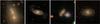 |
Fig. 2 Images of some galaxies in clusters. From left to right: the first ranked galaxy in the cluster A1750 with the colour index g − r = 0.72, (J131236.98-011151, BRG), a red spiral galaxy in the cluster A1066 (J10351.33+051130.8, g − r = 0.75, BRG), two galaxies in the cluster A1658 (J130116.68-032823.6 with g − r = 0.67, BRG, and J130116.09-032829.1 with g − r = 0.54), and a red spiral galaxy in the cluster A1663 (J130152.6-024012.3 with g − r = 0.75, BRG). |
The data for cluster galaxy populations are given in Table 3. Images of all galaxies in our clusters are shown on the web page http://www.aai.ee/~maret/SGWcl.html.
In the following analysis of individual rich clusters we present for each cluster the sky distribution of galaxies along with the density contours, the 3D vizualisation plot of galaxies (to generate these figures, we used the R package scatterplot3D by Ligges & Mächler 2003), the histograms of the peculiar velocities for galaxies of a different morphological type and for the BRGs, and the colour–magnitude diagrams. We have added the Gaussians for the components to the histograms of the peculiar velocities of all galaxies. For some clusters we include additional figures to show their substructure.
In the figures of the sky distribution of galaxies in clusters the 2D density contours are calculated with Mclust for clusters with more than one component, and with the Rpackage Kernsmooth for clusters with one component only.
4. Results
4.1. Clusters in the superclusters SCl 111 and SCl 91
4.1.1. The cluster A1066
The first rich cluster we study is the cluster A1066, which is located in the supercluster SCl 91. Figure 3 (left panel) shows that the 2D density contours of this cluster are quite smooth ellipsoids. According to Mclust, this cluster consists of one component, the mean uncertainty of the classification is 1.89 × 10⁻². However, the 3D distribution of galaxies in this cluster Fig. 3 (right panel) is complex – the shape resembles an hourglass, where some galaxies with negative peculiar velocities form a separate component.
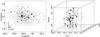 |
Fig. 3 2D and 3D view of the cluster A1066 (SCl 91). Open circles correspond to elliptical galaxies, crosses – to spiral galaxies, filled circles to BRGs, and a star to the first ranked galaxy in the cluster. |
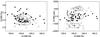 |
Fig. 4 Left panel shows RA vs. Dec, the right panel RA vs. peculiar velocities of galaxies (in km s-1) in the cluster A1066. Different symbols correspond to three different velocity components (see text), ellipses show the covariances of the components. |
Figure 4, a so-called classification plot produced by Mclust, shows three components in the distribution of the peculiar velocities of galaxies. The peculiar velocities with negative values correspond to the lower part of the “hourglass”. The left panel of this figure shows that the different components in velocity are not separated in the sky distribution, which is why Mclust determines one component only for this cluster as given in Table 2. We see three components in the distribution of the peculiar velocities of galaxies in this cluster, and the p-value of the Shapiro-Wilk test for this cluster is 0.074, the lowest among our sample (the lower the p-value, the higher is the difference to the Gaussian null hypothesis).
The histograms of the peculiar velocities for all galaxies and separately for the elliptical and spiral (and red spiral) galaxies and for the BRGs in A1066 are shown in Fig. 5. At the peculiar velocities vpec > 1000 km s-1 we see a small separate component of galaxies consisting mostly of spirals (including red spirals), although there are also some elliptical galaxies and one BRG among them; this system is also seen in Fig. 4. In the main component of this cluster the galaxies have peculiar velocities 1000 > vpec > − 500 km s-1, the first ranked galaxy of the cluster also belong here. At negative peculiar velocities (vpec ≤ − 500 km s-1) there is another extension (a lower part of the “hourglass” in Fig. 3, right panel) of galaxies, consisting again mostly of spirals, including red spirals and five BRGs. Eight of sixteen BRGs in this cluster have been classified as spirals (Table 3), five of them are located in this extension. The distribution of the peculiar velocities of elliptical galaxies shows a concentration towards the cluster centre, while the distribution of the peculiar velocities of spiral galaxies is smoother.
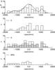 |
Fig. 5 Distribution of the peculiar velocities of galaxies in the cluster A1066. Top down: all galaxies, elliptical galaxies, spiral galaxies (the grey histogram shows the red spirals), and BRGs. P denotes the probability histogram, F the galaxy number counts. The small dash in the upper panel indicates the peculiar velocity of the first ranked galaxy. |
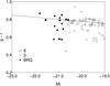 |
Fig. 6 Colour–magnitude diagram of galaxies in the cluster A1066. Empty circles denote elliptical galaxies, crosses spiral galaxies, filled circles BRGs. |
Galaxy populations in rich clusters.
In the colour–magnitude diagram for A1066 (Fig. 6) we show with separate symbols elliptical and spiral galaxies and BRGs. The slope and the rms scatter of the red sequence in the colour–magnitude diagram are presented in Table 3. 73% of the galaxies in this cluster are red, more than half of the red galaxies are spirals (or S0s). The colour–magnitude diagram shows that the scatter of colours of red spirals (both the red spiral BRGs and fainter red spirals) is larger than the scatter of colours of red elliptical galaxies (two faint blue galaxies in this cluster are classified as blue ellipticals), which suggests that red elliptical galaxies in this cluster form a more homogeneous population than red spiral galaxies. High negative and high positive peculiar velocities of some spiral galaxies and some BRGs in this cluster suggest that they dynamically form separate components of the cluster.
Summarizing, this cluster, classified by Mclust as a one-component cluster with a rather smooth sky distribution of galaxies has indeed a substructure, which suggests that this cluster has not yet completed its formation.
4.1.2. The cluster A1205
The sky distribution of galaxies in the cluster A1205 in the supercluster SCl 91 (Fig. 7, left panel) shows three different components. According to Mclust, this cluster even consists of five components, the mean uncertainty of the classification is 1.62 × 10⁻³. The reason for that is the distribution of the peculiar velocities of galaxies in each component that is shown in Fig. 9. This figure shows that the galaxies in a left component are divided into three according to their peculiar velocities; part of them have high positive peculiar velocities and others mostly negative peculiar velocities. There is also a small subcluster of galaxies with very low peculiar velocities.
In another big component the galaxies have mostly positive peculiar velocities, in the third one – negative peculiar velocities (Fig. 8). The shape of the 3D distribution of galaxies Fig. 7 (right panel) resembles an hourglass, this time seen at an angle.
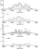 |
Fig. 8 Distribution of the peculiar velocities of galaxies in the cluster A1205. Top down: all galaxies, elliptical galaxies, spiral galaxies, and BRGs. The small dash in the upper panel indicates the peculiar velocity of the first ranked galaxy. |
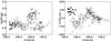 |
Fig. 9 Left panel shows RA vs. Dec, the right panel the RA vs. the peculiar velocities of galaxies (in km s-1) in the cluster A1205. Different symbols correspond to different velocity components. |
Even more interesting is the structure of this cluster if we plot the sky distribution with the density contours for red galaxies only (Fig. 10). This figure shows that one component in this cluster mostly consists of red galaxies (there are both elliptical and spiral galaxies among them, compare Fig. 7, left panel and Fig. 10).
The first ranked galaxy in this cluster is located almost at the centre of the sky distribution and has a very low peculiar velocity (the lowest among the clusters in our sample, see Table 2).
The histograms of the peculiar velocities of galaxies in A1205 in Fig. 8 show a large fraction of red spirals with negative peculiar velocites, which belong to the component with red galaxies. Some BRGs are also located there; in addition, we see several BRGs in other components, even at the edges of the cluster (Fig. 7). The peculiar velocities of galaxies from the three different components seen in the sky distribution partly overlap, so these components are not very clearly seen in the histograms.
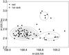 |
Fig. 10 Distribution of red galaxies (filled circles) in the cluster A1205. The star denotes the first ranked galaxy. |
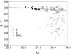 |
Fig. 11 Colour–magnitude diagram of galaxies in the cluster A1205. Empty circles denote elliptical galaxies, crosses spiral galaxies, filled circles BRGs. |
In the colour–magnitude diagram for the A1205 (Fig. 11) we see a bimodal distribution of galaxies, where the red and blue sequences are both clearly seen. This cluster has the largest fraction of blue galaxies in our sample (32%). The colour–magnitude diagram shows that the scatter of colours of red spirals is larger than the scatter of colours of red elliptical galaxies (the rms scatters are 0.033 and 0.027, correspondingly, for red spirals and for red ellipticals), although the difference is not as pronounced as in the cluster A1066. In this cluster there are four faint blue galaxies classified as blue ellipticals.
The presence of substructures in this cluster, which are populated by galaxies of different properties, suggests that the cluster A1205 consists of at least three merging components.
4.1.3. The cluster A1424
The next cluster under study, the cluster A1424, is located in the second rich supercluster in the SGW, SCl 111. The sky distribution of galaxies in this cluster (Fig. 12, left panel) shows two components also confirmed by Mclust. The mean uncertainty of the classification of galaxies in the cluster A1424 is 2.92 × 10⁻⁴.
The 3D distribution of galaxies (Fig. 12, right panel) shows that in one of these components galaxies have mostly positive peculiar velosities. Figure 13 shows that according to the sky distribution of galaxies in the cluster A1424, the components as delineated by elliptical and spiral galaxies are different – the two components are more clearly separated in the distribution of spiral galaxies.
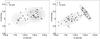 |
Fig. 13 Sky distribution of elliptical (left) and spiral (right) galaxies in the cluster A1424. The 2D density contours are calculated using the data about elliptical or spiral galaxies, respectively. Filled circles in the left panel denote elliptical galaxies, in the right panel spiral galaxies. The star denotes the first ranked galaxy. |
The distribution of the peculiar velocities of galaxies in the cluster A1424 (Fig. 14) has a minimum near the clusters centre, which is seen in the distribution of the peculiar velocities of both elliptical and spiral galaxies. The elliptical galaxies are more concentrated towards the centre of the cluster than the spiral galaxies, which is why the distribution of the peculiar velocities is smoother. In the same time, the distribution of the peculiar velocities of red spirals also shows two separate components. The BRGs are mostly located in the component with smaller right ascensions, several of which are spirals. The first ranked galaxy of this cluster is located almost in the centre of this component.
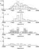 |
Fig. 14 Distribution of the peculiar velocities of galaxies in the cluster A1424. Top down: all galaxies, elliptical galaxies, spiral galaxies, and BRGs. The small dash in the upper panel indicates the peculiar velocity of the first ranked galaxy. |
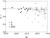 |
Fig. 15 Colour–magnitude diagram for galaxies in the cluster A1424. Empty circles denote elliptical galaxies, crosses spiral galaxies, filled circles BRGs. |
In this cluster 73% of all galaxies are red. In the colour–magnitude diagram (Fig. 15) the scatter of red spiral galaxies is about two times larger than the scatter of red elliptical galaxies (the rms scatters are 0.033 and 0.057, correspondingly, for red ellipticals and for red spirals). This is caused by galaxies in the outer parts of the cluster; it is possible that these galaxies have only recently joined the cluster.
4.1.4. The cluster A1516
The cluster A1516 is located in the high-density core of the supercluster SCl 111. The sky distribution of galaxies in this cluster shows very regular contours (Fig. 16, left panel). According to Mclust, this cluster has one component, the mean uncertainty of the classification of galaxies is 7.71 × 10⁻⁴.
The 3D distribution of galaxies shows that in the sky galaxies with negative peculiar velocities are mostly located in the central part of the cluster (Fig. 16, right panel, and Fig. 17), where they form an extension with the outer parts delineated mostly by spiral galaxies. This component is seen also in Fig. 18. According to the peculiar velocities, the elliptical galaxies in this component are concentrated towards the centre of the cluster. There is another peak in the distribution of the peculiar velocities of elliptical galaxies closer to the cluster centre; a signature of a past merger? The distribution of the peculiar velocities of spiral galaxies is less peaky. The distribution of the peculiar velocities of red spiral galaxies shows a concentration at the centre, at low peculiar velocites. There is also a small subcluster of galaxies with high positive peculiar velocities. The gradient of the peculiar velocities of galaxies in A1516 hints that this cluster may be rotating. With one exception, BRGs populate central parts of the cluster, and the first ranked galaxy of the cluster has a very low peculiar velocity, vpec = − 58 km s-1. The p-value of the Shapiro- Wilk test is 0.535, which confirms the Gaussian distribution of the peculiar velocities of galaxies in this cluster.
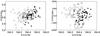 |
Fig. 17 Left panel shows RA vs. Dec, the right panel the RA vs. the peculiar velocities of galaxies (in km s-1) in the cluster A1516. Different symbols correspond to different velocity components. |
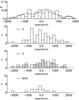 |
Fig. 18 Distribution of the peculiar velocities of galaxies in the cluster A1516. Top down: all galaxies, elliptical galaxies, spiral galaxies, and BRGs. The small dash in the upper panel indicates the peculiar velocity of the first ranked galaxy. |
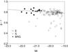 |
Fig. 19 Colour–magnitude diagram of galaxies in the cluster A1516. Empty circles denote elliptical galaxies, crosses spiral galaxies, filled circles BRGs. |
The colour–magnitude diagram in Fig. 19 shows that the scatter of colours of red ellipticals and red spirals is almost equal. The fraction of red galaxies in this cluster is very high (85%, Table 3), only 3 of 15 BRGs in this cluster are classified as spirals.
4.2. Clusters in the core of the supercluster SCl 126
4.2.1. The cluster A1650
The first cluster we study in the core of the supercluster SCl 126 is the cluster A1650, an X-ray cluster (Böhringer et al. 2004; Udomprasert 2004). This cluster is the second-poorest cluster in our sample with only 48 member galaxies in our catalogue. The sky distribution of galaxies in this cluster (Fig. 20, left panel) shows two concentrations. The 3D view and the velocity histograms of galaxies of different type (Fig. 20, right panel, and Fig. 21) show an almost separate component of galaxies with positive peculiar velocities, all but one galaxies in this component are elliptical. In the sky distribution this component is located almost in the centre of the cluster, thus Mclust, using the data about all the galaxies, finds that this cluster consists of one component, with the mean uncertainty of the classification 0.008. Red spiral galaxies and BRGs (with one exception) populate the main component of the cluster. Udomprasert (2004) describes this cluster as a compact X-ray source, possibly located at a cold spot in the CMB.
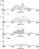 |
Fig. 21 Distribution of the peculiar velocities of galaxies in the cluster A1650. Top down: all galaxies, elliptical galaxies, spiral galaxies, and BRGs. The small dash in the upper panel indicates the peculiar velocity of the first ranked galaxy. |
However, the sky distribution of only elliptical or only spiral galaxies (Fig. 22) clearly shows two components in the distribution of elliptical and spiral galaxies, in both cases in a different manner. Thus we approximated the distribution of the peculiar velocities of galaxies with three Gaussians. These are better seen in the distribution of the peculiar velocities of elliptical galaxies. The distribution of the peculiar velocities of spiral galaxies is different. There is one spiral galaxy only in one component, which has the highest peculiar velocity in this component. Mclust confirms the components in the distribution of elliptical and spiral galaxies. The first ranked galaxy of this cluster is located at the edge of the elliptical galaxy component, but in the centre of one spiral galaxy component; the peculiar velocity of the first ranked galaxy vpec = − 189 km s-1.
The fraction of red galaxies in this cluster is very high, some spiral galaxies are also red. Owing to the small number of galaxies in this cluster the high fraction of red galaxies is only approximate. The first ranked galaxy in this cluster is also a red spiral galaxy, as seen in the colour–magnitude diagram (Fig. 23). In this diagram the rms scatter of colours of the red sequence is 0.036 for red ellipticals and 0.042 for red spirals.
Our analysis hints at a possibility that this cluster consists of two main components, some galaxies belong to a third subgroup with high positive peculiar velocities. Because of the small number of galaxies in this cluster our results about substructures should be taken as a suggestion only.
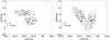 |
Fig. 22 Distribution of elliptical (left panel) and spiral (right panel) galaxies in the cluster A1650. Filled circles in left panel denote elliptical galaxies, in right panel they show spiral galaxies. The star is the first ranked galaxy. |
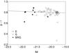 |
Fig. 23 Colour–magnitude diagram of galaxies in the cluster A1650. Empty circles denote elliptical galaxies, crosses spiral galaxies, filled circles BRGs. |
4.2.2. The cluster A1658
The next cluster we study in the core of the supercluster SCl 126 is the cluster A1658, the poorest cluster in our sample with only 29 member galaxies. The sky distribution of galaxies in this cluster (Fig. 24, left panel) shows three irregularly located concentrations. According to Mclust, using the data about all the galaxies, this cluster has one component, the mean uncertainty of the classification of galaxies is less than 10-5.
The distribution of the peculiar velocities of galaxies in A1658 is shown in Fig. 25. The distribution of the peculiar velocities of spiral galaxies shows two separate components, while the distribution of the peculiar velocities of elliptical galaxies has a central concentration, and two elliptical galaxies have high peculiar velocities. These distributions may be a signature of merging, which is more clearly seen in the distribution of the peculiar velocities of spiral galaxies. The p-value of the Shapiro-Wilk test is p = 0.937, the highest among our cluster sample, confirms the Gaussianity of the velocity distribution. The peculiar velocity of the first ranked galaxy in this cluster vpec = − 463 km s-1; this galaxy is located in the richest component of this cluster. There are BRGs in both components, and most of the red spiral galaxies belong to one component.
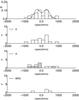 |
Fig. 25 Distribution of the peculiar velocities of galaxies in the cluster A1658. Top down: all galaxies, elliptical galaxies, spiral galaxies (grey – red spirals), and BRGs. The small dash in the upper panel indicates the peculiar velocity of the first ranked galaxy. |
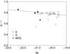 |
Fig. 26 Colour–magnitude diagram of galaxies in the cluster A1658. Empty circles denote elliptical galaxies, crosses spiral galaxies, filled circles BRGs. |
In the colour–magnitude diagram the scatter of colours of red galaxies in this cluster is very small, the fraction of red galaxies is high. Surprisingly, the scatter of colours of red spirals is even smaller than that of red ellipticals (with the rms values of 0.024 and 0.031, respectively). If the bimodal distribution of the peculiar velocities of galaxies in this cluster is an indication about a recent merger of two clusters into one, then the colour evolution of galaxies was probably already finished in these clusters before merging. Again, as we also mentioned with regard to the cluster A1650, the number of galaxies in this cluster is very small and our results concerning this cluster should be taken as suggestion.
4.2.3. The cluster A1663
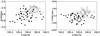 |
Fig. 28 Left panel shows RA vs. Dec, the right panel the RA vs. peculiar velocities of galaxies (in km s-1) in the cluster A1663. Different symbols correspond to different velocity components. |
Figure 27 shows that the distribution of galaxies in the cluster A1663 has a concentration where mostly galaxies with positive peculiar velocities are located. These galaxies form a separate component in the velocity distribution (Fig. 29). According to Mclust, this cluster has two components with the mean uncertainty of the classification 9.54 × 10⁻³.
The distribution of the peculiar velocities of all galaxies in A1663 in Fig. 29 shows three components. A concentration of the peculiar velocities near the cluster centre is mostly due to elliptical galaxies. The distribution of the peculiar velocities of spiral galaxies, especially that of red spirals, shows three subsystems, one of them corresponding to the component with high negative peculiar velocities. The p-value of the Shapiro-Wilk test is p = 0.37, so it does not confirm the non-Gaussianity of the velocity distribution. The BRGs in this cluster have peculiar velocities vpec < 500 km s-1, and in the sky distribution they are located at higher densities (according to the density contours in Fig. 27, where the first ranked galaxy is also located). The first ranked galaxy in this cluster has a high negative peculiar velocity (vpec = − 841 km s-1), suggesting that this cluster is not virialized yet. Burgett et al. (2004) suggest from the data from the 2dFGRS that the velocity gradient in this cluster is an indication that the cluster may be rotating.
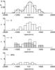 |
Fig. 29 Distribution of the peculiar velocities of galaxies in the cluster A1663. Top down: all galaxies, elliptical galaxies, spiral galaxies, and BRGs. The small dash in the upper panel indicates the peculiar velocity of the first ranked galaxy. |
 |
Fig. 30 Colour–magnitude diagram of galaxies in the cluster A1663. Empty circles denote elliptical galaxies, crosses spiral galaxies, filled circles BRGs. |
The fraction of red galaxies in the cluster A1663 is high, 83%, and 43% of red galaxies are spirals. In the colour–magnitude diagram the red and blue galaxies in this cluster are clearly separated. The scatter of colours of red galaxies in the cluster A1663 is larger than in the cluster A1658, with the rms value 0.037, and the scatter of colours of red ellipticals is larger than that of red spirals (with the rms values of 0.032 and 0.042, correspondingly).
4.2.4. The cluster A1750
The next cluster, which is the richest cluster in our sample with 117 member galaxies in our group catalogue, is the well-known binary merging Abell cluster A1750.
Mclust determined even five components in this cluster. In Fig. 31 (left panel) we mark them with numbers in an increasing order of the right ascencion. The mean uncertainty of the classification of galaxies in the cluster A1750 is 9.8 × 10⁻³.
 |
Fig. 32 Left panel shows RA vs. Dec, the right panel the RA vs. peculiar velocities of galaxies (in km s-1) in the cluster A1750. Different symbols correspond to different velocity components. |
The 3D distribution of galaxies in this cluster (Fig. 31, right panel) shows two almost separate components. In one of them most galaxies have negative peculiar velocities with a mean value vpec = − 600 km s-1. This component, marked as component 4 in the left panel of Fig. 31, is well seen in the classification diagram generated with Mclust, Fig. 32. The first ranked galaxy of the cluster A1750 is also located in this component and has the peculiar velocity vpec = − 724 km s-1. In Fig. 2 (left panel) we show an image of the first ranked galaxy in this cluster. This galaxy, a BRG, is embedded in a common red halo with its nearest companion galaxy which is the second in brightness in this cluster. These galaxies may form a merging system. The histograms of the peculiar velocites (Fig. 33) show that this component is better seen in the distribution of spiral galaxies than in the distribution of elliptical galaxies. Some BRGs are also located in component 4.
In Fig. 31 the 2D density contours show that the sky density of galaxies in the cluster A1750 is the highest in component 3. The mean peculiar velocity of galaxies in this component is vpec = − 72 km s-1. Several BRGs are located here.
In another component, component 5, galaxies have positive peculiar velocities, vpec = 612 km s-1. There are two BRGs in this component, and some elliptical and spiral galaxies.
In two components, 1 and 2, the mean peculiar velocity of galaxies is almost equal, vpec ≈ 220 km s-1, and the 2D density of galaxies decreases in these components as we move farther away from component 3 with a high 2D galaxy density. Figure 31 shows that also some BRGs are located in these components, in the outer parts of the cluster.
The distribution of the peculiar velocites of red spiral galaxies (Fig. 33) follows that of all spirals (of course, most spirals in this cluster are red).
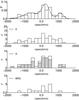 |
Fig. 33 Distribution of the peculiar velocities of galaxies in the cluster A1750. Top down: all galaxies, elliptical galaxies, spiral galaxies, and BRGs. |
The fraction of red galaxies in this cluster is very high (91%), and the rms scatter of colours of red elliptical and red spiral galaxies is almost equal, about 0.04. The colours of galaxies in different components are rather similar. In this respect the cluster A1750 differs from the cluster A1205, where one component consists mostly of red galaxies.
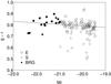 |
Fig. 34 Colour–magnitude diagram of galaxies in the cluster A1750. Empty circles denote elliptical galaxies, crosses spiral galaxies, filled circles BRGs. |
The structure of the cluster A1750 has been analysed in several other studies using optical and X-ray data (Donnelly et al. 2001; Belsole et al. 2004; Burgett et al. 2004; Hwang & Lee 2009). The comparison of substructures shows that our component 3 coincides with the component C by Hwang & Lee (2009). Belsole et al. (2004) finds an X-ray peak at this location and suggest that this component suffered a merger or interaction in the past 1–2 Gyr. Our component 4 is the same as the one determined by Hwang & Lee (2009) as component N, who suggest that the components 3 and 4 have started interacting. Component 4 coincides with another X-ray peak determined by Belsole et al. (2004). These are the same components denoted as Core and C in Burgett et al. (2004), and as the NW and SW components in Donnelly et al. (2001). Our components 1 and 2 correspond to a sparse component S by Hwang & Lee (2009), Belsole et al. (2004) shows an X-ray source in this direction. Hwang & Lee (2009) suggest that there has been past interaction between the components 1, 2, and 3. The component E in Hwang & Lee (2009) corresponds approximately to our component 5, and may have interacted in the past with both the components 3 and 4. Hwang & Lee did not find significant differences between the galaxy colours in different components, similar to our study.
Thus in the cluster A1750 our analysis reveals a similar substructure to that found in other studies.
4.3. The cluster A1773 in the outskirts of the supercluster SCl 126
The next cluster in our sample is the X-ray cluster A1773, the member of the supercluster SCl 126, which is located in the outskirts of the supercluster. The sky distribution of galaxies in this cluster is irregular, especially in the outer regions (Fig. 35, left panel). The 3D distribution of galaxies (Fig. 35, right panel) shows a component or tail of mostly elliptical galaxies and BRGs with negative peculiar velocities. The histograms of the peculiar velocities (Fig. 36) confirm that the brightest galaxies in this cluster have mostly negative peculiar velocities. They are located in one part of the sky distribution (see Fig. 35, left panel). The first ranked galaxy of the cluster is also located here, but has only a low peculiar velocity (vpec = − 76 km s-1). However, this subsystem of galaxies does not form a completely separate component; according Mclust, this cluster has one component with the mean uncertainty of the classification 0.041. The distribution of the peculiar velocities of spiral galaxies in this cluster is smoother than that of elliptical galaxies.
The fraction of red galaxies in the A1773 is 0.67 only. The scatter of colours of red ellipticals is smaller than that of red spirals (with the rms values of 0.032 and 0.047, correspondingly, see Table 3 and Fig. 37). If galaxies with negative peculiar velocities have only recently joined this cluster they have probably finished their colour evolution before joining the main cluster.
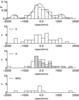 |
Fig. 36 Distribution of the peculiar velocities of galaxies in the cluster A1773. Top down: all galaxies, elliptical galaxies, spiral galaxies, and BRGs. The small dash in the upper panel indicates the peculiar velocity of the first ranked galaxy. |
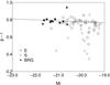 |
Fig. 37 Colour–magnitude diagram of galaxies in the cluster A1773. Empty circles denote elliptical galaxies, crosses spiral galaxies, filled circles BRGs. |
4.4. The cluster A1809 in the outskirts of the supercluster SCl 126
The last cluster in our sample is the cluster A1809 in the outskirts of the supercluster SCl 126. The sky distribution of galaxies in this cluster (Fig. 38, left panel) shows that this cluster consists of two components in the sky. Mclust also confirms that this cluster consists of two components with the mean uncertainty of classification 1.3 × 10⁻². In the main component of the cluster galaxies are concentrated in the center, and most BRGs of the cluster are also located here. The other component contains mostly loosely located spiral galaxies; there are also two elliptical galaxies and three BRGs, two of them located between this and the main component of the cluster. However, a word of caution is needed – in the poor component the number of galaxies is small, 17, the galaxies here are loosely distributed; it is possible that these galaxies cannot be considered as forming a reliable separate component. The 3D distribution of galaxies in the cluster A1809 (Fig. 38, right panel) and the distribution of the peculiar velocities of galaxies (Fig. 39) show that in the main component of the cluster the galaxies have a bimodal distribution of the peculiar velocities, which is best seen in the distribution for spiral galaxies. The velocity histograms show that some elliptical and spiral galaxies form a tail in the distribution of the peculiar velocities with high (vpec > 1000 km s-1) values of the peculiar velocities. The distribution of the peculiar velocities of red spiral galaxies follows those of all spirals. The velocity dispersion of the BRGs in this cluster is small, these galaxies are concentrated near the centre of the cluster. The distribution of the peculiar velocities of galaxies suggests that this cluster has formed by merging of two groups, and the third one (the poor component in the cluster A1809) is perhaps still infalling.
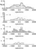 |
Fig. 39 Distribution of the peculiar velocities of galaxies in the cluster A1809. Top down: all galaxies, elliptical galaxies, spiral galaxies, and BRGs. The small dash in the upper panel indicates the peculiar velocity of the first ranked galaxy. |
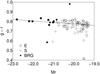 |
Fig. 40 Colour–magnitude diagram of galaxies in the cluster A1809. Empty circles denote elliptical galaxies, crosses spiral galaxies, filled circles BRGs. |
The fraction of red galaxies in the cluster A1809 is 0.84, similar to that in the clusters in the core of the supercluster. The scatter of colours of red ellipticals and red spirals (with the rms values of 0.029 and 0.032, correspondingly, see Table 3 and Fig. 40) is small. This suggests that the galaxies in the groups which formed the cluster A1809 possessed their final colours before merging.
The cluster A1809 has been studied for subclustering by Oegerle & Hill (1994, 2001), who found no substructure here. The reason for the difference between their results and ours may be the difference in the data used – in their study the cluster includes a smaller number of galaxies, and the smaller component is not well seen. As we mentioned above, it is also possible that the galaxies in the smaller component do not form a reliable separate component.
5. Discussion
5.1. Dynamical state of rich clusters
Our calculations with Mclust showed that among the ten clusters studied here five consist of more than one component, and the clusters A1205 and A1750 have the largest number of substructures. Even one-component clusters have several components in the distribution of the peculiar velocities of galaxies. In one cluster, A1205, one of the components is mostly populated by red galaxies, both ellipticals and spirals. In other clusters, the distribution of the peculiar velocities of galaxies shows that elliptical galaxies are more concentrated towards the cluster centre or towards the centres of subclusters, than spiral galaxies. This is possibly a signature of recent mergers that affects the morphology of galaxies in cluster. In the cluster A1773 we see the opposite – the velocity dispersion of spiral galaxies is lower than that of elliptical galaxies. This shows that the formation history of our clusters was different.
A word of caution is needed concerning the poorest clusters in our sample, the clusters A1650 and A1658: owing to the small number of galaxies in these clusters our results concerning them should be taken as a suggestion only. Even clusters with smaller numbers of galaxies have been studied for substructures (see, for example, Solanes et al. 1999; Boschin et al. 2008); however, Boschin et al. (2008) mention that clusters with about 30 member galaxies are too small for the analysis of the substructure (see also the discussion about the substructure statistics in small samples in Biviano et al. 2006).
Clusters with multiple components belong to all three superclusters of the SGW. Based on our earlier studies of the supercluster SCl 126, we assumed that clusters in the high-density core of this supercluster are dynamically more evolved than clusters in other superclusters of the SGW, and close to be virialized. Now we see that this is not so, clusters in the high-density cores of superclusters also have substructure and thus are not yet virialized.
Ragone-Figueroa & Plionis (2007) showed that in simulations group-size haloes located close to massive haloes have substructure. Plionis (2004) found that dynamically active clusters are more strongly clustered than the overall cluster population. Some studies of N-body models suggest that the fraction of haloes with substructure typically increases in high-density regions (Ragone-Figueroa & Plionis 2007, and references therein). In our study all clusters lie in superclusters, but we did not detect clear differences in the properties of clusters in the supercluster cores and in the outskirts or in the poor supercluster SCl 91.
We analysed the distribution of the peculiar velocities of galaxies in clusters. The number of galaxies in the clusters is not large, thus for the distribution of the peculiar velocities of galaxies we used the Shapiro-Wilk test to check the agreement with normality. In Table 2 we give the p-values of this test. These values show that the highest probability that the distribution of the peculiar velocities of galaxies in a cluster is not normal, is recorded for the cluster A1066, one-component cluster, in which the distribution of the peculiar velocities of galaxies shows three components, a possible indication of merging subgroups.
In Table 2 we give the values of kurtosis and skewness for the distributions of the peculiar velocities of galaxies in clusters (see also Solanes et al. 1999; Oegerle & Hill 2001; Boschin et al. 2006; Barrena et al. 2007; Hwang & Lee 2007). The positive values of kurtosis in Table 2 suggest that all distributions are peaked. The skewness shows that the distributions are asymmetrical, being skewed to the right or left, depending on the cluster. However, the p-values are higher than 0.05 showing that deviations from the normal distribution are statistically not very significant. The p-value for kurtosis for the cluster A1205 is low, for skewness it is high. These tests compare different aspects of the distributions, thus the results may not be similar. We also see that the results of the tests alone are not always good indicators for the possible substructure in the distributions. We saw that in the clusters with several components in the sky the distributions of the peculiar velocities of galaxies in different components sometimes (partly) coincide. Thus the low statistical significance for the deviations from normality is not surprising.
Another indicator of virialization of clusters is the peculiar velocity of the first ranked galaxy in cluster. In six clusters from our sample the peculiar velocities of the first ranked galaxies vpec > 180 km s-1. The relative peculiar velocities of the first ranked galaxies in our clusters, | vpec | / σv (Table 2) can be divided into three classes: four clusters have | vpec | / σv ≤ 0.20, two – | vpec | / σv = 0.41, and four clusters – | vpec | / σv ≥ 1.0. The low value of the relative peculiar velocity for the clusters A1205 and A1809 is misleading – the presence of multiple components in these clusters is a clear evidence of the nonvirialized state. Two other clusters with relative peculiar velocities less than 0.20σv are both one-component clusters. Both clusters with vpec/σv = 0.41, although they are one-component systems, have several components in the distribution of the peculiar velocities of galaxies. Four multicomponent clusters have the highest values of the relative peculiar velocities.
High peculiar velocities of the first ranked galaxies in clusters have been found in several recent studies (Oegerle & Hill 2001; Coziol et al. 2009). Some of the clusters in our sample and in the sample of rich clusters in Coziol et al. (2009) coincide; for common clusters our results agree well. The high peculiar velocities of the first ranked galaxies in clusters suggest that those clusters have not been yet virialized after a recent merger (Malumuth 1992), see also Oegerle & Hill (2001); )Coziol et al. (2009). Before merger, these galaxies were the first ranked galaxies of one group which merged to form a larger system. As evidence for that, we found that in several of our groups the first ranked galaxy is located near the centre of one component. In this respect the cluster A1205 is exceptional – in this cluster the first ranked galaxy lies between different components.
All rich clusters we studied correspond to Abell clusters. An identification of clusters is usually complicated because of the differences between the data in the catalogues. This is also the case here. We compared the data of our clusters with the data of Abell clusters from the catalogue by Andernach & Tago (2009, private communication). This comparison showed that often several our groups can be associated with one Abell cluster. Our cluster, which we identified with the Abell cluster A1066, is the richest cluster among the four groups which can be associated with this cluster; among the other groups one has 35 member galaxies, others are pairs of galaxies. Other clusters from the catalogue by Andernach & Tago (2009) can be associated with one rich cluster and one to four poor groups with up to five member galaxies. This also confirms the presence of substructure in rich clusters.
The cluster A1750 has been studied for substructure by other authors, too. We showed above that the components found in this cluster by us coincide well with those found in other studies. We found an especially good agreement between our results and those by Hwang & Lee (2009), who used used a Δ-test (Dressler & Shectman 1988) to determine the substructure in the cluster A1750. This shows that Mclust, probably applied here for the first time for the purpose to find substructure in galaxy clusters, gives results in agreement with other methods.
The good agreement with other studies also supports our choice of the parameters for the friend-of-friend algorithm for group definition and suggests that in our catalogue groups with substructure are real groups and not complexes of small groups artificially linked together by an unreasonable choice of linking parameters. This example supports our opinion that in the T10 the linking parameters were chosen reasonably.
An increasing number of studies have recently shown the presence of substructure in rich clusters (Solanes et al. 1999; Oegerle & Hill 2001; Burgett et al. 2004; Boschin et al. 2006; Barrena et al. 2007; Hwang & Lee 2007; Aguerri & Sanchez-Janssen 2010) and in poor clusters (Boschin et al. 2008); Vennik & Hopp (2009) found a substructure also in poor groups. Tovmassian & Plionis (2009) studied the properties of poor groups from the SDSS survey and showed that many groups of galaxies presently are not in a dynamical equilibrium but at various stages of virialization. Niemi et al. (2007) showed that a significant fraction of nearby groups of galaxies are not gravitationally-bound systems. This is important because the masses of observed groups are often estimated assuming that groups are bound.
The presence of substructure in rich clusters, signs of possible mergers, infall, or rotation suggests that the rich clusters in our sample are not yet virialized. The high frequency of these clusters tells us that mergers between groups and clusters are common – galaxy groups continue to grow. In high-density regions groups and clusters of galaxies form early and could be more evolved dynamically (Tempel et al. 2009), but here again the possibility of mergers is high, thus groups and clusters in high-density regions are still assembling.
5.2. Galaxy populations in rich clusters
The study of the galaxy content of the rich clusters showed in agreement with our earlier study (Einasto et al. 2008) that the fraction of red galaxies in clusters from the core of the supercluster SCl 126 is very high, Fred > 0.8. However, this is as large as the fraction of red galaxies in the cluster A1809 from the outskirts of this supercluster, as well as in the cluster A1516 from the supercluster SCl 111. We plot the fractions of red galaxies in clusters and the fractions of elliptical galaxies in Fig. 41. This figure shows that the fraction of elliptical galaxies in clusters is proportional to the fraction of red galaxies. At the same time the luminosities of clusters vary strongly, i.e. the fraction of red galaxies in clusters from our sample does not correlate well with the luminosity of clusters. In our earlier studies we found that the fraction of red galaxies is the highest in clusters in the cores of rich superclusters, both for low- and high-luminosity clusters (Einasto et al. 2007a).
We found that approximately 1/3 of red galaxies are spirals. Recent results of the Galaxy ZOO project (Masters et al. 2010) showed that indeed a large fraction of red galaxies are spirals, and almost all massive galaxies are red independently of their morphological type. The colour–magnitude diagrams show that in some clusters (A1066, A1205, A1424) the scatter of the colours of red spirals is larger than the scatter of the colours of red ellipticals, suggesting that red ellipticals form a more homogeneous population than red spirals.
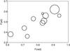 |
Fig. 41 Fractions of red galaxies and elliptical galaxies for our clusters. Symbol sizes are proportional to the luminosity of clusters. |
The number of BRGs in our clusters varies from four in A1658, which is the poorest cluster in our sample, to 17 in the richest cluster, A1750. Some BRGs are spirals. BRGs can be found both in the central areas and in the outskirts of clusters. The result that BRGs lie in clusters is consistent with the strong small- scale clustering of the LRGs (Zehavi et al. 2005; Eisenstein et al. 2005; Blake et al. 2008) that has been interpreted in the framework of the halo occupation model, where more massive haloes host a larger number of LRGs (van den Bosch et al. 2008; Zheng et al. 2009; Tinker et al. 2010; Watson et al. 2010).
The colours of galaxies in cluster environment may be affected by many factors. Colours may reach their observed values during a merging event when galaxies are affected by processes in the cluster environment (Berrier et al. 2009). For example, galaxies may be moved to the red sequence through the quenching of star formation in blue galaxies in the cluster environment (Bower et al. 1998; Ruhland et al. 2009; Bamford et al. 2009; Skelton et al. 2009). As evidence for that we found that in some of the clusters in our study the scatter of colours of galaxies is large, probably due to merging of components that affects the colours of galaxies.
At the same time Tinker et al. (2010) mention in the analysis of the distribution of distant red galaxies in the halo model framework that distant red galaxies must have formed their stars before they become satellites in haloes. This is possible if these galaxies were members of poorer groups before the groups merged into a richer one. We also find that in some clusters the range of red colours of galaxies is very small although these clusters consisted of several (probably merging) components. Probably in these cases the galaxies have finished their colour evolution in small groups before merging.
5.3. Merger analysis of dark matter haloes from simulation
The properties of the five most massive dark matter haloes.
5.3.1. Description of simulations
To illustrate the formation of present-day haloes via multiple mergers during their evolution in a cosmological simulations we present in this subsection merger histories of dark matter haloes in an N-body simulation.
We ran a ΛCDM simulation to study the merging history of dark matter haloes in a cosmological simulation. We used the GADGET-2 code (Springel et al. 2001; Springel 2005). In the simulation the dark matter haloes were identified with an algorithm called AHF (Amiga Halo Finder Knollmann & Knebe 2009), which is based on the adaptive grid structure of the simulation code in AMIGA (Adaptive Mesh Investigations of Galaxy Assembly). All haloes consist of the main halo – the most massive halo in the group, and subhaloes located within the virial radius sphere of the main halo.
For the simulation we adopted a cosmological ΛCDM model with (Ωm + ΩΛ + Ωb = 1) and h = 0.71, the dark matter density Ωdm = 0.198, the baryonic density Ωb = 0.042, the vacuum energy density ΩΛ = 0.76 and the rms mass density fluctuation parameter σ8 = 0.77. The simulation has 5123 dark matter particles, the volume of the simulation is 80 h-1 Mpc3. In this simulation the masses of the largest haloes are of the order of 1014 h-1 M⊙, the mass of an individual DM particle is 2.54 × 10⁸ h-1 M⊙. Our requirement for halo identification is that it has at least 100 particles, and therefore the minimum mass for haloes is 2.5 × 10¹⁰ h-1 M⊙. In the simulation, the main haloes with embedded subhaloes correspond to the observed groups and clusters of galaxies. Studies of substructure in observed groups and clusters of galaxies and in dark matter haloes in a similar manner provide an important probe for the formation of observed galaxy systems.
5.3.2. Halo mergers
The hierachical formation theory predicts that small haloes form first and large haloes are later assembled via mergers. To study the mergers between haloes during their formation, we calculated complete merger histories for the five richest (most massive) main haloes in the simulation. We focused on the late-time evolution, because it is more likely that the events occuring during this epoch may still be seen in the structure of the haloes.
In Table 4 we show the results of our analysis. We calculated the formation times for the main haloes, defined as the redshift when halo has half of its mass at the present epoch, and the mean value of the formation time for all the subhaloes with the standard deviation. We also show in Table 4 the total number of merger events for main haloes for z < 0.25 and the number of major mergers where the mass of the merging halo is at least 0.1 of the main halo mass.
 |
Fig. 42 Complete merger tree for a halo with ID = 1. Major merger events are indicated by circles with the size proportional to the mass of the merged halo. |
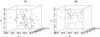 |
Fig. 44 Mclust results for haloes 1 and 3: 3D view of the components. |
To illustrate the complexity of halo histories, we show two examples of merger trees that we used for calculating the properties of mergers. In Fig. 42 we show the merger tree for the halo ID 1, which had three large recent merger events (at redshifts z = 0.0, 0.049, and 0.211). This halo has recently accreted its mass and its formation time is z = 0.271. This can be compared with the merger history for the halo ID 3, which has the same formation time and almost the same amount of recent mergers, but in this halo only one large merger event at redshift z = 0.1 is clearly visible. Thus the merger tree of halo ID 3 is quite different from that of halo ID 1 (Fig. 43). Interestingly, the mean value of the formation time for subhaloes in the halo ID 3 is lower than that of the halo ID 1. The number of components found by Mclust is 2 for the halo ID 1 and 1 for the halo ID 3 (Table 4 and Fig. 44). Qualitatively one can say that more active late-time merging is visible in the clustering properties of haloes at z = 0.
A similar analysis was carried out for the five most massive simulated haloes. Our results show that a late-time formation of the main haloes and a number of recent major mergers can cause a late-time subgrouping of haloes. A large scatter in the formation times for subhaloes hints towards late time merging (the standard deviation in the Col. 6). In general, we notice that the number of recent large merger events is the best indicator for additional clustering and that it is strongly correlated with the Mclust findings. To better understand the merging histories of dark matter haloes a study of a larger sample of haloes is needed.
6. Conclusions
We studied the properties of rich clusters in different superclusters in the SGW. Our conclusions are as follows:
-
1)
We showed with Mclust, a publicly available package in the R statistical environment, that the richest clusters in all superclusters of the SGW have substructure.
-
2)
There are components in the distribution of the peculiar velocities of galaxies in clusters both with multiple components and in one-component clusters – evidence of merging components.
-
3)
The peculiar velocities of the first ranked galaxies in clusters with multiple components are high.
-
4)
Most rich clusters in the supercluster SCl 126 and the richest cluster in the supercluster SCl 111 have a very high fraction of red galaxies (Fr > 80%). About 1/3 of red galaxies in clusters are spirals. In several clusters the scatter of colours of red elliptical galaxies in the colour–magnitude diagram is smaller than the scatter of colours of red spirals, suggesting that red elliptical galaxies form a more homogeneous population than red spiral galaxies. The presence of colour-related substructure in these clusters suggests that the colour evolution of galaxies in these clusters has already finished before merging into clusters.
-
5)
Our clusters host a large number of BRGs. Some BRGs are spirals. They can be found both in the central areas and in the outskirts of clusters.
-
6)
We calculated the complete merger trees for the richest dark matter haloes in an N-body simulation and showed that the late-time formation of the main haloes and the amount of recent major mergers can cause the late-time subgrouping of haloes.
Our results about the presence of substructure in rich clusters, signs of possible mergers, infall or rotation suggest that rich clusters in different superclusters of the Sloan Great Wall, including the cores of superclusters, are not yet virialized. The richest clusters in the SGW are still assembling.
As a next step in the study of substructures in groups and clusters, we plan to study a larger sample of groups and clusters, including poor groups of galaxies and low-density global environments.
h is the Hubble constant in units of 100 km s-1 Mpc-1.
Acknowledgments
We are pleased to thank the SDSS Team for the publicly available data releases. Funding for the Sloan Digital Sky Survey (SDSS) and SDSS-II has been provided by the Alfred P. Sloan Foundation, the Participating Institutions, the National Science Foundation, the US Department of Energy, the National Aeronautics and Space Administration, the Japanese Monbukagakusho, and the Max Planck Society, and the Higher Education Funding Council for England. The SDSS Web site is http://www.sdss.org/. The SDSS is managed by the Astrophysical Research Consortium (ARC) for the Participating Institutions. The Participating Institutions are the American Museum of Natural History, Astrophysical Institute Potsdam, University of Basel, University of Cambridge, Case Western Reserve University, The University of Chicago, Drexel University, Fermilab, the Institute for Advanced Study, the Japan Participation Group, The Johns Hopkins University, the Joint Institute for Nuclear Astrophysics, the Kavli Institute for Particle Astrophysics and Cosmology, the Korean Scientist Group, the Chinese Academy of Sciences (LAMOST), Los Alamos National Laboratory, the Max-Planck-Institute for Astronomy (MPIA), the Max-Planck-Institute for Astrophysics (MPA), New Mexico State University, Ohio State University, University of Pittsburgh, University of Portsmouth, Princeton University, the United States Naval Observatory, and the University of Washington. We thank our referee for detailed and constructive comments and suggestions which helped to improve the paper. The present study was supported by the Estonian Science Foundation grants Nos. 8005, 7146 and 7765, and by the Estonian Ministry for Education and Science research project SF0060067s08. This work has also been supported by the University of Valencia through a visiting professorship for Enn Saar and by the Spanish MEC project AYA2006-14056, “PAU” (CSD2007-00060), including FEDER contributions, and the Generalitat Valenciana project of excellence PROMETEO/2009/064. J.E. thanks Astrophysikalisches Institut Potsdam (using DFG-grant 436 EST 17/4/06), where part of this study was performed. P.H. was supported by the Societas Scientiarum Fennica, and Jenny and the Antti Wihuri foundation. P.N. was supported by the Academy of Finland. The cosmological simulations were run at the CSC – Scientific Computing center in Finland.
References
- Abazajian, K. N., Adelman-McCarthy, J. K., Agüeros, M. A., et al. 2009, ApJS, 182, 543 [NASA ADS] [CrossRef] [Google Scholar]
- Adelman-McCarthy, J. K., Agüeros, M. A., Allam, S. S., et al. 2008, ApJS, 175, 297 [NASA ADS] [CrossRef] [Google Scholar]
- Aguerri, J. A. L., & Sanchez-Janssen, R. 2010, A&A, 521, A28 [NASA ADS] [CrossRef] [EDP Sciences] [Google Scholar]
- Anscombe, F. J., & Glynn, W. J. 1983, Biometrika, 70, 227 [Google Scholar]
- Ashman, K. M., Bird, C. M., & Zepf, S. E. 1994, AJ, 108, 2348 [NASA ADS] [CrossRef] [Google Scholar]
- Bamford, S. P., Nichol, R. C., Baldry, I. K., et al. 2009, MNRAS, 393, 1324 [NASA ADS] [CrossRef] [Google Scholar]
- Bardelli, S., Zucca, E., Zamorani, G., Moscardini, L., & Scaramella, R. 2000, MNRAS, 312, 540 [NASA ADS] [CrossRef] [Google Scholar]
- Barrena, R., Boschin, W., Girardi, M., & Spolaor, M. 2007, A&A, 469, 861 [NASA ADS] [CrossRef] [EDP Sciences] [Google Scholar]
- Belsole, E., Pratt, G. W., Sauvageot, J., & Bourdin, H. 2004, A&A, 415, 821 [NASA ADS] [CrossRef] [EDP Sciences] [Google Scholar]
- Berlind, A. A., Frieman, J., Weinberg, D. H., et al. 2006, ApJS, 167, 1 [NASA ADS] [CrossRef] [Google Scholar]
- Berrier, J. C., Stewart, K. R., Bullock, J. S., et al. 2009, ApJ, 690, 1292 [NASA ADS] [CrossRef] [Google Scholar]
- Biviano, A., Murante, G., Borgani, S., et al. 2006, A&A, 456, 23 [NASA ADS] [CrossRef] [EDP Sciences] [Google Scholar]
- Blake, C., Collister, A., & Lahav, O. 2008, MNRAS, 385, 1257 [NASA ADS] [CrossRef] [Google Scholar]
- Blanton, M. R., & Roweis, S. 2007, AJ, 133, 734 [NASA ADS] [CrossRef] [Google Scholar]
- Blanton, M. R., Brinkmann, J., Csabai, I., et al. 2003a, AJ, 125, 2348 [NASA ADS] [CrossRef] [Google Scholar]
- Blanton, M. R., Hogg, D. W., Bahcall, N. A., et al. 2003b, ApJ, 592, 819 [NASA ADS] [CrossRef] [Google Scholar]
- Böhringer, H., Schuecker, P., Guzzo, L., et al. 2004, A&A, 425, 367 [NASA ADS] [CrossRef] [EDP Sciences] [Google Scholar]
- Boschin, W., Girardi, M., Spolaor, M., & Barrena, R. 2006, A&A, 449, 461 [NASA ADS] [CrossRef] [EDP Sciences] [Google Scholar]
- Boschin, W., Barrena, R., Girardi, M., & Spolaor, M. 2008, A&A, 487, 33 [NASA ADS] [CrossRef] [EDP Sciences] [Google Scholar]
- Bower, R. G., Kodama, T., & Terlevich, A. 1998, MNRAS, 299, 1193 [NASA ADS] [CrossRef] [Google Scholar]
- Burgett, W. S., Vick, M. M., Davis, D. S., et al. 2004, MNRAS, 352, 605 [NASA ADS] [CrossRef] [Google Scholar]
- Butcher, H., & Oemler, Jr., A. 1978, ApJ, 219, 18 [NASA ADS] [CrossRef] [Google Scholar]
- Coziol, R., Andernach, H., Caretta, C. A., Alamo-Martínez, K. A., & Tago, E. 2009, AJ, 137, 4795 [NASA ADS] [CrossRef] [Google Scholar]
- D’Agostino, R. B. 1970, Biometrika, 57, 679 [Google Scholar]
- Donnelly, R. H., Forman, W., Jones, C., et al. 2001, ApJ, 562, 254 [NASA ADS] [CrossRef] [Google Scholar]
- Dressler, A. 1980, ApJ, 236, 351 [NASA ADS] [CrossRef] [Google Scholar]
- Dressler, A., & Shectman, S. A. 1988, AJ, 95, 985 [NASA ADS] [CrossRef] [Google Scholar]
- Einasto, M., & Einasto, J. 1987, MNRAS, 226, 543 [NASA ADS] [CrossRef] [Google Scholar]
- Einasto, J., Saar, E., Kaasik, A., & Chernin, A. D. 1974, Nature, 252, 111 [NASA ADS] [CrossRef] [Google Scholar]
- Einasto, M., Einasto, J., Tago, E., Müller, V., & Andernach, H. 2001, AJ, 122, 2222 [CrossRef] [Google Scholar]
- Einasto, M., Einasto, J., Müller, V., Heinämäki, P., & Tucker, D. L. 2003a, A&A, 401, 851 [NASA ADS] [CrossRef] [EDP Sciences] [Google Scholar]
- Einasto, M., Jaaniste, J., Einasto, J., et al. 2003b, A&A, 405, 821 [NASA ADS] [CrossRef] [EDP Sciences] [Google Scholar]
- Einasto, M., Suhhonenko, I., Heinämäki, P., Einasto, J., & Saar, E. 2005, A&A, 436, 17 [NASA ADS] [CrossRef] [EDP Sciences] [Google Scholar]
- Einasto, M., Einasto, J., Tago, E., et al. 2007a, A&A, 464, 815 [NASA ADS] [CrossRef] [EDP Sciences] [Google Scholar]
- Einasto, M., Saar, E., Liivamägi, L. J., et al. 2007b, A&A, 476, 697 [NASA ADS] [CrossRef] [EDP Sciences] [Google Scholar]
- Einasto, M., Saar, E., Martínez, V. J., et al. 2008, ApJ, 685, 83 [NASA ADS] [CrossRef] [Google Scholar]
- Eisenstein, D. J., Annis, J., Gunn, J. E., et al. 2001, AJ, 122, 2267 [NASA ADS] [CrossRef] [Google Scholar]
- Eisenstein, D. J., Blanton, M., Zehavi, I., et al. 2005, ApJ, 619, 178 [NASA ADS] [CrossRef] [Google Scholar]
- Fraley, C., & Raftery, A. E. 2006, Technical Report, Dep. of Statistics, University of Washington, 504, 1 [NASA ADS] [Google Scholar]
- Gott, J. R. I., Jurić, M., Schlegel, D., et al. 2005, ApJ, 624, 463 [Google Scholar]
- Huchra, J. P., & Geller, M. J. 1982, ApJ, 257, 423 [NASA ADS] [CrossRef] [Google Scholar]
- Huertas-Company, M., Foex, G., Soucail, G., & Pelló, R. 2009, A&A, 505, 83 [NASA ADS] [CrossRef] [EDP Sciences] [Google Scholar]
- Hwang, H. S., & Lee, M. G. 2007, ApJ, 662, 236 [NASA ADS] [CrossRef] [Google Scholar]
- Hwang, H. S., & Lee, M. G. 2009, MNRAS, 397, 2111 [NASA ADS] [CrossRef] [Google Scholar]
- Ihaka, R., & Gentleman, R. 1996, J. Comput. Graph. Statis., 5, 299 [Google Scholar]
- Knebe, A., & Müller, V. 2000, A&A, 354, 761 [NASA ADS] [Google Scholar]
- Knollmann, S. R., & Knebe, A. 2009, ApJS, 182, 608 [NASA ADS] [CrossRef] [Google Scholar]
- Kofman, L. A., Einasto, J., & Linde, A. D. 1987, Nature, 326, 48 [NASA ADS] [CrossRef] [Google Scholar]
- Leisch, F. 2004, J. Stat. Soft., 11, 1 [Google Scholar]
- Ligges, U., & Mächler, M. 2003, J. Stat. Soft., 8, 1 [Google Scholar]
- Lintott, C. J., Schawinski, K., Slosar, A., et al. 2008, MNRAS, 389, 1179 [NASA ADS] [CrossRef] [Google Scholar]
- Loeb, A. 2009, JCAP, 03, 022 [Google Scholar]
- Malumuth, E. M. 1992, ApJ, 386, 420 [NASA ADS] [CrossRef] [Google Scholar]
- Martínez, V. J., & Saar, E. 2002, Statistics of the Galaxy Distribution (Boca Raton: Chapman & Hall/CRC) [Google Scholar]
- Martínez, V. J., Arnalte-Mur, P., Saar, E., et al. 2009, ApJ, 696, L93 [NASA ADS] [CrossRef] [Google Scholar]
- Masters, K. L., Mosleh, M., Romer, A. K., et al. 2010, MNRAS, 405, 783 [NASA ADS] [Google Scholar]
- Merritt, D. 1984, ApJ, 276, 26 [NASA ADS] [CrossRef] [Google Scholar]
- Mobasher, B., Dickinson, M., Ferguson, H. C., et al. 2005, ApJ, 635, 832 [NASA ADS] [CrossRef] [Google Scholar]
- Nichol, R. C., Sheth, R. K., Suto, Y., et al. 2006, MNRAS, 368, 1507 [NASA ADS] [CrossRef] [Google Scholar]
- Niemi, S., Nurmi, P., Heinämäki, P., & Valtonen, M. 2007, MNRAS, 382, 1864 [NASA ADS] [CrossRef] [Google Scholar]
- Oegerle, W. R., & Hill, J. M. 1994, AJ, 107, 857 [NASA ADS] [CrossRef] [Google Scholar]
- Oegerle, W. R., & Hill, J. M. 2001, AJ, 122, 2858 [NASA ADS] [CrossRef] [Google Scholar]
- Ostriker, J. P., & Tremaine, S. D. 1975, ApJ, 202, L113 [NASA ADS] [CrossRef] [Google Scholar]
- Ouchi, M., Shimasaku, K., Akiyama, M., et al. 2005, ApJ, 620, L1 [NASA ADS] [CrossRef] [Google Scholar]
- Park, C., & Choi, Y. 2009, ApJ, 691, 1828 [NASA ADS] [CrossRef] [Google Scholar]
- Park, C., & Hwang, H. S. 2009, ApJ, 699, 1595 [NASA ADS] [CrossRef] [Google Scholar]
- Plionis, M. 2004, in Outskirts of Galaxy Clusters: Intense Life in the Suburbs, ed. A. Diaferio, IAU Colloq., 195, 19 [NASA ADS] [Google Scholar]
- Ragone-Figueroa, C., & Plionis, M. 2007, MNRAS, 377, 1785 [NASA ADS] [CrossRef] [Google Scholar]
- Rose, J. A., Gaba, A. E., Christiansen, W. A., et al. 2002, AJ, 123, 1216 [NASA ADS] [CrossRef] [Google Scholar]
- Ruhland, C., Bell, E. F., Häußler, B., et al. 2009, ApJ, 695, 1058 [NASA ADS] [CrossRef] [Google Scholar]
- Shapiro, S. S., & Wilk, M. B. 1965, Biometrika, 52, 591 [Google Scholar]
- Skelton, R. E., Bell, E. F., & Somerville, R. S. 2009, ApJ, 699, L9 [NASA ADS] [CrossRef] [Google Scholar]
- Solanes, J. M., Salvador-Solé, E., & González-Casado, G. 1999, A&A, 343, 733 [NASA ADS] [Google Scholar]
- Springel, V. 2005, MNRAS, 364, 1105 [NASA ADS] [CrossRef] [Google Scholar]
- Springel, V., Yoshida, N., & White, S. D. M. 2001, New Astron., 6, 79 [Google Scholar]
- Tago, E., Saar, E., Tempel, E., et al. 2010, A&A, 514, A102 [NASA ADS] [CrossRef] [EDP Sciences] [Google Scholar]
- Tempel, E., Einasto, J., Einasto, M., Saar, E., & Tago, E. 2009, A&A, 495, 37 [NASA ADS] [CrossRef] [EDP Sciences] [Google Scholar]
- Tinker, J. L., Wechsler, R. H., & Zheng, Z. 2010, ApJ, 709, 67 [NASA ADS] [CrossRef] [Google Scholar]
- Tovmassian, H. M., & Plionis, M. 2009, ApJ, 696, 1441 [NASA ADS] [CrossRef] [Google Scholar]
- Turner, E. L., & Gott, III, J. R. 1976, ApJS, 32, 409 [NASA ADS] [CrossRef] [Google Scholar]
- Udomprasert, P. S. 2004, Ph.D. Thesis, California Institute of Technology, United States – California [Google Scholar]
- van den Bosch, F. C., Pasquali, A., Yang, X., et al. 2008, [arXiv:0805.0002] [Google Scholar]
- Venemans, B. P., Röttgering, H. J. A., Overzier, R. A., et al. 2004, A&A, 424, L17 [NASA ADS] [CrossRef] [EDP Sciences] [Google Scholar]
- Vennik, J., & Hopp, U. 2009, Astron. Nachr., 330, 998 [NASA ADS] [CrossRef] [Google Scholar]
- Vogeley, M. S., Hoyle, F., Rojas, R. R., & Goldberg, D. M. 2004, in Outskirts of Galaxy Clusters: Intense Life in the Suburbs, ed. A. Diaferio, IAU Colloq., 195, 5 [NASA ADS] [Google Scholar]
- Watson, D. F., Berlind, A. A., McBride, C. K., & Masjedi, M. 2010, ApJ, 709, 115 [NASA ADS] [CrossRef] [Google Scholar]
- Whitmore, B. C., & Gilmore, D. M. 1991, ApJ, 367, 64 [NASA ADS] [CrossRef] [Google Scholar]
- Zehavi, I., Eisenstein, D. J., Nichol, R. C., et al. 2005, ApJ, 621, 22 [NASA ADS] [CrossRef] [Google Scholar]
- Zeldovich, I. B., Einasto, J., & Shandarin, S. F. 1982, Nature, 300, 407 [NASA ADS] [CrossRef] [Google Scholar]
- Zheng, Z., Zehavi, I., Eisenstein, D. J., Weinberg, D. H., & Jing, Y. P. 2009, ApJ, 707, 554 [NASA ADS] [CrossRef] [Google Scholar]
All Tables
All Figures
|
Fig. 1 Distribution of groups with at least four member galaxies in the Sloan great wall region. Black circles correspond to the groups in the SGW, grey circles to the groups in the field. Circle sizes are proportional to a group’s size in the sky. Crosses show the location of rich clusters, and numbers are their ID numbers from Table 1. |
| In the text | |
|
Fig. 2 Images of some galaxies in clusters. From left to right: the first ranked galaxy in the cluster A1750 with the colour index g − r = 0.72, (J131236.98-011151, BRG), a red spiral galaxy in the cluster A1066 (J10351.33+051130.8, g − r = 0.75, BRG), two galaxies in the cluster A1658 (J130116.68-032823.6 with g − r = 0.67, BRG, and J130116.09-032829.1 with g − r = 0.54), and a red spiral galaxy in the cluster A1663 (J130152.6-024012.3 with g − r = 0.75, BRG). |
| In the text | |
|
Fig. 3 2D and 3D view of the cluster A1066 (SCl 91). Open circles correspond to elliptical galaxies, crosses – to spiral galaxies, filled circles to BRGs, and a star to the first ranked galaxy in the cluster. |
| In the text | |
|
Fig. 4 Left panel shows RA vs. Dec, the right panel RA vs. peculiar velocities of galaxies (in km s-1) in the cluster A1066. Different symbols correspond to three different velocity components (see text), ellipses show the covariances of the components. |
| In the text | |
|
Fig. 5 Distribution of the peculiar velocities of galaxies in the cluster A1066. Top down: all galaxies, elliptical galaxies, spiral galaxies (the grey histogram shows the red spirals), and BRGs. P denotes the probability histogram, F the galaxy number counts. The small dash in the upper panel indicates the peculiar velocity of the first ranked galaxy. |
| In the text | |
|
Fig. 6 Colour–magnitude diagram of galaxies in the cluster A1066. Empty circles denote elliptical galaxies, crosses spiral galaxies, filled circles BRGs. |
| In the text | |
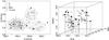 |
Fig. 7 2D and 3D views of the cluster A1205 (SCl 91). Symbols are the same as in Fig. 3. |
| In the text | |
|
Fig. 8 Distribution of the peculiar velocities of galaxies in the cluster A1205. Top down: all galaxies, elliptical galaxies, spiral galaxies, and BRGs. The small dash in the upper panel indicates the peculiar velocity of the first ranked galaxy. |
| In the text | |
|
Fig. 9 Left panel shows RA vs. Dec, the right panel the RA vs. the peculiar velocities of galaxies (in km s-1) in the cluster A1205. Different symbols correspond to different velocity components. |
| In the text | |
|
Fig. 10 Distribution of red galaxies (filled circles) in the cluster A1205. The star denotes the first ranked galaxy. |
| In the text | |
|
Fig. 11 Colour–magnitude diagram of galaxies in the cluster A1205. Empty circles denote elliptical galaxies, crosses spiral galaxies, filled circles BRGs. |
| In the text | |
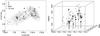 |
Fig. 12 2D and 3D views of the cluster A1424 (SCl 111). Symbols are the same as in Fig. 3. |
| In the text | |
|
Fig. 13 Sky distribution of elliptical (left) and spiral (right) galaxies in the cluster A1424. The 2D density contours are calculated using the data about elliptical or spiral galaxies, respectively. Filled circles in the left panel denote elliptical galaxies, in the right panel spiral galaxies. The star denotes the first ranked galaxy. |
| In the text | |
|
Fig. 14 Distribution of the peculiar velocities of galaxies in the cluster A1424. Top down: all galaxies, elliptical galaxies, spiral galaxies, and BRGs. The small dash in the upper panel indicates the peculiar velocity of the first ranked galaxy. |
| In the text | |
|
Fig. 15 Colour–magnitude diagram for galaxies in the cluster A1424. Empty circles denote elliptical galaxies, crosses spiral galaxies, filled circles BRGs. |
| In the text | |
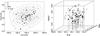 |
Fig. 16 2D and 3D views of the cluster A1516 (SCl 111). Symbols are the same as in Fig. 3. |
| In the text | |
|
Fig. 17 Left panel shows RA vs. Dec, the right panel the RA vs. the peculiar velocities of galaxies (in km s-1) in the cluster A1516. Different symbols correspond to different velocity components. |
| In the text | |
|
Fig. 18 Distribution of the peculiar velocities of galaxies in the cluster A1516. Top down: all galaxies, elliptical galaxies, spiral galaxies, and BRGs. The small dash in the upper panel indicates the peculiar velocity of the first ranked galaxy. |
| In the text | |
|
Fig. 19 Colour–magnitude diagram of galaxies in the cluster A1516. Empty circles denote elliptical galaxies, crosses spiral galaxies, filled circles BRGs. |
| In the text | |
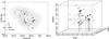 |
Fig. 20 2D and 3D views of the cluster A1650. Symbols are the same as in Fig. 3. |
| In the text | |
|
Fig. 21 Distribution of the peculiar velocities of galaxies in the cluster A1650. Top down: all galaxies, elliptical galaxies, spiral galaxies, and BRGs. The small dash in the upper panel indicates the peculiar velocity of the first ranked galaxy. |
| In the text | |
|
Fig. 22 Distribution of elliptical (left panel) and spiral (right panel) galaxies in the cluster A1650. Filled circles in left panel denote elliptical galaxies, in right panel they show spiral galaxies. The star is the first ranked galaxy. |
| In the text | |
|
Fig. 23 Colour–magnitude diagram of galaxies in the cluster A1650. Empty circles denote elliptical galaxies, crosses spiral galaxies, filled circles BRGs. |
| In the text | |
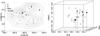 |
Fig. 24 2D and 3D view of the cluster A1658. Symbols are the same as in Fig. 3. |
| In the text | |
|
Fig. 25 Distribution of the peculiar velocities of galaxies in the cluster A1658. Top down: all galaxies, elliptical galaxies, spiral galaxies (grey – red spirals), and BRGs. The small dash in the upper panel indicates the peculiar velocity of the first ranked galaxy. |
| In the text | |
|
Fig. 26 Colour–magnitude diagram of galaxies in the cluster A1658. Empty circles denote elliptical galaxies, crosses spiral galaxies, filled circles BRGs. |
| In the text | |
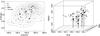 |
Fig. 27 2D and 3D views of the cluster A1663. Symbols are the same as in Fig. 3. |
| In the text | |
|
Fig. 28 Left panel shows RA vs. Dec, the right panel the RA vs. peculiar velocities of galaxies (in km s-1) in the cluster A1663. Different symbols correspond to different velocity components. |
| In the text | |
|
Fig. 29 Distribution of the peculiar velocities of galaxies in the cluster A1663. Top down: all galaxies, elliptical galaxies, spiral galaxies, and BRGs. The small dash in the upper panel indicates the peculiar velocity of the first ranked galaxy. |
| In the text | |
|
Fig. 30 Colour–magnitude diagram of galaxies in the cluster A1663. Empty circles denote elliptical galaxies, crosses spiral galaxies, filled circles BRGs. |
| In the text | |
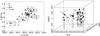 |
Fig. 31 2D and 3D views of the cluster A1750. Symbols are the same as in Fig. 3. |
| In the text | |
|
Fig. 32 Left panel shows RA vs. Dec, the right panel the RA vs. peculiar velocities of galaxies (in km s-1) in the cluster A1750. Different symbols correspond to different velocity components. |
| In the text | |
|
Fig. 33 Distribution of the peculiar velocities of galaxies in the cluster A1750. Top down: all galaxies, elliptical galaxies, spiral galaxies, and BRGs. |
| In the text | |
|
Fig. 34 Colour–magnitude diagram of galaxies in the cluster A1750. Empty circles denote elliptical galaxies, crosses spiral galaxies, filled circles BRGs. |
| In the text | |
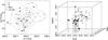 |
Fig. 35 2D and 3D views of the cluster A1773. Symbols are the same as in Fig. 3. |
| In the text | |
|
Fig. 36 Distribution of the peculiar velocities of galaxies in the cluster A1773. Top down: all galaxies, elliptical galaxies, spiral galaxies, and BRGs. The small dash in the upper panel indicates the peculiar velocity of the first ranked galaxy. |
| In the text | |
|
Fig. 37 Colour–magnitude diagram of galaxies in the cluster A1773. Empty circles denote elliptical galaxies, crosses spiral galaxies, filled circles BRGs. |
| In the text | |
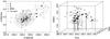 |
Fig. 38 2D and 3D views of the cluster A1809. Symbols are the same as in Fig. 3. |
| In the text | |
|
Fig. 39 Distribution of the peculiar velocities of galaxies in the cluster A1809. Top down: all galaxies, elliptical galaxies, spiral galaxies, and BRGs. The small dash in the upper panel indicates the peculiar velocity of the first ranked galaxy. |
| In the text | |
|
Fig. 40 Colour–magnitude diagram of galaxies in the cluster A1809. Empty circles denote elliptical galaxies, crosses spiral galaxies, filled circles BRGs. |
| In the text | |
|
Fig. 41 Fractions of red galaxies and elliptical galaxies for our clusters. Symbol sizes are proportional to the luminosity of clusters. |
| In the text | |
|
Fig. 42 Complete merger tree for a halo with ID = 1. Major merger events are indicated by circles with the size proportional to the mass of the merged halo. |
| In the text | |
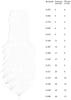 |
Fig. 43 Complete merger tree for a halo with ID = 3. Merger events as indicated in Fig. 42. |
| In the text | |
|
Fig. 44 Mclust results for haloes 1 and 3: 3D view of the components. |
| In the text | |
Current usage metrics show cumulative count of Article Views (full-text article views including HTML views, PDF and ePub downloads, according to the available data) and Abstracts Views on Vision4Press platform.
Data correspond to usage on the plateform after 2015. The current usage metrics is available 48-96 hours after online publication and is updated daily on week days.
Initial download of the metrics may take a while.