| Issue |
A&A
Volume 522, November 2010
|
|
|---|---|---|
| Article Number | A45 | |
| Number of page(s) | 7 | |
| Section | Interstellar and circumstellar matter | |
| DOI | https://doi.org/10.1051/0004-6361/201014875 | |
| Published online | 29 October 2010 | |
Photopolarimetric study of the star-forming clouds CB3, CB25, and CB39
1
Department of PhysicsAssam University,
Silchar 788011
Assam,
India
e-mail: This email address is being protected from spambots. You need JavaScript enabled to view it.
2
Istituto di Astrofisica Spaziale e Fisica Cosmica – Roma, Area di
Ricerca CNR Roma2 – Tor Vergata, V. Fosso del Cavaliere 100 I,
00133
Rome,
Italy
e-mail: This email address is being protected from spambots. You need JavaScript enabled to view it.
3
Department of Physics, GC College, Silchar 788005, Assam, India
e-mail: This email address is being protected from spambots. You need JavaScript enabled to view it.
4
IUCAA, Post Bag4, Ganeshkhinde, Pune
411007,
India
e-mail: This email address is being protected from spambots. You need JavaScript enabled to view it.
Received:
27
April
2010
Accepted:
28
June
2010
Abstract
Context. The small compact isolated dark clouds also known as “Bok globules” are believed to be ideal sites for low-mass star formation. Some of these clouds are undergoing gravitational collapse, and the ambient magnetic field plays a key role in collapse dynamics. The background star polarimetry is generally accepted as a good tool to map the magnetic field, which is responsible for the alignment of dichroic grains that produce polarization.
Aims. The background star polarization when studied together with extinction is expected to help us to understand various grain properties and the role of polarimetry as a tracer of magnetic field in these star-forming clouds. With this idea, polarization and colour excess E(B − V) values for a set of background stars have been studied together to understand various astrophysical process in some star-forming dark clouds.
Methods. Optical photometric observations of the three clouds CB3, CB25, and CB39 were carried out at the 2 m H.C. Telescope, India, to determine the colour excess E(B − V) of the background stars by following a technique adopted by Bernabei & Polacaro (2001, A&A, 371, 123). These three clouds were selected from a set of eight clouds previously observed by us in optical polarimetry (Sen et al. 2000, A&AS, 141, 175). Further independent spectroscopic measurements of a few selected sample stars were recently carried out during February and March 2010 from 1.52 m Cassini Telescope, Loinao, Italy, to confirm the correctness of estimated E(B − V) values obtained by this photometric technique.
Results. The colour excess E(B − V) values so obtained were compared with optical polarization values obtained for the same set of stars. It was found that the measured extinction values increase with the increase in percentage polarization for the cloud CB39 and to some extent for CB25. However, for cloud CB31 no such correlation was observed. It is normally expected that the grains causing extinction should also cause polarization of the light from background stars. Any possible deviation from this under different circumstances here has been discussed in the light of the ongoing physical processes in the star-forming clouds.
Key words: dust, extinction / ISM: clouds / stars: formation / techniques: photometric / polarization / techniques: spectroscopic
© ESO, 2010
1. Introduction
The small compact isolated dark clouds also known as “Bok gloubles” are believed to be sites for low mass star formation (Bok & Reilly 1947). For the clouds to be able to contract gravitationally to give birth to low-mass stars, they have to overcome the combined effect of thermal outward pressure, turbulence, and magnetic field. It is the magnetic field which plays a key role in collapse dynamics by mediating outflows, collimating jets, etc. The alignment of the magnetic field geometry in these clouds is generally mapped by background star polarimetry in the optical or NIR (near infra red).
Barnard (1927), Lynds (1962), and more recently Clemens & Bervainis (1988) have catalogued these small nearby molecular clouds.
When the light from the background stars passes through the clouds, extinction and reddening
are caused due to absorption and scattering by the dust grains present in the clouds. This
process also introduces polarization in the star light, if the grains are dichroic and
aligned. It is believed that the grains get aligned by an ambient magnetic field by a
mechanism originally suggested by Davis & Greenstein (1951) and subsequently modified by many authors. Recently, many photometric,
polarimetric, spectrometric, and radiometric studies have been reported on star-forming
clouds by various authors (Huard et al. 2000; Larson
et al. 2000; Sen et al. 2000; Wiebe & Watson 2001;
Khanzadyan et al. 2002; Launhardt & Sargent
2001; Matthews & Wilson 2002; Wolf-Chase et al. 2003; Draine 2003; Ghosh et al. 2005; Sen et al. 2005; Kandori et al. 2005; Massi et al.
2004, 2005;
Kirk et al. 2006; Gouliermis et al. 2006; Maheswar & Bhatt 2006; Naoi et al. 2006; Vaidya
et al. 2007; Ward-Thompson et al. 2000; Whittet 2007). It is generally expected that the
increasing extinction along a line of sight corresponds to increasing polarization.
Serkowski et al. (1975) found from their extensive
study of interstellar polarization at visual wavelengths, that while greater extinction
tended to go with greater polarization, a simple linear correlation did not exist. Jones
(1989) carried out a polarimetric study at
near-infrared wavelengths to investigate the behaviour of interstellar polarization as a
function of optical depth in front of a source for extinctions exceeding 100 mag
at V and found a good correlation between interstellar polarization
(p) and interstellar extinction at 2.2 μm for almost all
lines of sight. The observed trend in polarization with extinction was interpreted with a
model involving equal contributions from a uniform component and a random component to the
interstellar magnetic field. In most studies of the p vs.
AV relation, it is found that there is a
fuzzy upper bound to the amount of polarization possible for a particular extinction and
that observed points lie anywhere below this upper limit in the
p − AV line (Moneti et al.
1984; Whittet et al. 1994). Gerakines et al. (1995)
used polarimetric observations of background field stars to investigate alignment in the
Taurus Dark Cloud for extinctions in the magnitude range
0 < AK < 2.5
(equivalent to
0 < AV < 25)
and found a strong systematic trend in polarization efficiency with extinction, represented
by a power law  . The
result was discussed with a number of possible interpretations. Using near-IR polarimetry,
Goodman et al. (1992, 1995) found that there was almost no relation between the background star
polarization and extinction in the dark clouds. Arce et al. (1998) studied the relation between polarization (p) and
extinction (AV) in the Taurus cloud complex.
They found two trends in their
p − AV study: (1) stars
that are background to the warm interstellar medium show an increase in p
with AV; and (2) the polarization of stars that
are background to cold dark clouds does not increase with extinction. They offered a set of
guidelines to find where the polarization maps can be taken as faithful representations of
the magnetic field projected onto the plane of the sky and where they can not be. Fosalba
et al. (2002) made a statistical analysis of the
largest compilation available on the Galactic starlight polarization data and found a nearly
linear growth of mean polarization degree with extinction. The amplitude of this correlation
shows that interstellar grains are not fully aligned with the Galactic magnetic field, which
can be interpreted as the effect of a large random component of the field. Jones (2003) studied polarimetry at 1.65 μm of
stars shining through the filamentary dark cloud GF 9 and found the dust grains within GF 9-
core were aligned and produced polarization in extinction. Sen et al. (2005) modelled the dark cloud as a simple dichroic polarizing sphere,
which explains why polarization need not always increase with total extinction
AV as one moves towards the center of the
cloud. Their analysis shows that the observed polarization depends largely on the
orientation of the magnetic field (within the cloud) with respect to the direction of
interstellar magnetic field. The cause of the lack of polarizing power for dust in some cold
dark clouds is still debated.
. The
result was discussed with a number of possible interpretations. Using near-IR polarimetry,
Goodman et al. (1992, 1995) found that there was almost no relation between the background star
polarization and extinction in the dark clouds. Arce et al. (1998) studied the relation between polarization (p) and
extinction (AV) in the Taurus cloud complex.
They found two trends in their
p − AV study: (1) stars
that are background to the warm interstellar medium show an increase in p
with AV; and (2) the polarization of stars that
are background to cold dark clouds does not increase with extinction. They offered a set of
guidelines to find where the polarization maps can be taken as faithful representations of
the magnetic field projected onto the plane of the sky and where they can not be. Fosalba
et al. (2002) made a statistical analysis of the
largest compilation available on the Galactic starlight polarization data and found a nearly
linear growth of mean polarization degree with extinction. The amplitude of this correlation
shows that interstellar grains are not fully aligned with the Galactic magnetic field, which
can be interpreted as the effect of a large random component of the field. Jones (2003) studied polarimetry at 1.65 μm of
stars shining through the filamentary dark cloud GF 9 and found the dust grains within GF 9-
core were aligned and produced polarization in extinction. Sen et al. (2005) modelled the dark cloud as a simple dichroic polarizing sphere,
which explains why polarization need not always increase with total extinction
AV as one moves towards the center of the
cloud. Their analysis shows that the observed polarization depends largely on the
orientation of the magnetic field (within the cloud) with respect to the direction of
interstellar magnetic field. The cause of the lack of polarizing power for dust in some cold
dark clouds is still debated.
The present study aims at finding any possible relation between the observed polarization and extinction of the star, background of these clouds. For that purpose, three clouds CB3, CB25, and CB39 have been observed photometrically. The collected photometric data were reduced and analysed and then compared with the polarimetric data earlier reported by Sen et al. (2000). For some selected sample stars in some clouds independent spectroscopic measurements were also made. The results obtained from these three sets of independent polarimetric, photometric, and spectroscopic measurements are discussed with possible interpretations.
Calibrated B, V, R magnitudes, the computed E(B − V) and p for stars in CB3.
Calibrated B, V, R magnitudes, the computed E(B − V) and p for stars in CB25.
Calibrated B, V, R magnitudes, the computed E(B − V) and p for stars in CB39.
Computed and measured E(B − V) values for sample stars in CB25 and CB39.
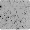 |
Fig. 1 CCD image of the cloud CB3. Star numbers refer to Table 1 (Field centre: RA = 00:28:45.8, Dec = 56:42:08) (J2000). All star numbers have been placed just below the corresponding star in the image. |
2. Observation
Polarimetric observations of a set of eight Bok globules CB3, CB25, CB39, CB52, CB54, CB62, and CB246 were made previously by Sen et al. (2000). From the given list of eight clouds, three clouds CB3, CB25, and CB39 have been observed photometrically for the present study. These three clouds were selected at random from the set of eight clouds, based on their availability at the time of observation. Photometric observations, with the Bessell filters B [486.1(10)], V [500.7(10)] and R [656.3(10)], of the three clouds were carried out in two nights of 2004 January 24 and 25. The observations were carried out at the cassegrain focus (f/9 beam) of 2 m Himalayan Chandra Telescope (lat.= 32°46′46′′ N; long. = 78057′51′′ E ; alt. = 4500 m) of Indian Astronomical Observatory, Hanle (remotely operated from CREST, Bangalore, India via a dedicated satellite link). A 2048 × 4096 EEV CCD detector was used with 15 micron pixel size, which has 0.296 arcsec/pixel scale and 10.1 × 10.1 arcmin field of view. The seeing condition was around 1.5′′ at the time of observation.
Figure 1 shows the CCD image of the cloud CB3 with the field stars numbered, as in Table 1. The images of all the clouds with their background stars included in the present work are available from our previous work (Sen et al. 2000).
Further spectroscopic measurements of stars in CB25 and in CB39 were made from the 1.52 m INAF-OAB Cassini Telescope, at Loiano, Italy, during the nights of 2010 February 13 and March 27.
3. Data reduction and analysis
The basic photometric reductions (bias-subtraction, flat-fielding) of the CCD images of CB3, CB25, and CB39 in the B, V, R bands were carried out within the standard IRAF routines. The observed magnitudes of the stars in the B, V, R bands were estimated using aperture photometry within the IRAF task APPHOT, along with the photometric standard stars from the fields GSC 00012-00261 and GSC 04737-00114. These observed magnitudes were then corrected for atmospheric extinction at different airmass(X) values, using the extinction coefficients available from Parihar et al. (2003). After this photometric procedure, the final calibrated observed magnitudes of stars in the three clouds CB3, CB25, and CB39 are reproduced in Tables 1−3 respectively.
In Fig. 2 a colour − colour diagram with (B0 − V0) vs. (V0 − R0) for the stars in CB3 was drawn from the calibrated observed magnitudes (henceforth denoted as B0, V0 and R0). A similar procedure has been followed in Fig. 3 for CB25 and in Fig. 4 for CB39.
3.1. Calculation of colour excess
Determination of colour excess requires knowledge of the observed magnitudes and unreddened/dereddened intrinsic magnitudes of the stars, the later to be possibly determined through spectroscopy.
In order to determine the colour excess of all stars considered in the present work, the procedure adopted by Bernabei & Polcaro (2001), combined with the Cardelli et al. (1989)’s RV-dependent empirical relationships A(λ) / A(V), was followed. This is an iterative procedure, based on the fact that the intrinsic colours of main sequence stars are related to each other. We thus used an empirical relationship (details are in Bernabei & Polcaro 2001) to evaluate a “computed” (B − V) colour for each star corresponding to the observed (V − R). In this way, a first order approximated E(B − V) was obtained for each star. Dereddened B, V, and R magnitude were then computed from this colour excess, using the relationships given by Cardelli et al. (1989). This procedure was then repeated up to the convergence to zero of the residual colour excess, which was reached only after a certain number of iterations for all stars of the field. The total colour excess E(B − V) value was then computed. This technique is valid for main sequence stars only; on the other hand, the procedure has been checked on other occasions by comparing the derived colour excess with the ones obtained by other methods and was found to be working properly (Bernabei & Polcaro 2001).
The value of RV depends on the environment along the line of sight. A direction through low-density interstellar medium usually has a low value of RV ( ≃ 3.1). Lines of sight penetrating into a dense cloud usually show 4 ≤ RV ≤ 6 (Cardelli et al. 1989). As it is not possible to estimate RV quantitatively from the environment of a line of sight, for the present calculations RV has been taken as 4. However, E(B − V) values have also been calculated, taking RV = 3.1 and the results are reproduced in Tables 1 − 3 for clouds CB3, CB25, and CB39 respectively. These tables contain star numbers, calibrated magnitudes (cal. mag.) in B, V, R filters, the computed E(B − V) for RV = 3.1 and RV = 4 with respective error values (shown within the first brackets in Cols. 5 and 6) and the corresponding polarization values (p) of the field stars. As can be seen, the value of RV does not have a large effect on the computed E(B − V). The Bernabei & Polcaro (2001) procedure of determination of E(B − V) only involves photometric data.
In order to verify the correctness of the above procedure, we also made spectroscopic measurements of few sample stars in the CB25 and CB39 clouds from the 1.52 m La Cassini Telescope, Loiano, Italy. Two series of spectra of stars no. 9 and 15 in CB25 and star no. 8 in CB39 in the ranges 3300 − 5350 Å (Δλ = 1.7 Å/pixel) and 4200 − 6600 Å (Δλ = 1.0 Å/pixel) were obtained on February 13, 2010. These spectra were used for spectral classification and for the evaluation of the values of E(B − V) from a NaI D1 line equivalent width, following the calibration of Munari & Zwitter (1997), and from the central depth of the diffuse band at 4430 Å (Wu et al. 1981). Furthermore, low-resolution spectra in the range 3800 − 7000 Å (Δλ = 3.97 Å/pixel) of stars no. 9 and star no. 15 in CB25 were taken on March 27, 2010 and were flux calibrated by comparison with the spectrophotometric standard Feige 56 (A0V). The reddening was then evaluate by a comparison with the corresponding Kurucz (1979) model. The results are shown in Table 4, where computed (through photometry) and measured (through spectroscopy) E(B − V) values are compared. As can be seen for E(B − V), the measured (spectroscopic) values agree well with the computed (photometric) values.
Because spectroscopic observations demand more telescope time, we adopted the above indirect photometric technique from Bernabei & Polcaro (2001). And through the measurement of a few sample stars in two clouds, we verified the correctness of this photometric technique to determine E(B − V).
3.2. Error analysis
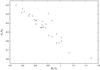 |
Fig. 2 (B0 − V0) vs. (V0 − R0) plot of the field stars(CB3) (colour − colour plot). |
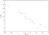 |
Fig. 3 (B0 − V0) vs. (V0 − R0) plot of the field stars (CB25). |
The sources of “noise” in the present photometric analysis are in the readout and photon
noise in the signal from the object. The signal-to-noise ratio of the object is estimated
from the data values in the following way using the standard relation
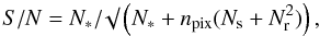 (1)where,
N∗ is the total(sky subtracted) source count,
npix is the number of pixels contained within the software
aperture, Ns, is the background sky count per pixel and
Nr is the read noise in electrons per pixel (Howell 1989). The N∗,
Ns are derived in net number of electrons (counts multiplied
by gain). In the present case, Gain =1.22 e − /ADU, Read noise =4.8
e − .
(1)where,
N∗ is the total(sky subtracted) source count,
npix is the number of pixels contained within the software
aperture, Ns, is the background sky count per pixel and
Nr is the read noise in electrons per pixel (Howell 1989). The N∗,
Ns are derived in net number of electrons (counts multiplied
by gain). In the present case, Gain =1.22 e − /ADU, Read noise =4.8
e − .
The estimated error of the magnitude in the aperture is approximately given by merr = 1.0857 × ( △ N∗/N∗), where △ N∗ is the measurement error (in electrons) of the estimated number of electrons from the star within the aperture (Davis 1987; Mighell 1999).
The errors in extinction coefficients (k) in the B, V, R bands are △ k(B) = 0.029, △ k(V) = 0.032, △ k(R) = 0.037 (Parihar et al. 2003) and the range of air mass(X) was [1.042 − 1.487].
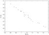 |
Fig. 4 (B0 − V0) vs. (V0 − R0) plot of the field stars (CB39). |
4. Results and discussions
Because the computed E(B − V) extinction values are not high, one may think that the observed extinction is purely due to interstellar medium and the foreground cloud makes no contribution to it. However, the optical polarization values observed for the same set of stars as reported here (for example CB3) have been found to be related to the sub-mm polarization values (Ward-Thompson et al. 2009). These two sets of polarization vectors were found to be tracing the same magnetic field prevalent in the cloud. Based on these findings, it can be claimed here that the optical polarization values which are included here for the analysis, are tracing the physical conditions within the clouds. Plots of p (from Sen et al. 2000) vs. E(B − V)) for all the three clouds with RV = 3.1 and 4.0 are reproduced in Figs. 5 and 6, with first p as dependent and then as independent variable. The error-weighted (for both variables) least-squares linear fit was made (York 1966) and the coefficients of correlation r were calculated (cf. Table 5).
For the cloud CB3 (Table 1), the mean value of the computed E(B − V) is found to be =0.27 and 0.28 for RV = 3.1 and 4 respectively. It is obvious from the colour − colour diagram (Fig. 2) that all stars fit a single main sequence. It is found (cf. Table 5) that the correlation coefficients for the cloud CB3 are 0.18 and 0.19. Thus it appears there is very low dependence of polarization on extinction for the cloud CB3.
For the cloud CB25 (cf. Table 2), the mean value of the computed E(B − V) is found to be =0.41 and 0.43 for RV = 3.1 and 4 respectively. It is seen that apart from stars no. 6 and 8, all other stars fall in the main sequence (Fig. 3). Accordingly, it is logical to assume that these two stars are non-main sequence stars, and we thus excluded them from the plot of colour excess vs polarization values (Figs. 5 and 6). With the other nineteen stars, the average values of E(B − V) are 0.44 and 0.46, for the above two RV values. The correlation coefficients for the cloud CB25 are 0.24 and 0.24 (Table 5). From the plots of p vs. E(B − V) for nineteen stars (Figs. 5 and 6), it is observed that the polarization may be linearly related to extinction, but the dependence is not so strong.
The mean values of the computed E(B − V) (Table 3) for the cloud CB39 are 0.67 and 0.72 for RV = 3.1 and 4 respectively. It is evident from the colour − colour diagram (Fig. 4) that all stars belong to the main sequence. It is clear from the plot (Figs. 5 and 6) and from the correlation coefficients (Table 5) that the polarization increases linearly with extinction. Here the values of the coefficient of correlation are 0.75 and 0.74 (for two values of RV), which are relatively higher.
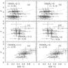 |
Fig. 5 Polarization p vs extinction E(B − V) for the clouds CB3, CB25, and CB39 for RV = 3.1 and 4.0 are shown. The dashed line in the figure represents the error-weighted least-square linear fit with E(B − V) as independent variable, to the data points in Tables 1–3 considering the errors in both variables. The “error bars” shown in the figures represent errors in p (taken from Sen et al. 2000) and errors in E(B − V) as derived in the present work. |
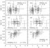 |
Fig. 6 Extinction E(B − V) vs. polarization p for the clouds CB3, CB25, and CB39 for RV = 3.1 and 4.0 are shown. The dashed line in the figure represents the error-weighted least-square linear fit with p as independent variable, to the data points in Tables 1–3, considering the errors in both variables. The “error bars” shown in the figures represent errors in p (taken from Sen et al. 2000) and errors in E(B − V) as derived in the present work. |
In the above we have computed E(B − V) with RV = 4 and also with RV = 3.1, because the latter is meaningful for IS medium and can serve as a reference. However, it is important to note here that the presence of (or lack of) a correlation between E(B − V) and p cannot depend on the value of RV. But if RV changes across the cloud, then this could mask a correlation. But the differences between the two computed values for E(B − V) in the Tables 1 − 3 are much smaller than the photometric errors we are dealing with here. We should also note that at very low E(B − V), any intrinsic polarization will dominate the interstellar component. Many of the stars towards CB3 and CB39 appear to have polarizations well above the maximum expected for the low extinction. Also CB39, which shows a correlation, has comparatively more stars at higher extinctions than other two.
Correlation coefficient (r), turbulence and T2 values for the clouds CB3, CB25 and CB39.
Higher grain alignment should result in a higher value of polarization. Assuming the Davis & Greenstein (1951) like alignment, Sen et al. (2005) had earlier quantified the degree of alignment by the parameter ~ T2 = Td/(Td + Tg), where Td and Tg are dust and gas temperatures. We can see from Table 5, that the correlation r also increases with T2. This implies that better grain alignment can also result in higher correlation between p and E(B − V). However, with just three data points it is difficult to draw a general conclusion. A higher number of these clouds should be investigated along these lines in future. Because, classical Davis & Greenstein model has long since been shown to be inadequate, in any future studies other grain alignment models (Lazarian et al. 1997) should be considered.
A lack of correlation between p and E(B − V) is also possible if there are two or more grain populations, one causing polarization and other causing extinction. From Figs. 5 and 6 for cloud CB39, one can see that when E(B − V) becomes zero, p correspondingly also becomes almost zero. This is consistent with a simple situation, where we have a single grain population causing both linear polarization and extinction in the line of sight.Thus when there is no extinction, we should have no polarization. Also the extinction and polarization will be expected to follow a good correlation. However, this is not seen for the other two clouds, indicating a more complex situation, which may include the possibility of multiple grain populations.
Conclusions
Based on the above analysis, one may conclude that
-
1.
The three clouds under observation show different degrees ofcorrelation between polarization and extinction. The correlationdoes not appear to be related to the turbulence or other parameterswithin the clouds.
-
2.
The correlation seems to be dependent on the degree of grain alignment (expressed as a function of dust and gas temperatures) as estimated using a Davis Greenstein type mechanism. However, for any future work to study this possibility, recent alignment models should be included.
-
3.
For any future studies, one should also determine E(B − V) more accurately with spectroscopy and perform polarimetry at much higher extinction in the infrared, with larger data sets.
Acknowledgments
We are grateful to the Inter University Centre for Astronomy and Astrophysics (IUCAA), Pune, India, for making grants available under its guest observing programme, to carry out this work. We thank the Indian Institute of Astrophysics, Bangalore, India, for the allotment of telescope time in the 2 m Himalayan Chandra Telescope. We are also grateful to the Loiano Observatory, Italy, for allotment of service observing time in the INAF-OAB 1.52 m Cassini Telescope (Loiano, Italy). We are particularly grateful to Roberto Gualandi, who performed in our behalf the observations and the related data reduction. Finally, we acknowledge the anonymous referee for valuable comments.
References
- Arce, H. G., Goodman, A. A., Bastein, P., Manset, N., & Summer, M. 1998, ApJ, 499, L93 [NASA ADS] [CrossRef] [Google Scholar]
- Barnard, E. E. 1927, in Atlas of Selected Regions of the Milky way, ed. E. Frost, & M. Calvert (Washington: Carnegie Institute), 247 [Google Scholar]
- Bernabei, S., & Polcaro, V. F. 2001, A&A, 371, 123 [NASA ADS] [CrossRef] [EDP Sciences] [Google Scholar]
- Bok, B. J., & Reilly, E. F. 1947, ApJ, 105, 255 [NASA ADS] [CrossRef] [Google Scholar]
- Cardelli, J. A., Clayton, G. C., & Mathis, J. S. 1989, ApJ, 345, 245 [NASA ADS] [CrossRef] [Google Scholar]
- Clemens, D. P., & Barvainis, R. 1988, ApJS, 68, 257 [NASA ADS] [CrossRef] [Google Scholar]
- Clemens, D. P., Yun, J. L., & Heyer, M. H. 1991, ApJ, 75, 877 [Google Scholar]
- Creese, M. P., & Jones, T. J. 1995, AJ, 110, 268 [NASA ADS] [CrossRef] [Google Scholar]
- Davis, Jr. L., & Greenstein, J. L. 1951, ApJ, 114, 206 [Google Scholar]
- Davis, L. 1987, Specifications for the Aperture Photometry Package, National Optical Astronomy Observatories [Google Scholar]
- Draine, B. T. 2003, ApJ, 598, 1017 [NASA ADS] [CrossRef] [Google Scholar]
- Fosalba, P., Lazarian, A., Prunet, S., & Tauber, J. A. 2002, ApJ, 564, 762 [NASA ADS] [CrossRef] [Google Scholar]
- Gerakines, P. A., Whittet, D. C. B., & Lazarian, A. 1995, ApJ, 455, L171 [NASA ADS] [CrossRef] [Google Scholar]
- Ghosh, S. K. 2005, BASI, 33, 133 [NASA ADS] [Google Scholar]
- Goodman, A. A., Jones, T. J., Lada, E. A., & Myers, P. C. 1992, ApJ, 399, 108 [Google Scholar]
- Goodman, A. A., Jones, T. A., Lada, E. A., & Myers, P. C. 1995, ApJ, 448, 748 [NASA ADS] [CrossRef] [Google Scholar]
- Gouliermis, D. A., Dolphin, A. E., Brander, W., & Henning, T. R. 2006, ApJS, 166, 549 [NASA ADS] [CrossRef] [Google Scholar]
- Howell, S. B. 1989, PASP, 101, 616 [NASA ADS] [CrossRef] [Google Scholar]
- Huard, T. L., Weintraub, D. A., & Sendell, G. 2000, A&A, 362, 635 [NASA ADS] [Google Scholar]
- Jones, T. J. 1989, ApJ, 346, 728 [NASA ADS] [CrossRef] [Google Scholar]
- Jones, T. J. 2003, AJ, 125, 3208 [NASA ADS] [CrossRef] [Google Scholar]
- Kandori, et al. 2005, AJ, 130, 2166 [NASA ADS] [CrossRef] [Google Scholar]
- Khanzadyan, T., Smith, M. D., Gredel, R., Stanke, T., & Davis, C. J. 2002, A&A, 383, 502 [NASA ADS] [CrossRef] [EDP Sciences] [Google Scholar]
- Kirk, H., Johnstone, D., & Francesco, J. D. 2006, ApJ, 646, 1009 [NASA ADS] [CrossRef] [Google Scholar]
- Kurucz, R. L. 1979, ApJS, 40, 1 [NASA ADS] [CrossRef] [Google Scholar]
- Larson, K. A., Wolff, M. J., Roberge, W. G., Whittet, D. C. B., & He, L. 2000, ApJ, 532, 1021 [NASA ADS] [CrossRef] [Google Scholar]
- Launhardt, R., & Henning, Th. 1997, A&A, 326, 329 [NASA ADS] [Google Scholar]
- Launhardt, R., & Sargent, A. I. 2001, ApJ, 562, L173 [NASA ADS] [CrossRef] [Google Scholar]
- Lazarian, A., Goodman, A. A., & Myers, P. C. 1997, ApJ, 490, 273 [NASA ADS] [CrossRef] [Google Scholar]
- Lynds, B. T. 1962, ApJS, 7, 1 [NASA ADS] [CrossRef] [Google Scholar]
- Maheswar, G., & Bhatt, H. C. 2006, MNRAS, 369(4), 1822 [NASA ADS] [CrossRef] [Google Scholar]
- Massi, F. C., & Codella, B. J. 2004, A&A, 419, 241 [NASA ADS] [CrossRef] [EDP Sciences] [Google Scholar]
- Massi, F. C., Codella, B. J., Fabrizio, L. D., & Wouterloot, J. 2005, Mem. S.A.It., 76, 400 [NASA ADS] [Google Scholar]
- Matthews, B. C., & Wilson, C. D. 2002, ApJ, 574, 822 [NASA ADS] [CrossRef] [Google Scholar]
- Mighell, K. J. 1999, Astronomical Data Analysis Software and Systems VIII, ed. D. M. Mehringer, R. L. Plante, & D. A. Roberts, ASP Conf. Ser., 172, 317 [Google Scholar]
- Moneti, A., Pipher, J. L., Helfer, H. L., McMilan, R. S., & Perry, M. L. 1984, ApJ, 282, 508 [NASA ADS] [CrossRef] [Google Scholar]
- Munari, U., & Zwitter, T. 1997, A&A, 318, 269 [NASA ADS] [Google Scholar]
- Naoi, T., Tamura, M., Nakajima, Y., et al. 2006, ApJ, 640, 373 [NASA ADS] [CrossRef] [Google Scholar]
- Parihar, P. S., Sahu, D. K., Bhatt, B. C., et al. 2003, BASI, 31, 453 [NASA ADS] [Google Scholar]
- Sen, A. K., Gupta, R., Ramprakash, A. N., & Tandon, S. N. 2000, A&AS, 141, 175 [Google Scholar]
- Sen, A. K., Mukai, T., Gupta, R., & Das, H. S. 2005, MNRAS, 361, 177 [NASA ADS] [CrossRef] [Google Scholar]
- Serkowski, K., Mathewson, D. S., & Ford, V. L. 1975, ApJ, 196, 261 [NASA ADS] [CrossRef] [Google Scholar]
- Stecklum, B., Launhardt, R., Fischer, O., et al. 2004, ApJ, 617, 418 [NASA ADS] [CrossRef] [Google Scholar]
- Vaidya, D. B., Gupta, R., & Snow, T. P. 2007, MNRAS, 379(3), 791 [NASA ADS] [CrossRef] [Google Scholar]
- Ward-Thompson, D., Kirk, J. M., Crutcher, R. M., et al. 2000, ApJ, 537, L135 [NASA ADS] [CrossRef] [Google Scholar]
- Ward-Thompson, D., Sen, A. K., Kirk, J., & Nutter, D. 2009, MNRAS, 398, 394 [NASA ADS] [CrossRef] [Google Scholar]
- Whittet, D. C. B., Gerakines, P. A., Carkner, A. L., et al. 1994, MNRAS, 268, 1 [NASA ADS] [CrossRef] [Google Scholar]
- Wiebe, D. S., & Watson, W. D. 2001, ApJ, 549, L115 [NASA ADS] [CrossRef] [Google Scholar]
- Wolf-Chase, G., Moriarty-Schieven, G., Fich, M., & Barsony, M. 2003, MNRAS, 344(3), 809 [NASA ADS] [CrossRef] [Google Scholar]
- Wu, C.-C., York, D. G., & Snow, T. P. 1981, AJ, 86, 755 [NASA ADS] [CrossRef] [Google Scholar]
- York, D. 1966, Canadian J. Phys., 44, 1079 [Google Scholar]
- Yun, J. L., & Clemens, D. P. 1990, ApJ, 365, L73 [NASA ADS] [CrossRef] [Google Scholar]
All Tables
Correlation coefficient (r), turbulence and T2 values for the clouds CB3, CB25 and CB39.
All Figures
|
Fig. 1 CCD image of the cloud CB3. Star numbers refer to Table 1 (Field centre: RA = 00:28:45.8, Dec = 56:42:08) (J2000). All star numbers have been placed just below the corresponding star in the image. |
| In the text | |
|
Fig. 2 (B0 − V0) vs. (V0 − R0) plot of the field stars(CB3) (colour − colour plot). |
| In the text | |
|
Fig. 3 (B0 − V0) vs. (V0 − R0) plot of the field stars (CB25). |
| In the text | |
|
Fig. 4 (B0 − V0) vs. (V0 − R0) plot of the field stars (CB39). |
| In the text | |
|
Fig. 5 Polarization p vs extinction E(B − V) for the clouds CB3, CB25, and CB39 for RV = 3.1 and 4.0 are shown. The dashed line in the figure represents the error-weighted least-square linear fit with E(B − V) as independent variable, to the data points in Tables 1–3 considering the errors in both variables. The “error bars” shown in the figures represent errors in p (taken from Sen et al. 2000) and errors in E(B − V) as derived in the present work. |
| In the text | |
|
Fig. 6 Extinction E(B − V) vs. polarization p for the clouds CB3, CB25, and CB39 for RV = 3.1 and 4.0 are shown. The dashed line in the figure represents the error-weighted least-square linear fit with p as independent variable, to the data points in Tables 1–3, considering the errors in both variables. The “error bars” shown in the figures represent errors in p (taken from Sen et al. 2000) and errors in E(B − V) as derived in the present work. |
| In the text | |
Current usage metrics show cumulative count of Article Views (full-text article views including HTML views, PDF and ePub downloads, according to the available data) and Abstracts Views on Vision4Press platform.
Data correspond to usage on the plateform after 2015. The current usage metrics is available 48-96 hours after online publication and is updated daily on week days.
Initial download of the metrics may take a while.