| Issue |
A&A
Volume 522, November 2010
|
|
|---|---|---|
| Article Number | A36 | |
| Number of page(s) | 13 | |
| Section | Extragalactic astronomy | |
| DOI | https://doi.org/10.1051/0004-6361/200913463 | |
| Published online | 28 October 2010 | |
Line profile and continuum variability in the very broad-line Seyfert galaxy Mrk 926*
Institut für Astrophysik, Universität Göttingen,
Friedrich-Hund Platz 1,
37077
Göttingen,
Germany
e-mail: wkollat@astro.physik.uni-goettingen.de
Received:
13
October
2009
Accepted:
8
June
2010
Aims. We present results of an intensive spectroscopic variability campaign of the very broad-line Seyfert 1 galaxy Mrk 926. Our aim is to investigate the broad-line region (BLR) by studying the intensity and line profile variations of this galaxy on short timescales.
Methods. High signal-to-noise ratio (S/N) spectra were taken with the 9.2 m Hobby-Eberly Telescope (HET) in identical conditions during two observing campaigns in 2004 and 2005. After the spectral reduction and internal calibration we achieved a relative flux accuracy of better than 1%.
Results. The rms profiles of the very broad Balmer lines have shapes that differ from their mean line profiles, consisting of two inner (v ≲ ± 6000 km s-1) and two outer (v ≳ ± 6000 km s-1) line components in addition to a central component (v ≲ ± 600 km s-1). These outer and inner line segments varied with different amplitudes during our campaign. The radius of the BLR is very small with an upper limit of 2 light-days for the Hβ BLR size. We derived an upper limit to the central black hole mass of M = 11.2 × 10⁷M⊙. The 2-D cross-correlation functions CCF(τ, v) of Hβ and Hα are flat within the error limits. The response of the Balmer line segments with respect to continuum variations is different in the outer and inner wings of Hα and Hβ. This double structure in the response curves – of two separate inner and outer components – has also been seen in the rms line profiles. We conclude that the outer and inner line segments originate in different regions and/or under different physical conditions.
Key words: galaxies: active / galaxies: Seyfert / galaxies: nuclei / galaxies: individual: Mrk 926 / quasars: emission lines
© ESO, 2010
1. Introduction
We selected Mrk 926 (MCG-2-58-22) as a high-priority target for a detailed spectroscopic variability study with the 9.2 m Hobby-Eberly Telescope (HET). Mrk 926 is a Seyfert 1 galaxy with very broad emission lines, its Balmer and helium lines having widths (FWHM) of more than 10 000 km s-1. In their study of the long-term variability of very broad-line AGNs, Kollatschny et al. (2006) demonstrated Mrk 926 has strong Hβ line variability amplitudes.
Many details about the size, structure, and kinematics of the innermost line-emitting region of active galactic nuclei (AGNs) – the broad-line region – remain unclear. In particular almost no very broad-line AGN has been studied so far in detail.
The nuclear activity was first detected in Mrk 926 by Ward et al. (1978) when they acquired a spectrum of the optical counterpart to the strong X-ray source. Mrk 926 is a compact source in optical images (Garnier et al. 1996). It is the brighter galaxy member (RA = 23:04:43.5, Dec = −08:41:09 (2000), z = 0.04701) in a double system. The close companion 2MASX J23044397-0842114 (RA = 23:04:44.0, Dec = −08:42:11 (2000), z = 0.04731) is located one arc min to the south.
Osterbrock & Shuder (1982) published emission-line profiles of Mrk 926, reporting that the lines did not vary between July 1978 and December 1979. Kollatschny et al. (2006) demonstrated that both continuum and Balmer lines of Mrk 926 varied strongly over a period of eight years between 1990 and 1997.
In this paper, we concentrate on the line profile variations of Mrk 926. The line profiles of AGN and their variations can provide us information about the structure of the line-emitting region. We study in detail the variations in the individual line segments of the Balmer lines and the changes in the profiles during a variability campaign in 2005 and another shorter campaign performed one year before in 2004.
There are not that many Seyfert galaxies for which line profile variations have been studied in greater detail than e.g., NGC5548 (Peterson et al. 2002, and references therein; Wanders & Peterson 1997; Sergeev et al. 2007; Denney et al. 2009; Bentz et al. 2009), NGC 1097 (Storchi-Bergmann 2003), NGC 3227 and NGC 3516 (Denney et al. 2009), NGC 4151 (Penston & Perez; 1984; Sergeev et al. 2001), NGC 4593 (Kollatschny & Dietrich 1997), NGC 4748 (Bentz et al. 2009), NGC 7603 (Kollatschny et al. 2000), OQ208 = Mrk668 (Marziani et al. 1993; Gezari et al. 2007); Akn120 (Kollatschny et al. 1981; Peterson et al. 1998a; Doroshenko et al. 2008), F9 (Kollatschny & Fricke 1985), Arp102B and 3C 332 (Gezari et al. 2007), Arp151 (Bentz et al. 2008; Bentz et al. 2009), 3C390.3 (Sergeev et al. 2002; Gezari et al. 2007), SBS1116 (Bentz et al. 2009), Mrk 1310 (Bentz et al. 2009), and Mrk 110 (Kollatschny et al. 2001). Mrk 110 is the only galaxy for which a detailed two-dimensional (2D) reverberation mapping study has been carried out so far (Kollatschny 2002, 2003).
2. Observations and data reduction
We acquired optical spectra of Mrk 926 with the 9.2-m Hobby-Eberly Telescope (HET) at McDonald Observatory during 4 epochs between August 7 and October 9, 2004 and 15 epochs between August 3 and December 6, 2005. The log of observations is given in Table 1.
Log of observations.
All observations were performed in identical instrumental conditions with the Marcario Low Resolution Spectrograph (LRS) mounted at the prime focus of HET. The detector was a 3072 × 1024 15 μm pixel Ford Aerospace CCD with 2 × 2 binning. The spectra cover the wavelength range from 4200 Å to 6900 Å (LRS grism 2 configuration) in the rest frame of the galaxy with a resolving power of 650 at 5000 Å (7.7 Å FWHM). All observations were taken with an exposure time of 15 min, which in most cases yielded a S/N of at least 100 per pixel in the continuum. The slit width was fixed to 2″.0 projected on the sky at an optimized position angle to minimize differential refraction. Furthermore, all observations were taken at the same airmass thanks to the particular design feature of the HET. We extracted 7 columns from each of our object spectra corresponding to 3″.3. The spatial resolution was 0″.472 per binned pixel.
Both HgCdZn and Ne spectra were taken after each object exposure to enable a wavelength calibration. Spectra of different standard stars were observed for flux calibration.
The reduction of the spectra (bias subtraction, cosmic ray correction, flat-field correction, 2D-wavelength calibration, night sky subtraction, and flux calibration) was done in a homogeneous way with IRAF reduction packages. The spectra were not corrected for the variable atmospheric absorption in the B band.
Great care was taken to ensure high quality intensity and wavelength calibrations to keep the intrinsic measurement errors very low. For a discussion of the intrinsic measurement error, we refer to Gaskell & Peterson (1987). All spectra were calibrated to the same absolute [O iii] λ5007 flux of 3.14 × 10⁻¹³ ergs-1cm-2. This flux value were used in Kollatschny et al. (2006). Durret & Bergeron (1988) and Morris & Ward (1988) measured similar [O iii] λ5007 fluxes in their Mrk 926 spectra of 2.05 × 10⁻¹³ ergs-1cm-2 and 3.31 × 10⁻¹³ ergs-1cm-2, respectively. The accuracy of the [O iii] λ5007 flux calibration was tested for all forbidden emission lines in the spectra. We calculated difference spectra for all epochs with respect to the mean spectrum of our variability campaign. Corrections for both small spectral shifts (< 0.5 Å) and small scaling factors were executed by minimizing the residuals of the narrow emission lines in the difference spectra. All wavelengths were converted to the rest frame of the galaxy (z = 0.04701). Throughout this paper, we assume that km s-1 Mpc-1. A relative flux accuracy of better than 1% was achieved for most of our spectra.
3. Results and discussion
3.1. Spectral variations and mean spectra
All the optical spectra of Mrk 926 that we obtained during our variability campaign in 2005 are presented in Fig. 1. They show definite variations in the continuum.
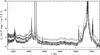 |
Fig. 1 HET spectra of Mrk 926 taken between August 3 and December 6, 2005. The wavelength ranges for the Hβ and Hα lines as well as for the optical continua are indicated at the bottom (see Table 2). |
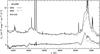 |
Fig. 2 Mean spectra of Mrk 926 taken in the years 2004 (solid line) and 2005 (dash-dotted line). The difference spectrum between the two observing campaigns is shown at the bottom (dotted line). It has been scaled by a factor of 2 (solid line) to enhance the contrast between features. |
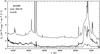 |
Fig. 3 Integrated mean spectrum of Mrk 926 for the years 2004 and 2005. The rms spectrum is given at the bottom. This spectrum has been scaled by a factor of 6 (zero level is shifted by –1.5) to enhance weaker line structures. |
Two general results are immediately evident: the continuum flux was bluer in 2005 than in 2004, while the mean flux at 6000 Å was almost equal at both epochs. The second trend is related to general profile changes in the Balmer lines Hγ, Hβ, and Hα. The outer blue wings are stronger in 2005 than in 2004 – seen as absorption troughs in the difference spectra – while the remaining blue wings as well as the red wings show the opposite trend. This trend is unequally pronounced in the different Balmer lines. The Hα line shows the strongest variations. The double peaked Hα profile is also clearly distinctive in the difference spectrum. The line variations are discussed later in the context of the line profiles.
Figure 3 shows the mean spectrum of Mrk 926 for both campaigns in 2004 and 2005. The rms spectrum is given at the bottom with two different vertical scalings. It has in addition been scaled by a factor of 6 (zero level is shifted by –1.5) to enhance weaker line structures. The rms spectra show the variable parts of the line profiles. Besides an inner double-peaked profile – as seen in the difference Hα spectrum – two separate outer blue and red components are visible in the Hα and Hβ rms spectra. These spectra are also discussed later in the context of the line profiles.
We inspected the spectra for continuum regions that are free of both strong emission and absorption lines. Because of the extreme line widths of the broad emission line profiles in Mrk 926, it is difficult to confine these regions. We finally identified four continuum regions close to 4600, 5180, 5500, and 6200 Å (see Table 2),
Boundaries of mean continuum values and line integration limits.
3.2. Continuum and emission-line light curves
It is important to identify wavelength ranges in AGN spectra that are free of both emission and absorption lines to derive their continuum light curves. The continuum region at 5100 Å has widely been used in studies of many AGNs, such as the prototype Seyfert galaxy NGC 5548 (Peterson et al. 1992). The spectral range between 5130 and 5140 Å was found to be a more appropriate continuum region in the narrow-line Seyfert galaxy Mrk 110 (Kollatschny et al. 2003). However, because of the extreme Hβ line width (see Fig. 2) of Mrk 926 the most appropriate continuum section is the wavelength interval 5170–5183 Å. Three additional optical continuum ranges were selected close to 4600 Å, 5500 Å, and 6200 Å (see Table 2).
We integrated the broad emission-line intensities of Hβ and Hα, between the boundaries listed in Table 2. Figure 1 shows the selected wavelength ranges for the Hβ and Hα lines as well as for their related optical continuum ranges.
We first subtracted a linear pseudo-continuum defined by the boundaries given in Table 2. For the Hα line, we found only one continuum data point only on the blue side of this line. For our intensity measurements, we assumed that the continuum is flat below Hα. Constant narrow line components were subtracted first before we measured the broad line intensities. The results of the continuum and line intensity measurements are given in Table 3.
Continuum and integrated line fluxes.
We derived a mean continuum flux of Fλ(5180 Å) = 2.82 ± 0.23 × 10⁻¹⁵ erg s-1 cm-2 Å-1 (from Table 3) at 5180Å for 2005. This corresponds to a mean luminosity of L(5180 Å) = 1.159 ± 0.094 × 1040 erg s-1 Å-1 or λ Lλ(5180 Å) = 5.91 ± 0.56 × 1043 erg s-1. The mean Hβ flux amounts to F(Hβ) = 3.87 ± 0.39 × 10⁻¹³ erg s-1 cm-2, and the mean Hβ luminosity to L(Hβ) = 1.59 ± 0.16 × 1042 erg s-1 Å-1. In Fig. 4 we present the light curves of the continuum fluxes at 4600 and 5180 Å (in units of 10-15 erg cm-2 s-1 Å-1) and the light curves of the integrated emission-line fluxes of Hβ and Hα for both campaigns performed in 2004 and 2005 and in greater detail for 2005 (right column). Conspicuous variability amplitudes in the continuum as well as in the emission line fluxes are to be seen on timescales of a few days only.
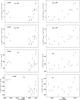 |
Fig. 4 Light curves of the continuum fluxes at 4600 and 5180 Å (in units of 10-15 erg cm-2 s-1 Å-1) and of the integrated emission line fluxes of Hβ and Hα (in units of 10-15 erg cm-2 s-1) for the years 2004 and 2005 and in greater detail for the year 2005 (right column). |
as defined by Rodríguez-Pascual et al. (1997).
Variability statistics for Mrk 926 in the year 2005 (upper half) as well as for both years 2004/2005 (lower half).
3.3. Difference line profiles
Figure 5 shows the difference line profiles of Hα (dashed line), Hβ (solid line), and Hγ (dotted line) in velocity space for the two observing campaigns in the years 2004 and 2005.
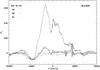 |
Fig. 5 Difference line profiles of Hα (dashed line), Hβ (solid line), and Hγ (dotted line) in velocity space for the two campaigns in 2004 and 2005. |
The difference spectra of Hα, Hβ, and Hγ have common characteristics. An additional intensity trend is superimposed decreasing from Hα to Hγ: both Hα and Hβ show double-peaked profiles with two separate broad components centered at –3400 ± 200 and –1500 ± 200 km s-1. These two components are not located symmetrically with respect to v = 0 km s-1. The blue line component is stronger than the red one indicating that there are stronger variations in the blue rather than the red wing. Furthermore, all three difference spectra show a broad minimum of identical intensity at –9000 ± 500 km s-1. This is the only section in all Balmer line profiles where the 2004 spectra were more intense than the 2005 spectra.
The relative strengths of the difference line intensities with respect to their corresponding mean line intensities are different for the three Balmer lines (see Fig. 2). The intensity of the Hα difference spectrum (between v = −17 000, +19 000 km s-1) corresponds to 20% of the Hα mean spectrum. However, the intensity of the Hβ difference spectrum is small compared to the mean Hβ spectrum, i.e., 0.5% or rather 5% when considering the positive fraction of the difference spectrum only.
3.4. Mean line profiles
Normalized mean and rms line profiles of Hα and Hβ are presented in Figs. 6 to 10 in velocity space. The mean Hα and Hβ profiles are free of any detailed structures (Fig. 6).
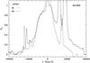 |
Fig. 6 Normalized mean line profiles of Hα (dashed line) and Hβ (solid line). |
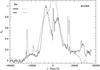 |
Fig. 7 Normalized mean (dashed line) and rms (solid line) line profiles of Hα in velocity space. |
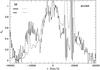 |
Fig. 8 Normalized mean (dashed line) and rms (solid line) line profiles of Hβ in velocity space. |
 |
Fig. 9 Normalized rms line profiles of Hα (dashed line) and Hβ (solid line) in velocity space. |
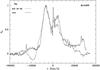 |
Fig. 10 Normalized rms (solid line) and difference (dashed line) line profiles of Hα in velocity space. |
3.5. Rms line profiles
The rms spectra illustrate the variations in the line profile segments during our variability campaign in the years 2004 and 2005. Our rms profiles (Figs. 7–9) consist of five distinguishable components: a narrow central component, two broad inner blue and red wing components, and two even broader outer wing components. The intervals of the individual rms line segments are given in Table 5.
Intervals of the Hβ and Hα line-profile segments.
The outer wing components in Hα and Hβ are broader than the inner wing components. The relative intensities of the outer components with respect to the inner ones are different for the Hα and Hβ lines, i.e., the outer blue component is far stronger in Hβ than in Hα (Fig. 9). This causes a shift in the dividing line between outer and inner blue component in Hβ. Therefore, at least some of the different line segment limits in Hα and Hβ might be caused by the relative intensities of the line segments. The maxima of the outer blue components of Hα and Hβ are at –9500 km s-1 in both profiles. One may suspect that the strong outer blue component in the Hβ rms profile is caused by a blend with a variable underlying He ii λ4686 line (see Fig. 10), as seen in Mrk 110 (Kollatschny et al. 2001). However, this is less likely to be true for Mrk 926: the He ii λ4686 line is centered on –10 800 km s-1 but the observed outer blue wing is centered on –9500 km s-1 (Fig. 8).
The blue-to-red intensity ratios of the inner line components in the rms profiles are different for Hα and Hβ (Fig. 9), the inner blue component in Hα being stronger than the red component, and the opposite being true for Hβ. Comparing the line profiles and the widths of the inner Hα components in the rms profile with those in the difference profile (see Fig. 10) indicates that they are very similar, in contrast to the case for the outer components.
The Balmer line profiles in Mrk 926 are extremely broad (see Figs. 8, 9). We derived line-widths (FWHM) of between 8520 and 11 920 km s-1 from the mean and rms line profiles (Table 6). Furthermore, we parameterized the line widths of the rms profiles by their line dispersions σline (rms widths) (Fromerth & Mellia 2000, Peterson et al. 2004). The measured Balmer line dispersions σline of more than 7000 km s-1 (Table 6) are also indicative of very broad line widths. The red wing of the Hβ mean profile is heavily blended with the [O iii] lines leading to a large uncertainty. The full widths at zero intensity (FWZI) in the Balmer lines even correspond to 35 000 km s-1.
Balmer line widths: FWHM of the mean and rms line profiles as well as line dispersion σline (rms width) of the rms profiles.
3.6. CCF and DCF analysis
The size of the broad emission-line region in AGN can be estimated by evaluating of the cross-correlation function (CCF) of the ionizing continuum flux light curve with the light curves of the variable broad emission lines. An interpolation cross-correlation function method (ICCF) was developed by Gaskell & Peterson (1987). An independent method is the discrete correlation function (DCF) method described by Edelson & Krolik (1988). Based on these papers, we developed our own ICCF and DCF code (Dietrich & Kollatschny 1995).
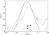 |
Fig. 11 Cross-correlation functions CCF(τ) of the continuum light curve at 5180 Å with the Hβ and Hα light curves as well as the Hβ auto-correlation function. |
We cross-correlated the individual continuum light curves of Mrk 926 with both the other continuum light curves and the light curves of the integrated Hβ and Hα lines using the ICCF method. Furthermore, we correlated the Hβ light curve with itself (evaluating the auto-correlation function). Figures 11–13 show the cross-correlation functions CCF(τ) of the continuum light curve at 5180 Å with the Balmer line light curves and the Hβ auto-correlation function (ACF).
We used the inner part within ± 6000 km s-1 only for the integrated Hβ line neglecting the outer line wings. The outer blue line wing of Hβ seems to be contaminated with He ii λ4686. We derived the cross-correlation function of the Hα line for the same inner line profile segment to compare these lines with each other.
The width of the Hβ auto-correlation function provides an indication of the BLR size (e.g. Gaskell & Peterson 1987). The Hβ ACF shows that the BLR radius is smaller than 15–20 light-days indicating that the BLR in Mrk 926 is small. Spatially resolved velocity delay maps of Hβ and Hα are discussed in Sect. 4.
We independently tested our ICCF results by calculating the discrete correlation functions. The results of the discrete correlation functions for Hβ and Hα (crosses with error bars) obtained with a binning of 5 days are presented in Figs. 12 and 13. For comparison, we present in Figs. 12 and 13 the cross-correlation functions CCF(τ) of the integrated Hβ and Hα light curves (solid lines). The discrete correlation functions confirm the trend of a very small BLR.
The centroids of the ICCF, τcent, were calculated using only the part of the CCF above 90% of the peak value. We derived the uncertainties in the cross-correlation results by calculating the cross-correlation lags a large number of times using a model-independent Monte Carlo method known as “flux redistribution/random subset selection” (FR/RSS), a method described by Peterson et al. (1998b). The error intervals correspond to 68% confidence levels.
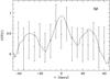 |
Fig. 12 Cross-correlation function CCF(τ) (solid line) and DCF (error bars) of the Hβ light curve with the 5180 Å continuum light curve. |
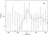 |
Fig. 13 Cross-correlation function CCF(τ) (solid line) and DCF (error bars) of the Hα light curve with the 5180 Å continuum light curve. |
The final results of the ICCF analysis are given in Table 7.
Cross-correlation lags of the continuum light curve at 4600 Å and of the Balmer-line light curves with respect to the 5180 Å continuum.
 light-days
only. The delay of the integrated Hα line corresponds to
light-days
only. The delay of the integrated Hα line corresponds to
 light-days only.
The derived lags may be equal zero within the errors indicating that we have derived at
least an upper limit to the BLR size in Mrk 926.
light-days only.
The derived lags may be equal zero within the errors indicating that we have derived at
least an upper limit to the BLR size in Mrk 926.
The broad-line region size in Mrk 926 we derived from the Balmer lines is small compared to those in other Seyfert galaxies (for comparison see Kaspi et al. 2005). This is reviewed in more detail in the discussion section.
3.7. Central black hole mass
The central black hole mass in Mrk 926 can be derived from the width of the broad emission line profiles based on the assumption that the gas dynamics are dominated by the central massive object, by evaluating M = fcτcentΔv2G-1. The characteristic distance of the line-emitting region τcent is given by the centroid of the individual cross-correlation functions of the emission-line variations relative to the continuum variations (e.g. Koratkar & Gaskell 1991; Kollatschny & Dietrich 1997). We derived upper limits to the Hβ and Hα cross-correlation lags τcent based on the delay of the emission-line light curves with respect to the continuum light curve at 5180 Å since a significant lag was not detected.
The characteristic velocity Δv of the emission-line region can be estimated from either the FWHM of the rms profile or from the line dispersion σline. We wish to compare the central black hole mass in Mrk 926 with the central black hole masses of other AGN in the database of Peterson et al. (2004). Therefore, we used the line dispersion σline to calculate the central black hole mass in Mrk 926.
The scaling factor f in the equation above is of the order of unity and depends on the kinematics, structure, and orientation of the BLR. The scaling factor may differ from galaxy to galaxy e.g. if we see the central accretion disk including the BLR from the edge or face-on. Again we recall that we wish to compare the central black hole mass in Mrk 926 with the central masses in the AGN sample of Peterson et al. (2004), and therefore, we adopt their mean value of f = 5.5.
In Table 8, we list our virial mass calculations of the central black hole in Mrk 926 based on the Balmer lines.
Line dispersion σline (rms width) of the rms Balmer profiles, upper limits of the Hβ and Hα emission line cross-correlations, and derived central black hole mass limits.

Based on Hβ and Hα, we derive a weighted average limit of

for Mrk 926.
4. 2-D CCF of the Hα and Hβ line profiles
We now investigate in detail the line profile variations of Hα and Hβ. We proceed in the same way as when we studied the line profile variations in Mrk 110 (Kollatschny & Bischoff 2002; Kollatschny 2003).
We sliced the Hα and Hβ velocity profiles into velocity segments of widths Δv = 400 km s-1 for all the spectra taken in 2005. The value of 400 km s-1 corresponds to the spectral resolution of our observations. We measured the intensities of all subsequent velocity segments from v = −15 000 until +15 000 km s-1 and compiled their light curves. The intensity of the central line segment was integrated from v = −200 until +200 km s-1.
All the light curves of the line segments including the light curves of the continuum at 5180 Å look similar. There are no clear-cut differences between the outer and inner segments or between the red and blue wings. We computed cross-correlation functions (CCFs) of all line segment (Δv = 400 km s-1) light curves with the 5180 Å continuum light curve.
The derived delays of the segments with respect to the 5180 Å continuum light curve are shown in Figs. 14 and 15 as a function of distance to the line center.
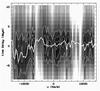 |
Fig. 14 The 2-D CCF(τ,v) shows the correlation of the Hβ line segment light curves with the continuum light curve at 5180 Å as a function of velocity and time delay (grey scale). Contours of the correlation coefficient are overplotted at levels of 0.93, 0.89, and 0.80 (solid lines). The heavy dashed line connects the centers of all individual cross-correlation functions. |
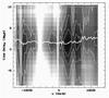 |
Fig. 15 The 2-D CCF(τ, v) shows the correlation of the Hα line segment light curves with the continuum light curve at 5180 Å as a function of velocity and time delay (grey scale). Contours of the correlation coefficient are overplotted at levels of 0.85, 0.75, and 0.65 (solid lines). The heavy dashed line connects the centers of all individual cross-correlation functions. |
The thin solid lines of Figs. 14 and 15 delineate the contour lines of the correlation coefficient at levels of .93, .89, and .75 for Hβ and at levels of .85, .75, and .65 for Hα. The heavy dashed line connects the centers of all cross-correlation functions for the different line profile segments. The time delay of the line segment light curves was calculated from the uppermost 10 percent of the cross-correlation functions. Only correlation coefficients with values greater than .6 were considered for Hβ.
Figure 16 shows the delay of the individual line segments together for both lines Hα and Hβ; these delays correspond to the heavy dashed lines in Figs. 14 and 15.
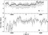 |
Fig. 16 Time delay of the individual line segments of Hα (solid line, filled square) and Hβ (dashed line, open circle) with respect to the continuum light curve at 5180 Å. |
Both lines (Hα and Hβ) respond with very short delays relative to the continuum at 5180 Å as derived previously from the integrated lines. Within the small-scale variations, they are nearly constant along the line profile with one exception: There is a drop in the delay of the outer blue wing of Hβ between v = −14 000 and −8400 km s-1. This wavelength range corresponds exactly to the He ii λ4686 line centered on –10 800 km s-1. It is known from other galaxies (e.g. Mrk 110, Kollatschny et al. 2001) that the He ii λ4686 line exhibits shorter delays with respect to the ionizing continuum than the Hβ line. The apparent negative delay of two light-days with respect to the continuum light curve at 5180 Å might be caused by a general systematic error or by an alternative possibility that the continuum flux at 5180 Å does not correspond to the ionizing continuum flux.
Figure 17 shows the response of the Hα and Hβ line segment cross-correlation functions.
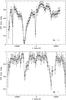 |
Fig. 17 Maximum response of the correlation functions of the Hα (solid line, filled square) and Hβ (dashed line, open circle) line segment light curves with the continuum light curve at 5180 Å. |
Intervals of the response segments derived from the 2-D CCFs of Hβ and Hα.
5. Discussion
Mrk 926 is a very broad-line Seyfert 1 galaxy. It remains unclear the extent to which the extreme emission line-widths in the individual very broad-line AGN are caused by intrinsic properties of the galaxy or by projection effects of the central BLR accretion disk.
5.1. Mean and rms line-profiles in Mrk 926
The mean and the rms Balmer lines in Mrk 926 are extremely broad. They have full width half maxima (FWHM) of the order of 10 000 km s-1 (Figs. 7 and 8). The full width at zero intensity (FWZI) of Hβ amounts to 35 000 km s-1.
It was noted by Fromerth & Mellia (2000) and Peterson et al. (2004) that an emission line width can be parameterized by their FWHM and their line dispersion σline. We derived a line dispersion σline of 7100 km s-1 for the Balmer lines in Mrk 926. No other galaxy in the sample of 35 AGN (Peterson et al. 2004) exhibits such a broad line dispersion σline. In terms of the FWHM, only 3C 390.3 shows broader wings than Mrk 926.
For a Gaussian line profile, the ratio FWHM/σline is 2.355. Peterson et al. (2004) derived a mean ratio of FWHM/σline = 2.03 in their sample indicating that their emission lines had in general weaker cores and stronger wings than Gaussian profiles. We derived an extreme FWHM/σline ratio of 1.2 only for Mrk 926 based on the rms Balmer profiles. This ratio confirms the existence of the very strong line wings seen in Fig. 9. Only five AGNs in the sample of Peterson et al. (2004) have similar ratios of FWHM/σline ≤ 1.2 for Hβ (their Table 6, Fig. 9).
The rms profiles in Mrk 926 are more complex than one would expect if they were formed in a basic optically thin accretion disk. A simple accretion disk would produce a double-peaked profile (e.g. Welsh & Horne 1991; Horne et al. 2004), although this simple model cannot easily explain the existence of two inner and two outer line components in addition to a central component. Furthermore, the components are not arranged symmetrically with respect to v = 0 km s-1. In a few other broad-line galaxies (3C 390.3, 3C 332), similar complex structures have been found in the rms profiles (Gezari et al. 2007). The geometrical and physical conditions causing these complex profiles are not yet fully understood.
The different behaviour of the line components in Hα and Hβ (Figs. 6 to 9) indicates that the components might originate in different regions or in regions of different optical thickness. The segmented structure in the line profiles will be addressed again in conjunction with the two-dimensional cross-correlation function (Sect. 5.4).
5.2. The BLR size in Mrk 926
We correlated the individual continuum light curves of Mrk 926 with each other and with the Balmer emission-line light curves. Figures 11 to 13 and Table 7 display the delays of the Balmer lines with respect to the continuum light curve at 5180 Å and the Hβ auto-correlation function.
Mrk 926 has a very small BLR. This is based on the Hβ auto-correlation
function as well as on the delays of the Balmer line light curves with respect to the
continuum light curve at 5100 Å. We determined a line-averaged Hβ BLR
size of light-days and
a Hα BLR size of light-days. The
upper limit of 2 light-days to the Hβ BLR size in Mrk 926 corresponds to
the smallest BLR sizes in the AGN sample of Kaspi et al. (2005). They investigated the relationship between AGN luminosity and broad-line
size on the basis of the most accurate determinations of BLR radii for 35 AGNs (their
Fig. 2). Mrk 926 deviates slightly from the general
relationship between luminosity and broad-line region size in AGNs. However, other
broad-line Seyfert galaxies of comparable luminosity e.g. IC 4329A, NGC 7469, and NGC 4593
also exhibit similar deviations from the general trend.
From the general relation of Kaspi et al. (2005), one would predict a larger BLR size of Mrk 926 with respect to the measured continuum luminosity. A continuum luminosity of λLλ(5100Å) = 5.91 ± 0.56 × 1043 erg s-1 corresponds to a seven times larger BLR size of R(BLR) = 15.51 light-days using Eq. (6) of Kaspi et al. (2005). Such a large BLR size can be excluded by the auto-correlation and cross-correlation functions.
There is the possibility that the derived small delay for the Balmer-line emitting region does not correspond to the true distance of the line-emitting region from the central ionizing source. This distance might be larger by the order of two to four light-days because of the possibility that the observed continuum at 5180 Å does not correspond to the ionizing continuum in the UV below 1000 Å. Evidence of a wavelength-dependent continuum delay in the optical was found in the Seyfert galaxy NGC 7469 (Wanders et al. 1997, Collier et al. 1998). These observations were interpreted as reprocessing of high-energy radiation close to the center in an irradiated black-body accretion disk with a T ∝ R−4/3 temperature profile, which causes delays of τ ∝ λ4/3. Sergeev et al. (2005) published wavelength-dependent continuum delays based on broad-band photometry of the light curves of 14 AGN. They interpreted their observations in terms of reprocessed emission of an X-ray source above the accretion disk. Gaskell (2007, 2008) explained the observed wavelength-dependent continuum delays as possibly being caused by contamination of an intrinsically coherently variable continuum with the Wien tail of the thermal emission from the hot dust in the surrounding torus. The detection of a lag in the polarized flux provides a way to discriminate between both models.
5.3. Central black hole mass in Mrk 926
We derived an upper limit of M = 11.2 × 10⁷ M⊙ to the central black hole mass based on both the distance of the Hβ line-emitting region and the line dispersion σline of the rms line profile. Peterson et al. (2004) presented a black hole mass-luminosity relationship for 35 reverberation mapped AGNs. With respect to its optical luminosity, the black hole mass of Mrk 926 is within the expected range of a few times 107 M⊙ (their Fig. 16).
An estimate of the black hole mass based on the line width alone is less reliable. From the line widths of Mrk 926, O’Neill et al. (2005) derived a very high black hole mass of 3.5 × 10⁸ M⊙ and compared this number with the observed X-ray variability amplitude observed by ASCA. But they derived only an upper limit to their excess variance (see their Fig. 2). Since the intrinsic black hole mass in Mrk 926 is lower by a factor of three, one would expect a slightly more variable X-ray source.
5.4. 2D velocity map
The delays of the individual line segments of Hα and Hβ with respect to the continuum variability at 5180 Å are very short (0 to 3 light-days only) and more or less constant over the entire line profile (Figs. 14 to 16). There is a drop in the outer blue wing of Hβ between v = −14 000 and –8400 km s-1. This line region corresponds to a blend of the He ii λ4686 line in the blue wing of Hβ. The He ii λ4686 line is centered on –10 800 km s-1 with respect to Hβ. The Hα line does not show this drop in the blue wing.
The computed delay of the He ii λ4686 line is negative with respect to the continuum at 5180 Å by about two light days. This negative delay is within our systematic error of three light-days. Another explanation of the negative delay is the possibility that the optical continuum light curve at 5180 Å does not correspond to the ionizing continuum of the He ii λ4686 line in the far-UV because of a wavelength-dependent continuum delay. Spectral observations on a daily basis are needed to solve this question that the He ii λ4686 line originates in the innermost region while the Hα line originates in more exterior regions than Hβ as has been found e.g. in Mrk 110 (Kollatschny et al. 2001) too.
Figures 14 and 15 show the 2-D cross-correlation functions CCF(τ, v) of the Hβ and Hα line segment light curves with the continuum light curve at 5180 Å as a function of velocity and time delay (grey scale). These 2-D CCF(τ, v) are mathematically very similar to a 2-D response function Ψ (Welsh 2001). We compare our observed velocity-delay pattern with model calculations of Welsh & Horne (1991), Perez et al. (1992), O’Brien et al. (1994), Horne et al. (2004), and with results of Mrk 110 (Kollatschny 2003).
The delay in the individual line segments is very small. We could not discern any trend as a function of distance to the line center except for the drop in the blue Hβ wing. The observed uniformity of the line-segment delays in Mrk 926 is different from that observed in Mrk 110 (Kollatschny 2003). In that galaxy, the emission line wings responded far more quickly than the central line region. Their central Balmer line regions responded with a delay of about 30 light days with respect to the ionizing continuum. However, an existing pattern might be hidden in the 2-D CCFs of Mrk 926 due to the very small BLR. Our temporal sampling is insufficient to detect any detailed pattern on timescales shorter than about three light-days.
The observed emission lines and their corresponding 2-D CCFs are very broad. The line widths of Mrk 926 amount to 10 000 km s-1 (FWHM) compared to line widths of 2000 km s-1 only in Mrk 110 (Kollatschny et al. 2001). It has been demonstrated that the narrow Balmer and helium emission lines in Mrk 110 originate in an accretion disk seen nearly face on (Kollatschny 2002, 2003). The response of the very broad emission lines in Mrk 926 might be caused by an accretion disk seen nearly edge on relative to e.g. the model calculations of Perez et al. (1992, their Fig. 6) or Welsh & Horne (1991, their Fig. 5).
Figure 18 shows the response of the Hα and Hβ line segment cross-correlation functions as well as their normalized rms profiles in one plot. The response curves have been shifted by 0.5 to avoid any strong overlap of the curves. Furthermore, two spikes in the [OIII] residuals have been removed.
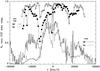 |
Fig. 18 Maximum response of the correlation functions of the Hα (solid line, filled square) and Hβ (dashed line, open circle) line segment light curves with the continuum light curve at 5180 Å as well as their normalized rms profiles. The response curves are shifted by 0.5 to avoid strong overlap of the curves. |
The response of the (inner) red wing is stronger than the response of the (inner) blue wing (Figs. 14, 15, and 17). The stronger response of the red line wing relative to the blue line wing was predicted by Chiang & Murray (1996) in their accretion disk-wind model of the BLR. Similar evidence of an accretion disk wind was detected in Mrk 110 ( Kollatschny 2003). The response of the outer line wings (shortwards of −6000 km s-1 and longwards of 8000 km s-1) does not follow this trend. The outer line wings might originate from different physical conditions.
A structured response may be considered as independent evidence of a structured BLR: the broad emission lines may then originate in a homogeneous medium or different line segments may originate in different regions and/or under different physical conditions.
6. Summary
A spectroscopic monitoring campaign of the very broad line AGN Mrk 926 was carried out by ourselves with the 9.2 m Hobby-Eberly Telescope in the years 2004 and 2005. The main results of our study can be summarized as follows:
-
1.
The rms profiles of the very broad Balmer lines (10 000 km s-1FWHM) are structured showing two inner and two outer line components in addition to a central component. The outer and inner line segments vary with different amplitudes.
-
2.
The radius of the BLR is quite small with an upper limit of 2 light-days for the Hβ BLR size.
-
3.
We calculated an upper limit of M = 11.2 × 10⁷ M⊙ for the central black hole mass in Mrk 926. This result was based on the Hβ line dispersion σline and the upper limit to the cross-correlation lag τcent. The central black hole mass in Mrk 926 is inside the expected range of a few times 107 M⊙ with respect to its optical luminosity.
-
4.
The 2-D cross-correlation functions CCF(τ, v) of Hβ and Hα are flat within the error limits. However, the response of the Balmer line segments is structured. A double structure in the Hα and Hβ response curves – showing two separate inner and outer components – has also been seen in the rms line profiles. The different line segments might originate in separate regions and/or under different physical conditions.
Acknowledgments
We thank Shai Kaspi and Martin Gaskell for useful comments. This work has been supported by the Niedersachsen – Israel Research Cooperation Program ZN2318.
References
- Bentz, M. C.,Walsh, J. L.,Barth, A. J., et al. 2008, ApJ, 689, L21 [NASA ADS] [CrossRef] [Google Scholar]
- Bentz, M. C.,Walsh, J. L.,Barth, A. J., et al. 2009, ApJ, 705, 199 [NASA ADS] [CrossRef] [Google Scholar]
- Chiang, J., & Murray, N. 1996, ApJ, 466, 704 [NASA ADS] [CrossRef] [Google Scholar]
- Collier, S. J.,Horne, K.,Kaspi, S., et al. 1998, ApJ, 500, 162 [NASA ADS] [CrossRef] [Google Scholar]
- Denney, K. D.,Peterson, B. M.,Pogge, R. W., et al. 2009, ApJ, 704, L80 [NASA ADS] [CrossRef] [Google Scholar]
- Dietrich, M., & Kollatschny, W. 1995, A&A, 303, 405 [NASA ADS] [Google Scholar]
- Dietrich, M.,Kollatschny, W.,Peterson, B. M., et al. 1993, ApJ, 408, 416 [NASA ADS] [CrossRef] [Google Scholar]
- Doroshenko, V. T.,Sergeev, S. G., & Pronik, V. I. 2008, Astron. Rep., 52, 442 [NASA ADS] [CrossRef] [Google Scholar]
- Durret, F., & Bergeron, J. 1988, A&AS, 75, 273 [Google Scholar]
- Edelson, R. A., & Krolik, J. H. 1988, ApJ, 333, 646 [NASA ADS] [CrossRef] [Google Scholar]
- Fromerth, M. J., & Melia, F. 2000, ApJ, 533, 172 [NASA ADS] [CrossRef] [Google Scholar]
- Garnier, R.,Paturel, G.,Petit, C., et al. 1996, A&AS, 117, 467 [Google Scholar]
- Gaskell, C. M., & Peterson, B. M. 1987, ApJS 65, [Google Scholar]
- Gaskell, C. M. 2007, in The Central Engine of Active Galactic Nuclei, ed. Luis C. Ho, & Jian-Min Wang, ASP Conf. Ser., 373, 596 [Google Scholar]
- Gaskell, C. M. 2008, in The Nuclear Region, Host Galaxy and Environment of Active Galaxies, eds. E. Benitez, I. Cruz-Gonzalez, & Y. Krongold, Rev. Mex. Astron. y Astrofisi. Ser. Conf. 32, 1 [Google Scholar]
- Gezari, S., Halpern, J. P., & Eracleous, M. 2007, ApJS 169, 167 [NASA ADS] [CrossRef] [Google Scholar]
- Horne, K., Peterson, B. M., Collier, S. J., et al. 2004, PASP 116, 465 [NASA ADS] [CrossRef] [Google Scholar]
- Kaspi, S., Maoz, D., Netzer, H., et al. 2005, ApJ 629, 61 [NASA ADS] [CrossRef] [Google Scholar]
- Kollatschny, W. 2003, A&A, 407, 461 [NASA ADS] [CrossRef] [EDP Sciences] [Google Scholar]
- Kollatschny, W., & Bischoff, K. 2002, A&A, 386, L19 [NASA ADS] [CrossRef] [EDP Sciences] [Google Scholar]
- Kollatschny, W., & Dietrich, M. 1997, A&A, 323, 5 [NASA ADS] [Google Scholar]
- Kollatschny, W., & Fricke, K. J. 1985, A&A, 146, L11 [NASA ADS] [Google Scholar]
- Kollatschny, W.,Fricke, K. J.,Schleicher, H., & Yorke, H. W. 1981, A&A, 102, L23 [NASA ADS] [Google Scholar]
- Kollatschny, W.,Bischoff, K., & Dietrich, M. 2000, A&A, 361, 901 [NASA ADS] [Google Scholar]
- Kollatschny, W.,Bischoff, K.,Robinson, E. L., et al. 2001, A&A, 379, 125 [NASA ADS] [CrossRef] [EDP Sciences] [Google Scholar]
- Kollatschny, W.,Zetzl, M., & Dietrich, M. 2006, A&A, 454, 459 [NASA ADS] [CrossRef] [EDP Sciences] [Google Scholar]
- Koratkar, A., & Gaskell, M. 1991, ApJ 370, L61 [NASA ADS] [CrossRef] [Google Scholar]
- Kuehn, C. A.,Baldwin, J. A.,Peterson, B. M., et al. 2008, ApJ, 673, 69 [NASA ADS] [CrossRef] [Google Scholar]
- Marziani, P.,Sulentic, J. W.,Calvani, M., et al. 1993, ApJ, 410, 56 [NASA ADS] [CrossRef] [Google Scholar]
- Morris, S. L., & Ward, M. J. 1988, MNRAS, 230, 639 [NASA ADS] [CrossRef] [Google Scholar]
- O’Brien, P. T., Goad, M. R., & Gondhalekar, P. M., 1994, MNRAS, 268, 845 [NASA ADS] [CrossRef] [Google Scholar]
- O’Neill, P. M., Nandra, K., Papadakis I. E., et al. 2005, MNRAS, 358, 1405 [NASA ADS] [CrossRef] [Google Scholar]
- Osterbrock, D. E. 1977, ApJ, 215, 733 [NASA ADS] [CrossRef] [Google Scholar]
- Osterbrock, D. E., & Shuder, J. M. 1982, ApJS, 49, 149 [NASA ADS] [CrossRef] [Google Scholar]
- Perez, E.,Robinson, A., & de la Fuente, L. 1992, MNRAS, 256, 103 [NASA ADS] [CrossRef] [Google Scholar]
- Penston, M. V., & Perez, E. 1984, MNRAS, 211, 33 [Google Scholar]
- Peterson, B. M.,Alloin, D.,Axon, D., et al. 1992, ApJ, 392, 470 [NASA ADS] [CrossRef] [Google Scholar]
- Peterson, B. M.,Wanders, I., & Bertram, R. 1998a, ApJ, 501, 82 [NASA ADS] [CrossRef] [Google Scholar]
- Peterson, B. M.,Wanders, I.,Horne, K., et al. 1998b, PASP, 110, 660 [NASA ADS] [CrossRef] [Google Scholar]
- Peterson, B. M., Berlind, P., Bertram, R. et al. 2002, ApJ, 581, 197 [NASA ADS] [CrossRef] [Google Scholar]
- Peterson, B. M.,Ferrarese, L.,Gilbert, K. M., et al. 2004, ApJ, 613, 682 [NASA ADS] [CrossRef] [Google Scholar]
- Rodríguez-Pascual P. M., Alloin D., Clavel J., et al., 1997, ApJS 110, 9 [NASA ADS] [CrossRef] [Google Scholar]
- Sergeev, S. G.,Pronik, V. I., & Sergeeva, E. A. 2001, ApJ, 554, 245 [NASA ADS] [CrossRef] [Google Scholar]
- Sergeev, S. G.,Pronik, V. I.,Peterson, B. M., et al. 2002, ApJ, 576, 660 [NASA ADS] [CrossRef] [Google Scholar]
- Sergeev, S. G.,Doroshenko, V. T.,Golubinskiy, Yu. V., et al. 2005, ApJ, 622, 129 [NASA ADS] [CrossRef] [Google Scholar]
- Sergeev, S. G., Doroshenko, V. T., Dzyuba, S. A. et al. 2007, ApJ, 668, 708 [NASA ADS] [CrossRef] [Google Scholar]
- Storchi-Bergmann, T., Nemmen da Silva, R., Eracleous, M. et al. 2003, ApJ, 598, 956 [NASA ADS] [CrossRef] [Google Scholar]
- Wanders, I., Peterson, B. M., Alloin, et al. 1997, ApJS, 113, 69 [NASA ADS] [CrossRef] [Google Scholar]
- Wang, J.,Wei, J. Y., & He, X. T. 2005, A&A, 436, 417 [NASA ADS] [CrossRef] [EDP Sciences] [Google Scholar]
- Ward, M. J., Wilson, A. S., Penston, M. V., et al., 1978, ApJ., 223, 788 [NASA ADS] [CrossRef] [Google Scholar]
- Welsh, W. F., & Horne, K. 1991, ApJ, 379, 586 [NASA ADS] [CrossRef] [Google Scholar]
- Welsh, W. F. 2001, in Probing the Physics of AGN, ed. Peterson et al., ASP Conf. Ser., 224, 123 [Google Scholar]
All Tables
Variability statistics for Mrk 926 in the year 2005 (upper half) as well as for both years 2004/2005 (lower half).
Balmer line widths: FWHM of the mean and rms line profiles as well as line dispersion σline (rms width) of the rms profiles.
Cross-correlation lags of the continuum light curve at 4600 Å and of the Balmer-line light curves with respect to the 5180 Å continuum.
Line dispersion σline (rms width) of the rms Balmer profiles, upper limits of the Hβ and Hα emission line cross-correlations, and derived central black hole mass limits.
All Figures
|
Fig. 1 HET spectra of Mrk 926 taken between August 3 and December 6, 2005. The wavelength ranges for the Hβ and Hα lines as well as for the optical continua are indicated at the bottom (see Table 2). |
| In the text | |
|
Fig. 2 Mean spectra of Mrk 926 taken in the years 2004 (solid line) and 2005 (dash-dotted line). The difference spectrum between the two observing campaigns is shown at the bottom (dotted line). It has been scaled by a factor of 2 (solid line) to enhance the contrast between features. |
| In the text | |
|
Fig. 3 Integrated mean spectrum of Mrk 926 for the years 2004 and 2005. The rms spectrum is given at the bottom. This spectrum has been scaled by a factor of 6 (zero level is shifted by –1.5) to enhance weaker line structures. |
| In the text | |
|
Fig. 4 Light curves of the continuum fluxes at 4600 and 5180 Å (in units of 10-15 erg cm-2 s-1 Å-1) and of the integrated emission line fluxes of Hβ and Hα (in units of 10-15 erg cm-2 s-1) for the years 2004 and 2005 and in greater detail for the year 2005 (right column). |
| In the text | |
|
Fig. 5 Difference line profiles of Hα (dashed line), Hβ (solid line), and Hγ (dotted line) in velocity space for the two campaigns in 2004 and 2005. |
| In the text | |
|
Fig. 6 Normalized mean line profiles of Hα (dashed line) and Hβ (solid line). |
| In the text | |
|
Fig. 7 Normalized mean (dashed line) and rms (solid line) line profiles of Hα in velocity space. |
| In the text | |
|
Fig. 8 Normalized mean (dashed line) and rms (solid line) line profiles of Hβ in velocity space. |
| In the text | |
|
Fig. 9 Normalized rms line profiles of Hα (dashed line) and Hβ (solid line) in velocity space. |
| In the text | |
|
Fig. 10 Normalized rms (solid line) and difference (dashed line) line profiles of Hα in velocity space. |
| In the text | |
|
Fig. 11 Cross-correlation functions CCF(τ) of the continuum light curve at 5180 Å with the Hβ and Hα light curves as well as the Hβ auto-correlation function. |
| In the text | |
|
Fig. 12 Cross-correlation function CCF(τ) (solid line) and DCF (error bars) of the Hβ light curve with the 5180 Å continuum light curve. |
| In the text | |
|
Fig. 13 Cross-correlation function CCF(τ) (solid line) and DCF (error bars) of the Hα light curve with the 5180 Å continuum light curve. |
| In the text | |
|
Fig. 14 The 2-D CCF(τ,v) shows the correlation of the Hβ line segment light curves with the continuum light curve at 5180 Å as a function of velocity and time delay (grey scale). Contours of the correlation coefficient are overplotted at levels of 0.93, 0.89, and 0.80 (solid lines). The heavy dashed line connects the centers of all individual cross-correlation functions. |
| In the text | |
|
Fig. 15 The 2-D CCF(τ, v) shows the correlation of the Hα line segment light curves with the continuum light curve at 5180 Å as a function of velocity and time delay (grey scale). Contours of the correlation coefficient are overplotted at levels of 0.85, 0.75, and 0.65 (solid lines). The heavy dashed line connects the centers of all individual cross-correlation functions. |
| In the text | |
|
Fig. 16 Time delay of the individual line segments of Hα (solid line, filled square) and Hβ (dashed line, open circle) with respect to the continuum light curve at 5180 Å. |
| In the text | |
|
Fig. 17 Maximum response of the correlation functions of the Hα (solid line, filled square) and Hβ (dashed line, open circle) line segment light curves with the continuum light curve at 5180 Å. |
| In the text | |
|
Fig. 18 Maximum response of the correlation functions of the Hα (solid line, filled square) and Hβ (dashed line, open circle) line segment light curves with the continuum light curve at 5180 Å as well as their normalized rms profiles. The response curves are shifted by 0.5 to avoid strong overlap of the curves. |
| In the text | |
Current usage metrics show cumulative count of Article Views (full-text article views including HTML views, PDF and ePub downloads, according to the available data) and Abstracts Views on Vision4Press platform.
Data correspond to usage on the plateform after 2015. The current usage metrics is available 48-96 hours after online publication and is updated daily on week days.
Initial download of the metrics may take a while.