| Issue |
A&A
Volume 521, October 2010
|
|
|---|---|---|
| Article Number | A68 | |
| Number of page(s) | 14 | |
| Section | Astronomical instrumentation | |
| DOI | https://doi.org/10.1051/0004-6361/201014800 | |
| Published online | 21 October 2010 | |
High-order aberration compensation with multi-frame blind deconvolution and phase diversity image restoration techniques
G. B. Scharmer1,2 - M. G. Löfdahl1,2 - T. I. M. van Werkhoven1,3 - J. de la Cruz Rodriguez1,2
1 - Institute for Solar Physics, Royal Swedish Academy of
Sciences, AlbaNova University Center, 106 91 Stockholm, Sweden
2 -
Stockholm Observatory, Dept. of Astronomy, Stockholm University,
AlbaNova University Center, 106 91 Stockholm, Sweden
3 -
Sterrekundig Instituut Utrecht, Utrecht University, PO Box 80000,
3508TA Utrecht, The Netherlands
Received 15 April 2010 / Accepted 9 June 2010
Abstract
Context. For accurately measuring intensities and
determining magnetic field strengths of small-scale solar (magnetic)
structure, knowledge of and compensation for the point spread function
is crucial. For images recorded with the Swedish 1-meter Solar
Telescope (SST), restoration with multi-frame blind deconvolution
(MFBD) and joint phase diverse speckle (JPDS) methods lead to
remarkable improvements in image quality but granulation contrasts that
are too low, indicating additional stray light.
Aims. We propose a method to compensate for stray light from
high-order atmospheric aberrations not included in MFBD and JPDS
processing.
Methods. To compensate for uncorrected aberrations, a
reformulation of the image restoration process is proposed that allows
the average effect of hundreds of high-order modes to be compensated
for by relying on Kolmogorov statistics for these modes. The
applicability of the method requires simultaneous measurements of
Fried's parameter r0. The method is tested with
simulations as well as real data and extended to include compensation
for conventional stray light.
Results. We find that only part of the reduction of granulation
contrast in SST images is due to uncompensated high-order aberrations.
The remainder is still unaccounted for and attributed to stray light
from the atmosphere, the telescope with its re-imaging system and to
various high-altitude seeing effects.
Conclusions. We conclude that statistical compensation of
high-order modes is a viable method to reduce the loss of contrast
occurring when a limited number of aberrations is explicitly
compensated for with MFBD and JPDS processing. We show that good such
compensation is possible with only 10 recorded frames. The main
limitation of the method is that already MFBD and JPDS processing
introduces high-order compensation that, if not taken into account, can
lead to over-compensation.
Key words: techniques: high angular resolution - techniques: image processing - instrumentation: adaptive optics - methods: numerical - atmospheric effects - Sun: granulation
1 Introduction
Since the emergence of 3D simulations of solar convection, there has remained a disturbing discrepancy between the measured contrast of granulation and that obtained from simulations. It has been suspected that the major reason for this discrepancy is atmospheric and telescope stray light. However, difficulties of accurately characterizing such stray light, in particular as regards the far wings of the corresponding point spread functions, have prevented firm conclusions. Questions about the accuracy of the predicted intensity contrasts obtained from simulations have also been raised and possible effects of magnetic fields proposed as explanation of the reduced contrast (Uitenbroek et al. 2007). Detailed comparisons of the shapes of observed and simulated spectral lines, determined by correlations between Doppler velocities and temperature variations, however, show a remarkable agreement (Nordlund et al. 2009). In addition, there is now excellent agreement between granulation rms contrasts obtained with independently developed 3D MHD codes (Wedemeyer-Böhm & Rouppe van der Voort 2009).
Recent data obtained from Hinode show higher granulation contrasts than obtained from most ground based solar telescopes, in spite of the relatively modest aperture diameter of the solar optical telescope (SOT) on Hinode (Wedemeyer-Böhm & Rouppe van der Voort 2009). The combined PSF of the Broadband Filter Imager (BFI) and SOT, based on images recorded during a Mercury transit and a solar eclipse and including stray light and the effects of the large central obscuration and spider, was determined by Wedemeyer-Böhm (2008). The obtained PSF leads to reconstructed granulation contrasts that are remarkably close to those of 3D simulations (Wedemeyer-Böhm & Rouppe van der Voort 2009). A simpler fit of the PSF in terms of 4 Gaussians also leads to good agreements between granulation contrast measured with BFI on Hinode and MHD simulations (Mathew et al. 2009). In addition, agreement between simulated images degraded to the resolution of the SOT spectro-polarimeter (SP) shows good agreement, even without stray light correction (Danilovic et al. 2008). This finally should settle any remaining controversies about the rms granulation contrasts obtained from 3D solar convection simulations.
In this paper, we initiate a search for the origin of the ``missing'' granulation contrast in images observed with the Swedish 1-m Solar Telescope (SST) and restored with methods based on multi-frame blind deconvolution (MFBD; Löfdahl 2002), such as joint phase diverse speckle (JPDS; Paxman et al. 1992) and multi-object MFBD (MOMFBD; van Noort et al. 2005). We have previously observed the effects of truncating the wavefront expansion on contrasts and power spectra when comparing data restored with MFBD based methods to data restored with speckle interferometry (Paxman et al. 1996; Rouppe van der Voort et al. 2004), and this observation is the basis of the proposed investigation.
An important motivation for this study is Stokes measurements: Magnetic structures inside and outside sunspots have much more fine-structure than granulation. High spatial resolution and low stray light is required for accurate field strength measurements of such structures. Present inversion techniques, such as Helix (Lagg et al. 2004), allow pixel-to-pixel compensation for stray light through a parameter determined by the fits to the observed Stokes profiles. It is however obvious that a stray light PSF cannot vary significantly from one pixel to another and that the preferred approach is compensation for stray light in pre-processing and to carry out the inversions without allowance for stray light.
We note that polarization signals from isolated small-scale structures recorded with high spatial resolution and high signal-to-noise (S/N) show a halo of polarized light, probably originating from uncorrected aberrations and/or stray light. Such isolated magnetic structures provide useful ``point sources'' that can be used to validate measured PSFs in addition to measurements of granulation contrast at different wavelengths.
The paper is organized as follows: We describe the MFBD/JPDS imaging model and reconstruction in Sect. 2 and propose a method for compensation of the PSF for high-order modes in Sect. 3. We describe simulations and tests made to validate the proposed method in Sect. 4 and apply the method to SST data in Sect. 5. Finally, we extend the method to include conventional stray light in Sect. 6 and summarize the results in Sect. 7.
2 MFBD imaging model and image reconstruction
To allow compensation for aberrations not accounted for in processing with MFBD based methods, we need to briefly review the imaging model and image reconstruction process used. Although the MFBD based methods include sophisticated schemes involving objects observed at different wavelengths (MOMFBD) and with known aberration differences (JPDS), the basic imaging model is simple and the reconstruction of the image well defined.
In the MOMFBD implementation of van Noort et al. (2005) the imaging process is modeled as a space-invariant (valid for
sufficiently small sub-fields) convolution between an unknown object
f and a point spread function tk, the Fourier transforms of
which are F and Tk, where the index k corresponds to a particular exposure. An additive Gaussian noise term nk is
assumed![]() . The Fourier transform Dk of the observed image dk is
then related to F, Tk and Nk via
. The Fourier transform Dk of the observed image dk is
then related to F, Tk and Nk via
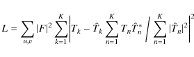
The assumption of additive Gaussian noise leads to a maximum-likelihood estimate of the object and transfer functions, equivalent to the solution of a conventional non-linear least-squares fit problem, and corresponds to the minimization of the scalar quantity L,
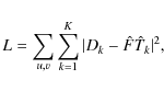
where u,v represents pixels in Fourier space. This equation directly leads to an optimum estimate
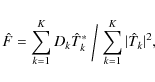
(Paxman et al. 1992), where
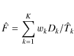
where
and
3 Compensation for uncorrected high-order aberrations
MFBD and related image reconstruction techniques do not rely on statistical properties of seeing, thereby allowing compensation for individual telescope aberrations and the effects of an adaptive optics (AO) system in addition to seeing-induced aberrations. By estimating the transfer function for each recorded frame, a small number of exposures can be used to restore the object. However, the number of aberration coefficients that can be determined from focused and defocused images is necessarily limited. In less than perfect seeing, this leaves a partially compensated PSF with enhanced wings. This corresponds to the well-known ``halo'' seen in images of point-like objects recorded with night-time telescopes and partial AO compensation of seeing (e.g., Conan et al. 1992).
3.1 Seeing statistics and residual aberrations expected
To appreciate the importance of residual high-order aberrations, we note that Danilovic et al. (2008) found that aberrations as small as 0.044 waves, corresponding to nearly perfect optics with a Strehl ratio of 93%, reduces the measured rms contrast of granulation from 8.4% to 8.1% with Hinode's spectro-polarimeter. Thus, within the framework of the present investigation, we clearly should consider any residual aberrations that decrease the Strehl ratio below 90%.
The effect of partially corrected aberrations on the Strehl ratio is
well-known from the work of Fried, Noll, Wang, Markey and others. We
refer to Roddier (1999) for an overview of relevant
results. The residual wavefront variance for zonal correction can be
estimated as
where
The Strehl ratio R can be estimated as

We shall in the following estimates assume perfect zonal correction, which in the case of AO correction would represent an unrealistically high efficiency. For the SST, with a telescope diameter of 0.98 m, we find that R=0.81 with N=36 aberration parameters when r0=22 cm and that R>0.9 only when r0>33 cm. With good seeing corresponding to r0=10 cm (1
An important limitation at short wavelengths is that r0 scales as
![]() .
When r0=20 cm at
.
When r0=20 cm at
![]() nm, r0 is
only 11 cm at 390 nm. In this case we need to compensate nearly 100
aberrations at 630 nm and over 300 aberrations at 390 nm to reach a
Strehl ratio of 0.9. Even in excellent seeing, images recorded and
processed with conventional MFBD at 390 nm will be far from perfectly
corrected. It is therefore not surprising that measured rms contrasts
of granulation with the SST show much larger discrepancies with 3D
simulations at short wavelengths than at long wavelengths.
nm, r0 is
only 11 cm at 390 nm. In this case we need to compensate nearly 100
aberrations at 630 nm and over 300 aberrations at 390 nm to reach a
Strehl ratio of 0.9. Even in excellent seeing, images recorded and
processed with conventional MFBD at 390 nm will be far from perfectly
corrected. It is therefore not surprising that measured rms contrasts
of granulation with the SST show much larger discrepancies with 3D
simulations at short wavelengths than at long wavelengths.
3.2 Compensation for high-order aberrations
In MOMFBD processing of SST data, particularly from the CRISP
instrument (Scharmer et al. 2008), a data set corresponding to a line
scan can consist of ![]() 1000 exposures in several cameras. However,
an estimated object from a particular wavelength and polarization
state is typically based on deconvolution of a relatively small
number of images (
1000 exposures in several cameras. However,
an estimated object from a particular wavelength and polarization
state is typically based on deconvolution of a relatively small
number of images (![]() 10), degraded by residual low-order
aberrations from partial correction with a 37-electrode AO system and
uncorrected high-order atmospheric aberrations. As long as MFBD
processing compensates the residual aberrations partially corrected by
the AO system, we are to some extent justified in ignoring the
corrections made by the AO system: It is the residual aberrations
after that AO correction that define the S/N of individual
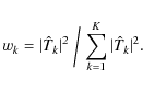
images and the weighting implied by Eq. (4).
10), degraded by residual low-order
aberrations from partial correction with a 37-electrode AO system and
uncorrected high-order atmospheric aberrations. As long as MFBD
processing compensates the residual aberrations partially corrected by
the AO system, we are to some extent justified in ignoring the
corrections made by the AO system: It is the residual aberrations
after that AO correction that define the S/N of individual
images and the weighting implied by Eq. (4).
Our goal is to estimate the effect on the transfer function of uncompensated high-order aberrations, defined in Eq. (11). To do this, we will assume that these modes have amplitudes given by the assumption of Kolmogorov turbulence. This is the same basic assumption as used in Speckle Interferometry, but with the difference that low-order modes are compensated individually and for each exposed frame with MFBD. We conjecture that:
- there will be rather small variations of the PSF from one frame to another because residual wavefront errors, after correction on the order of 30 modes, depend on the accumulative effect of hundreds of modes rather than a few large-amplitude low-order modes;
- a relatively small number of frames is therefore needed to obtain stable averages.
3.2.1 The proposed method
Our goal is to develop a method that combines the advantages of MFBD/JPDS and speckle methods. The approach taken is to compensate individual frames for low-order modes and to add a compensation for the average effect of hundreds of high-order aberrations from atmospheric turbulent seeing.
This compensation can be implemented in various ways. We have chosen
the following simple approach that has the advantage of not involving
the observed images but only their corresponding transfer functions.
We note that information about the ``true'' (exact) transfer functions
and the true object are encoded in the observed images. Ignoring the
noise term in Eq. (1) and combining with
Eq. (3), we obtain a relation between the estimated object
![]() ,
the true object F, and the corresponding exact and
estimated transfer functions Tk and
,
the true object F, and the corresponding exact and
estimated transfer functions Tk and
![]()
We note that this is a relation of the form

i.e., in the form of a multiplication of the true object with a transfer function,
that is a weighted average of the ratio of the true and estimated transfer equations. This equation does not solve the problem unless the exact transfer functions are known. However, we can estimate S by including known statistical properties of atmospheric high-order aberrations while using MFBD or JPDS estimates of low-order aberrations for each individual exposure. We propose the following estimate of S from a combination of aberration parameters determined by MFBD/JPDS processing and statistical properties of atmospheric seeing:

where angular brackets,
To estimate the effect of high-order aberrations in Tk, we add random higher-order KL modes with amplitudes given by Kolmogorov statistics and average the transfer equation over many realizations to obtain stable averages. The proposed method requires measurements of r0 at the time of recording the data. The preferable method for accurate measurements of r0 is via data from an open-loop wavefront sensor located before the adaptive mirror, as implemented at the SST (Scharmer & van Werkhoven 2010). It is also possible, as done at the Dunn telescope diameter (Marino et al. 2004), to combine closed-loop wavefront sensor data with the control matrix and output voltages to estimate r0 and residual low-order aberrations. The quality of such measurements are to some extent limited by time delays and inaccuracies in the control matrix, but experience with night-time AO systems clearly indicates that good PSF compensation is indeed possible with such data (Veran et al. 1997).
4 Simulations
To investigate the feasibility of the proposed method for compensation of missing high-order aberrations in MFBD and JPDS processing, numerical calculations and simulations were made.
4.1 Ideal compensation with point sources
![\begin{figure}
\par\includegraphics[bb=46 632 556 787,width=18cm]{14800fg1}
\end{figure}](/articles/aa/full_html/2010/13/aa14800-10/img40.png)
|
Figure 1:
PSFs displayed in log scale. The circles mark 90%
encircled energy, see also Fig. 2. Far
left: Diffraction limited. Top: PSFs corresponding to
S, i.e., true residual high-order aberrations for different
r0 as indicated.
Bottom: Approximate PSFs, corresponding to |
| Open with DEXTER | |
| Figure 2:
Encircled PSF energy for different r0 as indicated in
the figure. Red: PSFs based on S; Blue: PSFs based on |
|
| Open with DEXTER | |
| Figure 3:
Strehl ratios as a function of r0. Solid line:
Eqs. (7) and (8) with N=37; Red plus
(+) symbols: PSFs based on S; Blue cross ( |
|
| Open with DEXTER | |
| Figure 4:
Power spectra (angular averages) of S (red) and |
|
| Open with DEXTER | |
![\begin{figure}
\par\includegraphics[bb=46 620 556 787,width=18cm]{14800fg5}
\end{figure}](/articles/aa/full_html/2010/13/aa14800-10/img44.png)
|
Figure 5:
Synthetic images calculated at a wavelength of 630 nm.
Far left: Original image. Top: Low-pass images
degraded by high-order aberrations, i.e., by S, corresponding to
r0=25, 20, 15, 10, 7 and 5 cm, resp. (same layout as
Fig. 1).
Bottom: Degraded images compensated by use of the method
described, i.e., by |
| Open with DEXTER | |
We used KL functions based directly on the theory of Fried (1978), as implemented by Dai (1995). These functions are orthogonal on a circular aperture and statistically independent for Kolmogorov turbulence. For such turbulence, the variances depend only on r0. To produce random wavefronts following Kolmogorov statistics, 1001 random numbers were drawn from a standard normal distribution, scaled with the square root of the theoretical variances and used as coefficients for KL functions 4-1004 (in decreasing variance order). The resulting wavefronts were scaled to different values of Fried's parameter r0. To simulate the effect of partial correction with an efficient AO system, we reduced the amplitudes of KL coefficients 4-37 with a factor 4 (this represents an overestimate of the actual efficiency). Piston (coefficient 1) is ignored because it does not contribute to the OTFs and tip-tilt correction (coefficients 2 and 3) was assumed to be perfect, corresponding to images recorded with sufficiently short exposure times to remove changes in image position and blurring during the exposure.
The residuals of the AO-corrected aberrations were used to represent
the estimate of the transfer equations ![]() .
For this
calculation we assumed 10 observed images with independently obtained
wavefronts. We computed the ``corrective'' transfer function S from
Eq. (11) by using the actual high-order aberrations
corresponding to each Tk and then the approximate version,
.
For this
calculation we assumed 10 observed images with independently obtained
wavefronts. We computed the ``corrective'' transfer function S from
Eq. (11) by using the actual high-order aberrations
corresponding to each Tk and then the approximate version, ![]() ,
using the statistical averages (based on 100 realizations of the
high-order tail) of the transfer functions, as defined in
Eq. (12). We finally compared the exact and estimated
transfer functions S and
,
using the statistical averages (based on 100 realizations of the
high-order tail) of the transfer functions, as defined in
Eq. (12). We finally compared the exact and estimated
transfer functions S and ![]() .
This corresponds to perfect MFBD
correction of the first 36 KL modes and perfect knowledge of r0.
.
This corresponds to perfect MFBD
correction of the first 36 KL modes and perfect knowledge of r0.
Figure 1 shows the PSFs corresponding to S and ![]() ,
scaled such that the wings of the PSFs can be seen, for values of
r0 in the range 5-25 cm and
,
scaled such that the wings of the PSFs can be seen, for values of
r0 in the range 5-25 cm and
![]() nm. Calculations were
made for a 98 cm telescope diameter, corresponding to the SST, with
critical sampling at
nm. Calculations were
made for a 98 cm telescope diameter, corresponding to the SST, with
critical sampling at
![]() nm, corresponding to
nm, corresponding to
![]() .
The field of view (FOV) shown is
.
The field of view (FOV) shown is
![]() .
As expected, the true PSFs show a speckled
structure in the wings, but smoothed by the averaging effect obtained
by combining ten images. The corresponding approximate PSFs show much
less structure in the wings but are otherwise similar to the actual
PSFs. It can also be seen that the effective diameter of the PSF,
defined as that containing 90% of the energy of the PSF, increases
with decreasing r0. When r0 equals 25 cm, that diameter is
approximately 1
.
As expected, the true PSFs show a speckled
structure in the wings, but smoothed by the averaging effect obtained
by combining ten images. The corresponding approximate PSFs show much
less structure in the wings but are otherwise similar to the actual
PSFs. It can also be seen that the effective diameter of the PSF,
defined as that containing 90% of the energy of the PSF, increases
with decreasing r0. When r0 equals 25 cm, that diameter is
approximately 1
![]() 1, when r0 is 5 cm, it increases to
approximately 4
1, when r0 is 5 cm, it increases to
approximately 4
![]()
![]() .
Figure 2 shows the encircled energy as function of
radius for the approximate and exact PSFs. It is clear that the
encircled energy of the approximate PSF follows that of the actual PSF
nearly exactly. In Fig. 3 we show calculated Strehl
ratios of the PSFs as function of r0. The exact and approximate
PSFs give nearly exactly the same Strehl ratios and also agree well
with what is expected for perfect KL correction of 36 modes from
Eqs. (7) and (8). Finally,
Fig. 4 shows radially averaged power spectra for the
transfer functions corresponding to the exact and approximate PSFs,
again showing an excellent agreement between the two at all spatial frequencies.
We also refer the reader to Fig. 12 by Rouppe van der Voort et al. (2004), where similar effects of seeing on observed power spectra of penumbral fine structure are discussed.
.
Figure 2 shows the encircled energy as function of
radius for the approximate and exact PSFs. It is clear that the
encircled energy of the approximate PSF follows that of the actual PSF
nearly exactly. In Fig. 3 we show calculated Strehl
ratios of the PSFs as function of r0. The exact and approximate
PSFs give nearly exactly the same Strehl ratios and also agree well
with what is expected for perfect KL correction of 36 modes from
Eqs. (7) and (8). Finally,
Fig. 4 shows radially averaged power spectra for the
transfer functions corresponding to the exact and approximate PSFs,
again showing an excellent agreement between the two at all spatial frequencies.
We also refer the reader to Fig. 12 by Rouppe van der Voort et al. (2004), where similar effects of seeing on observed power spectra of penumbral fine structure are discussed.
4.2 Ideal compensation with granulation images
To investigate the effects of uncompensated high-order aberrations on
granulation images, we used synthetic images calculated from a field-free 3D MHD
simulation (Stein & Nordlund 1998); these simulation data were
kindly provided by Mats Carlsson. The synthetic images were calculated
at a wavelength of 630 nm and were degraded to a resolution
corresponding to 90% of the diffraction limit of the SST while
keeping the image scale of the original synthetic images. The images
were then degraded by Fourier multiplication with S based on 10
wavefronts. This corresponds to an MFBD estimate ![]() based on 10
observed images.
based on 10
observed images. ![]() was then corrected using an approximate
was then corrected using an approximate
![]() based on the same low-order aberrations as S and a
high-order compensation with 1000 KL-modes according to
Eq. (12). The original, degraded and restored images are
shown in Fig. 5 together with their rms contrasts.
Note that the degraded images differ from the original image in
contrast but not in fine structure shown. The main effect of the
higher-order aberrations is to add stray light, decreasing the rms
contrast, whereas all small-scale features of the original image are
retained and restored to full contrast with the approximate PSFs. As
shown in Fig. 5, the loss in contrast is from 14.5%
to 11.8% when r0 is 15 cm, or a reduction of the rms contrast by
nearly 20%. This corresponds to very good seeing conditions. In more typical seeing conditions, when r0 is 10 cm or smaller, the effects are larger.
based on the same low-order aberrations as S and a
high-order compensation with 1000 KL-modes according to
Eq. (12). The original, degraded and restored images are
shown in Fig. 5 together with their rms contrasts.
Note that the degraded images differ from the original image in
contrast but not in fine structure shown. The main effect of the
higher-order aberrations is to add stray light, decreasing the rms
contrast, whereas all small-scale features of the original image are
retained and restored to full contrast with the approximate PSFs. As
shown in Fig. 5, the loss in contrast is from 14.5%
to 11.8% when r0 is 15 cm, or a reduction of the rms contrast by
nearly 20%. This corresponds to very good seeing conditions. In more typical seeing conditions, when r0 is 10 cm or smaller, the effects are larger.
We conclude that whereas details of the exact and approximate PSFs certainly differ, the overall effect of the high-order aberrations is to add spatial stray light to the images. The proposed method for statistical compensation of high-order aberrations in principle should work very well.
![\begin{figure}
\par\mbox{\subfigure[]{\includegraphics[bb=34 24 196 283,clip,wid...
...]{\includegraphics[bb=34 24 196 283,clip,width=3cm]{14800fg6l} }}
\end{figure}](/articles/aa/full_html/2010/13/aa14800-10/img46.png)
|
Figure 6:
RMS intensity error (in % of the average intensity) of
restored granulation images as a function of r0 (in cm) after
correcting M modes. Circles ( |
| Open with DEXTER | |
4.3 Inversion tests with granulation images
With perfect determination of the low-order modes, correction of the high order modes in a statistical sense gives excellent results. However, we also need to investigate the effect of realistic errors from the low-order modes estimated with MFBD and JPDS techniques.
For this test, we calculated 1000 random wavefronts corresponding to
Kolmogorov statistics, with reduced amplitudes for the first 36 KL
coefficients as described above. These wavefronts, scaled to different
r0, were used to construct sets of degraded granulation images
with and without phase diversity, corresponding to an added focus
shift, of 1 wave peak-to-valley. We used synthetic images calculated
from the 3D MHD code as true objects,
compressed by a factor 2 (by cropping the Fourier transform of the
image). The image scale was set to match that of SST/CRISP during the
2009 observing season,
![]() ,
corresponding to
about 12% oversampling at 630 nm.
,
corresponding to
about 12% oversampling at 630 nm.
The degraded synthetic images were processed with the MOMFBD program
in various ways (MFBD or JPDS, different numbers of realizations,
different subfield sizes (256 pixels = 15
![]() ,
128 pixels =
7
,
128 pixels =
7
![]() 6, 80 pixels = 4
6, 80 pixels = 4
![]() 7), different number of estimated
wavefront parameters, with and without added noise).
7), different number of estimated
wavefront parameters, with and without added noise).
![\begin{figure}
\par\mbox{\subfigure[]{\includegraphics[bb=38 24 196 283,clip,wid...
...]{\includegraphics[bb=38 24 196 283,clip,width=3cm]{14800fg7e} }}
\end{figure}](/articles/aa/full_html/2010/13/aa14800-10/img48.png)
|
Figure 7: Wavefront quantities as a function of M (number of corrected modes) for r0=10 cm. Red: rms wavefront in rad; Blue: rms wavefront residual in rad. |
| Open with DEXTER | |
![\begin{figure}
\par\mbox{\subfigure[]{\includegraphics[bb=38 24 196 283,clip,wid...
...hics[bb=38 24 196 283,clip,width=3cm]{14800fg8e} }}
\vspace*{-2mm}
\end{figure}](/articles/aa/full_html/2010/13/aa14800-10/img49.png)
|
Figure 8: Strehl ratio as a function of M (number of corrected modes) for r0=10 cm. |
| Open with DEXTER | |
4.3.1 Results without
 compensation
Figure 6 shows rms intensity errors of restored images
using different techniques (MFBD, JPDS), number of aberration
parameters (M=35, 50 and 100) with and without ![]() compensation
for different values of Fried's parameter r0. We emphasize that for
all calculations made, 1000 frames were used to obtain the wavefronts
but in panels d-f and j-l subsets of only 10 frames were used to
restore the images. This corresponds to processing of SST/CRISP data,
where the broad-band channel of a MFBD or JPDS data set corresponds to
on the order of 500-1000 images. The simultaneously exposed
narrow-band CRISP images are divided into typically 10-12 wavelength
bins, each with 4 polarization bins. These narrow-band images are
restored individually, but using the aberrations (mainly) determined
by the 1000 broadband images. The upper row of plots show the results
obtained without noise and the bottom row show the corresponding
results with 0.5% Gaussian noise added to the simulated images.
compensation
for different values of Fried's parameter r0. We emphasize that for
all calculations made, 1000 frames were used to obtain the wavefronts
but in panels d-f and j-l subsets of only 10 frames were used to
restore the images. This corresponds to processing of SST/CRISP data,
where the broad-band channel of a MFBD or JPDS data set corresponds to
on the order of 500-1000 images. The simultaneously exposed
narrow-band CRISP images are divided into typically 10-12 wavelength
bins, each with 4 polarization bins. These narrow-band images are
restored individually, but using the aberrations (mainly) determined
by the 1000 broadband images. The upper row of plots show the results
obtained without noise and the bottom row show the corresponding
results with 0.5% Gaussian noise added to the simulated images.
Discussing first the results without ![]() compensation (blue
symbols), our reference for comparison is the results obtained using
1000 frames to restore the image and the first M true (exact)
aberration parameters (panel a). This shows the expected behavior: The
quality of the restored images improves with increasing value of r0and also with increasing number of estimated aberration parameters
used to restore the images. When r0 is 20 cm, the rms error with 50
perfectly known aberration parameters is only 1.5%. However, in more
typical seeing conditions (r0=10 cm or smaller), the corresponding
rms error is 2.5-8%, depending on the number of aberration
parameters compensated and the seeing quality.
compensation (blue
symbols), our reference for comparison is the results obtained using
1000 frames to restore the image and the first M true (exact)
aberration parameters (panel a). This shows the expected behavior: The
quality of the restored images improves with increasing value of r0and also with increasing number of estimated aberration parameters
used to restore the images. When r0 is 20 cm, the rms error with 50
perfectly known aberration parameters is only 1.5%. However, in more
typical seeing conditions (r0=10 cm or smaller), the corresponding
rms error is 2.5-8%, depending on the number of aberration
parameters compensated and the seeing quality.
Figure 6b (MFBD processing with 1000 frames) demonstrates that the rms intensity error obtained using only focused images to estimate the aberration parameters shows quite small variation of the intensity error with the number of aberration parameters M, when M is in the range 35-100. The rms intensity error for M=35 MFBD calculations actually corresponds to what was obtained with the true aberration parameters for M=100 (Panel a)! This implies that MFBD processing with a given number of aberration parameters leads to estimates of the transfer function that compensate for the effects of missing higher-order aberration parameters (truncation of the wavefront). Increasing the number of estimated aberration parameters from 35 to 50 or 100, reduces the efficiency of this compensation such that the reduction of the intensity error is relatively modest. Quite clearly, the estimated wavefront with MFBD processing must be inaccurate, but such that the estimated transfer function accurately represents the true transfer function. This conclusion is further supported by Fig. 7, which shows the variation of the (estimated) wavefront rms and wavefront error for different number of estimated wavefront parameters when r0=10 cm. Panel a (red symbols) shows that the rms of the true wavefront increases by 50% when M is increased from 35 to 100. In contrast, the rms of the estimated wavefront for the M first aberration parameters is strongly overestimated for M=35and M=50 with MFBD processing such that the estimated wavefront rms is nearly independent of M. Thus, using a low-order or high-order representation for the wavefront leads to nearly the same estimated wavefront rms. A striking result is that MFBD processing of the first 35-100 corrected modes leads to residual wavefront errors (blue symbols) that are larger than if the wavefront is estimated to be exactly zero!
When using also a defocused channel (JPDS processing), the wavefronts are more constrained to represent reality, leading to smaller wavefront errors (Fig. 7c). But this constraint also limits the freedom in compensating the transfer function for high-order aberrations, such that larger intensity errors are obtained in the restored images with JPDS (Fig. 6c) than with MFBD processing (Fig. 6b).
These conclusions about differences between MFBD and JPDS processing
are supported by the Strehl ratios calculated from wavefronts
determined with the granulation images and shown in
Fig. 8. With true aberration parameters
(Fig. 8a) and without ![]() compensation,
the Strehl intensity increases gradually with the number of
compensated aberration parameters M. However, with MFBD processing,
the Strehl ratio is constant when M is in the range 35-100. The
Strehl ratio achieved, R=0.8, is close to what is expected from
Eqs. (6) and (8) for N=M=100. The variation of
the Strehl ratio with M obtained with JPDS processing is
intermediate to that of MFBD and using the true aberration parameters.
compensation,
the Strehl intensity increases gradually with the number of
compensated aberration parameters M. However, with MFBD processing,
the Strehl ratio is constant when M is in the range 35-100. The
Strehl ratio achieved, R=0.8, is close to what is expected from
Eqs. (6) and (8) for N=M=100. The variation of
the Strehl ratio with M obtained with JPDS processing is
intermediate to that of MFBD and using the true aberration parameters.
Adding 0.5% Gaussian noise to the MFBD data shows that the results are sensitive to noise (Figs. 6h-i) and indicates that in practice the compensation effects discussed above will not be large and that the quality of MFBD and JPDS image restorations should be rather similar. The rms intensity error improvement is limited to that corresponding to about 50 ``true'' aberration parameters, or a Strehl ratio of 0.7. Using more than 50 aberration parameters to represent the wavefront does not significantly improve the quality of the restored images.
4.3.2 Results with
compensation
![\begin{figure}
\par\mbox{ \subfigure[]{\includegraphics[angle=0,width=4.5cm]{148...
... \subfigure[]{\includegraphics[angle=0,width=4.5cm]{14800fg9d} }}
\end{figure}](/articles/aa/full_html/2010/13/aa14800-10/img51.png)
|
Figure 9: Sample wavefronts from the simulation experiments. a)-d): Different realizations of the Kolmogorov statistics. Within each sub-figure, all wavefronts are displayed with identical scaling. Left: True wavefronts; Center: JPDS estimated wavefronts; Right: MFBD estimated wavefronts. 1st row: 35 KL modes; 2nd row: 50 modes; 3rd row: 100 modes; 4th row: All 1001 modes. |
| Open with DEXTER | |
The results obtained with ![]() compensation are shown with red
symbols in Fig. 6. With such compensation,
restorations with ``true'' low-order wavefronts allow nearly
perfectly restored images, even with 10 frames, in bad seeing
(r0=7 cm) and using only 35 aberration parameters. This
re-enforces our earlier conclusion, that details of the high-order
part of the wavefront are not important as long as it has the
``right'' statistical properties. In particular, the ``speckles'' seen
in the wings of the PSF of Fig. 1 (upper row), have a
small effect on the restored images. The excellent result obtained
with
compensation are shown with red
symbols in Fig. 6. With such compensation,
restorations with ``true'' low-order wavefronts allow nearly
perfectly restored images, even with 10 frames, in bad seeing
(r0=7 cm) and using only 35 aberration parameters. This
re-enforces our earlier conclusion, that details of the high-order
part of the wavefront are not important as long as it has the
``right'' statistical properties. In particular, the ``speckles'' seen
in the wings of the PSF of Fig. 1 (upper row), have a
small effect on the restored images. The excellent result obtained
with ![]() compensation based on ``true'' wavefronts also is
consistent with the results discussed previously: that MFBD processing
with 35 aberration parameters can produce transfer functions
equivalent to those obtained with compensation by 100 aberration
parameters, even though the actual wavefronts derived are
demonstratedly wrong.
compensation based on ``true'' wavefronts also is
consistent with the results discussed previously: that MFBD processing
with 35 aberration parameters can produce transfer functions
equivalent to those obtained with compensation by 100 aberration
parameters, even though the actual wavefronts derived are
demonstratedly wrong.
With MFBD processing, the improvement from ![]() compensation
varies strongly with the number of aberration parameters, M. The
remarkably good results obtained without
compensation
varies strongly with the number of aberration parameters, M. The
remarkably good results obtained without ![]() compensation for
M=35 and M=50 constitutes a problem with
compensation for
M=35 and M=50 constitutes a problem with ![]() compensation! This is because our calculations of
compensation! This is because our calculations of ![]() do not take
into account the compensation for high-order aberrations already
provided by the MFBD (and JPDS) processing. This leads to an
overcompensation of the effects of high-order aberrations for
M=35 and M=50. This compensation is much smaller with M=100.
With JPDS processing (panels c, f, i and l), the results show improved
consistency. Here,
do not take
into account the compensation for high-order aberrations already
provided by the MFBD (and JPDS) processing. This leads to an
overcompensation of the effects of high-order aberrations for
M=35 and M=50. This compensation is much smaller with M=100.
With JPDS processing (panels c, f, i and l), the results show improved
consistency. Here, ![]() compensation with M=50 or M=100 leads
to rms intensity errors that are reduced by a factor 2-3. The
obtained rms errors are consistently smaller than for MFBD processing
without
compensation with M=50 or M=100 leads
to rms intensity errors that are reduced by a factor 2-3. The
obtained rms errors are consistently smaller than for MFBD processing
without ![]() compensation, when noise is present.
compensation, when noise is present.
We have here demonstrated that MFBD image reconstruction by itself
allows compensation effects by fitting transfer functions rather than
wavefronts. In this sense, MFBD or JPDS processing provides more
optimum image reconstruction than with a Shack-Hartmann based
wavefront sensor. The main problem in the present context is that MFBD
and (to a smaller extent) JPDS processing already introduces part of
the compensation intended to be performed with ![]() .
This leads to
overcompensation if no counter measures are taken. By using JPDS
processing, the compensation effects are constrained and the risk of
overcompensation with
.
This leads to
overcompensation if no counter measures are taken. By using JPDS
processing, the compensation effects are constrained and the risk of
overcompensation with ![]() is small.
is small.
The relatively poor estimates of the wavefronts obtained with MFBD and JPDS processing may appear to contradict earlier simulations with phase diversity methods (Löfdahl & Scharmer 1994; Paxman et al. 1996), but are a direct consequence of the assumed AO correction, reducing the rms amplitudes of the first 35 KL aberrations with a factor of 4. This leaves residual wavefronts that have small or negligible amplitudes for the first 35 modes and a correspondingly large contribution from higher-order modes. This leads to significant cross-talk from high-order aberrations, degrading the low-order wavefront estimates but actually leading to better estimates of the transfer functions than expected on the basis of the number of aberration parameters included. Figure 9 shows the wavefronts corresponding to the first 4 frames used to reconstruct the image with 10 frames. In the left column are shown (top to bottom) the true wavefronts represented with 35, 50, 100 and 1001 KL modes. It is evident from the lower-left wavefront in each panel that the true wavefront has been stripped of its low-frequency wavefront components. It is also evident that the JPDS (mid column) and MFBD (right column) wavefront estimates show large differences and that JPDS provides the best estimate of the true wavefront.
4.4 Inversion tests with point sources
We have also made inversion tests with point sources. While not
directly relevant for restoration of solar images, these tests do shed
further light on the MFBD and JPDS compensation effects discussed
above. The most striking result is that both MFBD and JPDS processing
of synthetic noise-free point source images lead to nearly perfectly
reproduced low-order wavefronts.
To understand why granulation images and images of point sources lead
to different wavefront estimates, we express the equation used to
estimate the transfer function as follows: inserting the expression
for ![]() in Eq. (3) into Eq. (2), and
replacing Dk with F Tk, we obtain an expression for the error
metric L that corresponds to the scalar quantity minimized in MFBD
and JPDS processing:
in Eq. (3) into Eq. (2), and
replacing Dk with F Tk, we obtain an expression for the error
metric L that corresponds to the scalar quantity minimized in MFBD
and JPDS processing:
|
(13) |
Ignoring the complicated expression involving the exact and estimated transfer functions Tk and
4.5 Comment on the use of small subfields
The results discussed above were all obtained with
![]() -pixel subfields. Calculations with
-pixel subfields. Calculations with
![]() -pixel
subfields gave results that are virtually identical to those
discussed. MFBD calculations with
-pixel
subfields gave results that are virtually identical to those
discussed. MFBD calculations with
![]() -pixel subfields gave
poorer, but still acceptable, results. However, JPDS restorations with
-pixel subfields gave
poorer, but still acceptable, results. However, JPDS restorations with
![]() -pixel subfields essentially failed. This is attributed to
the relatively large diameter of the PSF corresponding to the
defocused images, causing problems from lack of information
about the object outside the subfield and wrap-around effects when
using FFTs to perform convolutions with the defocused PSF. It is thus
more difficult to use small subfields with JPDS than with MFBD with
the present methods.
-pixel subfields essentially failed. This is attributed to
the relatively large diameter of the PSF corresponding to the
defocused images, causing problems from lack of information
about the object outside the subfield and wrap-around effects when
using FFTs to perform convolutions with the defocused PSF. It is thus
more difficult to use small subfields with JPDS than with MFBD with
the present methods.
5 Tests with real data
5.1 Observations
To test the proposed ![]() compensation method we used granulation
images recorded through a 0.44 nm FWHM 2-cavity filter centered at
630.26 nm and a 0.34 nm filter centered at 538.20 nm, both used as
wide-band channels for the SST/CRISP imaging spectro-polarimeter
(Scharmer et al. 2008).
The images were exposed by means of a
rotating chopper, set to give exposure times of 16 ms and a dark
read-out time of nearly 12 ms, corresponding to an overall frame rate
of 36 Hz. The 630 nm and 538 nm data discussed here were
recorded between 10:45 and 10:50 UT on 26 June 2009, during a period
with reasonably good but strongly variable seeing. The science target
for these observations was a small
pore in AR 1023, located at approximately S22, W20, corresponding to a
heliocentric distance of about
compensation method we used granulation
images recorded through a 0.44 nm FWHM 2-cavity filter centered at
630.26 nm and a 0.34 nm filter centered at 538.20 nm, both used as
wide-band channels for the SST/CRISP imaging spectro-polarimeter
(Scharmer et al. 2008).
The images were exposed by means of a
rotating chopper, set to give exposure times of 16 ms and a dark
read-out time of nearly 12 ms, corresponding to an overall frame rate
of 36 Hz. The 630 nm and 538 nm data discussed here were
recorded between 10:45 and 10:50 UT on 26 June 2009, during a period
with reasonably good but strongly variable seeing. The science target
for these observations was a small
pore in AR 1023, located at approximately S22, W20, corresponding to a
heliocentric distance of about
![]() (
(
![]() ).
This pore was also used as lock point for the AO system. However, in
the present paper we discuss only field-free granulation outside this
active region. The noise level in the recorded images was estimated
from power spectra at high spatial frequencies and found to
be about 0.9%.
).
This pore was also used as lock point for the AO system. However, in
the present paper we discuss only field-free granulation outside this
active region. The noise level in the recorded images was estimated
from power spectra at high spatial frequencies and found to
be about 0.9%.
CRISP was used to repeatedly scan each of the 630.26 nm
and 538.20 nm
lines three times, using different numbers of wavelength positions for
the two lines. These scans required a total of 17 s for the
630 nm line and 12 s for the 538 nm line, setting the
time between pre-filter changes. Simultaneously, approximately 600
wide-band
images were collected at 630 nm and ![]() 433
images at 538 nm during
each scan. We refer to these 17 s and 12 s sets of wide-band
images as ``full scan'' data sets but will primarily discuss the
results of processing 2.2 s sub-sets of this data to match the
time-scale of seeing changes.
433
images at 538 nm during
each scan. We refer to these 17 s and 12 s sets of wide-band
images as ``full scan'' data sets but will primarily discuss the
results of processing 2.2 s sub-sets of this data to match the
time-scale of seeing changes.
The images were corrected for gain and bias and MFBD processed with the MOMFBD code, see Sect. 5.3 below.
5.2 Seeing measurements
Simultaneous measurements of Fried's parameter r0 were obtained
with the SST wide-field wavefront sensor (WFWFS;
Scharmer & van Werkhoven 2010), developed as part of an effort to characterize
day-time high-altitude seeing at La Palma. The WFWFS is mounted on a
beam that splits off light immediately before the tip-tilt and
deformable mirrors, such that r0 can be measured through the
telescope and from a FOV that is adjacent to the science FOV, but
without impact from the AO system. Between UT 10:00 and 10:48,
processed WFWFS data averaged over 100 s gave estimates of r0 in
the range 11-12 cm at 500 nm, corresponding to 15-16 cm at 630 nm
and 12-13 cm at 538 nm. However, the science images, recorded with
the AO system in closed loop, showed strong variations in image
quality on time scales on the order of a few seconds. The WFWFS variances measured are proportional to
r0-5/3 (Eqs. (7)-(8); Scharmer & van Werkhoven 2010), such that averaging wavefront sensor data in variable seeing gives the largest weights to relatively poor seeing (small
values of r0). However, MFBD image restoration gives the highest
weights to good images (large values of r0). We therefore
compare data recorded over such short time intervals that
r0 can be considered constant. We re-processed the WFWFS data in
blocks of 2.2 s, or about 10 WFWFS CCD frames. Figure
10 shows in the upper panel the variation of
r0 with time from UT 10:45-10:50, obtained from overlapping 2.2-s
blocks of WFWFS data. The red and blue curves in this panel indicate
the wavelengths at which the science images were recorded, at 630 nm
and 538 nm respectively. In the mid panel is shown the variation of
the rms contrast measured (see Sect. 5.4.1) for the 630 nm and 538 nm images
after flat-fielding but without MOMFBD image restoration. Comparing
the two panels, there is a clear correlation between r0 and the
measured rms contrast; even small and rapid variations are reproduced
in detail. The bottom panel shows the correlation between all measured
values of r0 and the rms contrast. In this figure, we have scaled
the r0 values measured with the WFWFS at 500 nm to 538 nm and
630 nm by assuming that r0 is proportional to
![]() .
We
have also multiplied all rms contrasts at 630 nm by an ad hoc factor
1.22, roughly compensating for the wavelength dependence of the
granulation contrast. The plotted values cover a range of r0 from
4 cm to nearly 30 cm and rms contrast from 2.2% to 7.8% and show an
excellent correlation. The dotted curve corresponds to variation of
the rms contrast with r0 obtained from the simulations shown in
Fig. 5, but divided by a factor 1.85 to fit the data. This large
factor in part comes from the assumed perfect compensation of the
first 35 KL modes, corresponding to an AO system with 100%
efficiency, and in part must be due to stray light.
.
We
have also multiplied all rms contrasts at 630 nm by an ad hoc factor
1.22, roughly compensating for the wavelength dependence of the
granulation contrast. The plotted values cover a range of r0 from
4 cm to nearly 30 cm and rms contrast from 2.2% to 7.8% and show an
excellent correlation. The dotted curve corresponds to variation of
the rms contrast with r0 obtained from the simulations shown in
Fig. 5, but divided by a factor 1.85 to fit the data. This large
factor in part comes from the assumed perfect compensation of the
first 35 KL modes, corresponding to an AO system with 100%
efficiency, and in part must be due to stray light.
![\begin{figure}
\par\includegraphics[bb=10 10 493 343,clip,width=9cm]{14800fg10a}...
...0b}
\includegraphics[bb=10 9 493 343,clip,width=9cm]{14800fg10c}
\end{figure}](/articles/aa/full_html/2010/13/aa14800-10/img58.png)
|
Figure 10:
Variation of Fried's parameter r0 with time, measured
with the SST wide-field wavefront sensor bypassing the AO system
( top panel) and the corresponding variation of the measured
granulation rms contrast of the science images ( mid panel)
obtained at
|
| Open with DEXTER | |
Our conclusion from the excellent correlation between measured variations of r0 with the WFWFS (bypassing the AO system) and the science images (recorded with the AO system in closed loop) is that the WFWFS indeed provides an accurate measure of seeing, although we cannot from this data rule out systematic errors, such as a scale factor error or a systematic bias, in the measured r0 values.
5.3 MFBD processing
The MOMFBD software package was used to divide the images into
![]() -pixel overlapping subfields, which were separately MFBD
restored using the M=100 most significant KL modes. The restored
subfields were then mosaicked to produce restored images over the
entire observed FOV. To investigate the effects of strongly variable
seeing on the MFBD processing, we processed the data in blocks
corresponding to about 2.2 s of data as well as in blocks
corresponding to full scans (12 s resp. 17 s data). To allow a
comparison between the two methods of processing, subsets of the full
scan MFBD wavefronts and observed images were used to restore the same raw images as used with the 2.2 s data.
-pixel overlapping subfields, which were separately MFBD
restored using the M=100 most significant KL modes. The restored
subfields were then mosaicked to produce restored images over the
entire observed FOV. To investigate the effects of strongly variable
seeing on the MFBD processing, we processed the data in blocks
corresponding to about 2.2 s of data as well as in blocks
corresponding to full scans (12 s resp. 17 s data). To allow a
comparison between the two methods of processing, subsets of the full
scan MFBD wavefronts and observed images were used to restore the same raw images as used with the 2.2 s data.
The observed images are over-sampled by 12% at 630 nm but 4%
under-sampled at 538 nm. In the MOMFBD code as well as in the ![]() correction, under-sampling is implemented such that the phase over the
entire pupil can be represented but the transfer function
correction, under-sampling is implemented such that the phase over the
entire pupil can be represented but the transfer function ![]() is cropped at the Nyquist frequency.
is cropped at the Nyquist frequency.
5.4 Results
5.4.1 Granulation contrast measurements
![\begin{figure}
\par\mbox{\subfigure[538~nm]{\includegraphics[angle=90,width=4.5c...
...ure[630~nm]{\includegraphics[angle=90,width=4.5cm]{14800fg11b} }}
\end{figure}](/articles/aa/full_html/2010/13/aa14800-10/img59.png)
|
Figure 11:
Examples of MFBD restored images based on data collected at
|
| Open with DEXTER | |
![\begin{figure}
\par\includegraphics[bb=10 9 493 343,clip,width=9cm,clip]{14800fg...
... \includegraphics[bb=10 9 493 343,clip,width=9cm,clip]{14800fg12b}
\end{figure}](/articles/aa/full_html/2010/13/aa14800-10/img60.png)
|
Figure 12:
The variation of granulation rms contrast with r0 for
MFBD restored images. Plus-symbols show the contrast after
conventional MFBD processing, squares the result after |
| Open with DEXTER | |
Granulation contrast was measured over the
![]() -pixel
subfield shown in Fig. 11. This region appears
reasonably free from strong magnetic fields, as judged by the near
absence of bright points and other sub-granular structure.
-pixel
subfield shown in Fig. 11. This region appears
reasonably free from strong magnetic fields, as judged by the near
absence of bright points and other sub-granular structure.
The measured contrasts (blue: at 538 nm; red: at 630 nm, multiplied by 1.22) are shown in Fig. 12. The upper panel shows the contrasts measured from blocks of images recorded during 2.2 s intervals. The contrasts plotted in the bottom panel correspond to MFBD sets based on full scan data. The plus symbols refer to contrasts obtained after conventional MFBD processing with 100 KL aberrations, the squares to contrasts obtained after compensation also of high-order aberrations. We note that the results are quite similar for the two types of MFBD processing when r0 is large, as expected. Data processed with 2.2 s sets show a slow and gradual decrease of the rms contrast with decreasing r0 after high-order compensation (squares). Inspection of the restored images shows that this decrease in contrast is associated with a small but noticeable decrease of image quality. For values of r0 smaller than 9-10 cm, this degradation is obvious as reduced spatial resolution. A possible explanation for the reduced rms contrast in poor seeing is the finite integration time used: a seeing layer moving at 10 m s-1 is displaced by 16 cm peak-to-valley (5 cm rms) during a 16 ms exposure and will cause increased smearing of the wavefront with decreasing r0.
For the full scan data sets obtained in strongly varying seeing
conditions, the trend is quite the opposite to that seen with the 2.2 s data sets. For these data, the rms contrast increases with decreasing r0 after ![]() compensation. This is again explained by the compensation effects
discussed in Sect. 4.3.1: MFBD processing assumes
that a unique object F (see Eq. (3)) is ``responsible''
for all observed images of a data set, and that this object can be
estimated with a fixed number of aberration parameters for each of the
observed images. In stable seeing, this works well. However, when the
seeing is strongly variable, this causes inconsistencies. During
moments of bad seeing, the missing high-order aberrations lead to such
poorly represented wavefronts that the observed images are
inconsistent with the images recorded in good seeing. MFBD compensates
this inconsistency by increasing the amplitudes of the
low-order aberrations in bad seeing. When compensating for the
high-order aberrations in the final reconstruction of the images, the
overestimated wavefront rms leads to contrast values that are too high
when r0 is small. Comparison between the restored images from the
2.2 s and full scan MFBD shows no differences in image quality apart
from the differences in contrast; quite clearly either way of MFBD
processing works very well as long as the number of images in the data
set is not too small.
compensation. This is again explained by the compensation effects
discussed in Sect. 4.3.1: MFBD processing assumes
that a unique object F (see Eq. (3)) is ``responsible''
for all observed images of a data set, and that this object can be
estimated with a fixed number of aberration parameters for each of the
observed images. In stable seeing, this works well. However, when the
seeing is strongly variable, this causes inconsistencies. During
moments of bad seeing, the missing high-order aberrations lead to such
poorly represented wavefronts that the observed images are
inconsistent with the images recorded in good seeing. MFBD compensates
this inconsistency by increasing the amplitudes of the
low-order aberrations in bad seeing. When compensating for the
high-order aberrations in the final reconstruction of the images, the
overestimated wavefront rms leads to contrast values that are too high
when r0 is small. Comparison between the restored images from the
2.2 s and full scan MFBD shows no differences in image quality apart
from the differences in contrast; quite clearly either way of MFBD
processing works very well as long as the number of images in the data
set is not too small.
5.4.2 Comparison with 3D MHD simulations
Based on the results of the 2.2 s data sets, we are finally in a position to compare the measured granulation contrasts with those of simulations. The highest measured rms contrast is 9.8% at 538 nm and 8.5% at 630 nm (note that the contrast values at 630 nm in Fig. 12 are multiplied by 1.22).
To compare measured rms contrasts with those of the 3D simulations, we
calculated a synthetic spectrum covering the Fe I 630.1 nm and
630.2 nm lines and nearby continuum, using the same simulation
snapshot shown in Fig. 5 but for a heliocentric
distance corresponding to ![]() .
Similarly, we included the weak
C I line and two stronger Fe I lines for calculating a
synthetic spectrum corresponding to the 538 nm observations. We
multiplied the synthetic spectra obtained at each pixel with the
transmission profiles of the CRISP pre-filters used to record the
observed data and calculated the contrast of the granulation pattern.
We obtained an rms contrast of 13.4%, compared to 13.9% at a clean
nearby continuum wavelength, for the 630 nm data and 17.3%, compared
to a continuum contrast of 17.8% for the 538 nm data. In comparison,
the corresponding values at
.
Similarly, we included the weak
C I line and two stronger Fe I lines for calculating a
synthetic spectrum corresponding to the 538 nm observations. We
multiplied the synthetic spectra obtained at each pixel with the
transmission profiles of the CRISP pre-filters used to record the
observed data and calculated the contrast of the granulation pattern.
We obtained an rms contrast of 13.4%, compared to 13.9% at a clean
nearby continuum wavelength, for the 630 nm data and 17.3%, compared
to a continuum contrast of 17.8% for the 538 nm data. In comparison,
the corresponding values at ![]() are 14.2% and 14.6% at 630 nm
and 18.2% and 18.6% at 538 nm. It should be emphasized that these
rms contrasts have been calculated without degrading the spatial
resolution of the synthetic data to that of a 1-m telescope, nor have
any effects of noise on the data been included.
are 14.2% and 14.6% at 630 nm
and 18.2% and 18.6% at 538 nm. It should be emphasized that these
rms contrasts have been calculated without degrading the spatial
resolution of the synthetic data to that of a 1-m telescope, nor have
any effects of noise on the data been included.
The measured rms contrasts are only 57% at 538 nm and 63% at 630 nm of those expected, clearly demonstrating the existence of sofar unidentified stray light sources and suggesting that this stray light increases at shorter wavelengths. The origin of this stray light will be investigated in forthcoming papers.
5.4.3 Wavefronts
![\begin{figure}
\par\includegraphics[bb=15 11 493 343,clip,width=9cm,clip]{14800fg13}
\end{figure}](/articles/aa/full_html/2010/13/aa14800-10/img63.png)
|
Figure 13: The variation of the wavefront rms (in units of waves at 500 nm) with distance d from FOV center in arc seconds. MFBD restorations with M=100 corresponding to the bottom tile of Fig. 12. Blue: two sets of 538 nm data; Red: two sets of 630 nm data; Green: average of all four sets. |
| Open with DEXTER | |
Figure 13 shows the variation of the wavefront rms with distance from the center of the FOV, estimated from MFBD processing. The plot corresponds to two good data sets at each wavelength. Wavefront tip-tilt (KL coefficients 2 and 3) are not included in the calculation. As expected, the wavefront rms is smallest at the center of the FOV (d=0), where the AO is locked, and gradually increases away from the lock point. This demonstrates that in contrast to speckle techniques, MOMFBD techniques can be used with AO compensated images to retrieve wavefronts without any a priori knowledge of how anisoplanatism is introduced by the AO system and the Earth's atmosphere.
![\begin{figure}
\par\includegraphics[bb=10 9 493 343,clip,width=9cm,clip]{14800fg...
... \includegraphics[bb=10 9 493 343,clip,width=9cm,clip]{14800fg14b}
\end{figure}](/articles/aa/full_html/2010/13/aa14800-10/img64.png)
|
Figure 14: RMS wavefronts vs. r0. Red and blue circles: rms wavefronts as estimated with MFBD using M=100 modes and 2.2 s data blocks (top tile), and 12-17 s data blocks (bottom tile). Black dotted curves: Wavefront rms expected from perfect correction of the first N-1 modes for N=3, 10, 17 (top to bottom) KL modes. |
| Open with DEXTER | |
Figure 14 shows the variation of the MFBD estimates of the wavefront rms with r0 at the center of the FOV, corresponding to the AO lock-point. The upper panel shows the wavefront rms obtained by MFBD processing of data in 2.2 s blocks, the bottom panel by processing full scan data. The three dotted curves correspond to the expected wavefront rms with the AO system perfectly compensating the first 2, 9 and 16 KL aberrations (top to bottom, corresponding to N=3, 10 and 17 in Eq. (6)). The top panel shows that the MFBD estimate of the wavefront rms is consistent with perfect AO compensation of about 15 KL modes when r0 is approximately 10-12 cm, whereas when r0 is larger than 20 cm, the rms wavefront approaches the values expected with perfect compensation of only 10 KL modes. We conclude that the MFBD wavefront rms estimates are similar, although somewhat higher, than what we expect from the independent WFWFS estimates of r0. This strongly suggests that the WFWFS measurements of r0 are at most associated with small systematic errors.
For values of r0 smaller than about 9.5 cm, the MFBD estimated wavefront rms shows a rapid transition to values equivalent to only 2 perfectly corrected KL modes. This corresponds to pure tip-tilt correction, or recording images with short exposures as used with the present data, but with the AO system not functioning at all. Such failure of solar AO systems to lock in poor seeing is well-known: When r0 is smaller than the sub-aperture diameters of the Shack-Hartmann wavefront sensor controlling the AO system, the granulation images start to degrade, leading to image positions that are poorly determined with cross-correlation techniques. The SST AO system uses fairly large sub-aperture diameters, 14 cm, and is more vulnerable to bad seeing than other solar AO systems. The data in Fig. 14 suggest that the efficiency of the SST AO system starts to degrade when the ratio of r0 to the sub-aperture diameter is about 0.7. This ratio is similar to what was found for the WFWFS, using sub-aperture diameters of about 9.8 cm, leading to strongly increased noise levels when r0 is less than about 7 cm (Scharmer & van Werkhoven 2010).
The bottom panel in Fig. 14, based on full-scan data
recorded in strongly variable seeing, shows a variation of wavefront
rms with r0
that is quite similar to that of the upper panel.
However, the wavefront rms, in particular during bad seeing, is
systematically higher for the full-scan data. This is consistent with
the systematic differences in granulation contrasts found for these
data, discussed in the previous section: In strongly varying seeing the
limited number of aberrations used to model the wavefront becomes a
problem in particular during moments of poor seeing. The MFBD
compensates this by increasing the rms of the low-order aberrations.
When combined with ![]() -compensation, this leads to overcompensation. At the same time, MFBD optimization is dominated by the best frames, because of the weighting of the transfer functions used to restore the object, see Eq. (4).
This reduces the contribution of the poorer and overcompensated frames
in the restored image and thus leads to a reduction of the
overcompensation effects when images recorded in variable seeing are combined and restored.
-compensation, this leads to overcompensation. At the same time, MFBD optimization is dominated by the best frames, because of the weighting of the transfer functions used to restore the object, see Eq. (4).
This reduces the contribution of the poorer and overcompensated frames
in the restored image and thus leads to a reduction of the
overcompensation effects when images recorded in variable seeing are combined and restored.
6 Stray-light compensation
An in-depth discussion of stray light measurements and compensation is beyond the scope of the present paper. However, we note that the primary focal plane used to calibrate the control matrix of an AO system can also be used to aid stray light calibrations of any following optics and instrumentation. Such (partial) stray light calibrations can be made by locking the AO system on the stray light target and recording images with the science camera at several focus positions. Processing these images with JPDS techniques, allows the effects of any residual aberrations to be separated from those of stray light, making such measurements robust.
Spatial stray light can be simply modeled as a convolution:
where
Of relevance to the present paper is that the stray light PSF, as well
as ![]() in bad seeing, have wings that can extend well beyond
several arc sec. Proper compensation for such a broad PSF during
MFBD/JPDS processing would cause problems with the small sub-fields
needed to deal with anisoplanatism. The calculation of
in bad seeing, have wings that can extend well beyond
several arc sec. Proper compensation for such a broad PSF during
MFBD/JPDS processing would cause problems with the small sub-fields
needed to deal with anisoplanatism. The calculation of ![]() involves atmospheric transfer functions modified by high-order
aberrations but does not involve the observed images dk. A
reasonable expectation is that
involves atmospheric transfer functions modified by high-order
aberrations but does not involve the observed images dk. A
reasonable expectation is that ![]() should show relatively small
and smooth variations over a large FOV. This would allow
should show relatively small
and smooth variations over a large FOV. This would allow
![]() ,
averaged over a large fraction over the FOV, to compensate for the
combined effects of high-order atmospheric aberrations and stray light
using only a few deconvolutions, independent of the sub-fielding used
in previous MFBD or JPDS processing. The restored images can then be
properly compensated for stray light originating from the broad wings
of the PSF corresponding to
,
averaged over a large fraction over the FOV, to compensate for the
combined effects of high-order atmospheric aberrations and stray light
using only a few deconvolutions, independent of the sub-fielding used
in previous MFBD or JPDS processing. The restored images can then be
properly compensated for stray light originating from the broad wings
of the PSF corresponding to
![]() .
.
7 Conclusions
The development of techniques for restoration of solar images based on multi-frame blind deconcolution (MFBD) such as phase diversity (PD; Löfdahl & Scharmer 1994), joint phase diversity speckle (JPDS; Paxman et al. 1992) and multi-object multi-frame blind deconvolution (MOMFBD; Löfdahl 2002; van Noort et al. 2005) is of major importance to present and future broad-band imaging, imaging spectrometry and imaging spectropolarimetry with ground-based solar telescopes. An important advantage of these techniques is that they do not rely on statistical properties of atmospheric seeing, including anisoplanatism introduced by the Earth's atmosphere and a conventional or multi-conjugate AO system. These techniques, implemented in the MOMFBD C++ code developed by van Noort et al. (2005), have been used extensively to process data sets recorded with the SST. This has resulted in stunning time sequences with near-diffraction limited resolution. The remarkably stable image quality achieved when many exposed frames are processed as a single data set strongly indicates that this code is working well. The present work represents the first systematic evaluation of its performance.
Our simulations
confirm and explain the excellent performance of the code with images
recorded using a low-order (37 electrode) AO system. In
particular, we
demonstrate that even though MFBD processing of AO compensated images
leads to poorly determined wavefronts, this is of secondary importance.
The transfer functions, needed to restore images, are actually better
determined than expected from the number of KL modes used to represent
the wavefront. A surprising result is that the addition of a phase
diversity (defocused) channel not necessarily improves the result when
many images are processed simultaneously: adding such a channel
constrains the wavefronts to more closely represent reality, but the obtained transfer functions
may actually be more accurate without the defocused channel. From this
perspective, MFBD processing rather than JPDS processing is
preferrable. However, when applying ![]() -compensation
to the restored images, the more accurate wavefronts of JPDS constitute
an advantage. A disadvantage of JPDS processing with an added diversity
channel is that defocused images are fuzzier, causing ``leakage'' of
(stray-)light across
subfield boundaries and wrapping around when using FFTs to perform
convolutions. This degrades the quality of the restorations or even
cause the inversions to fail when the subfields are small. We can thus
not simply conclude that the MFBD or JPDS method of processing in
general is preferrable, but always recording also defocused images is a good strategy since this allows either mode of processing the data.
-compensation
to the restored images, the more accurate wavefronts of JPDS constitute
an advantage. A disadvantage of JPDS processing with an added diversity
channel is that defocused images are fuzzier, causing ``leakage'' of
(stray-)light across
subfield boundaries and wrapping around when using FFTs to perform
convolutions. This degrades the quality of the restorations or even
cause the inversions to fail when the subfields are small. We can thus
not simply conclude that the MFBD or JPDS method of processing in
general is preferrable, but always recording also defocused images is a good strategy since this allows either mode of processing the data.
A drawback of MFBD and JPDS techniques is that truncation of the wavefront expansion is necessary. This leaves a tail of uncompensated high-order aberrations and under-compensation of the restored images. Based on restorations of images recorded in strongly variable seeing, we have found that MFBD processing compensates for the missing high-order aberrations by increasing the amplitudes of the low-order aberrations. This compensation effect is particularly large during moments of bad seeing but the corresponding exposed frames are given relatively small weight in the restored images. This explains the apparent stable image quality of movies made from MFBD processed data.
We have proposed a method for further compensation of missing
high-order aberrations, based on statistics of Kolmogorov turbulence.
Our simulations show that such compensation in principle should allow
perfect image restorations in good to excellent seeing
conditions. A
major advantage of the method is that very good results can be
obtained even when only a small number of frames are used to restore an
object.
However, the high-order mode compensations already
introduced by MFBD or JPDS image processing limits the overall
improvement factor to about 2-3, which nevertheless should represent
an important improvement of the photometric quality of the restored
images. A problem is MFBD processing of data sets
recorded during strongly variable seeing. In such conditions, the use
of a truncated wavefront leads to overcompensation for the images
recorded during
moments of poor seeing such that the contrast of the restored images
increases with decreasing r0 when applying ![]() -compensation. By breaking up the processing in smaller data sets, these overcompensation effects are strongly reduced.
-compensation. By breaking up the processing in smaller data sets, these overcompensation effects are strongly reduced.
Using images recorded with the SST in 1
![]() seeing, we have
calculated the rms contrast of solar granulation. The obtained ``raw''
contrast values range from 7.5% at 538 nm and 6.5% at 630 nm
for the best
images, observed away from sun center (at
seeing, we have
calculated the rms contrast of solar granulation. The obtained ``raw''
contrast values range from 7.5% at 538 nm and 6.5% at 630 nm
for the best
images, observed away from sun center (at
![]() )
and through pre-filters that contain a few moderately strong Fe I
lines. Due to the previous compensation by the AO system, the measured
rms contrast increases by only a fairly small amount to 9% and 7.5%
respectively for MFBD processed images using 100 KL aberrations.
Simultaneous measurements of Fried's parameter r0 were used to aid
compensation for high-order aberrations and yields an increase of the
rms contrast to close to 10% at 538 nm and 8.5% at 630 nm. The
corresponding rms contrast of synthetic images obtained from 3D MHD
simulations, taking into account the strongest lines within the
filters used and an inclination angle of
)
and through pre-filters that contain a few moderately strong Fe I
lines. Due to the previous compensation by the AO system, the measured
rms contrast increases by only a fairly small amount to 9% and 7.5%
respectively for MFBD processed images using 100 KL aberrations.
Simultaneous measurements of Fried's parameter r0 were used to aid
compensation for high-order aberrations and yields an increase of the
rms contrast to close to 10% at 538 nm and 8.5% at 630 nm. The
corresponding rms contrast of synthetic images obtained from 3D MHD
simulations, taking into account the strongest lines within the
filters used and an inclination angle of
![]() ,
is
17.4% at 538 nm and 13.3% at 630 nm. This implies a remaining
discrepancy of 37-43% of the true contrast, the major part of which
must be from stray light in the Earth's atmosphere, the telescope, the
subsequent
re-imaging optics, the finite (16 ms) integration time used to
record
the images and/or anisoplanatism, scintillation and image scale
variations from high-altitude seeing. The origin of this missing stray
light will be the topic of forth-coming papers.
,
is
17.4% at 538 nm and 13.3% at 630 nm. This implies a remaining
discrepancy of 37-43% of the true contrast, the major part of which
must be from stray light in the Earth's atmosphere, the telescope, the
subsequent
re-imaging optics, the finite (16 ms) integration time used to
record
the images and/or anisoplanatism, scintillation and image scale
variations from high-altitude seeing. The origin of this missing stray
light will be the topic of forth-coming papers.
Part of this work was supported by a Marie Curie Early Stage Research Training Fellowship of the European Community's Sixth Framework Programme under contract number MEST-CT-2005-020395: The USO-SP International School for Solar Physics. This work was also partially supported by the European Commission through the collaborative project 212482 ``EST: the large aperture European Solar Telescope'' Design Study (FP7 - Research Infrastructures) and by a planning grant from the Swedish Research Council.
M.G.L. is grateful to George (Guang-ming) Dai for sharing the his calculated radial Karhunen-Lòeve functions, used for the atmospheric turbulence simulations. The Swedish 1-m Solar Telescope is operated on the island of La Palma by the Institute for Solar Physics of the Royal Swedish Academy of Sciences in the Spanish Observatorio del Roque de los Muchachos of the Instituto de Astrofísica de Canarias.
References
- Conan, J. M., Madec, P. Y., & Rousset, G. 1992, in ESO Conference and Workshop Proceedings, Progress in Telescope and Instrumentation Technologies, ed. M.-H. Ulrich, 42, 475 [Google Scholar]
- Dai, G.-M. 1995, J. Opt. Soc. Am. A, 12, 2182 [NASA ADS] [CrossRef] [Google Scholar]
- Danilovic, S., Gandorfer, A., Lagg, A., et al. 2008, A&A, 484, L17 [NASA ADS] [CrossRef] [EDP Sciences] [Google Scholar]
- Fried, D. L. 1978, J. Opt. Soc. Am., 68, 1651 [NASA ADS] [CrossRef] [Google Scholar]
- Lagg, A., Woch, J., Krupp, N., & Solanki, S. K. 2004, A&A, 414, 1109 [NASA ADS] [CrossRef] [EDP Sciences] [Google Scholar]
- Löfdahl, M. G. 2002, in Image Reconstruction from Incomplete Data II, ed. P. J. Bones, M. A. Fiddy, & R. P. Millane, Proc. SPIE, 4792, 146 [Google Scholar]
- Löfdahl, M. G., & Scharmer, G. B. 1994, A&AS, 107, 243 [Google Scholar]
- Marino, J., Rimmele, T. R., & Christou, J. C. 2004, in Advancements in Adaptive Optics, ed. D. Bonaccini Calia, B. L. Ellerbroek, & R. Ragazzoni, Proc. SPIE, 5490, 184 [Google Scholar]
- Mathew, S. K., Zakharov, V., & Solanki, S. K. 2009, A&A, 501, L19 [NASA ADS] [CrossRef] [EDP Sciences] [Google Scholar]
- Nordlund, Å., Stein, R. F., & Asplund, M. 2009, Liv. Rev. Sol. Phys., 6, 2 [Google Scholar]
- Paxman, R. G., Schulz, T. J., & Fienup, J. R. 1992, J. Opt. Soc. Am. A, 9, 1072 [NASA ADS] [CrossRef] [Google Scholar]
- Paxman, R. G., Seldin, J. H., Löfdahl, M. G., Scharmer, G. B., & Keller, C. U. 1996, ApJ, 466, 1087 [NASA ADS] [CrossRef] [Google Scholar]
- Puschmann, K. G., & Sailer, M. 2006, A&A, 454, 1011 [NASA ADS] [CrossRef] [EDP Sciences] [Google Scholar]
- Roddier, F. 1999, in Adaptive Optics in Astronomy, ed. F. Roddier (Cambridge, UK: Cambridge university press), 25 [Google Scholar]
- Rouppe van der Voort, L. H. M., Löfdahl, M. G., Kiselman, D., & Scharmer, G. B. 2004, A&A, 414, 717 [NASA ADS] [CrossRef] [EDP Sciences] [Google Scholar]
- Scharmer, G. B., & van Werkhoven, T. I. M. 2010, A&A, 513, A25 [NASA ADS] [CrossRef] [EDP Sciences] [Google Scholar]
- Scharmer, G. B., Narayan, G., Hillberg, T., et al. 2008, ApJ, 689, L69 [NASA ADS] [CrossRef] [Google Scholar]
- Stein, R. F., & Nordlund, A. 1998, ApJ, 499, 914 [Google Scholar]
- Stevens, E. G., & Lavine, J. P. 1994, IEEE transactions on electronic devices, 41, 1753 [NASA ADS] [CrossRef] [Google Scholar]
- Uitenbroek, H., Tritschler, A., & Rimmele, T. 2007, ApJ, 668, 586 [NASA ADS] [CrossRef] [Google Scholar]
- van Noort, M., Rouppe van der Voort, L., & Löfdahl, M. G. 2005, Sol. Phys., 228, 191 [NASA ADS] [CrossRef] [Google Scholar]
- Veran, J., Rigaut, F., Maitre, H., & Rouan, D. 1997, J. Opt. Soc. Am. A, 14, 3057 [NASA ADS] [CrossRef] [Google Scholar]
- Wedemeyer-Böhm, S. 2008, A&A, 487, 399 [NASA ADS] [CrossRef] [EDP Sciences] [Google Scholar]
- Wedemeyer-Böhm, S., & Rouppe van der Voort, L. 2009, A&A, 503, 225 [NASA ADS] [CrossRef] [EDP Sciences] [Google Scholar]
- Wöger, F. 2007, PhD Thesis, Kiepenheuer-Institut für Sonnenphysik Albert-Ludwigs-University, Freiburg, Germany [Google Scholar]
Footnotes
- ...
assumed
![[*]](/icons/foot_motif.png)
- A maximum-likelihood estimate with a Poisson noise model (Paxman et al. 1992) would be more appropriate when photon noise is the dominating source of modelling error. The optimization process for the Poisson noise model is computationally much more demanding than for the additive Gaussian noise model.
- ...
modes
- This is however not true for MFBD/JPDS restoration of images obtained with AO.
- ...
- As discussed in Sect. 5, the increasingly larger diameter of the PSF in degrading seeing restricts the use of very small subfields needed with MFBD/JPDS methods to deal with anisoplanatism. A similar restriction applies when the images are intentionally degraded by including a defocused imaging channel, used with JPDS processing.
- ... paper
- We remark that such a calibration will also include the detector MTF. This MTF is primarily the combination of two effects: The first is from the integration over the finite size of the pixels and the second is from charge diffusion in the silicon substrate of the CCD detector (e.g., Stevens & Lavine 1994). With back-illuminated thinned CCDs operating at near infrared wavelengths, as used with CRISP, there is a third stray light source from light that is first transmitted through the thin silicon layer of the CCD and then scattered back into the beam. Compensation for such stray light needs special calibration and compensation techniques (de la Cruz Rodríguez et al., in preparation).
All Figures
|
|
Figure 1:
PSFs displayed in log scale. The circles mark 90%
encircled energy, see also Fig. 2. Far
left: Diffraction limited. Top: PSFs corresponding to
S, i.e., true residual high-order aberrations for different
r0 as indicated.
Bottom: Approximate PSFs, corresponding to |
| Open with DEXTER | |
| In the text | |
| |
Figure 2:
Encircled PSF energy for different r0 as indicated in
the figure. Red: PSFs based on S; Blue: PSFs based on |
| Open with DEXTER | |
| In the text | |
| |
Figure 3:
Strehl ratios as a function of r0. Solid line:
Eqs. (7) and (8) with N=37; Red plus
(+) symbols: PSFs based on S; Blue cross ( |
| Open with DEXTER | |
| In the text | |
| |
Figure 4:
Power spectra (angular averages) of S (red) and |
| Open with DEXTER | |
| In the text | |
|
|
Figure 5:
Synthetic images calculated at a wavelength of 630 nm.
Far left: Original image. Top: Low-pass images
degraded by high-order aberrations, i.e., by S, corresponding to
r0=25, 20, 15, 10, 7 and 5 cm, resp. (same layout as
Fig. 1).
Bottom: Degraded images compensated by use of the method
described, i.e., by |
| Open with DEXTER | |
| In the text | |
|
|
Figure 6:
RMS intensity error (in % of the average intensity) of
restored granulation images as a function of r0 (in cm) after
correcting M modes. Circles ( |
| Open with DEXTER | |
| In the text | |
|
|
Figure 7: Wavefront quantities as a function of M (number of corrected modes) for r0=10 cm. Red: rms wavefront in rad; Blue: rms wavefront residual in rad. |
| Open with DEXTER | |
| In the text | |
|
|
Figure 8: Strehl ratio as a function of M (number of corrected modes) for r0=10 cm. |
| Open with DEXTER | |
| In the text | |
|
|
Figure 9: Sample wavefronts from the simulation experiments. a)-d): Different realizations of the Kolmogorov statistics. Within each sub-figure, all wavefronts are displayed with identical scaling. Left: True wavefronts; Center: JPDS estimated wavefronts; Right: MFBD estimated wavefronts. 1st row: 35 KL modes; 2nd row: 50 modes; 3rd row: 100 modes; 4th row: All 1001 modes. |
| Open with DEXTER | |
| In the text | |
|
|
Figure 10:
Variation of Fried's parameter r0 with time, measured
with the SST wide-field wavefront sensor bypassing the AO system
( top panel) and the corresponding variation of the measured
granulation rms contrast of the science images ( mid panel)
obtained at
|
| Open with DEXTER | |
| In the text | |
|
|
Figure 11:
Examples of MFBD restored images based on data collected at
|
| Open with DEXTER | |
| In the text | |
|
|
Figure 12:
The variation of granulation rms contrast with r0 for
MFBD restored images. Plus-symbols show the contrast after
conventional MFBD processing, squares the result after |
| Open with DEXTER | |
| In the text | |
|
|
Figure 13: The variation of the wavefront rms (in units of waves at 500 nm) with distance d from FOV center in arc seconds. MFBD restorations with M=100 corresponding to the bottom tile of Fig. 12. Blue: two sets of 538 nm data; Red: two sets of 630 nm data; Green: average of all four sets. |
| Open with DEXTER | |
| In the text | |
|
|
Figure 14: RMS wavefronts vs. r0. Red and blue circles: rms wavefronts as estimated with MFBD using M=100 modes and 2.2 s data blocks (top tile), and 12-17 s data blocks (bottom tile). Black dotted curves: Wavefront rms expected from perfect correction of the first N-1 modes for N=3, 10, 17 (top to bottom) KL modes. |
| Open with DEXTER | |
| In the text | |
Copyright ESO 2010
Current usage metrics show cumulative count of Article Views (full-text article views including HTML views, PDF and ePub downloads, according to the available data) and Abstracts Views on Vision4Press platform.
Data correspond to usage on the plateform after 2015. The current usage metrics is available 48-96 hours after online publication and is updated daily on week days.
Initial download of the metrics may take a while.