| Issue |
A&A
Volume 521, October 2010
|
|
|---|---|---|
| Article Number | A70 | |
| Number of page(s) | 14 | |
| Section | The Sun | |
| DOI | https://doi.org/10.1051/0004-6361/201014067 | |
| Published online | 21 October 2010 | |
A nanoflare distribution generated by repeated relaxations triggered by kink instability![[*]](/icons/foot_motif.png)
M. R. Bareford1 - P. K. Browning1 - R. A. M. Van der Linden2
1 - Jodrell Bank Centre for Astrophysics, Alan
Turing Building, School of Physics and Astronomy, The University of
Manchester, Oxford Road, Manchester M13 9PL, UK
2 -
SIDC, Royal Observatory of Belgium, Ringlaan 3, 1180 Brussels, Belgium
Received 14 Juanary 2010 / Accepted 5 August 2010
Abstract
Context. It is thought likely that vast numbers of
nanoflares are responsible for the corona having a temperature of
millions of degrees. Current observational technologies lack the
resolving power to confirm the nanoflare hypothesis. An alternative
approach is to construct a magnetohydrodynamic coronal loop model that
has the ability to predict nanoflare energy distributions.
Aims. This paper presents the initial results generated by a
coronal loop model that flares whenever it becomes unstable to an ideal
MHD kink mode. A feature of the model is that it predicts heating
events with a range of sizes, depending on where the instability
threshold for linear kink modes is encountered. The aims are to
calculate the distribution of event energies and to investigate whether
kink instability can be predicted from a single parameter.
Methods. The loop is represented as a straight line-tied
cylinder. The twisting caused by random photospheric motions is
captured by two parameters, representing the ratio of current density
to field strength for specific regions of the loop. Instability onset
is mapped as a closed boundary in the 2D parameter space. Dissipation
of the loop's magnetic energy begins during the nonlinear stage of the
instability, which develops as a consequence of current sheet
reconnection. After flaring, the loop evolves to the state of lowest
energy where, in accordance with relaxation theory, the ratio of
current to field is constant throughout the loop and helicity is
conserved.
Results. There exists substantial variation in the radial
magnetic twist profiles for the loop states along the instability
threshold. These results suggest that instability cannot be predicted
by any simple twist-derived property reaching a critical value. The
model is applied such that the loop undergoes repeated episodes of
instability followed by energy-releasing relaxation. Hence, an energy
distribution of the nanoflares produced is collated. This paper also
presents the calculated relaxation states and energy releases for all
instability threshold points.
Conclusions. The final energy distribution features two
nanoflare populations that follow different power laws. The power law
index for the higher energy population is more than sufficient for
coronal heating.
Key words: instabilities - magnetic fields - magnetic reconnection - magnetohydrodynamics (MHD) - plasmas - Sun: corona
1 Introduction
The idea that nanoflares are sufficiently numerous to maintain coronal temperatures was first proposed by Parker (1988). This theory implies that the coronal background emission is the result of nanoflares occurring continually throughout the solar atmosphere. Hence, it is probably unfeasible to observe these flares individually. This perhaps explains why observational studies have failed to agree on the importance of nanoflares with regard to coronal heating (Krucker & Benz 1998; Parnell & Jupp 2000; Aschwanden & Parnell 2002; Parnell 2004). The impracticality of nanoflare detection has motivated the development of models that attempt to show how coronal loops might dissipate their magnetic energy in the form of discrete heating events and thereby replenish coronal heating losses. The primary dissipation mechanism is thought to be magnetic reconnection, since strong evidence of this process has been found in observations of large-scale flares (Fletcher 2009; Qiu 2009). Coronal heating requires fast dissipation of magnetic energy, a requirement that is compatible with reconnection timescales.
A loop's excess magnetic energy is introduced via the random convective motions that occur at or below the loop's photospheric boundaries (i.e., footpoints). There are two possibilities for how the kinetic energy of these motions is dissipated within the loop (Klimchuk 2006). Direct current (DC) heating occurs when the Alfvén time is small compared to the timescale of photospheric turbulence. Thus, the loop moves quasi-statically through a series of force-free equilibria until the accumulating magnetic stresses are dissipated as heat. If the Alfvén time is slow compared to photospheric motions, alternating current (AC) heating takes place: footpoint motions generate waves (acoustic and MHD), some of which may deposit energy within the coronal loop. The waves that can penetrate the corona are thought to be restricted by type and frequency (Narain & Ulmschieder 1996; Hollweg 1984). Whether or not these waves carry sufficient energy to heat the corona is not certain (Porter et al. 1994). There is considerably less doubt, however, over the sufficiency of DC heating, which is the basis for the model presented here. (AC heating may still be partly reponsible for coronal heating: the reconnection mechanism mentioned above may generate waves within the corona.)
The coronal part of the loop is defined by its magnetic field (plasma beta,
![]() )
and, since the loop's magnetic flux and plasma are frozen together, its
magnetic field is continually twisted by random swirling motions at the
photosphere. If the driving is slow compared to Alfvén timescales, the
loop's force-free state can be represented by
)
and, since the loop's magnetic flux and plasma are frozen together, its
magnetic field is continually twisted by random swirling motions at the
photosphere. If the driving is slow compared to Alfvén timescales, the
loop's force-free state can be represented by
![]() ,
where
,
where
![]() /
/
![]() is the ratio of current density to magnetic field and
is the ratio of current density to magnetic field and ![]() is a position vector (Woltjer 1958).
is a position vector (Woltjer 1958).
Many 3D MHD models have shown how such coronal loops exhibit current
sheet formation during the nonlinear phase of an ideal kink instability
(Baty & Heyvaerts 1996; Velli et al. 1997; Arber et al. 1999; Baty 2000).
Essentially, helical current sheets become the site of Ohmic
dissipation, resulting in a heating event. Further simulations have
revealed the appropriate correlation between magnetic energy and Ohmic
heating (Browning & Van der Linden 2003; Browning et al. 2008; Hood et al. 2009).
The energy released by an instability depends on the complex dynamics
of the magnetic reconnection events that occur inside the loop.
Obviously, this is difficult to model - although this has been achieved
by 3D MHD simulations. The computational expense of these simulations
rules them out as a means of exploring fully the relationship between
the ![]() -profile and the amount of energy released. Fortunately, there is another way to calculate the energy release.
-profile and the amount of energy released. Fortunately, there is another way to calculate the energy release.
Relaxation theory states that when a magnetic field reaches instability
(or is otherwise disrupted) it will evolve towards a minimum energy
state such that the total magnetic axial flux and the global magnetic helicity are conserved (Taylor 1974, 1986). The relaxed state is the well known constant-![]() or linear force-free field:
or linear force-free field:
The original intention of this theory was to explain laboratory plasma phenomena; but latterly, it has been frequently applied to the solar corona (Heyvaerts & Priest 1984; Browning et al. 1986; Vekstein et al. 1993; Zhang & Low 2003; Priest et al. 2005). The helicity measures the self-linkage of the magnetic field, see Berger (1999). A modified expression for this quantity needs to be used since the field lines cross the photospheric boundaries, which creates non-zero normal flux and therefore removes gauge invariance,
where
In applying relaxation theory to coronal heating, it became clear
that the effectiveness of the heating depends on how much free energy
is stored before a relaxation event occurs (Heyvaerts & Priest 1984). Browning & Van der Linden (2003)
proposed that relaxation is triggered by the onset of ideal MHD
instability. Thus, the coronal field evolves quasi-statically in
response to slow photospheric driving, building up free magnetic energy
- until the field becomes unstable (i.e., the threshold for linear
instability is reached). At this point, a dynamic heating event ensues.
It should be noted that ideal instabilities are relevant (as opposed to
resistive instabilities) because the time-scales are sufficiently fast.
Dissipation and energy release can occur during the nonlinear phase of
the instability, as has been demonstrated extensively by numerical
simulations of the nonlinear kink instability (Galsgaard & Nordlund
1997; Velli et al. 1997; Lionello et al. 1998; Baty 2000; Gerrard et al. 2001).
The helical deformation of the kink instability generates current
sheets in the nonlinear regime, in which fast magnetic reconnection
rapidly dissipates magnetic energy. Recently, it has been demonstrated
using 3D MHD simulations that this process causes the field to relax
towards a state which is closely-approximated as a constant-![]() state, and the energy release is in good agreement with relaxation theory (Browning et al. 2008; Hood et al. 2009). These papers have investigated field profiles, based on the model of Browning & Van der Linden (2003),
in the unstable region of parameter space and have shown that fast
reconnection develops in a current sheet, with dissipation of magnetic
energy and relaxation to a new, lower-energy state. Efficient
``mixing'' of the
state, and the energy release is in good agreement with relaxation theory (Browning et al. 2008; Hood et al. 2009). These papers have investigated field profiles, based on the model of Browning & Van der Linden (2003),
in the unstable region of parameter space and have shown that fast
reconnection develops in a current sheet, with dissipation of magnetic
energy and relaxation to a new, lower-energy state. Efficient
``mixing'' of the ![]() profile is facilitated in the later phases of the evolution, during which the current sheet fragments (Hood et al. 2009).
profile is facilitated in the later phases of the evolution, during which the current sheet fragments (Hood et al. 2009).
Supported by this evidence, the model developed here is based on the
idea that coronal magnetic fields respond to photospheric driving by
evolving through force-free equilibria, with a heating event triggered
whenever the ideal instability threshold is reached. Following Browning
& Van der Linden (2003),
we use a simple cylindrical field model, and represent the nonlinear
force-free field using a two-parameter family of current profiles in
which ![]() is a piecewise constant. Browning and Van der Linden considered only
individual heating events. The primary aim of this paper is to predict
a distribution
of heating events, generated by an ongoing stress-relax cycle. The
photospheric driving stresses the coronal magnetic field until it
becomes unstable and relaxes; then the driving resumes, and the process
repeats, leading to a series of heating events as expected in the
nanoflare coronal heating scenario. This is modelled through a
monte-carlo approach, with the photospheric footpoint motions treated
as random. Recent observational evidence (Abramenko et al. 2006)
lends support to the idea that random, turbulent photospheric motions
can provide an energy source for coronal heating in Active Regions.
is a piecewise constant. Browning and Van der Linden considered only
individual heating events. The primary aim of this paper is to predict
a distribution
of heating events, generated by an ongoing stress-relax cycle. The
photospheric driving stresses the coronal magnetic field until it
becomes unstable and relaxes; then the driving resumes, and the process
repeats, leading to a series of heating events as expected in the
nanoflare coronal heating scenario. This is modelled through a
monte-carlo approach, with the photospheric footpoint motions treated
as random. Recent observational evidence (Abramenko et al. 2006)
lends support to the idea that random, turbulent photospheric motions
can provide an energy source for coronal heating in Active Regions.
In calculating the relaxation and distribution of heating events, we need to know the linear instability threshold for line-tied coronal loops over a family of field profiles. As a consequence, we obtain some interesting new results concerning stability properties of cylindrical loops, for a much more extensive range of current profiles than previously studied (including profiles for which the sense of the twist of the field varies across the loop). A secondary aim is thus to explore the properties of the linear kink instability on this family of fields, and in particular, to determine the extent to which stability can be defined by any single quantity such as ``critical twist''.
The paper is structured in the following manner. Section 2 describes the composition of the loop model, along with the equations used to express the loop's magnetic field. The calculation of the loop's instability threshold is also explained, as well as the procedure for allowing the loop to repeatedly undergo instability and the equations used to determine the energy release associated with each relaxation. Section 3 outlines the analysis of possible critical parameter values for the onset of loop instability. The results of the simulations of energy release are presented in Sect. 4 as nanoflare energy distributions. Finally, in the last section, the results are discussed and our conclusions are given.
![\begin{figure}
\par\includegraphics[width=9cm,clip]{14067011}
\end{figure}](/articles/aa/full_html/2010/13/aa14067-10/img30.png)
|
Figure 1:
Schematic of a straightened coronal loop in the r- |
| Open with DEXTER | |
2 Model
The model discussed here was used by Browning & Van der Linden (2003) and then extended by Browning et al. (2008) to include a potential envelope (Fig. 1).
First, a loop is considered to evolve through equilibria as it is
driven by photospheric footpoint motions. An idealised model of a
straight cylindrical loop is used with the photosphere represented by
two planes at z = 0, L;
however, the essential physics should apply to more complex geometries.
The stressed field is line-tied with (in general) a non-uniform ![]() (r) (where
(r) (where
![]() /
/![]() ). This is represented by a two-parameter family of piecewise-constant-
). This is represented by a two-parameter family of piecewise-constant-![]() profiles. Secondly, it is proposed that a relaxation event is triggered
when the loop's field becomes linearly unstable. The energy released,
due to fast magnetic reconnection during the nonlinear development of
the instability, can then be calculated using relaxation theory.
profiles. Secondly, it is proposed that a relaxation event is triggered
when the loop's field becomes linearly unstable. The energy released,
due to fast magnetic reconnection during the nonlinear development of
the instability, can then be calculated using relaxation theory.
The MHD kink instability needs to be ideal in order to be
consistent with the observed rapidity of flare occurrences. However,
ideal conditions mean there is no resitivity to dissipate magnetic
energy; the 3D MHD simulations discussed in the Introduction provide a
solution to this impasse. Once a linear instability has achieved a
positive growth rate, it will soon become nonlinear: at this point,
current sheets will form wherein fast reconnection of the magnetic
field can take place. These expectations are justified by the results
of the cited numerical simulations. The linear perturbation can be
represented as
![]() ,
where the azimuthal mode number is set to 1; this mode has been found
to be the least stable (Van der Linden & Hood 1999). The effect of such perturbations on the coronal loop are represented by the standard set of linearised ideal MHD equations.
,
where the azimuthal mode number is set to 1; this mode has been found
to be the least stable (Van der Linden & Hood 1999). The effect of such perturbations on the coronal loop are represented by the standard set of linearised ideal MHD equations.
2.1 Equilibrium fields
The loop's radial ![]() -profile
is approximated by a piecewise-constant function featuring two
parameters. This design, first proposed by Melrose et al. (1994), is readily extensible: extra layers of constant
-profile
is approximated by a piecewise-constant function featuring two
parameters. This design, first proposed by Melrose et al. (1994), is readily extensible: extra layers of constant ![]() can be inserted to obtain more realistic profiles. The ratio of current to magnetic field is
can be inserted to obtain more realistic profiles. The ratio of current to magnetic field is ![]() in the core,
in the core, ![]() in the outer layer and zero in the potential envelope. Note that the
magnetic field is continuous everywhere (though the current has
discontinuities). Recent work indicates that these
in the outer layer and zero in the potential envelope. Note that the
magnetic field is continuous everywhere (though the current has
discontinuities). Recent work indicates that these ![]() discontinuities have little discernable effect when compared to similar but continuous
discontinuities have little discernable effect when compared to similar but continuous ![]() -profiles (Hood et al. 2009).
-profiles (Hood et al. 2009).
Without an envelope, the loop's outer surface (located at R2)
acts as a conducting wall. This is unrealistic in the context of the
solar corona; the loop would be more stable than it might be otherwise.
Browning et al. (2008)
plotted the relationship between the growth rate of the instability and
the distance to the outer surface of the potential envelope (i.e., a
more distant conducting wall). They found that for six unstable loop
states the growth rate was invariant once the outer surface of the
envelope (R3) exceeded
![]() R2. The R3 boundary was placed at twice this value.
R2. The R3 boundary was placed at twice this value.
The fields are expressed in terms of the well-known Bessel function
model, generalised to the concentric layer geometry (Melrose
et al. 1994; Browning & Van der Linden 2003; Browning et al. 2008). These expressions will change slightly whenever ![]() or
or ![]() become negative; these alterations are captured by
become negative; these alterations are captured by ![]() symbols:
symbols:
![]() ,
,
![]() and
and
![]() .
(The sign of an
.
(The sign of an ![]() term merely denotes the orientation of the azimuthal field.) Thus, the
field equations for the three regions (core, outer layer and potential
envelope) are as follows:
term merely denotes the orientation of the azimuthal field.) Thus, the
field equations for the three regions (core, outer layer and potential
envelope) are as follows:
The fields must be continuous at the inner radial boundaries, R1 and R2. Therefore, the constants B2, B3, C2 and C3 can be expressed like so:
| B2 | = | (9) | |
| C2 | = | (10) | |
| B3 | = | (11) | |
| C3 | = | (12) |
where
| |
= | (13) | |
| F0,1(x) | = | (14) |
At all times, the magnetic flux through the loop and envelope is conserved:
where the asterisks denote dimensionless quantities. Hence, in the model,
As the random motions of the photosphere proceed, the loop evolves through a series of force-free equilibrium states until it becomes linearly unstable. We now discuss the calculation of the instability onset.
2.2 Linear kink instability threshold
A coronal loop's instability is constrained by the line-tying of the photospheric footpoints (Hood 1992). Hence, all perturbations are required to vanish at the loop ends (z = 0, L).
When the growth rate of a perturbation transitions from a negative
value to a positive one, the loop has reached the threshold of an ideal
linear instability. The instability threshold is a curve in
2-dimensional ![]() -space (
-space (![]() ,
,
![]() ). The properties of the loop (e.g.,
). The properties of the loop (e.g., ![]() and
and ![]() )
at these threshold points can be found by substituting the perturbation
function into the linearised MHD equations, leading to an eigenvalue
equation for the growth rates (Chap. 7, Priest 1987).
The growth rates and eigenfunctions of the most unstable modes are
found numerically, for line-tied fields, with the CILTS code, described
in Browning & Van der Linden (2003) and Browning et al. (2008). CILTS can be configured such that one of the loop's
)
at these threshold points can be found by substituting the perturbation
function into the linearised MHD equations, leading to an eigenvalue
equation for the growth rates (Chap. 7, Priest 1987).
The growth rates and eigenfunctions of the most unstable modes are
found numerically, for line-tied fields, with the CILTS code, described
in Browning & Van der Linden (2003) and Browning et al. (2008). CILTS can be configured such that one of the loop's ![]() parameters is fixed whilst the other is incremented. The code
terminates as soon as the real part of the eigenfunction falls below
zero, i.e., the loop is no longer unstable to kink perturbations. The
left panel of Fig. 2 shows the closed instability threshold curve mapped by the CILTS code (see also Fig. 5 of Browning et al. 2008). The threshold curve has symmetry: it is invariant when rotated by
parameters is fixed whilst the other is incremented. The code
terminates as soon as the real part of the eigenfunction falls below
zero, i.e., the loop is no longer unstable to kink perturbations. The
left panel of Fig. 2 shows the closed instability threshold curve mapped by the CILTS code (see also Fig. 5 of Browning et al. 2008). The threshold curve has symmetry: it is invariant when rotated by ![]() radians. Thus, it is sufficient to show how various properties (e.g.,
magnetic twist and energy release) vary along the top half of the
threshold curve. For ease of plotting we can convert this half of the
threshold curve to a one dimensional form: the filled circles and bold
numbers shown in the right panel of Fig. 2 represent the tic marks and labels for the 1D threshold point axis, see Figs. 8-11.
radians. Thus, it is sufficient to show how various properties (e.g.,
magnetic twist and energy release) vary along the top half of the
threshold curve. For ease of plotting we can convert this half of the
threshold curve to a one dimensional form: the filled circles and bold
numbers shown in the right panel of Fig. 2 represent the tic marks and labels for the 1D threshold point axis, see Figs. 8-11.
| Figure 2:
The left panel shows the closed instability threshold (solid) with the Bz reversal lines (dashed). The top half of the threshold (where
|
|
| Open with DEXTER | |
It is important to remember that the threshold only applies to the
specific loop geometry outlined above. A new threshold would need to be
calculated should the loop's proportions, composition or envelope
change as a consequence of some activity.
Another caveat is that there are some points in ![]() -space
that yield singularities when calculating quantities such as helicity
or magnetic energy. These arise when the axial field (Bz) has a significant region of reversal; since
-space
that yield singularities when calculating quantities such as helicity
or magnetic energy. These arise when the axial field (Bz) has a significant region of reversal; since ![]() is normalised to 1 and conserved, the helicity and energy terms will diverge when unnormalised
is normalised to 1 and conserved, the helicity and energy terms will diverge when unnormalised
![]() (see Browning & Van der Linden 2003). Fortunately, the instability threshold does not enter the region where Bz begins to pass through zero (see dashed lines in Fig. 2), so these singularities are not encountered.
(see Browning & Van der Linden 2003). Fortunately, the instability threshold does not enter the region where Bz begins to pass through zero (see dashed lines in Fig. 2), so these singularities are not encountered.
![\begin{figure}
\par\includegraphics[scale=0.64]{14067031}
\end{figure}](/articles/aa/full_html/2010/13/aa14067-10/img64.png)
|
Figure 3:
The instability threshold encloses the relaxation line, which is a subsection of the |
| Open with DEXTER | |
2.3 Random walk
When a loop is twisted by turbulent photospheric motions, it performs a random walk through the ![]() -space enclosed by the instability threshold (Fig. 3). This traversal of
-space enclosed by the instability threshold (Fig. 3). This traversal of ![]() -space is random in direction but constant in length (we set the dimensionless step-length to be
-space is random in direction but constant in length (we set the dimensionless step-length to be
![]() = 0.1
for most of the results presented here). Clearly, the nature of this
random walk depends on the statistical properties of the driving
photospheric motions; in future, different forms of this random driving
will be investigated, but for now, we take the simplest assumptions.
= 0.1
for most of the results presented here). Clearly, the nature of this
random walk depends on the statistical properties of the driving
photospheric motions; in future, different forms of this random driving
will be investigated, but for now, we take the simplest assumptions.
The time unit ![]() is the step time, the time taken for
is the step time, the time taken for ![]() to change by 0.1/R2 (in dimensional units). We may estimate, roughly, a timescale for this process as follows. Based on axial values, a change
to change by 0.1/R2 (in dimensional units). We may estimate, roughly, a timescale for this process as follows. Based on axial values, a change
![]() corresponds to a change in magnetic twist
corresponds to a change in magnetic twist
![]() ;
taking L/
;
taking L/
![]() gives
gives
![]() .
If this is caused by photospheric twisting motions of magnitude v
.
If this is caused by photospheric twisting motions of magnitude v![]() for a time interval
for a time interval ![]() ,
we find
,
we find ![]()
![]() (
(
![]() )R
)R![]() /v
/v![]() ,
where R
,
where R![]() is the footpoint radius. With typical values of R
is the footpoint radius. With typical values of R
![]() km and v
km and v
![]() km s-1, we obtain
km s-1, we obtain
![]() s;
note that this is consistent with quasi-static evolution, justifying
a posteriori our choice of random-walk step size. The step time (
s;
note that this is consistent with quasi-static evolution, justifying
a posteriori our choice of random-walk step size. The step time (![]() )
may be identified with the correlation time of photospheric motions,
which is likely to be rather longer than the value given above; for
example, a granule lifetime of 1000 s may be appropriate (Zirker
& Cleveland 1993). The effect of increasing the step length (
)
may be identified with the correlation time of photospheric motions,
which is likely to be rather longer than the value given above; for
example, a granule lifetime of 1000 s may be appropriate (Zirker
& Cleveland 1993). The effect of increasing the step length (
![]() )
is considered in Sect. 4.2.3
)
is considered in Sect. 4.2.3
Eventually, the field will reach the instability threshold: it will
become linearly unstable. At this point, the field releases energy and
transitions to a lower-energy state defined by Taylor relaxation:
helicity is conserved and the ![]() -profile relaxes to a single value.
-profile relaxes to a single value.
2.4 Energy release calculation
We have extended the model (Browning & Van der Linden 2003; Browning et al. 2008) to allow a loop to repeatedly undergo relaxation as it evolves within ![]() -space.
Initially, a loop starts from a randomly-selected stable state. The
field profile then undergoes a random walk until it crosses the
instability threshold; whereupon, the loop relaxes and the profile
transitions to the relaxation line (
-space.
Initially, a loop starts from a randomly-selected stable state. The
field profile then undergoes a random walk until it crosses the
instability threshold; whereupon, the loop relaxes and the profile
transitions to the relaxation line (![]() =
= ![]() ). The constant
). The constant ![]() -value (
-value (
![]() )
will, of course, vary depending on where the threshold was crossed;
)
will, of course, vary depending on where the threshold was crossed;
![]() is found by helicity conservation (Browning & Van der Linden 2003). In mathematical terms, we find the roots of the following equation:
is found by helicity conservation (Browning & Van der Linden 2003). In mathematical terms, we find the roots of the following equation:
where
where I is the current and L is the loop length (Finn & Antonsen 1985). The equation for the magnetic energy contained within the loop and envelope is straightfoward:
where L is normalised to 20 (since R2 = 1) and
This is the relaxation energy: the energy released as heat during the event.
After relaxation, the loop resumes its random walk until it reaches the threshold and the process repeats. Figure 3 gives an illustration of this process. We thus generate a sequence of energy release events, which are collated to produce a nanoflare energy distribution, see Sect. 4.2.
When the loop relaxes, the ![]() -profile throughout the loop and envelope becomes constant, i.e.,
-profile throughout the loop and envelope becomes constant, i.e.,
![]() .
The envelope is no longer potential; it has acquired a residual
current. In principle, as the main portion of the loop is twisted again
by ongoing motions, a new equilibrium would develop with varying
current (
.
The envelope is no longer potential; it has acquired a residual
current. In principle, as the main portion of the loop is twisted again
by ongoing motions, a new equilibrium would develop with varying
current (![]() ,
, ![]() )
in the loop and a non-zero current (
)
in the loop and a non-zero current (![]() )
in the envelope. For some threshold sections the consequent residual
current is so small that the threshold shape would remain unchanged.
However, the validity of the simulation process can only be assured by
including an extra stage, wherein the envelope dissipates its helicity
so that it becomes potential again. The loop can now resume its random
walk with respect to the same threshold.
)
in the envelope. For some threshold sections the consequent residual
current is so small that the threshold shape would remain unchanged.
However, the validity of the simulation process can only be assured by
including an extra stage, wherein the envelope dissipates its helicity
so that it becomes potential again. The loop can now resume its random
walk with respect to the same threshold.
Although the primary purpose of this model is to calculate the distribution of energy releases, in achieving this we also obtain some interesting new results on linear stability, which are summarised in the next section. This is because, in order to explore the full parameter space of equilibrium current profiles, we have calculated the linear stability properties of a much wider family of fields than previously investigated: in particular, fields with reversed twists.
3 Instability threshold and critical twist
The evolution of the field profile through ![]() -space is determined by photospheric perturbations which map to changes in the magnetic field and hence to changes in
-space is determined by photospheric perturbations which map to changes in the magnetic field and hence to changes in ![]() and
and ![]() .
A loop's magnetic twist is directly related to rotational photospheric motions:
.
A loop's magnetic twist is directly related to rotational photospheric motions:
Thus, the photospheric motions directly determine a loop's
3.1 Criteria for instability
Many workers have looked at the idea that the magnetic twist of a
loop can be used as a proxy for the onset of kink instability with some
critical twist parameter determining instability. Hood & Priest (1979) performed a MHD stability analysis on a variety of straightened line-tied coronal loops. They showed that the critical twist,
![]() ,
varies according to the aspect ratio (L/R2), plasma beta (
,
varies according to the aspect ratio (L/R2), plasma beta (![]() )
and the transverse magnetic structure (i.e., the nature of the variable
twist profile). In general, short fat loops (low aspect ratio) have low
critical twists, whereas long thin loops (high aspect ratio) have high
critical twists. Subsequent work (Hood & Priest 1981) revealed that a loop of uniform twist, aspect ratio 10 and zero
)
and the transverse magnetic structure (i.e., the nature of the variable
twist profile). In general, short fat loops (low aspect ratio) have low
critical twists, whereas long thin loops (high aspect ratio) have high
critical twists. Subsequent work (Hood & Priest 1981) revealed that a loop of uniform twist, aspect ratio 10 and zero ![]() possessed a critical twist of 2.49
possessed a critical twist of 2.49![]() .
This figure is often quoted as a general result.
.
This figure is often quoted as a general result.
The question arises as to whether there is any single parameter (such as peak or average twist) which determines instability onset for all twist profiles. Indeed, more generally, it would be desirable to have a single quantity determining instability onset even for more complex (non-cylinderical) fields (Malanushenko et al. 2009). Incidental to our task, we have calculated the stability properties of an extensive family of equilibria, including fields with reversed twist (as well as simple monotonic-twist profiles as used by other authors). This provides a very useful test for any proposed criteria for instability onset.
Loops with variable-twist profiles have been previously
studied; however, all such profiles generally have a similar form
(Velli et al. 1990; Mikic et al. 1990; Baty 2001): the axial twist is the maximum, then the twist declines to a negligible value at the loop boundary. Velli et al. (1990) calculated that instability occurred when
![]() ;
this agrees with Hood and Priest's result for a uniform twist profile. Mikic et al. (1990) calculated a critical axial twist of 4.8
;
this agrees with Hood and Priest's result for a uniform twist profile. Mikic et al. (1990) calculated a critical axial twist of 4.8![]() ,
the loop's average twist however, was
,
the loop's average twist however, was ![]() 2.5
2.5![]() .
.
The idea of using magnetic twist as a marker for instability relies on
the existence of some twist-derived parameter having a constant value
for all the points on the instability threshold. Baty (2001)
used a MHD stability code to show that for a small set of equilibria
the average twist at instability is the same for several different
magnetic configurations. However, there are several differences between
Baty's work and the model presented here. Firstly, the twist profiles
defined for each equilibrium are all positive and none contain multiple
peaks (Fig. 1, Baty 2001). Furthermore, critical twist convergence arises when the normalised distance, d, is greater than 5 (Fig. 5, Baty 2001),
In our equilibria,
The idea of a single critical average twist seems unlikely when one
examines the threshold presented here. Clearly, at some threshold
points
![]() and
and
![]() are of opposite sign; thus, one or two places on the threshold will
have an average twist equal to zero, and yet they are unstable. Perhaps
critical twist is achieved within a subsection of the loop; this idea
is explored further in Sects. 3.2 and 3.3.
are of opposite sign; thus, one or two places on the threshold will
have an average twist equal to zero, and yet they are unstable. Perhaps
critical twist is achieved within a subsection of the loop; this idea
is explored further in Sects. 3.2 and 3.3.
![\begin{figure}
\par\mbox{\includegraphics[width=4.5cm,clip]{14067041} \includegr...
...7043} \includegraphics[width=4.4cm,clip]{14067044} }
\vspace*{2mm}
\end{figure}](/articles/aa/full_html/2010/13/aa14067-10/img91.png)
|
Figure 4: The loop's radial twist profile at specific points along the threshold (labelled A-F). |
| Open with DEXTER | |
3.2 Radial twist profiles and linear eigenfunctions
In order to understand the nature of the instability, we investigate
the twist profiles and eigenfunctions of the unstable mode, for
different parts of the instability threshold. The magnetic twist
profiles for a selection of points just outside the threshold curve
exhibit considerable variation, as Fig. 4 illustrates.
For the unstable equilibrium labelled as point B (![]() < 0,
< 0, ![]() > 0),
the corresponding twist profile (also labelled B) shows that the core
field has a strong negative twist, whilst in most of the outer layer
and in all of the envelope the field has positive twist. As one moves
from A to B, the twist in the core becomes more negative whilst the
twist in the outer layer moves in the opposite direction. It appears
that the increase in
> 0),
the corresponding twist profile (also labelled B) shows that the core
field has a strong negative twist, whilst in most of the outer layer
and in all of the envelope the field has positive twist. As one moves
from A to B, the twist in the core becomes more negative whilst the
twist in the outer layer moves in the opposite direction. It appears
that the increase in ![]() stabilises the negative core twist by providing additional reversed
(i.e., positive) twist in the outer layer. The sharp corner at the top
left of the threshold marks the point where instabilities driven within
the core intersect those that originate from within the outer layer.
Profiles C to D therefore, suggest instabilities driven in the outer
layer, since
stabilises the negative core twist by providing additional reversed
(i.e., positive) twist in the outer layer. The sharp corner at the top
left of the threshold marks the point where instabilities driven within
the core intersect those that originate from within the outer layer.
Profiles C to D therefore, suggest instabilities driven in the outer
layer, since
![]() .
The peak twist in the outer layer reduces as the core twist moves from negative to positive. Further along the threshold, where
.
The peak twist in the outer layer reduces as the core twist moves from negative to positive. Further along the threshold, where
![]() ,
the instabilities are likely to be driven in the core. Note that
profiles D, E and F are always positive in sign; D has a twist peak
near the loop edge while E and F are roughly monotonically decreasing.
The corresponding magnetic field profiles for the six points A-F
are given in Appendix B.
,
the instabilities are likely to be driven in the core. Note that
profiles D, E and F are always positive in sign; D has a twist peak
near the loop edge while E and F are roughly monotonically decreasing.
The corresponding magnetic field profiles for the six points A-F
are given in Appendix B.
It seems that instabilities are driven mainly on or near the
peak of largest absolute twist. A twisted field region may be
stabilised by an enclosing region of opposite twist. Furthermore, a
twisted outer layer may need less twist to achieve instability if the
core has the same twist orientation. To investigate these ideas
further, we plot the unstable eigenfunctions obtained from CILTS for
the same ![]() -space points, A to F.
-space points, A to F.
| Figure 5:
The linear eigenfunction, Vx(x,
|
|
| Open with DEXTER | |
| Figure 6:
The linear eigenfunction, Vx(x,
|
|
| Open with DEXTER | |
The eigenfunctions for profiles A and B (Fig. 5)
show that the amplitude is strongest in the core. Interestingly, the
amplitude for profile A has dropped to zero long before the envelope
boundary at R3, which suggests that in the
subsequent relaxation only inner regions will be affected, with little
change in the potential envelope. There is a strong similarity between
the eigenfunctions for profiles C to D (Fig. 6) and the amplitude is highest near the R2 boundary, indicating an outer layer instability. Finally, the two plots in Fig. 7 (profiles E and F), clearly show a progression towards the eigenfunction calculated for A (albeit with a Vx
of opposite sign).
Notice also that the form of the eigenfunction changes significantly
between B and C, indicating that different modes are going unstable.
This is to be expected, since the ![]() -space positions labelled B and C (Fig. 4, top left) are either side of the intersection point formed by the two curves that describe the instability threshold.
-space positions labelled B and C (Fig. 4, top left) are either side of the intersection point formed by the two curves that describe the instability threshold.
| Figure 7:
The linear eigenfunction, Vx(x,
|
|
| Open with DEXTER | |
![\begin{figure}
\par\includegraphics[scale=0.55]{14067081} \vspace*{2mm}
\end{figure}](/articles/aa/full_html/2010/13/aa14067-10/img97.png)
|
Figure 8:
The variation in magnetic twist around the instability threshold (the threshold points are defined in Fig. 2) for three radial positions. The solid line represents the variation in axial twist, |
| Open with DEXTER | |
3.3 Critical twist parameters
Next, we look for a twist-related parameter that takes on a critical
value whenever the loop reaches the threshold. As expected, the
variation in axial twist, ![]() ,
is similar to the variation in
,
is similar to the variation in ![]() (R1), see Fig. 8.
None of the quantities suggest any single (constant) critical value.
Perhaps, the average twist is less variable around the threshold? There
are several ways to calculate this expression;
(R1), see Fig. 8.
None of the quantities suggest any single (constant) critical value.
Perhaps, the average twist is less variable around the threshold? There
are several ways to calculate this expression;

where Ri is a radial upper bound (e.g., R2 or R3). Equation (24) is the average twist weighted by area. The other two Eqs. (22) and (23) have been used by Baty (2001) and Velli et al. (1990). Note, Eq. (22) can be calculated analytically, see Appendix A.
When ![]() and
and ![]() are equal there is no distinction between the loop regions; this occurs on the threshold when
are equal there is no distinction between the loop regions; this occurs on the threshold when
![]() - at this point
- at this point
![]() .
When
.
When
![]() and
and
![]() the loop is identical to the core with a bigger potential envelope and
the loop is identical to the core with a bigger potential envelope and
![]() .
Thus, as expected, fatter loops like the first case, have lower
instability twists than thinner ones. When the loop's core is potential
(i.e., when
.
Thus, as expected, fatter loops like the first case, have lower
instability twists than thinner ones. When the loop's core is potential
(i.e., when
![]() and
and
![]() ),
),
![]() is the average outer layer twist. In this configuration, the loop is
less stable than the case when only the core is non-potential.
is the average outer layer twist. In this configuration, the loop is
less stable than the case when only the core is non-potential.
![\begin{figure}
\par\includegraphics[width=9cm,clip]{14067-fig9.eps}
\end{figure}](/articles/aa/full_html/2010/13/aa14067-10/img115.png)
|
Figure 9:
The variation in the average twist over the core, 0-R1 (top left), the outer layer, R1-R2 (top right), the loop, 0-R2 (bottom left) and the loop and envelope, 0-R3 (bottom right). The solid lines were calculated according to Eq. (24); the dashed according to Eq. (23) and the long-short dashed according to Eq. (22). Again, the twist values are plotted in units of |
| Open with DEXTER | |
None of the twist averages (Fig. 9) is invariant along the entire threshold. Although,
![]() and
and
![]() have approximately the same value (
have approximately the same value (
![]() )
between threshold points 40 and 90. All of these points show a positive peak twist at R2. Hence, the envelope's contribution dominates the overall average twist. This is especially true for the
)
between threshold points 40 and 90. All of these points show a positive peak twist at R2. Hence, the envelope's contribution dominates the overall average twist. This is especially true for the
![]() case: the higher the radial coordinate the greater the weight of the
calculated twist. Within the envelope, the twist declines as 1/r and so, the inclusion of the envelope twist averages out the final result.
case: the higher the radial coordinate the greater the weight of the
calculated twist. Within the envelope, the twist declines as 1/r and so, the inclusion of the envelope twist averages out the final result.
Notice also, that all the twist averages go through zero when the core and outer layer have opposite twists. It seems that these quantities do not reveal the detail necessary to understand why a particular loop configuration is on the point of instability, nor where in the loop that instability originates.
Finally, we consider the proposal of Malanushenko et al. (2009), that a critical value of normalised helicity (equivalent, in our terms, to the normalised loop helicity,
![]() ,
over the range 0-R2) indicates instability onset.
In fact, the normalised helicity is certainly not the same for every threshold point; this quantity passes through zero because
,
over the range 0-R2) indicates instability onset.
In fact, the normalised helicity is certainly not the same for every threshold point; this quantity passes through zero because ![]() and
and ![]() take on values of opposite sign along some sections of the threshold.
For fields with single-signed twist, the normalised helicity gives an
approximate threshold, but even here, the (absolute) critical value
ranges from about 1.5-2.5. Figure 10 shows that the idea of such a critical value breaks down for loops that feature regions of reversed twist.
take on values of opposite sign along some sections of the threshold.
For fields with single-signed twist, the normalised helicity gives an
approximate threshold, but even here, the (absolute) critical value
ranges from about 1.5-2.5. Figure 10 shows that the idea of such a critical value breaks down for loops that feature regions of reversed twist.
![\begin{figure}
\par\includegraphics[scale=0.55]{14067101}
\end{figure}](/articles/aa/full_html/2010/13/aa14067-10/img119.png)
|
Figure 10:
The variation in K/ |
| Open with DEXTER | |
4 Distribution of energies and coronal heating considerations
We now proceed to the main task of our work, which is to calculate the distribution of magnitudes of the sequence of heating events generated by random photospheric driving.
4.1 Helicity and energy
The top left panel of Fig. 11 plots total helicities of the threshold states. A total helicity (or flux) is one calculated over the range 0-R3,
i.e., the loop and envelope. None of the threshold states have
sufficient helicity for the relaxed state to feature helical modes
(Taylor 1986) and so all
relaxed states are cylinderically symmetric. The bottom left panel
confirms that each threshold state corresponds to a relaxed state. The
maximum
![]() is about 0.48. Hence, there is a good chance that the envelope current
after relaxation will not be insignificant. This result confirms the
need to investigate how this current could be dissipated (although the
maximum value is still significantly less than typical
is about 0.48. Hence, there is a good chance that the envelope current
after relaxation will not be insignificant. This result confirms the
need to investigate how this current could be dissipated (although the
maximum value is still significantly less than typical ![]() and
and ![]() threshold values).
threshold values).
![\begin{figure}
\par\includegraphics[width=9cm,clip]{14067-fig11.eps}
\end{figure}](/articles/aa/full_html/2010/13/aa14067-10/img120.png)
|
Figure 11:
Helicity (top left), magnetic energy (top right), relaxed alpha (bottom left) and energy release (bottom right) along the 1D representation of the instability threshold. The energies, W* and |
| Open with DEXTER | |
The energies shown in Fig. 11
(top right and bottom right) are given as dimensionless quantities, to
calculate the dimensional energy we first give the dimensional flux
though the loop and envelope,
where R
where the asterisk is again used to denote dimensionless values. Hence the dimensional energy release becomes
This expression differs slightly from the one used by Browning & Van der Linden (2003): their dimensionless energy release is calculated per unit length and
4.2 Flare energy distribution
Every time a loop's random walk reaches the instability threshold, the loop's relaxed state (i.e., its position on the relaxation line) and energy release are calculated. The relaxed state is the start of a new random walk which will lead to another relaxation (and energy release). If this process is repeated often enough it can be shown that certain energy release sizes are more common than others. The flare energy distributions converge as the number of relaxation events simulated (see Sect. 2.4) is increased.
![\begin{figure}
\par\includegraphics[width=4.4cm,clip]{14067121}\hspace*{1mm}
\i...
...067123}\hspace*{1mm}
\includegraphics[width=4.4cm,clip]{14067124}
\end{figure}](/articles/aa/full_html/2010/13/aa14067-10/img132.png)
|
Figure 12: Flare energy distributions for 100 ( top left), 1000 ( top right), 104 ( bottom left) and 105 ( bottom right) relaxation events. |
| Open with DEXTER | |
The gross features of the converged energy distribution can be explained by presenting the energy distribution for the highest number of flare events (Fig. 12, bottom right) alongside the instability threshold in Fig. 13. Both the distribution and the threshold are colour-coded according to event energy. The colour of the threshold point encountered by a coronal loop indicates the energy of the resulting flare and also the part of the distribution where the heating event falls. Dimensionalised values for the flare energies have been recovered by using typical loop parameters (see above).
The energy release changes as one moves along the threshold,
i.e., there is an energy release gradient. This gradient is small for
low energies, therefore, only a few bins cover the low energy sections
of the threshold, see Fig. 13.
The low energy release events are divided amongst a small number of
bins, hence, these bins contain many more events. The threshold
sections corresponding to the profile minima are slightly longer than
those associated with the first peak (![]() 1.5 times),
however, the minima sections have a much higher energy release
gradient. The energy release events are divided amongst a higher number
of bins and so each of these bins contain fewer events. As one moves
into the threshold sections that correspond with the second profile
peak (denoted by blue-green shades) the energy release gradient
decreases. Hence, one would expect the associated bins to have higher
event counts. This increase is accentuated however by the proximity of
the corresponding relaxation points. Once a loop achieves a blue-green
instability, it will relax to a point (also coloured blue-green), which
happens to be closest to the green section of the threshold. Subsequent
walks will have a higher chance of crossing that section, thus, the
corresponding distribution bins will contain even more events. The
highest energy releases available on the threshold are farthest away
from the relaxation line. In this part of the distribution, the chance
of an energy release event is inversely proportional to the size of the
energy release.
1.5 times),
however, the minima sections have a much higher energy release
gradient. The energy release events are divided amongst a higher number
of bins and so each of these bins contain fewer events. As one moves
into the threshold sections that correspond with the second profile
peak (denoted by blue-green shades) the energy release gradient
decreases. Hence, one would expect the associated bins to have higher
event counts. This increase is accentuated however by the proximity of
the corresponding relaxation points. Once a loop achieves a blue-green
instability, it will relax to a point (also coloured blue-green), which
happens to be closest to the green section of the threshold. Subsequent
walks will have a higher chance of crossing that section, thus, the
corresponding distribution bins will contain even more events. The
highest energy releases available on the threshold are farthest away
from the relaxation line. In this part of the distribution, the chance
of an energy release event is inversely proportional to the size of the
energy release.
![\begin{figure}
\par\includegraphics[scale=0.62]{14067131}
\includegraphics[scale=0.62]{14067132}
\end{figure}](/articles/aa/full_html/2010/13/aa14067-10/img133.png)
|
Figure 13: The flare energy distribution for 105 relaxation events and the instability threshold (with relaxation line). All lines are colour-coded according to energy release. |
| Open with DEXTER | |
![\begin{figure}
\par\mbox{\includegraphics[width=4.4cm,clip]{14067141}\hspace*{1m...
...143}\hspace*{1mm}
\includegraphics[width=4.4cm,clip]{14067144} }
\end{figure}](/articles/aa/full_html/2010/13/aa14067-10/img134.png)
|
Figure 14: Flare energy distributions over 105 relaxation events for a variety of loop lifetimes. The lifetimes are 1000 relaxation events (top left), 100 relaxation events (top right), 10 relaxation events (bottom left) and 1 relaxation event (bottom right). |
| Open with DEXTER | |
These results are not strongly tied to the loop lifetime, which is the number of relaxations a loop undergoes during the simulation. We can simulate loop replacement by randomly selecting a new position within the stability region after a certain number of relaxations. The top left distribution of Fig. 14 is generated from a loop that is replaced after every 1000 relaxation events. As the loop lifetime is reduced so is the height of the second peak. However, this peak reduction is only noticeable for small lifetimes, e.g., <10 relaxations. A minimum lifetime of 1 relaxation (Fig. 14, bottom right) still yields a two-peaked distribution, albeit with a reduced second peak. This result corresponds to finding the energy release from an ensemble of identical loops. It is also the most conservative in terms of total energy released.
The concept of a loop ensemble (a collection of 105 loops flaring simultaneously) is particularly useful, since it allows us to sidestep the complications that come with allowing loops to survive many relaxations. Otherwise, we would need to understand how a loop is affected by its energy release. A loop may shrink or implode after flaring (Janse & Low 2007). The instability threshold would be invalidated should the loop's aspect ratio be altered as a consequence of post-flare shrinkage. Therefore, the next section will examine in more detail the ensemble distribution.
4.2.1 Distribution of ``nanoflares''
The ensemble distribution (Fig. 14,
bottom right) does not yield a simple inverse power-law when converted
to a log scale: there are two peaks in the profile. The trailing edge
of the first peak equates to a power-law slope of ![]() -1.5.
Its internal structure cannot currently be resolved since one would
need to increase the threshold point density. The trailing edge of the
second peak gives a slope of
-1.5.
Its internal structure cannot currently be resolved since one would
need to increase the threshold point density. The trailing edge of the
second peak gives a slope of ![]() -8.3; this is much greater than the critical gradient for nanoflare heating,
-8.3; this is much greater than the critical gradient for nanoflare heating,
![]() (Hudson 1991).
(Hudson 1991).
These power-law figures are provisional and are likely to change as the model is enhanced. For example, a more realistic ![]() -space traversal function - one where
-space traversal function - one where
![]() is correlated with
is correlated with
![]() - will prefer walks parallel to the relaxation line; this will alter
the distribution of heating events. Furthermore, we consider here only
a single loop of fixed dimensions (or an ensemble of identical loops).
In reality, in any given large-scale loop structure, sub-loops of
varying radii will be generated, depending on the horizontal
scale-length of the driving photospheric motions. The distribution must
then be averaged over a distribution of radii, as well as considering
variations in length and field strength.
- will prefer walks parallel to the relaxation line; this will alter
the distribution of heating events. Furthermore, we consider here only
a single loop of fixed dimensions (or an ensemble of identical loops).
In reality, in any given large-scale loop structure, sub-loops of
varying radii will be generated, depending on the horizontal
scale-length of the driving photospheric motions. The distribution must
then be averaged over a distribution of radii, as well as considering
variations in length and field strength.
4.2.2 Heating flux
The primary aim of our model is to calculate the distribution of nanoflares. In general terms, the heating rate will be similar to other calculations in the literature based on random photospheric twisting (Abramenko et al. 2006; Zirker & Cleveland 1993; Berger 1991; Sturrock & Uchida 1981). Within our approach, all the energy input from the photosphere must be dissipated, in a long-term time-average over many events, since the build up of coronal magnetic field is limited by the instability threshold.
The energy flux, F, can be expressed using Eq. (27);
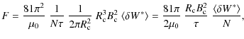
where N is the average number of steps taken to reach the threshold,
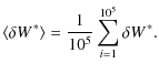
For the ensemble case,
4.2.3 Random walk step size
So far, we have assumed photospheric motions to be somewhat temporally incoherent, with a short random walk step,
![]() ,
corresponding to
,
corresponding to ![]() s.
Here, we consider the effect of varying this step length; in other
words, varying the coherence time of the photospheric motions.
Figure 15, which should be compared with the bottom right panel of Fig. 14, shows the distributions that result when
s.
Here, we consider the effect of varying this step length; in other
words, varying the coherence time of the photospheric motions.
Figure 15, which should be compared with the bottom right panel of Fig. 14, shows the distributions that result when
![]() is increased by factors of 10 and 40. For the latter case, the step is
sufficiently long that, on average, just one step is required to reach
the instability threshold: this corresponds to a temporally coherent
twisting of the loop (although the spatial profile of the twisting
varies randomly between heating events).
is increased by factors of 10 and 40. For the latter case, the step is
sufficiently long that, on average, just one step is required to reach
the instability threshold: this corresponds to a temporally coherent
twisting of the loop (although the spatial profile of the twisting
varies randomly between heating events).
| Figure 15:
Flare energy distributions over 105 relaxation events for a step size of
|
|
| Open with DEXTER | |
It can be seen that the energy distribution is virtually independent of the random walk step size. However, the heating flux does depend on this quantity. It is expected that the heating flux should be proportional to ![]() (Berger 1991; Zirker & Cleveland 1993). Equation (28) shows this to be the case, since the average number of steps, N, for the random walk to reach the threshold scales as
(Berger 1991; Zirker & Cleveland 1993). Equation (28) shows this to be the case, since the average number of steps, N, for the random walk to reach the threshold scales as
![]() .
In particular, if we consider the limiting case of coherent twisting (
.
In particular, if we consider the limiting case of coherent twisting (![]() s,
s,
![]() and
and
![]() )
we find that the flux increases significantly,
)
we find that the flux increases significantly,
![]() erg cm-2 s-1 for Active Regions.
erg cm-2 s-1 for Active Regions.
4.2.4 Random walks in twist space
The instability threshold can be expressed in terms of
![]() and
and
![]() ). This is more representative of the twist profile (see Sect. 3), which is directly generated by photospheric motions. We use
). This is more representative of the twist profile (see Sect. 3), which is directly generated by photospheric motions. We use
![]() and
and
![]() to obtain a 2-parameter representation of the family
to obtain a 2-parameter representation of the family
![]() ,
since the twist profiles of Fig. 4 usually show peak twists at the radial boundaries
,
since the twist profiles of Fig. 4 usually show peak twists at the radial boundaries ![]() (0.5) and
(0.5) and ![]() (1.0). The instability threshold can thus be plotted in twist space rather than alpha space, as in Fig. 3.
Given that the process is driven by turbulent photospheric motions, it
is more realistic to consider that the twist randomly evolves, rather
than the
(1.0). The instability threshold can thus be plotted in twist space rather than alpha space, as in Fig. 3.
Given that the process is driven by turbulent photospheric motions, it
is more realistic to consider that the twist randomly evolves, rather
than the ![]() profile. We thus repeat our calculations with a random walk in
profile. We thus repeat our calculations with a random walk in ![]() -space.
-space.
| Figure 16:
The instability threshold and relaxation line in |
|
| Open with DEXTER | |
When a simulation is run, for a sequence of heating events, in ![]() -space, the resulting energy profile is more or less identical to that generated by an
-space, the resulting energy profile is more or less identical to that generated by an ![]() -space simulation, see Fig. 16 (right). The translation to
-space simulation, see Fig. 16 (right). The translation to ![]() -space
results in a slight reorientation of the relaxation line with respect
to the threshold. Consequently, the relaxation line is closer to the
part of the threshold associated with the highest energies; this
explains why the distribution has a thicker tail. The energy flux is
-space
results in a slight reorientation of the relaxation line with respect
to the threshold. Consequently, the relaxation line is closer to the
part of the threshold associated with the highest energies; this
explains why the distribution has a thicker tail. The energy flux is
![]() erg cm-2 s-1, which increases with step size in the same manner as shown for the
erg cm-2 s-1, which increases with step size in the same manner as shown for the ![]() -space simulations.
-space simulations.
4.3 Temporal properties
We can gain some insight into the temporal distribution of heating events by assuming that each step of a random walk in ![]() -space takes the same arbitrary unit of time, corresponding to photospheric driving. The time axes of Fig. 17 are shown in terms of random walk step number (i.e., step count or running step count). The time unit
-space takes the same arbitrary unit of time, corresponding to photospheric driving. The time axes of Fig. 17 are shown in terms of random walk step number (i.e., step count or running step count). The time unit ![]() is the time taken for one step, which was estimated to be 200 s, see Sect. 2.3.
is the time taken for one step, which was estimated to be 200 s, see Sect. 2.3.
![\begin{figure}
\par\mbox{\includegraphics[width=4.4cm,clip]{14067171}\hspace*{1m...
...173}\hspace*{1mm}
\includegraphics[width=4.4cm,clip]{14067174} }
\end{figure}](/articles/aa/full_html/2010/13/aa14067-10/img164.png)
|
Figure 17: Top left: the number of steps between relaxation and instability (i.e., time interval between heating events) for each event of a simulation comprising 104 events. Top right: the number of steps taken to reach the threshold against the energy released. Bottom left: the energy release as a function of time (running step count). Bottom right: the 105 event simulation produced 105 flares of varying energies. The size of the flares are shown in a way that is reminiscent of actual flare/microflare/nanoflare observations: the bigger the event, the wider the base of the triangle used to represent that flare. The figure covers a time sequence equal to 5000 steps, taken from a random position within the simulation data. |
| Open with DEXTER | |
The probability that a flare event will have occurred after a particular number of steps in ![]() -space is invariant with time, see Fig. 17
(top left). This is also true for the probability that a flare event
will have a particular energy: the flare energy is not dependent on
where in the simulation it occurs. The two horizontal bands shown in
the bottom left panel are consistent with the peaks shown in Figs. 14, 15.
-space is invariant with time, see Fig. 17
(top left). This is also true for the probability that a flare event
will have a particular energy: the flare energy is not dependent on
where in the simulation it occurs. The two horizontal bands shown in
the bottom left panel are consistent with the peaks shown in Figs. 14, 15.
There does appear to be a slight relationship between the flare interval time (i.e., the number of steps taken to reach the threshold) and the flare energy, see Fig. 17 (top right); but, no positive correlation is evident. Observations strongly suggest that these two properties are uncorrelated (Wheatland 2000). The top right panel echoes the shape of the energy release distributions. The instability threshold has an energy release gradient, which means that sections of threshold that have a more or less constant energy release (low gradient) will be visited by more loops. The higher the number of visiting loops, the wider the range of step counts associated with that section of the threshold. Thus, Fig. 17 (top right) is in agreement with observations.
Finally, the simulated energy releases can also be represented as a time series of flare energies, again see Fig. 17 (bottom left).
4.4 Critical magnetic shear and coronal heating requirements
Parker (1988) explains
that a magnetic flux bundle rooted in the photosphere (i.e., a coronal
loop) will be stressed as photospheric motions move the footpoints in a
direction transverse to the original magnetic field. The coronal
heating requirements for Active Regions and for the Quiet Sun can be
converted to equivalent magnetic stresses, which can in turn be
converted to magnetic shears (B![]() Bz);
Bz);
where B
Thus, for coronal heating to work, there must be some
mechanism which restricts the shear to around these levels. If
dissipation occurs at lower levels of shear the energy flux cannot
maintain coronal temperatures. Conversely, if the shear can build up to
much larger levels, the energy input would be higher than required. Our
model provides an explanation for these critical shear values. We
calculate two types of mean magnetic shear along the threshold, the
mean absolute shear and the root mean square shear:
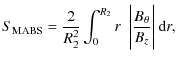
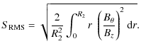
Both quantities are area-averaged. The plot (Fig. 18) shows that the values of S
| Figure 18: The mean absolute (solid) and root mean square (dashed) of the magnetic shear along the instability threshold. The shears are calculated over the loop volume, 0-R2. |
|
| Open with DEXTER | |
We should mention the work of Dahlburg et al. (2009), who provide an alternative explanation of this shear dependency involving an explosive ``secondary instability''. They have used a 3D viscoresistive MHD code to simulate the shearing of a line-tied flux tube. The results of this code have revealed that the secondary instability requires a critical shear for onset.
5 Summary and conclusions
We have used a model based on relaxation theory to determine the energy release of a sequence of heating events generated by random photospheric footpoint motions. This is a ``stress-relax'' scenario, in which free energy is continually built-up in the corona due to photospheric driving - repeated relaxations occur whenever a critical condition is reached. We postulate that heating events are triggered by the onset of an ideal kink instability. Energy release then occurs by fast magnetic reconnection in current sheets generated during the nonlinear phase of the instability, and this is calculated by assuming a helicity-conserving relaxation to a minimum energy state. The energy release of any individual heating event depends on the current profile at the point where the instability threshold is crossed - thus heating events of a range of sizes are found.
The initial stressed fields are modelled using piecewise-constant profiles of ![]() ,
yielding a two-parameter family of current profiles. Photospheric
driving thus yields a random walk of the current profile. In order to
pursue the calculation, the ideal instability threshold of a line-tied
loop has been determined. The modelled current profiles incorporate
regions of positive and negative twist as well as monotonic twist
profiles, as have been more commonly studied. We have shown that it is
not possible to determine the onset of instability by any simple
criterion such as achieving a critical twist or critical helicity.
Nevertheless, Fig. 4 suggests that the location of the instability is coincident with the peak twist (the largest absolute twist).
,
yielding a two-parameter family of current profiles. Photospheric
driving thus yields a random walk of the current profile. In order to
pursue the calculation, the ideal instability threshold of a line-tied
loop has been determined. The modelled current profiles incorporate
regions of positive and negative twist as well as monotonic twist
profiles, as have been more commonly studied. We have shown that it is
not possible to determine the onset of instability by any simple
criterion such as achieving a critical twist or critical helicity.
Nevertheless, Fig. 4 suggests that the location of the instability is coincident with the peak twist (the largest absolute twist).
A distribution of heating events has been calculated, both for the case
of a single loop which undergoes repeated stressing and relaxation, and
for an ensemble of identical loops which are randomly stressed (and for
intermediate cases). For a sufficiently large number of events, a
statistically-stable distribution of event sizes is obtained. As
expected, the smallest events are the most common, and there is (as
noted by Browning & Van der Linden 2003)
a minimum event size for given loop parameters, perhaps corresponding
to an ``elemental nanoflare''. More surprisingly, there is a second
peak of event frequency at intermediate magnitudes, although this is
somewhat reduced in size if an ensemble of loops is considered. This
can be explained as follows. The first peak (at minimum energy) occurs
simply because the range of energies near the minimum naturally
encompasses the largest part of the instability threshold curve
(because of the flatness of the minimum). The second peak is found
because the instability threshold is most likely to be crossed in the
part near to the region of constant-![]() .
.
An ensemble of identical loops - in which each individual loop starts from a randomly chosen initial state and is stressed until it undergoes a single relaxation event - is investigated in more detail. The distribution of heating events is qualitatively similar, although, the secondary peak of event frequency is much lower, and the decay of frequency with increasing energy is much flatter. A significant result is that, although the distribution is not a simple power law, the high-energy part of the distribution is well approximated by a power law with an index of around -8.3, which is considerably steeper than the minimum required for nanoflare heating to be effective (-2).
The model requires that the field is sometimes unstable -
although most of the time, the field profile will be well within the
stable region. Typically, the dimensional ![]() value is of magnitude 1-2, leading to dimensional values of
value is of magnitude 1-2, leading to dimensional values of
![]() -2 Mm-1
(for a loop radius of 1 Mm). Note that this is the maximum value
which could be found, and usually we would expect lower values. This is
consistent with observations; for example Régnier & Priest (2007) find
-2 Mm-1
(for a loop radius of 1 Mm). Note that this is the maximum value
which could be found, and usually we would expect lower values. This is
consistent with observations; for example Régnier & Priest (2007) find ![]() magnitudes around 1 Mm-1.
Furthermore, a consequence of the fact that the fields are predicted to
fluctuate between stable and unstable states is that we predict a value
for the average horizontal field component (on average, this will be
somewhat less than the value at marginal stability). At threshold, we
find B
magnitudes around 1 Mm-1.
Furthermore, a consequence of the fact that the fields are predicted to
fluctuate between stable and unstable states is that we predict a value
for the average horizontal field component (on average, this will be
somewhat less than the value at marginal stability). At threshold, we
find B![]() /Bz
is around 0.5, which means that its average value should be around
0.25. This agrees very well with the limit on this quantity required by
Parker (1988), in order for
the Poynting flux from the photosphere to match coronal heating
requirements. Hence, we have an explanation for the critical shear
value predicted by Parker. This also implies that the average heating
flux from our model will be sufficient for coronal heating. Indeed, the
fluxes derived from our results agree (especially if we raise the
correlation time for photospheric motions) with the required values.
/Bz
is around 0.5, which means that its average value should be around
0.25. This agrees very well with the limit on this quantity required by
Parker (1988), in order for
the Poynting flux from the photosphere to match coronal heating
requirements. Hence, we have an explanation for the critical shear
value predicted by Parker. This also implies that the average heating
flux from our model will be sufficient for coronal heating. Indeed, the
fluxes derived from our results agree (especially if we raise the
correlation time for photospheric motions) with the required values.
Relaxation theory makes no prediction about the spatial distribution of energy dissipation. However, this can be determined from numerical simulations. Recently, Hood et al. (2009) have shown that heating is well-distributed across the loop volume, as the current sheet, associated with the nonlinear kink instability, stretches and fragments, thereby filling the loop cross section. This has implications for the observed emission.
A further important consideration is that we study a single
loop of fixed dimensions, with repeated stressing and relaxation. In
practice, coronal heating events will occur in regions of field of
varying sizes. A large flare will inevitably involve a large magnetic
field volume, whereas nanoflares may involve small sets of fieldlines.
This could be accounted for in our model by allowing the loop radius to
be randomly distributed also; the effect would be to convolve a set of
our energy distributions. A second limitation of the calculation is
that we have assumed a uniform random walk in ![]() space. This is not realistic, since photospheric twisting motions are
likely to be correlated across the loop cross section and therefore
changes in which the twist in the outer later is similar to that in the
core are much more likely: in other words, there should be a positive
correlation between changes in
space. This is not realistic, since photospheric twisting motions are
likely to be correlated across the loop cross section and therefore
changes in which the twist in the outer later is similar to that in the
core are much more likely: in other words, there should be a positive
correlation between changes in ![]() (the core current) and changes in
(the core current) and changes in ![]() (the current in the outer layer), rather than these being independent
random variables as assumed here. This will be considered further in
future work.
(the current in the outer layer), rather than these being independent
random variables as assumed here. This will be considered further in
future work.
As well as the improvements mentioned above, the model will be enhanced such that there is, more realistically, zero net-current carried by the loop. At present, in most cases the potential layer outside the loop contains azimuthal field. A current neutralisation layer will be inserted between the loop and the envelope - external magnetic fields will have an axial direction only (Hood et al. 2009), representing a response to localised photospheric twist motions.
The model has included a number of simplifications, and at this stage is more of a ``proof of principle'' showing that a distribution of heating events can be produced from an (almost) ab initio coronal heating model. These initial results demonstrate the viability of the model for further research.
AcknowledgementsWe are grateful to Jim Klimchuk for helpful comments and M.R.B. thanks STFC for studentship support.
References
- Abramenko, V. I., Pevstov, A. A., & Romano, P. 2006, ApJ, 81, L646 [Google Scholar]
- Arber, T. D., Longbottom, A. W., & Van der Linden, R. A. M. 1999, ApJ, 517, 990 [NASA ADS] [CrossRef] [Google Scholar]
- Aschwanden, M. J., & Parnell, C. E. 2002, ApJ, 572, 1048 [NASA ADS] [CrossRef] [Google Scholar]
- Baty, H. 2000, A&A, 360, 345 [NASA ADS] [Google Scholar]
- Baty, H. 2001, A&A, 367, 321 [NASA ADS] [CrossRef] [EDP Sciences] [Google Scholar]
- Baty, H., & Heyvaerts, J. 1996, A&A, 308, 935 [NASA ADS] [Google Scholar]
- Berger, M. A. 1991, A&A, 252, 369 [NASA ADS] [Google Scholar]
- Berger, M. A. 1999, Plasma Phys. Control. Fusion, 41, B167 [NASA ADS] [CrossRef] [Google Scholar]
- Berger, M. A., & Field, G. B. 1984, J. Fluid. Mech., 147, 133 [Google Scholar]
- Browning, P. K., Sakurai, T., & Priest, E. R. 1986, A&A, 158, 217 [NASA ADS] [Google Scholar]
- Browning, P. K., & Van der Linden, R. A. M. 2003, A&A, 400, 355 [NASA ADS] [CrossRef] [EDP Sciences] [Google Scholar]
- Browning, P. K., Gerrard, C., Hood, A. W., Kevis, R., & Van der Linden, R. A. M. 2008, A&A, 485, 837 [NASA ADS] [CrossRef] [EDP Sciences] [Google Scholar]
- Dahlburg, R. B., Liu, J., Klimchuk, J. A., & Nigro, G. 2009, ApJ, 704, 1059 [NASA ADS] [CrossRef] [Google Scholar]
- Finn, J. M., & Antonsen, T. M. 1985, Communications in Plasma Physics and Controlled Fusion, 9, 111 [Google Scholar]
- Fletcher, L. 2009, A&A, 493, 241 [NASA ADS] [CrossRef] [EDP Sciences] [Google Scholar]
- Galsgaard, K., & Nordlund, A. 1997, J. Geophys. Res., 102 A1, 219 [Google Scholar]
- Gerrard, C. L., Arber, T. D., Hood, A. W., & Ven der Linden, R. A. M. 2001, A&A, 373, 1089 [NASA ADS] [CrossRef] [EDP Sciences] [Google Scholar]
- Heyvaerts, J., & Priest, E. R. 1984, A&A, 137, 63 [NASA ADS] [Google Scholar]
- Hollweg, J. V. 1984, ApJ, 277, 392 [NASA ADS] [CrossRef] [Google Scholar]
- Hood, A. W. 1992, Plasma Phys. Control. Fusion, 34, 411 [NASA ADS] [CrossRef] [Google Scholar]
- Hood, A. W., & Priest, E. R. 1979, Sol. Phys., 64, 303 [NASA ADS] [CrossRef] [Google Scholar]
- Hood, A. W., & Priest, E. R. 1981, Geophys. Astrophys. Fluid Dyn., 17, 297 [NASA ADS] [CrossRef] [Google Scholar]
- Hood, A. W., Browning, P. K., & Van der Linden, R. A. M. 2009, A&A, 506, 913 [NASA ADS] [CrossRef] [EDP Sciences] [Google Scholar]
- Hudson, H. S. 1991, Sol. Phys., 133, 357 [Google Scholar]
- Janse, Å. M., & Low, B. C. 2007, A&A, 472, 957 [NASA ADS] [CrossRef] [EDP Sciences] [Google Scholar]
- Klimchuk, J. A. 2006, Sol. Phys., 234, 41 [NASA ADS] [CrossRef] [Google Scholar]
- Krucker, S., & Benz, A. O. 1998, ApJ, 501, L213 [NASA ADS] [CrossRef] [Google Scholar]
- Kwon, R. Y., & Chae, J. 2008, ApJ, 677, L141 [NASA ADS] [CrossRef] [Google Scholar]
- Lionello, R., Velli, M., Einaudi, G., & Mikic, Z. 1998, ApJ, 494, 840 [NASA ADS] [CrossRef] [Google Scholar]
- Malanushenko, A., Longcope, D. W., Fan, Y., & Gibson, S. E. 2009, ApJ, 702, 580 [NASA ADS] [CrossRef] [Google Scholar]
- Melrose, D. B., Nicholls, J., & Broderick, N. G. 1994, J. Plasma Phys., 51, 163 [NASA ADS] [CrossRef] [Google Scholar]
- Mikic, Z., Schnack, D. D., & Van Hoven, G. 1990, ApJ, 361, 690 [NASA ADS] [CrossRef] [Google Scholar]
- Narain, U., & Ulmschieder, P. 1996, Space Sci. Rev., 75, 453 [NASA ADS] [CrossRef] [Google Scholar]
- Parker, E. N. 1988, ApJ, 330, 474 [Google Scholar]
- Parnell, C. E. 2004, Proceedings of the SOHO-15 Workshop ESA SP-575, ESA Pub. Div., Noordwijk, Holland, 227 [Google Scholar]
- Parnell, C. E., & Jupp, P. E. 2000, ApJ, 529, 554 [NASA ADS] [CrossRef] [Google Scholar]
- Porter, L. J., Klimchuk, J. A., & Sturrock, P. A. 1994, ApJ, 435, 482 [NASA ADS] [CrossRef] [Google Scholar]
- Portier-Fozzani, F., Aschwanden, M., Démoulin, P., Neupert, W., & Delaboudinière. 2001, Sol. Phys., 203, 289 [NASA ADS] [CrossRef] [Google Scholar]
- Priest, E. R. 1987, Solar Magnetohydrodynamics (Dordrecht, The Netherlands: D. Reidel Publishing Company) [Google Scholar]
- Priest, E. R., Longcope, D. W., & Heyvaerts, J. 2005, ApJ, 624, 1057 [NASA ADS] [CrossRef] [Google Scholar]
- Qiu, J. 2009, ApJ, 692 1110 [NASA ADS] [CrossRef] [Google Scholar]
- Régnier, S., & Priest, E.R. 2007, A&A, 468, 761 [Google Scholar]
- Sturrock, P. A., & Uchida, Y. 1981, ApJ, 246, 331 [NASA ADS] [CrossRef] [Google Scholar]
- Taylor, J. B. 1974, Phys. Rev. Lett., 33, 1139 [NASA ADS] [CrossRef] [Google Scholar]
- Taylor, J. B. 1986, Rev. Mod. Phys., 58, 741 [NASA ADS] [CrossRef] [Google Scholar]
- Van der Linden, R. A. M., & Hood, A. W. 1999, A&A, 346, 303 [NASA ADS] [Google Scholar]
- Vekstein, G. E., Priest, E. R., & Steele, C. D. C. 1993, ApJ, 417, 781 [NASA ADS] [CrossRef] [Google Scholar]
- Velli, M., Einaudi, G., & Hood, A. W. 1990, ApJ, 350, 428 [NASA ADS] [CrossRef] [Google Scholar]
- Velli, M., Lionello, R., & Einaudi, G., 1997, Sol. Phys., 172, 257 [NASA ADS] [CrossRef] [Google Scholar]
- Wheatland, M. S. 2000, Sol. Phys., 191, 381 [Google Scholar]
- Withbroe, G. L., & Noyes, R. W. 1977, Ann. Rev. Astr. Ap., 15, 363 [Google Scholar]
- Woltjer, L. 1958, Proc. Natl. Acad. Sci., USA, 44, 489 [Google Scholar]
- Zhang, M., & Low, B. C. 2003, ApJ, 584, 479 [NASA ADS] [CrossRef] [Google Scholar]
- Zirker, J. B., & Cleveland, F. M. 1993, Sol. Phys., 144, 341 [NASA ADS] [CrossRef] [Google Scholar]
Online Material
Appendix A: Expressions for loop properties
Expressions for some key quantities (
![]() ,
K and W) are given here. For compactness, these are given only for
,
K and W) are given here. For compactness, these are given only for
![]() and
and
![]() ,
while special cases (e.g.,
,
while special cases (e.g.,
![]() )
must be dealt with separately. Expressions for constant-
)
must be dealt with separately. Expressions for constant-![]() fields can be recovered by setting
fields can be recovered by setting
![]() ,
which gives more familiar formulae. The superscripts and subscripts
that accompany each quantity term denote the upper and lower radial
bounds over which the quantity is calculated.
,
which gives more familiar formulae. The superscripts and subscripts
that accompany each quantity term denote the upper and lower radial
bounds over which the quantity is calculated.
A.1 Average magnetic twist
| |
= | ![$\displaystyle \frac{\sigma_1 L\Big[1-J_0(\vert\alpha_1\vert R_1)\Big]}{R_1 J_1(\vert\alpha_1\vert R_1)}$](/articles/aa/full_html/2010/13/aa14067-10/img180.png)
|
(A.1) |
| = | ![$\displaystyle \frac{\sigma_2 L\Big[F_0(\vert\alpha_2\vert R_1)-F_0(\vert\alpha_...
...ig]}{\Big[R_2 F_1(\vert\alpha_2\vert R_2)-R_1 F_1(\vert\alpha_2\vert R_1)\Big]}$](/articles/aa/full_html/2010/13/aa14067-10/img182.png)
|
(A.2) | |
| = | ![$\displaystyle \frac{2\sigma_2 L R_2\Big[B_2 J_1(\vert\alpha_2\vert R_2) + C_2 Y...
...{R_2}\Big)}{B_2 F_0(\vert\alpha_2\vert R_2)\Big[R_3^{~2} - R_2^{~2}\Big]} \cdot$](/articles/aa/full_html/2010/13/aa14067-10/img184.png)
|
(A.3) |
A.2 Magnetic helicity
| K0R1 | = | 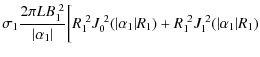
|
|
![$\displaystyle -2\frac{R_1}{\vert\alpha_1\vert}J_0(\vert\alpha_1\vert R_1)J_1(\vert\alpha_1\vert R_{1})\bigg]$](/articles/aa/full_html/2010/13/aa14067-10/img186.png)
|
(A.4) | ||
| KR1R2 | = | 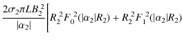
|
|
![$\displaystyle \times\Bigg(\frac{1}{\vert\alpha_1\vert}-\frac{\sigma_{1,2}}{\vert\alpha_2\vert}\Bigg)\Bigg]$](/articles/aa/full_html/2010/13/aa14067-10/img192.png)
|
(A.5) |
![\begin{displaymath}K_{R_2}^{R_3} \!= \! 2\sigma_2 L C_3 R_2\Bigg[\Big(\psi_{R_2}...
... \!\frac{\pi B_3}{2}\Big(R_3^{2} \!-\! R_2^{2}\Big)\Bigg]\cdot
\end{displaymath}](/articles/aa/full_html/2010/13/aa14067-10/img193.png)
|
(A.6) |
A.3 Magnetic energy
| W0 R1 | = | 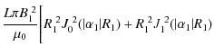
|
|
![$\displaystyle -\frac{R_1}{\vert\alpha_1\vert}J_0(\vert\alpha_1\vert R_1)J_1(\vert\alpha_1\vert R_1)\Bigg]$](/articles/aa/full_html/2010/13/aa14067-10/img195.png)
|
(A.7) | ||
| WR1 R2 | = | 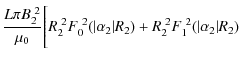
|
|
![$\displaystyle +\frac{R_1}{\vert\alpha_2\vert}F_0(\vert\alpha_2\vert R_1)F_1(\vert\alpha_2\vert R_1)\Bigg]$](/articles/aa/full_html/2010/13/aa14067-10/img199.png)
|
(A.8) | ||
| WR2 R3 | = | ![$\displaystyle ~\frac{L\pi}{\mu_0}\Bigg[\frac{B_3^{~2}}{2}\bigg(R_3^{~2} - R_2^{~2}\bigg) + C_3^{~2} R_2^{~2}\log\Bigg(\frac{R_3}{R_2}\Bigg)\Bigg]\cdot$](/articles/aa/full_html/2010/13/aa14067-10/img200.png)
|
(A.9) |
Appendix B: Magnetic field profiles for a selection of  -space points
![\begin{figure}
\par\includegraphics[width=9cm,clip]{14067-figb1.eps}
\end{figure}](/articles/aa/full_html/2010/13/aa14067-10/img201.png)
|
Figure B.1:
The magnetic field profiles, Bz (solid) and B |
| Open with DEXTER | |
Footnotes
- ... instability
- Appendices are only available in electronic form at http://www.aanda.org
All Figures
|
|
Figure 1:
Schematic of a straightened coronal loop in the r- |
| Open with DEXTER | |
| In the text | |
| |
Figure 2:
The left panel shows the closed instability threshold (solid) with the Bz reversal lines (dashed). The top half of the threshold (where
|
| Open with DEXTER | |
| In the text | |
|
|
Figure 3:
The instability threshold encloses the relaxation line, which is a subsection of the |
| Open with DEXTER | |
| In the text | |
|
|
Figure 4: The loop's radial twist profile at specific points along the threshold (labelled A-F). |
| Open with DEXTER | |
| In the text | |
| |
Figure 5:
The linear eigenfunction, Vx(x,
|
| Open with DEXTER | |
| In the text | |
| |
Figure 6:
The linear eigenfunction, Vx(x,
|
| Open with DEXTER | |
| In the text | |
| |
Figure 7:
The linear eigenfunction, Vx(x,
|
| Open with DEXTER | |
| In the text | |
|
|
Figure 8:
The variation in magnetic twist around the instability threshold (the threshold points are defined in Fig. 2) for three radial positions. The solid line represents the variation in axial twist, |
| Open with DEXTER | |
| In the text | |
|
|
Figure 9:
The variation in the average twist over the core, 0-R1 (top left), the outer layer, R1-R2 (top right), the loop, 0-R2 (bottom left) and the loop and envelope, 0-R3 (bottom right). The solid lines were calculated according to Eq. (24); the dashed according to Eq. (23) and the long-short dashed according to Eq. (22). Again, the twist values are plotted in units of |
| Open with DEXTER | |
| In the text | |
|
|
Figure 10:
The variation in K/ |
| Open with DEXTER | |
| In the text | |
|
|
Figure 11:
Helicity (top left), magnetic energy (top right), relaxed alpha (bottom left) and energy release (bottom right) along the 1D representation of the instability threshold. The energies, W* and |
| Open with DEXTER | |
| In the text | |
|
|
Figure 12: Flare energy distributions for 100 ( top left), 1000 ( top right), 104 ( bottom left) and 105 ( bottom right) relaxation events. |
| Open with DEXTER | |
| In the text | |
|
|
Figure 13: The flare energy distribution for 105 relaxation events and the instability threshold (with relaxation line). All lines are colour-coded according to energy release. |
| Open with DEXTER | |
| In the text | |
|
|
Figure 14: Flare energy distributions over 105 relaxation events for a variety of loop lifetimes. The lifetimes are 1000 relaxation events (top left), 100 relaxation events (top right), 10 relaxation events (bottom left) and 1 relaxation event (bottom right). |
| Open with DEXTER | |
| In the text | |
| |
Figure 15:
Flare energy distributions over 105 relaxation events for a step size of
|
| Open with DEXTER | |
| In the text | |
| |
Figure 16:
The instability threshold and relaxation line in |
| Open with DEXTER | |
| In the text | |
|
|
Figure 17: Top left: the number of steps between relaxation and instability (i.e., time interval between heating events) for each event of a simulation comprising 104 events. Top right: the number of steps taken to reach the threshold against the energy released. Bottom left: the energy release as a function of time (running step count). Bottom right: the 105 event simulation produced 105 flares of varying energies. The size of the flares are shown in a way that is reminiscent of actual flare/microflare/nanoflare observations: the bigger the event, the wider the base of the triangle used to represent that flare. The figure covers a time sequence equal to 5000 steps, taken from a random position within the simulation data. |
| Open with DEXTER | |
| In the text | |
| |
Figure 18: The mean absolute (solid) and root mean square (dashed) of the magnetic shear along the instability threshold. The shears are calculated over the loop volume, 0-R2. |
| Open with DEXTER | |
| In the text | |
|
|
Figure B.1:
The magnetic field profiles, Bz (solid) and B |
| Open with DEXTER | |
| In the text | |
Copyright ESO 2010
Current usage metrics show cumulative count of Article Views (full-text article views including HTML views, PDF and ePub downloads, according to the available data) and Abstracts Views on Vision4Press platform.
Data correspond to usage on the plateform after 2015. The current usage metrics is available 48-96 hours after online publication and is updated daily on week days.
Initial download of the metrics may take a while.