Age and metallicity of star clusters in the Small Magellanic Cloud from integrated spectroscopy

B. Dias; P. Coelho; B. Barbuy; L. Kerber; T. Idiart

doi:10.1051/0004-6361/200912894

Home

All issues

Volume 520 (September-October 2010)

A&A, 520 (2010) A85

Full HTML

Free Access

Issue		A&A Volume 520, September-October 2010


Article Number		A85
Number of page(s)		17
Section		Stellar atmospheres
DOI		https://doi.org/10.1051/0004-6361/200912894
Published online		07 October 2010

A&A 520, A85 (2010)

Age and metallicity of star clusters in the Small Magellanic Cloud from integrated spectroscopy

B. Dias¹ - P. Coelho² - B. Barbuy¹ - L. Kerber^1,3 - T. Idiart¹

1 - Universidade de São Paulo, Dept. de Astronomia, Rua do Matão 1226, São Paulo 05508-090, Brazil
2 - Núcleo de Astrofísica Teórica - Universidade Cruzeiro do Sul, R. Galvão Bueno, 868, sala 105, Liberdade, 01506-000, São Paulo, Brazil
3 - Universidade Estadual de Santa Cruz, Rodovia Ilhéus-Itabuna km16, 45662-000 Ilhéus, Bahia, Brazil

Received 15 July 2009 / Accepted 17 April 2010

Abstract
Context. Analysis of ages and metallicities of star clusters in the Magellanic Clouds provide information for studies on the chemical evolution of the Clouds and other dwarf irregular galaxies.
Aims. The aim is to derive ages and metallicities from integrated spectra of 14 star clusters in the Small Magellanic Cloud, including a few intermediate/old age star clusters.
Methods. Making use of a full-spectrum fitting technique, we compared the integrated spectra of the sample clusters to three different sets of single stellar population models, using two fitting codes available in the literature.
Results. We derive the ages and metallicities of 9 intermediate/old age clusters, some of them previously unstudied, and 5 young clusters.
Conclusions. We point out the interest of the newly identified as intermediate/old age clusters HW1, NGC 152, Lindsay 3, Lindsay 11, and Lindsay 113. We also confirm the old ages of NGC 361, NGC 419, Kron 3, and of the very well-known oldest SMC cluster, NGC 121.

Key words: Magellanic Clouds - galaxies: dwarf - galaxies: star clusters - stars: abundances - stars: fundamental parameters

1 Introduction

The Small Magellanic Cloud (SMC) is classified as a dwarf irregular galaxy (dI), with an absolute magnitude of $M_{\rm V}$ $\approx$ -16.2 (Binney & Merrifield 1998), among a variety of other types of dwarf galaxies in the Local Group (see Tolstoy et al. 2009). The star formation history and chemical evolution of the SMC can only be understood by deriving ages and metallicities of its stellar populations.

Globular clusters in the Milky Way are all old, and the Large Magellanic Cloud (LMC) shows a well-known age gap, with no clusters between the ages of 4 and 10 Gyr (except for ESO 121-SC03), as first revealed by Jensen et al. (1988) and reconfirmed since then (e.g. Balbinot et al. 2010, and references therein). Therefore the SMC appears as a unique nearby dwarf galaxy that has star clusters of all ages and a wide range of metallicities; yet, they are still poorly studied. For example, Parisi et al. (2009) point out that their spectroscopic study of CaII triplet metallicities of 16 SMC clusters is the largest spectroscopic survey of these objects in the SMC.

Ages and metallicities of star clusters in external galaxies beyond the Local Group can only be derived from their integrated spectra with current observing facilities. In contrast, due to its proximity, the stellar populations of the Magellanic Clouds (MCs) can be studied through resolved colour-magnitude diagrams (CMDs) and spectroscopy of bright individual stars, HII regions, or planetary nebulae.

High-resolution abundance analyses of field individual supergiants in the SMC, among which the largest samples can be found in Hill et al. (1997) for K-type stars, Luck et al. (1998) for Cepheids, and Venn (1999) for A-type stars, were shown by Tolstoy et al. (2009) to be compatible with other dIs of the Local Group. Spectroscopy of HII regions in the SMC were carried out by Garnett et al. (1995), where objects with 7.3 < log (O/H) + 12 < 8.4 were studied. Spectroscopic abundances of a large sample of SMC planetary nebulae were presented in Idiart et al. (2007), where objects with 6.69 < log (O/H) + 12 < 8.51 were studied.

Ages of star clusters in the SMC using CMDs can now be obtained with improved angular resolutions, reaching several magnitudes below the turn-off, with higher accuracy (e.g., Glatt et al. 2008a,b, and references therein). De Grijs & Goodwin (2008) made use of the UBVR survey of the Clouds by Massey (2002), to derive relative ages and masses of stars clusters in the SMC, where we see that there are few star clusters with ages of 1 Gyr and older. Hill & Zaritsky (2006) presented structural parameters for 204 star clusters, and Glatt et al. (2009) give structural parameters for 23 intermediate/old age star clusters in the SMC. Chemical abundances from high-resolution spectra, on the other hand, are only available for two globular clusters, the young NGC 330 (Hill 1999; Gonzalez & Wallerstein 1999, and references therein) and the old NGC 121 (Johnson et al. 2004), the latter however only as preliminary work. Other high or mid resolution spectra are essentially only found for hot stars in young clusters or from surveys of the CaT triplet lines (e.g. Parisi et al. 2009; Da Costa & Hatzidimitriou 1998).

Recent work on the star formation history (SFH) of the SMC, based on large samples of field stars, have shown that its SFH is rather smooth and well-understood, as described in Dolphin et al. (2001), Harris & Zaritsky (2004), and Carrera et al. (2008). Dolphin et al. (2001) studied the SFH in a field around the old cluster NGC 121. A broadly peaked SFH is seen, with a high rate between 5 and 8 Gyr ago. Constant star formation from $\sim$ 15 to $\sim$ 2 Gyr ago could be adopted as well within 2 $\sigma$ . The metallicity increased from the early value of [Fe/H] $\approx$ -1.3 for ages above 8 Gyr, to [Fe/H] = -0.7 presently.

Harris & Zaritsky (2004), based on a UBVI catalogue of 6 million stars located in 351 SMC regions (Zaritsky et al. 1997), found similar evidence regarding the SMC's SFH. They suggest the following main characteristics: a) a significant epoch of star formation with ages older than 8.4 Gyr; b) a long quiescent epoch between 3 and 8.4 Gyr; c) a continuous star formation started 3 Gyr until the present; d) in period c), 3 main peaks of star formation should have occurred at 2-3 Gyr, 400 Myr, and 60 Myr. De Grijs & Goodwin (2008) claim to confirm the findings by Gieles et al. (2007), according to which there is little cluster disruption in the SMC, and therefore star clusters should be reliable tracers of star formation history, together with field stars.

We present the analysis of 14 star clusters, several of which still have very uncertain age and metallicity determinations. Our sample includes candidates to be of intermediate/old age.

We use the full-spectrum fitting codes S TARLIGHT (Cid Fernandes et al. 2005) and ULySS (Koleva et al. 2009) to compare, on a pixel-by-pixel basis, the integrated spectrum of the clusters to three sets of simple stellar population (SSP) models in order to derive their ages and metallicities. This technique is an improvement over older methods (e.g., the Lick/IDS system of absorption line indices, Worthey et al. 1994) and has been recently validated in Koleva et al. (2008); Cid Fernandes & Gonzalez Delgado (2010) and references therein. If integrated spectra can be proved to define reliable ages and metallicities, the technique can then be applied to other faint star clusters in the MCs, and in other external galaxies. As a check of our method, we compare our results to those from CMD analyses or other techniques available for the sample clusters. Previously we observed spectra for 14 clusters (6 in the SMC and 8 in the LMC), and we analysed them based on single stellar population models of integrated colours, as well as of H $\beta$ and $\langle$ Fe $\rangle$ spectral indices (de Freitas Pacheco et al. 1998).

We selected our sample from Sagar & Pandey (1989) (L3, K3, L11 and L113), Hodge & Wright (1974) and Hodge (1983) (HW 1, NGC 152, NGC 361, NGC 419, and NGC 458), and the well-known NGC 121. Young clusters were also included in the sample (NGC 222, NGC 256, NGC 269, and NGC 294) for comparison purposes. Our main aim is to identify intermediate/old star clusters in our sample. We assume that ``intermediate/old age'' populations are older than the Hyades (700 Myr, Friel 1995), as commonly adopted in our Galaxy.

In Sect. 2 we describe the observations and data reduction. In Sect. 3 we present the stellar population analysis. In Sect. 4 we discuss the results obtained. In Sect. 5 we comment on each cluster. Concluding remarks are given in Sect. 6.

2 Observations

Observations were carried out at the 1.60 m telescope of the National Laboratory for Astrophysics (LNA/MCT, Brazil) and at the 1.52 m telescope of the European Southern Observatory (ESO, La Silla, Chile). At the LNA, an SITe CCD camera of 1024 $\times$ 1024 pixels was used, with pixel size of 24 $\mu$ m. A 600 l/mm grating allowed a spectral resolution of 4.5 Å FWHM. Spectra were centered at Mgb $\lambda$ 5170, including the indices H $\beta$ $\lambda$ 4861, Fe $\lambda$ $\lambda$ 5270, 5335, Mg₂, and NaD $\lambda$ 5893. At ESO, a Loral/Lesser CCD camera #38, of 2688 $\times$ 512 pixels with pixel size of 15 $\mu$ m and a grating of 600 l/mm were used, allowing a spectral resolution of 4 Å FWHM.

We used long east-west slits in all observations (3 arcmin at LNA and 4.1 arcmin at ESO). For each cluster, from 2 to 6 individual measures were taken, mainly covering its brightest region. Integration times range from 20 to 50 min each, and we used slits of 2 arcsecs width in both observatories.

We used the IRAF package for data reduction, following the standard procedure for longslit CCD spectra: correction of bias, dark and flat-field, extraction, wavelength, and flux calibration. For flux calibration, we observed at least three spectrophotometric standard stars each night. Standard stars were observed in good sky conditions, with wider slits to ensure the absolute flux calibration. In some nights weather conditions were not photometric; however, even in these nights we observed spectrophotometric standards in order to secure a relative flux calibration. Atmospheric extinction was corrected through mean coefficients derived for each observatory. After reduction we combined the spectra to increase global S/N and filtered in order to minimise high-frequency noise, lowering their resolutions to about 7 Å FWHM. Table 1 presents the log of observations. Reddening values E(B-V) given in Table 1 were obtained by using the reddening maps of Schlegel et al. (1998). S/N ratios per pixel measured on the final spectra are also reported in Table 1.

Table 1: Log of observations.

3 Stellar population analysis

3.1 Literature data

Literature data available for the sample clusters are reported in Table 2. Values of reddening E(B-V), metallicity and age are listed, together with the corresponding references. The metallicity value is either the iron abundance [Fe/H] or the overall metallicity relative to solar [M/H] = [ $Z/Z_{\odot}$ ] = [Z], indicated by superscript 1 or 2, respectively. We assumed $Z_{\odot}$ = 0.017 for the cases where only the Z value was provided. Table 2 shows that there is very little information for most clusters. We can see that ages for some of them vary by several Gyr.

The spatial distribution of the 14 sample SMC clusters is shown in Fig. 1, where the sample clusters are projected over the location of SMC star clusters as given in Bica & Schmitt (1995). As can be seen in this figure, only one cluster (Lindsay 113) is located in the direction of the Bridge (east side), whereas the others are spread over the bulk of the clusters and mainly on the west side of the SMC.

In Table 3 we report the literature values adopted throughout the text, selected by weighting more reliable methods or data quality. In this table we also report estimated cluster masses. We estimated the masses of the clusters based on the SSP evolution models by Schulz et al. (2002). In their Fig. 8 values of V-band mass-to-light ratios (M/L_V) are plotted against age for three different metallicities ([ $Z/Z_{\odot}$ ] = -1.63, -0.33, 0.07). The M/L_V ratios were estimated by considering IMF prescriptions by either Salpeter (1955) or Scalo (1986), following calculations by Schulz et al. (2002). V-band luminosity was calculated adopting V magnitudes from SIMBAD and a common distance modulus of (m-M) = 18.9 (average value calculated from literature by NED website). For the clusters HW 1, Lindsay 3 and 113, the V magnitudes were not found, therefore we did not calculate their masses.

$\begin{figure} \par\includegraphics[width=7cm,clip]{12894fg1.ps} \end{figure}$	Figure 1: Distribution on the sky of the 14 SMC clusters analysed in this work (large full circles) overplotted on the star clusters listed in (Bica & Schmitt 1995) (small green circles).
Open with DEXTER

Table 2: Parameters from the literature.

3.2 Full spectrum fitting

We obtained ages and metallicities for the sample clusters through the comparison of their integrated spectrum to SSP models available in the literature. Modern techniques of spectral fitting allow comparison of observations and models on a pixel-by-pixel basis, and we adopted the public codes S TARLIGHT and ULySS, described briefly below.

S TARLIGHT (Cid Fernandes et al. 2005) is a multi-purpose code that combines N spectra from a user-defined base (in our case, SSP models from literature, characterized by age and [Fe/H]) in search for the linear combination which best matches an input observed spectrum. A S TARLIGHT run returns the best population mixture that fits the observed spectrum, in the form of the light fraction contributed by each of the SSPs in the base. It also returns (i) an estimation of the extinction A_V; (ii) the percentage mean deviation over all fitted pixels $\bar{\Delta} = \mid O_{\lambda} - M_{\lambda}\mid\!\!/O_{\lambda}$ (where $O_{\lambda}$ and $M_{\lambda}$ are the observed and the model spectra, respectively); (iii) $\chi^2_{\rm red}$ (reduced chi-square); of both the global fit; and (iv) the fits to each of the SSPs in the base models.

The use of S TARLIGHT to study the integrated spectra of clusters has been extensively discussed in Cid Fernandes & Gonzalez Delgado (2010). It is generally accepted that the majority of stellar clusters can be represented by a SSP, ideally only one component (SSP model) in the base would have a non-zero contribution. In practice, however, a multi-component fit may be returned by the code if (i) the parameters coverage of the base models is coarse; (ii) there is contamination from background or foreground field stars; (iii) the S/N is low; and/or (iv) if any stellar evolution phase present in the population is lacking in the models (as studied e.g. in Ocvirk 2010). We adopted as results the mean parameters of the fit (instead of the SSP chi-square selection as in Cid Fernandes & Gonzalez Delgado 2010), as a way to compensate for the coarseness of the parameters coverage of the SSP models. The results are then given by

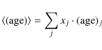
$\begin{displaymath}% \langle({\rm age})\rangle = \sum_{j}{x_j \cdot ({\rm age})_j} \end{displaymath}$

(1)

and

$\begin{displaymath}% \langle[Z/Z_{\odot}]\rangle = \sum_{j}{x_j \cdot [Z/Z_{\odot}]_j} \end{displaymath}$

(2)

where x_j gives the normalized light-fraction of the jth SSP component of the model fit ( $\sum_{j}{{\vec x}_j}=1$ ).

ULySS (Koleva et al. 2009) is a software package performing spectral fitting in two astrophysical contexts: the determination of stellar atmospheric parameters and the study of the star formation and chemical enrichment history of galaxies. In ULySS, an observed spectrum is fitted against a model (expressed as a linear combination of components) through a non-linear least-squares minimization. In the case of our study, the components are SSP models (the same as the base models for S TARLIGHT). The grid of SSPs is spline-interpolated to provide a continuous function. We used the procedures in the package yielding the SSP-equivalent parameters for a given spectrum, and adopted the values in Table 3 as initial guesses. We noticed that the use of adequate initial guesses increases the accuracy (and the homogeneity among different SSP models) of the derived parameters, especially for metallicities (see discussion in Koleva et al. 2008). There is no equivalent to initial guesses in S TARLIGHT runs. Also in contrast with S TARLIGHT, which fits both the slope of the spectrum and spectral lines, ULySS normalises model and observation through a multiplicative polinomial in the model, determined during the fitting process. Therefore, ULySS is not sensitive to flux calibration, galactic extinction, or any other cause affecting the shape of the spectrum.

For the present study we adopted three sets of SSP models:

models by (Bruzual & Charlot 2003, hereafter BC03), based on STELIB stellar library (Le Borgne et al. 2003) and Bertelli et al. (1994) isochrones. The models cover ages in the range 10⁵ < t(yr) < 1.5 $\times$ 10¹⁰, metallicities 0.0001 < Z < 0.05, in the wavelength interval 320-950 nm (the medium resolution set of models), at FWHM $\sim$ 3 Å.
models by Le Borgne et al. (2004) (hereafter PEGASE-HR), based on ELODIE library (Prugniel & Soubiran 2001) and Bertelli et al. (1994) isochrones. The models cover ages and metallicities in the range 10⁷ < t(yr) < 1.5 $\times$ 10¹⁰, 0.0004 < Z < 0.05, and wavelength interval of 400-680 nm, at FWHM $\sim$ 0.55 Å.
preliminary models by Vazdekis et al. (2010) (see also Vazdekis et al. 2007), which are an extension of the models by Vazdekis (1999) using the MILES library (Sánchez-Blázquez et al. 2006) and isochrones by Girardi et al. (2000). The models cover ages 10⁸ < t(yr) < 1.5 $\times$ 10¹⁰, metallicities 0.0004 < Z < 0.03, and wavelength interval 350-740 nm, at FWHM $\sim$ 2.3 Å.

By fitting the data with three different sets of SSP models, we aim at a better handle on the uncertainties of the derived parameters, and possibly detect model dependencies.

4 Results and discussion

We reported in Tables 4 and 5 the ages and metallicities obtained from S TARLIGHT and ULySS fits, respectively. Individual fits are shown in Figs. A.1 to A.34 (for the sake of space, only fits with PEGASE-HR are presented).

In Figs. 2 and 3 we compare the results of the two codes. Figure 2 shows the ages obtained with ULySS in the abcissa and those from S TARLIGHT in ordinates, for the BC03, PEGASE-HR, and Vazdekis models, respectively. We use the least absolute deviation method for the linear fits because it is considered more robust than $\chi^2$ minimisation. Figure 3 shows the same plots for metallicities. In Fig. 2 we note that, with the exception of the runs with PEGASE-HR models, ages derived from the two codes show a high dispersion, but not a clear trend. In contrast, in the case of metallicities (Fig. 3), S TARLIGHT runs will result in higher metalliticies than ULYSS runs in the low metallicity tail, with the trend reversing at the high-metallicity tail. In both cases the dispersion is high, and a safe conclusion can only be reached with a larger sample.

Figures 4 and 5 compare the results between different models but the same code, for ages and metallicities, respectively. With the exception of the middle panel in Fig. 5, we see that differences are dominated by shifts, rather than showing a dependence with age and/or metallicity. Figures 2 to 5 seem to indicate that, while the use of different SSP models might introduce zero-point shifts in the derived parameters, the choice of fitting code might introduce a more complicated behaviour, dependent on the range of population parameters studied.

In Figs. 6 and 7 we show the comparison of our results with literature data (Table 2) for ages and metallicities, respectively. Literature data as reported in Table 3 are plotted vs. difference of age between literature and the result from S TARLIGHT (panel a) and ULySS (panel b) (given in Gyr). Figure 7 shows the same for metallicity. In Table 6 we report a list of reliable ages and metallicities for well-known and/or well studied clusters, by trying to select mostly intermediate/old age ones. The list of clusters is basically that of Carrera et al. (2008), de Freitas Pacheco et al. (1998), Glatt et al. (2008a,b), Bica et al. (2008), Glatt et al. (2009), and Parisi et al. (2009). Figure 8 gives the age and metallicity of literature data for well-studied clusters, as reported in Table 6, and the results for our sample clusters derived with ULySS+PEGASE-HR. As discussed for example in Da Costa & Hatzidimitriou (1998), we see a relatively rapid rise in metallicity in the first 3 to 5 Gyr (assuming that chemical evolution started at 15 Gyr), and a slow increase in the metallicity from [Fe/H] $\approx$ -1.1 to -1.3 to the present value of [Fe/H] $\approx$ -0.7. We also overplot the chemical evolution model for the SMC computed by Pagel & Tautvaisiene (1998). The model fits the confirmed literature data well, as also found in previous work, and our results are compatible with the model and literature data.

Table 3: Values adopted from the literature (Table 2) for the clusters studied in this work, where masses are estimated based on models by Schulz et al. (2002).

Table 4: Best-fit results using S TARLIGHT.

Table 5: Best-fit results using ULySS.

$\begin{figure} \par\includegraphics[width=17.5cm,clip]{12894fg2.ps} \vspace*{3mm} \end{figure}$	Figure 2: Ages derived with S TARLIGHT and ULySS (Gyr) in each panel using a different SSP model: left panel: BC03, middle: PEGASE-HR, right panel: Vazdekis et al. The dashed lines are linear fits to the points using a least absolute deviation method and the dotted lines are the one-to-one match.
Open with DEXTER

$\begin{figure} \par\includegraphics[width=17.5cm,clip]{12894fg3.ps} \vspace*{3mm} \end{figure}$	Figure 3: Same as Fig. 2 for metallicities.
Open with DEXTER

$\begin{figure} \par\includegraphics[width=17.5cm,clip]{12894fg4.ps} \vspace*{5mm} \end{figure}$	Figure 4: Comparisons of ages derived with the three sets of SSPs (BC03, PEGASE-HR, Vazdekis). S TARLIGHT values are shown as blue circles, ULySS values as black squares. The dashed lines are linear fits to the points using a least absolute deviation method and the dotted lines are the one-to-one match.
Open with DEXTER

$\begin{figure} \par\includegraphics[width=17.5cm,clip]{12894fg5.ps} \vspace*{3mm} \end{figure}$	Figure 5: Same as Fig. 5 for metallicities.
Open with DEXTER

$\begin{figure} \par\includegraphics[width=7.5cm,clip]{12894fg6a.ps}\hspace{4mm} \includegraphics[width=7.5cm,clip]{12894fg6b.ps} \vspace{3mm} \end{figure}$	Figure 6: Ages from the literature (given in log age(yr)) from Table 3 in the abscissae vs. difference of age from literature and the result from S TARLIGHT and ULySS with the 3 SSPs, in the ordinate.
Open with DEXTER

$\begin{figure} \par\includegraphics[width=7.5cm,clip]{12894fg7a.ps}\hspace*{4mm} \includegraphics[width=7.5cm,clip]{12894fg7b.ps} \end{figure}$	Figure 7: Same as Fig. 6 for metallicities.
Open with DEXTER

$\begin{figure} \par\includegraphics[width=8.5cm,clip]{12894fg8.ps} \end{figure}$	Figure 8: Age-metallicity data for the sample clusters and selected literature data for well-known clusters. Symbols: filled circles: literature data (Table 6); filled triangles: present results based on S TARLIGHT+PEGASE-HR; filled squares: present results based on ULySS+PEGASE-HR. The chemical evolution model by Pagel & Tautvaisiene (1998) is overplotted.
Open with DEXTER

Table 6: Literature data of age and metallicity for well-known SMC star clusters.

5 Comments on individual clusters

Results obtained with S TARLIGHT and ULySS, given in Tables 4 and 5, for each cluster, are compared with previous analyses.

5.1 HW 1

There are no literature data on this cluster. From the analysis carried out with S TARLIGHT, we get an intermediate/old age and a low metallicity, whereas with ULySS, we get an old age and a low metallicity, and with both codes the results are consistent among the three sets of SSPs. The identification of such an old and metal-poor cluster is an important result. Preliminary CMD data obtained in our group indicate an age around 6 Gyr (to be published elsewhere), in better agreement with S TARLIGHT results.

5.2 Kron 3

Glatt et al. (2008a) derived an age of 6.5 Gyr, whereas Rich et al. (1984) find an age of 5-8 Gyr. The ages inferred are in most cases similar or older than the 6.5 Gyr expected. Low metallicities around [Fe/H] $\approx$ -1.6 are retrieved in all runs. High-resolution spectroscopy of individual stars of this cluster would be of great interest.

5.3 Lindsay 3

Kontizas (1980) subdivided a sample of 20 star clusters in young or old based on the colour of the nuclei of each cluster. By using this method, Lindsay 3 is 1 to 5 Gyr old, therefore an intermediate/old age cluster. Ages both from S TARLIGHT and ULySS give either around 1.5 or 7 Gyr. This cluster has among the lowest S/N in our sample, so this age discrepancy is not surprising. (Cid Fernandes & Gonzalez Delgado 2010, suggest a minimum of S/N $\sim$ 30 to obtain robust results.) Preliminary CMD analyses in our group, to be published elsewhere, give an age of 1-2 Gyr and metallicity of [Fe/H] $\approx$ -0.7. The S TARLIGHT and ULySS metallicities all agree that the cluster is metal-poor, likewise the CMD indications. L3 is revealed as an intermediate/old age and low metallicity cluster.

5.4 Lindsay 11

Kontizas (1980) gives and age in the range 1 to 5 Gyr based on CMDs. Both codes and the three SSPs give moderate metallicities within -0.8 < [Fe/H] < -0.5, in good agreement with Da Costa & Hatzidimitriou (1998). Ages of 5.1 to 8.9 Gyr are found with S TARLIGHT, whereas ULySS gives ages between 4.4 and 9.4. This could be an interesting cluster with an intermediate/old age around 5 Gyr.

5.5 Lindsay 113

Mighell et al. (1998) have derived and age of 4.7 Gyr (in the range of 4.0 < t(Gyr) < 5.3) and [Fe/H] = -1.24. S TARLIGHT and ULySS give low metallicities. The ages from S TARLIGHT are similar or older (for BC03) than Mighell et al. (1998)'s value, whereas a higher age dispersion is found with ULySS. This cluster of intermediate/old age is very promising and should be observed further.

5.6 NGC 121

Glatt et al. (2008a) obtained an HST/ACS CMD of NGC 121 and derived ages of 11.8, 11.2, and 10.5 Gyr based on Teramo (Pietrinferni et al. 2004), Padova (Girardi et al. 2000) and Dartmouth (Dotter et al. 2007) isochrones. In a final age scale, the authors adopt an age between 10.9 and 11.5 $\pm$ 0.5 Gyr. From our runs, metallicities in the range -1.7 < [Fe/H] < -1.3 are obtained. All ages are in the range 7.7 < t(Gyr) < 12. This well-known oldest cluster of the SMC could be a survivor of an epoch of a somewhat delayed first burst of cluster formation in the SMC (Glatt et al. 2008a).

5.7 NGC 152

For this cluster an age range of 1 to 5 Gyr is also given by Kontizas (1980). S TARLIGHT gives old ages of 7.5 to 10.9 Gyr and metallicities around [Fe/H] $\approx$ -1.1. ULySS gives young ages of 0.2 to 1.5 Gyr and very low metallicities of -2.3 < [Fe/H] < -1.4. For this cluster both the age and metallicity remain undefined, and it is clearly a good candidate for further studies on intermediate/old age clusters.

5.8 NGC 222

A young age of 100 Myr and [Fe/H] = -0.3 for NGC 222, were derived by employing isochrone fitting to VI CMDs by Chiosi et al. (2006). Young ages are obtained in all cases. On the other hand, low metallicities are derived in most cases and it remains undefined.

5.9 NGC 256

Chiosi et al. (2006) give 100 Myr and [Fe/H] = -0.3. S TARLIGHT gives similar results using BC03 and Vazdekis et al., whereas PEGASE-HR gives an intermediate age, with a metallicity similar to that derived by Chiosi et al. (2006). ULySS gives ages and metallicities in agreement with Chiosi et al. with the three SSP sets.

5.10 NGC 269

Chiosi et al. (2006) report 300 Myr and [Fe/H] = -0.3. ULySS gives results similar to Chiosi et al. values, with the 3 SSPs. S TARLIGHT gives metallicities -0.7 < [Fe/H] < -0.2, however BC03 and PEGASE-HR give intermediate ages.

5.11 NGC 294

Pietrzynski & Udalski (1999) present the CMD of NGC 294, and deriving an age of 0.33 $\pm$ 0.3 Gyr and a metallicity of [Fe/H] $\approx$ -0.6. The young age is confirmed in all runs. ULySS metallicities agree with the literature value, whereas S TARLIGHT runs give lower metallicities around [Fe/H] $\approx$ -1.2.

5.12 NGC 361

The NGC 361 CMD from Mighell et al. (1998) was cleaned of contaminations by field stars. There are two predominant populations: one older than the cluster that has similar CMD components, and the other one younger that has an extended main sequence. The cleaned cluster CMD shows clear RGB and HB sequences. Metallicities were derived from the CMDs using two methods and combining the results. The first method was the simultaneous fit of reddening and metallicity method (Sarajedini 1994), that depends on the magnitude level of the HB, the colour of the RGB at the level of the HB, and the shape and position of the RGB. The second one was the RGB slope method. A metallicity of [Fe/H] = -1.45 $\pm$ 0.11 was adopted. The method to determine the age was based on the colour of the red HB and the RGB at the level of the HB (Sarajedini et al. 1995) for a given metallicity, and an age of 6.8 $\pm$ 0.5 Gyr was adopted. They tried another method to derive relative ages with respect to Lindsay 1 and found 8.1 $\pm$ 1.2 Gyr. A population like this is clearly not well modelled by SSPs, and a challenge for spectral analysis such as the one presented here. Indeed an inspection of the multi-population fits returned by S TARLIGHT show superpositions of old ( $\sim$ 10 Gyr) and intermediate-age ( $\sim$ 2 Gyr) populations for this cluster. Nevertheless, the literature value of metallicity around $\sim$ -1.3 (see also Table 2) is confirmed in all combinations of code and SSPs. Ages are retrieved in a wide range, between 2.3 to 12.3 Gyr. S TARLIGHT+PEGASE-HR and ULySS+Vazdekis are the fits that better match Mighell et al. (1998) age results.

5.13 NGC 419

Using HST/ACS data, Glatt et al. (2008b) have recently demonstrated that NGC 419 is among the most interesting populous stellar clusters in the SMC due to the clear presence of multiple stellar populations with ages between $\sim$ 1.0 and ${\sim}2.0$ Gyr. This hypothesis was confirmed by a detailed analysis of this HST/ACS CMD performed by Girardi et al. (2009), which sustained the presence of multiple stellar populations not only by the main sequence spread, but also by a clear presence of a secondary clump. Furthermore, very recently Rubele et al. (2010) have recovered the SFH for this cluster, which lasts at least 700 Myr with a marked peak at the middle of this interval, for an age of 1.5 Gyr. Assuming the same chemical composition for all stars in NGC 419, these authors also determined a metallicity of [Fe/H] = -0.86 $\pm$ 0.09.

The same caveats of the previous cluster, on trying to fit SSPs to such a complex population, applies for this cluster as well. Even so, most combinations give satisfactory results, compatible with Glatt et al. (2008b). The older ages retrieved by S TARLIGHT+BC03, +PEGASE-HR could be due to the double turn-off found by Glatt et al. (2008b), where isochrones from 1 to 3 Gyr were fitted. ULySS gives ages and metallicities in agreement with Glatt et al. (2008b).

5.14 NGC 458

From integrated spectroscopy, Piatti et al. (2005b) give 130 Myr, and [Fe/H] = -0.23. Young ages are derived in all fits with the exception of S TARLIGHT+PEGASE-HR. Metallicity values show a rather large dispersion, confirming that uncertainties on this parameter are larger for young ages.

6 Conclusions

We observed mid-resolution integrated spectra of SMC star clusters to study the SMC chemical evolution and in particular to determine the stellar population parameters of intermediate/old age clusters. To study these integrated spectra, we exploited the ability of the codes S TARLIGHT and ULySS, coupled with Single Stellar Populations (SSPs) spectral models to derive their ages and metallicities. The SSPs models employed are those by BC03, Pegase-HR, and Vazdekis et al.

We highlight the importance of the intermediate/old age clusters HW1, L3, L11, NGC 152, NGC 361, NGC 419, and L113. We also confirm the intermediate/old age of Kron 3 and old age of NGC 121.

There seems to be an indication that the choice of the code will have more impact on the results than the choice of models. We point out that the S TARLIGHT results adopted are a mean of the main stellar populations identified, therefore some of the differences in the results relative to ULySS may result from this.

We also derived masses for the sample clusters, reported in Table 3. De Grijs & Goodwin (2008) published cluster mass functions based on statistically complete SMC cluster samples, and our results are compatible with their mass distribution (their Fig. 2, panel d), since we find that most clusters have masses around log( $M_{\rm cl}$ / $M_{\odot}$ ) $\sim$ 4.

Another interesting issue is the existence of very metal-poor stellar populations in the SMC. Planetary nebulae older than 1 Gyr show [Fe/H] > -1.0 $\pm$ 0.2 with very few exceptions (Idiart et al. 2007), whereas clusters analysed here show metallicities lower than [Fe/H] < -1.0. It would be particularly interesting to carry out high resolution spectroscopic analysis of individual stars in these clusters, in order to check if there are very metal-poor clusters, that apparently have no counterpart among the planetary nebulae population, or at least very few. The confirmation of metallicities of the most metal-poor planetary nebulae would be needed.

Finally we identified a few clusters with ages between 1 and 8 to 10 Gyr (upper limits vary between code and SSP employed in our calculations); therefore, we conclude that no clear age gap is present in the SMC.

Acknowledgements

P.C. is grateful to M. Koleva and P. Prugniel for the help with ULySS and to R. Cid-Fernandes for the long term help with S TARLIGHT. B.D., P.C., B.B., T.I. and L.K. acknowledge partial financial support from the Brazilian agencies CNPq and Fapesp. P.C. acknowledges the partial support of the EU through a Marie Curie Fellowship. The authors are grateful to an anonymous referee for very helpful suggestions. The observations were carried out within Brazilian time in a ESO-ON agreement and within an IAG-ON agreement funded by FAPESP project No. 1998/10138-8.

References

Ahumada, A. V., Clariá, J. J., Bica, E., & Dutra, C. M. 2002, A&A, 393, 855 [NASA ADS] [CrossRef] [EDP Sciences] [Google Scholar]
Alcaino, G., Liller, W., Alvarado, F., et al. 1996, AJ, 112, 2004 [NASA ADS] [CrossRef] [Google Scholar]
Balbinot, E., Santiago, B. X., Kerber, L. O., Barbuy, B., & Dias, B. M. S. 2010, MNRAS, 404, 1625 [NASA ADS] [Google Scholar]
Bertelli, G., Bressan, A., Chiosi, C., Fagotto, F., & Nasi, E. 1994, A&AS, 106, 275 [NASA ADS] [Google Scholar]
Bica, E. L. D., & Schmitt, H. R. 1995, ApJS, 101, 41 [NASA ADS] [CrossRef] [Google Scholar]
Bica, E., Dottori, H., & Pastoriza, M. 1986, A&A, 156, 261 [NASA ADS] [Google Scholar]
Bica, E., Santos, Jr., J. F. C., & Schmidt, A. A. 2008, MNRAS, 391, 915 [NASA ADS] [CrossRef] [Google Scholar]
Binney, J., & Merrifield, M. 1998, Galactic astronomy, ed. J. Binney, & M. Merrifield [Google Scholar]
Bruzual, G., & Charlot, S. 2003, MNRAS, 344, 1000 [NASA ADS] [CrossRef] [Google Scholar]
Carrera, R., Gallart, C., Aparicio, A., et al. 2008, AJ, 136, 1039 [NASA ADS] [CrossRef] [Google Scholar]
Chiosi, E., Vallenari, A., Held, E. V., Rizzi, L., & Moretti, A. 2006, A&A, 452, 179 [NASA ADS] [CrossRef] [EDP Sciences] [Google Scholar]
Cid Fernandes, R., & Gonzalez Delgado, R. M. 2010, MNRAS, 403, 780 [NASA ADS] [CrossRef] [Google Scholar]
Cid Fernandes, R., Mateus, A., Sodré, L., Stasinska, G., & Gomes, J. M. 2005, MNRAS, 358, 363 [NASA ADS] [CrossRef] [Google Scholar]
Da Costa, G. S., & Hatzidimitriou, D. 1998, AJ, 115, 1934 [NASA ADS] [CrossRef] [Google Scholar]
de Freitas Pacheco, J. A., Barbuy, B., & Idiart, T. 1998, A&A, 332, 19 [NASA ADS] [Google Scholar]
de Grijs, R., & Goodwin, S. P. 2008, MNRAS, 383, 1000 [NASA ADS] [CrossRef] [Google Scholar]
de Oliveira, M. R., Dutra, C. M., Bica, E., & Dottori, H. 2000, A&AS, 146, 57 [Google Scholar]
Dolphin, A. E., Walker, A. R., Hodge, P. W., et al. 2001, ApJ, 562, 303 [NASA ADS] [CrossRef] [Google Scholar]
Dotter, A., Chaboyer, B., Ferguson, J. W., et al. 2007, ApJ, 666, 403 [NASA ADS] [CrossRef] [Google Scholar]
Friel, E. D. 1995, ARA&A, 33, 381 [NASA ADS] [CrossRef] [Google Scholar]
Garnett, D. R., Skillman, E. D., Dufour, R. J., et al. 1995, ApJ, 443, 64 [NASA ADS] [CrossRef] [Google Scholar]
Gascoigne, S. C. B. 1980, in Star Formation, ed. J. E. Hesser, IAU Symp., 85, 305 [Google Scholar]
Gascoigne, S. C. B., Bessell, M. S., & Norris, J. 1981, in Astrophysical Parameters for Globular Clusters, ed. A. G. D. Philip, & D. S. Hayes, IAU Colloq., 68, 223 [Google Scholar]
Gieles, M., Lamers, H. J. G. L. M., & Portegies Zwart, S. F. 2007, ApJ, 668, 268 [NASA ADS] [CrossRef] [Google Scholar]
Girardi, L., Bressan, A., Bertelli, G., & Chiosi, C. 2000, A&AS, 141, 371 [Google Scholar]
Girardi, L., Rubele, S., & Kerber, L. 2009, MNRAS, 394, L74 [NASA ADS] [Google Scholar]
Glatt, K., Gallagher, III, J. S., Grebel, E. K., et al. 2008a, AJ, 135, 1106 [NASA ADS] [CrossRef] [Google Scholar]
Glatt, K., Grebel, E. K., Sabbi, E., et al. 2008b, AJ, 136, 1703 [NASA ADS] [CrossRef] [Google Scholar]
Glatt, K., Grebel, E. K., Gallagher, J. S., et al. 2009, AJ, 138, 1403 [NASA ADS] [CrossRef] [Google Scholar]
Gonzalez, G., & Wallerstein, G. 1999, AJ, 117, 2286 [NASA ADS] [CrossRef] [Google Scholar]
Harris, J., & Zaritsky, D. 2004, AJ, 127, 1531 [NASA ADS] [CrossRef] [Google Scholar]
Hill, V. 1999, A&A, 345, 430 [NASA ADS] [Google Scholar]
Hill, A., & Zaritsky, D. 2006, AJ, 131, 414 [NASA ADS] [CrossRef] [Google Scholar]
Hill, V., Barbuy, B., & Spite, M. 1997, A&A, 323, 461 [NASA ADS] [Google Scholar]
Hodge, P. 1981, in Astrophysical Parameters for Globular Clusters, ed. A. G. D. Philip, & D. S. Hayes, IAU Colloq., 68, 205 [Google Scholar]
Hodge, P. W. 1983, ApJ, 264, 470 [NASA ADS] [CrossRef] [Google Scholar]
Hodge, P. W., & Wright, F. W. 1974, AJ, 79, 858 [NASA ADS] [CrossRef] [Google Scholar]
Idiart, T. P., Maciel, W. J., & Costa, R. D. D. 2007, A&A, 472, 101 [NASA ADS] [CrossRef] [EDP Sciences] [Google Scholar]
Jensen, J., Mould, J., & Reid, N. 1988, ApJS, 67, 77 [NASA ADS] [CrossRef] [Google Scholar]
Johnson, J. A., Bolte, M., Hesser, J. E., Ivans, I. I., & Stetson, P. B. 2004, in Origin and Evolution of the Elements, ed. A. McWilliam, & M. Rauch [Google Scholar]
Koleva, M., Prugniel, P., Ocvirk, P., Le Borgne, D., & Soubiran, C. 2008, MNRAS, 385, 1998 [NASA ADS] [CrossRef] [Google Scholar]
Koleva, M., Prugniel, P., Bouchard, A., & Wu, Y. 2009, A&A, 501, 1269 [NASA ADS] [CrossRef] [EDP Sciences] [Google Scholar]
Kontizas, M. 1980, A&AS, 40, 151 [Google Scholar]
Le Borgne, J., Bruzual, G., Pelló, R., et al. 2003, A&A, 402, 433 [NASA ADS] [CrossRef] [EDP Sciences] [Google Scholar]
Le Borgne, D., Rocca-Volmerange, B., Prugniel, P., et al. 2004, A&A, 425, 881 [NASA ADS] [CrossRef] [EDP Sciences] [Google Scholar]
Luck, R. E., Moffett, T. J., Barnes, III, T. G., & Gieren, W. P. 1998, AJ, 115, 605 [NASA ADS] [CrossRef] [Google Scholar]
Massey, P. 2002, ApJS, 141, 81 [NASA ADS] [CrossRef] [MathSciNet] [Google Scholar]
Mighell, K. J., Sarajedini, A., & French, R. S. 1998, AJ, 116, 2395 [NASA ADS] [CrossRef] [Google Scholar]
Mould, J. R., Da Costa, G. S., & Crawford, M. D. 1984, ApJ, 280, 595 [NASA ADS] [CrossRef] [Google Scholar]
Mould, J. R., Jensen, J. B., & Da Costa, G. S. 1992, ApJS, 82, 489 [NASA ADS] [CrossRef] [Google Scholar]
Ocvirk, P. 2010, ApJ, 709, 88 [NASA ADS] [CrossRef] [Google Scholar]
Pagel, B. E. J., & Tautvaisiene, G. 1998, MNRAS, 299, 535 [NASA ADS] [CrossRef] [Google Scholar]
Parisi, M. C., Grocholski, A. J., Geisler, D., Sarajedini, A., & Clariá, J. J. 2009, AJ, 138, 517 [NASA ADS] [CrossRef] [Google Scholar]
Piatti, A. E., Santos, J. F. C., Clariá, J. J., et al. 2001, MNRAS, 325, 792 [NASA ADS] [CrossRef] [Google Scholar]
Piatti, A. E., Santos, Jr., J. F. C., Clariá, J. J., et al. 2005a, A&A, 440, 111 [NASA ADS] [CrossRef] [EDP Sciences] [Google Scholar]
Piatti, A. E., Sarajedini, A., Geisler, D., Seguel, J., & Clark, D. 2005b, MNRAS, 358, 1215 [NASA ADS] [CrossRef] [Google Scholar]
Piatti, A. E., Sarajedini, A., Geisler, D., Gallart, C., & Wischnjewsky, M. 2007, MNRAS, 382, 1203 [NASA ADS] [CrossRef] [Google Scholar]
Pietrinferni, A., Cassisi, S., Salaris, M., & Castelli, F. 2004, ApJ, 612, 168 [NASA ADS] [CrossRef] [Google Scholar]
Pietrzynski, G., & Udalski, A. 1999, Acta Astron., 49, 157 [Google Scholar]
Prugniel, P., & Soubiran, C. 2001, A&A, 369, 1048 [NASA ADS] [CrossRef] [EDP Sciences] [Google Scholar]
Rafelski, M., & Zaritsky, D. 2005, AJ, 129, 2701 [NASA ADS] [CrossRef] [Google Scholar]
Rich, R. M., Da Costa, G. S., & Mould, J. R. 1984, ApJ, 286, 517 [NASA ADS] [CrossRef] [Google Scholar]
Rubele, S., Kerber, L., Girardi, L. 2010, MNRAS, 403, 1156 [NASA ADS] [CrossRef] [Google Scholar]
Sabbi, E., Sirianni, M., Nota, A., et al. 2007, AJ, 133, 44 [NASA ADS] [CrossRef] [Google Scholar]
Sagar, R., & Pandey, A. K. 1989, A&AS, 79, 407 [Google Scholar]
Salpeter, E. E. 1955, ApJ, 121, 161 [Google Scholar]
Sánchez-Blázquez, P., Peletier, R. F., Jiménez-Vicente, J., et al. 2006, MNRAS, 371, 703 [NASA ADS] [CrossRef] [Google Scholar]
Sarajedini, A. 1994, AJ, 107, 618 [NASA ADS] [CrossRef] [Google Scholar]
Sarajedini, A., Lee, Y.-W., & Lee, D.-H. 1995, ApJ, 450, 712 [NASA ADS] [CrossRef] [Google Scholar]
Scalo, J. M. 1986, Fundamentals of Cosmic Physics, 11, 1 [Google Scholar]
Schlegel, D. J., Finkbeiner, D. P., & Davis, M. 1998, ApJ, 500, 525 [NASA ADS] [CrossRef] [Google Scholar]
Schulz, J., Fritze-v. Alvensleben, U., Möller, C. S., & Fricke, K. J. 2002, A&A, 392, 1 [NASA ADS] [CrossRef] [EDP Sciences] [Google Scholar]
Tolstoy, E., Hill, V., & Tosi, M. 2009, ARA&A, 47, 371 [NASA ADS] [CrossRef] [Google Scholar]
Vazdekis, A. 1999, ApJ, 513, 224 [NASA ADS] [CrossRef] [Google Scholar]
Vazdekis, A., Cardiel, N., Cenarro, A. J., et al. 2007, in IAU Symp. 241, ed. A. Vazdekis, & R. F. Peletier, 133 [Google Scholar]
Vazdekis, A., Sánchez-Blázquez, P., Falcón-Barroso, J., et al. 2010, MNRAS, 477 [Google Scholar]
Venn, K. A. 1999, ApJ, 518, 405 [NASA ADS] [CrossRef] [Google Scholar]
Worthey, G., Faber, S. M., Gonzalez, J. J., & Burstein, D. 1994, ApJS, 94, 687 [NASA ADS] [CrossRef] [Google Scholar]
Zaritsky, D., Harris, J., & Thompson, I. 1997, AJ, 114, 1002 [NASA ADS] [CrossRef] [Google Scholar]

Online Material

Appendix A: Spectral fits

$\begin{figure} \begin{flushleft} In this section, the best fits are shown for ea... ...}\vspace*{3mm} \par\includegraphics[width=8.8cm,clip]{12894fgA1.ps} \end{figure}$	Figure A.1: Upper panel: observed spectrum (black line) for the cluster HW1 and the best model fitted by S TARLIGHT+PEGASE-HR (blue line). Lower panel: residuals of the fit.
Open with DEXTER

$\begin{figure} \par\includegraphics[width=8.8cm,clip]{12894fgA2.ps} \end{figure}$	Figure A.2: Same as Fig. A.1 for cluster K3 (ESO).
Open with DEXTER

$\begin{figure} \par\includegraphics[width=8.8cm,clip]{12894fgA3.ps} \end{figure}$	Figure A.3: Same as Fig. A.1 for cluster K3 (LNA).
Open with DEXTER

$\begin{figure} \par\includegraphics[width=8.8cm,clip]{12894fgA4.ps} \end{figure}$	Figure A.4: Same as Fig. A.1 for cluster L3.
Open with DEXTER

$\begin{figure} \par\includegraphics[width=8.8cm,clip]{12894fgA5.ps} \end{figure}$	Figure A.5: Same as Fig. A.1 for cluster L11.
Open with DEXTER

$\begin{figure} \par\includegraphics[width=8.8cm,clip]{12894fgA6.ps} \end{figure}$	Figure A.6: Same as Fig. A.1 for cluster L113.
Open with DEXTER

$\begin{figure} \par\includegraphics[width=8.8cm,clip]{12894fgA7.ps} \end{figure}$	Figure A.7: Same as Fig. A.1 for cluster NGC 121 (ESO).
Open with DEXTER

$\begin{figure} \par\includegraphics[width=8.8cm,clip]{12894fgA8.ps} \end{figure}$	Figure A.8: Same as Fig. A.1 for NGC 121 (LNA).
Open with DEXTER

$\begin{figure} \par\includegraphics[width=8.8cm,clip]{12894fgA9.ps} \end{figure}$	Figure A.9: Same as Fig. A.1 for cluster NGC 152.
Open with DEXTER

$\begin{figure} \par\includegraphics[width=8.8cm,clip]{12894fgA10.ps} \end{figure}$	Figure A.10: Same as Fig. A.1 for cluster NGC 222.
Open with DEXTER

$\begin{figure} \par\includegraphics[width=8.8cm,clip]{12894fgA11.ps} \end{figure}$	Figure A.11: Same as Fig. A.1 for cluster NGC 256.
Open with DEXTER

$\begin{figure} \par\includegraphics[width=8.8cm,clip]{12894fgA12.ps} \end{figure}$	Figure A.12: Same as Fig. A.1 for cluster NGC 269.
Open with DEXTER

$\begin{figure} \par\includegraphics[width=8.8cm,clip]{12894fgA13.ps} \end{figure}$	Figure A.13: Same as Fig. A.1 for cluster NGC 294.
Open with DEXTER

$\begin{figure} \par\includegraphics[width=8.8cm,clip]{12894fgA14.ps} \end{figure}$	Figure A.14: Same as Fig. A.1 for cluster NGC 361 (ESO99).
Open with DEXTER

$\begin{figure} \par\includegraphics[width=8.8cm,clip]{12894fgA15.ps} \end{figure}$	Figure A.15: Same as Fig. A.1 for NGC 361 (ESO00).
Open with DEXTER

$\begin{figure} \par\includegraphics[width=8.8cm,clip]{12894fgA16.ps} \end{figure}$	Figure A.16: Same as Fig. A.1 for cluster NGC 419.
Open with DEXTER

$\begin{figure} \par\includegraphics[width=8.8cm,clip]{12894fgA17.ps} \end{figure}$	Figure A.17: Same as Fig. A.1 for cluster NGC 458.
Open with DEXTER

$\begin{figure} \par\includegraphics[width=8.8cm,clip]{12894fgA18.ps} \end{figure}$	Figure A.18: Upper panel: observed spectrum (black line) for the cluster HW1 and the best model fitted by ULySS+PEGASE-HR (blue line). Red pixels correspond to regions of telluric lines and were rejected from the fit. Lower panel: residuals of the fit. The continuous green lines mark the 1- $\sigma$ deviation.
Open with DEXTER

$\begin{figure} \par\includegraphics[width=8.8cm,clip]{12894fgA19.ps} \end{figure}$	Figure A.19: Same as Fig. A.18 for cluster K3 (ESO).
Open with DEXTER

$\begin{figure} \par\includegraphics[width=8.8cm,clip]{12894fgA20.ps} \end{figure}$	Figure A.20: Same as Fig. A.18 for cluster K3 (LNA).
Open with DEXTER

$\begin{figure} \par\includegraphics[width=8.8cm,clip]{12894fgA21.ps} \end{figure}$	Figure A.21: Same as Fig. A.18 for cluster L3.
Open with DEXTER

$\begin{figure} \par\includegraphics[width=8.8cm,clip]{12894fgA22.ps} \end{figure}$	Figure A.22: Same as Fig. A.18 for cluster L11.
Open with DEXTER

$\begin{figure} \par\includegraphics[width=8.8cm,clip]{12894fgA23.ps} \end{figure}$	Figure A.23: Same as Fig. A.18 for cluster L113.
Open with DEXTER

$\begin{figure} \par\includegraphics[width=8.8cm,clip]{12894fgA24.ps} \end{figure}$	Figure A.24: Same as Fig. A.18 for cluster NGC 121 (ESO).
Open with DEXTER

$\begin{figure} \par\includegraphics[width=8.8cm,clip]{12894fgA25.ps} \end{figure}$	Figure A.25: Same as Fig. A.18 for NGC 121 (LNA).
Open with DEXTER

$\begin{figure} \par\includegraphics[width=8.8cm,clip]{12894fgA26.ps} \end{figure}$	Figure A.26: Same as Fig. A.18 for cluster NGC 152.
Open with DEXTER

$\begin{figure} \par\includegraphics[width=8.8cm,clip]{12894fgA27.ps} \end{figure}$	Figure A.27: Same as Fig. A.18 for cluster NGC 222.
Open with DEXTER

$\begin{figure} \par\includegraphics[width=8.8cm,clip]{12894fgA28.ps} \end{figure}$	Figure A.28: Same as Fig. A.18 for cluster NGC 256.
Open with DEXTER

$\begin{figure} \par\includegraphics[width=8.8cm,clip]{12894fgA29.ps} \end{figure}$	Figure A.29: Same as Fig. A.18 for cluster NGC 269.
Open with DEXTER

$\begin{figure} \par\includegraphics[width=8.8cm,clip]{12894fgA30.ps} \end{figure}$	Figure A.30: Same as Fig. A.18 for cluster NGC 294.
Open with DEXTER

$\begin{figure} \par\includegraphics[width=8.8cm,clip]{12894fgA31.ps} \end{figure}$	Figure A.31: Same as Fig. A.18 for cluster NGC 361 (ESO99).
Open with DEXTER

$\begin{figure} \par\includegraphics[width=8.8cm,clip]{12894fgA32.ps} \end{figure}$	Figure A.32: Same as Fig. A.18 for NGC 361 (ESO00).
Open with DEXTER

$\begin{figure} \par\includegraphics[width=8.8cm,clip]{12894fgA33.ps} \end{figure}$	Figure A.33: Same as Fig. A.18 for cluster NGC 419.
Open with DEXTER

$\begin{figure} \par\includegraphics[width=8.8cm,clip]{12894fgA34.ps} \end{figure}$	Figure A.34: Same as Fig. A.18 for cluster NGC 458.
Open with DEXTER

Footnotes

... spectroscopy: Appendix A is only available in electronic form at http://www.aanda.org
... SIMBAD: http://simbad.u-strasbg.fr
... website: http://nedwww.ipac.caltech.edu/cgi-bin/nDistance?name=SMC
... TARLIGHT: http://www.starlight.ufsc.br
...ULySS: http://ulyss.univ-lyon1.fr
... BC03: http://www2.iap.fr/users/charlot/bc2003/
... PEGASE-HR: http://www2.iap.fr/pegase/pegasehr/
...Vazdekis et al. (2010): http://www.iac.es/galeria/vazdekis/vazdekis_models_ssp.html

All Tables

Table 1: Log of observations.

Table 2: Parameters from the literature.

Table 3: Values adopted from the literature (Table 2) for the clusters studied in this work, where masses are estimated based on models by Schulz et al. (2002).

Table 4: Best-fit results using S TARLIGHT.

Table 5: Best-fit results using ULySS.

Table 6: Literature data of age and metallicity for well-known SMC star clusters.

All Figures

$\begin{figure} \par\includegraphics[width=7cm,clip]{12894fg1.ps} \end{figure}$	Figure 1: Distribution on the sky of the 14 SMC clusters analysed in this work (large full circles) overplotted on the star clusters listed in (Bica & Schmitt 1995) (small green circles).
Open with DEXTER
In the text

$\begin{figure} \par\includegraphics[width=17.5cm,clip]{12894fg2.ps} \vspace*{3mm} \end{figure}$	Figure 2: Ages derived with S TARLIGHT and ULySS (Gyr) in each panel using a different SSP model: left panel: BC03, middle: PEGASE-HR, right panel: Vazdekis et al. The dashed lines are linear fits to the points using a least absolute deviation method and the dotted lines are the one-to-one match.
Open with DEXTER
In the text

$\begin{figure} \par\includegraphics[width=17.5cm,clip]{12894fg3.ps} \vspace*{3mm} \end{figure}$	Figure 3: Same as Fig. 2 for metallicities.
Open with DEXTER
In the text

$\begin{figure} \par\includegraphics[width=17.5cm,clip]{12894fg4.ps} \vspace*{5mm} \end{figure}$	Figure 4: Comparisons of ages derived with the three sets of SSPs (BC03, PEGASE-HR, Vazdekis). S TARLIGHT values are shown as blue circles, ULySS values as black squares. The dashed lines are linear fits to the points using a least absolute deviation method and the dotted lines are the one-to-one match.
Open with DEXTER
In the text

$\begin{figure} \par\includegraphics[width=17.5cm,clip]{12894fg5.ps} \vspace*{3mm} \end{figure}$	Figure 5: Same as Fig. 5 for metallicities.
Open with DEXTER
In the text

$\begin{figure} \par\includegraphics[width=7.5cm,clip]{12894fg6a.ps}\hspace{4mm} \includegraphics[width=7.5cm,clip]{12894fg6b.ps} \vspace{3mm} \end{figure}$	Figure 6: Ages from the literature (given in log age(yr)) from Table 3 in the abscissae vs. difference of age from literature and the result from S TARLIGHT and ULySS with the 3 SSPs, in the ordinate.
Open with DEXTER
In the text

$\begin{figure} \par\includegraphics[width=7.5cm,clip]{12894fg7a.ps}\hspace*{4mm} \includegraphics[width=7.5cm,clip]{12894fg7b.ps} \end{figure}$	Figure 7: Same as Fig. 6 for metallicities.
Open with DEXTER
In the text

$\begin{figure} \par\includegraphics[width=8.5cm,clip]{12894fg8.ps} \end{figure}$	Figure 8: Age-metallicity data for the sample clusters and selected literature data for well-known clusters. Symbols: filled circles: literature data (Table 6); filled triangles: present results based on S TARLIGHT+PEGASE-HR; filled squares: present results based on ULySS+PEGASE-HR. The chemical evolution model by Pagel & Tautvaisiene (1998) is overplotted.
Open with DEXTER
In the text

$\begin{figure} \begin{flushleft} In this section, the best fits are shown for ea... ...}\vspace*{3mm} \par\includegraphics[width=8.8cm,clip]{12894fgA1.ps} \end{figure}$	Figure A.1: Upper panel: observed spectrum (black line) for the cluster HW1 and the best model fitted by S TARLIGHT+PEGASE-HR (blue line). Lower panel: residuals of the fit.
Open with DEXTER
In the text

$\begin{figure} \par\includegraphics[width=8.8cm,clip]{12894fgA2.ps} \end{figure}$	Figure A.2: Same as Fig. A.1 for cluster K3 (ESO).
Open with DEXTER
In the text

$\begin{figure} \par\includegraphics[width=8.8cm,clip]{12894fgA3.ps} \end{figure}$	Figure A.3: Same as Fig. A.1 for cluster K3 (LNA).
Open with DEXTER
In the text

$\begin{figure} \par\includegraphics[width=8.8cm,clip]{12894fgA4.ps} \end{figure}$	Figure A.4: Same as Fig. A.1 for cluster L3.
Open with DEXTER
In the text

$\begin{figure} \par\includegraphics[width=8.8cm,clip]{12894fgA5.ps} \end{figure}$	Figure A.5: Same as Fig. A.1 for cluster L11.
Open with DEXTER
In the text

$\begin{figure} \par\includegraphics[width=8.8cm,clip]{12894fgA6.ps} \end{figure}$	Figure A.6: Same as Fig. A.1 for cluster L113.
Open with DEXTER
In the text

$\begin{figure} \par\includegraphics[width=8.8cm,clip]{12894fgA7.ps} \end{figure}$	Figure A.7: Same as Fig. A.1 for cluster NGC 121 (ESO).
Open with DEXTER
In the text

$\begin{figure} \par\includegraphics[width=8.8cm,clip]{12894fgA8.ps} \end{figure}$	Figure A.8: Same as Fig. A.1 for NGC 121 (LNA).
Open with DEXTER
In the text

$\begin{figure} \par\includegraphics[width=8.8cm,clip]{12894fgA9.ps} \end{figure}$	Figure A.9: Same as Fig. A.1 for cluster NGC 152.
Open with DEXTER
In the text

$\begin{figure} \par\includegraphics[width=8.8cm,clip]{12894fgA10.ps} \end{figure}$	Figure A.10: Same as Fig. A.1 for cluster NGC 222.
Open with DEXTER
In the text

$\begin{figure} \par\includegraphics[width=8.8cm,clip]{12894fgA11.ps} \end{figure}$	Figure A.11: Same as Fig. A.1 for cluster NGC 256.
Open with DEXTER
In the text

$\begin{figure} \par\includegraphics[width=8.8cm,clip]{12894fgA12.ps} \end{figure}$	Figure A.12: Same as Fig. A.1 for cluster NGC 269.
Open with DEXTER
In the text

$\begin{figure} \par\includegraphics[width=8.8cm,clip]{12894fgA13.ps} \end{figure}$	Figure A.13: Same as Fig. A.1 for cluster NGC 294.
Open with DEXTER
In the text

$\begin{figure} \par\includegraphics[width=8.8cm,clip]{12894fgA14.ps} \end{figure}$	Figure A.14: Same as Fig. A.1 for cluster NGC 361 (ESO99).
Open with DEXTER
In the text

$\begin{figure} \par\includegraphics[width=8.8cm,clip]{12894fgA15.ps} \end{figure}$	Figure A.15: Same as Fig. A.1 for NGC 361 (ESO00).
Open with DEXTER
In the text

$\begin{figure} \par\includegraphics[width=8.8cm,clip]{12894fgA16.ps} \end{figure}$	Figure A.16: Same as Fig. A.1 for cluster NGC 419.
Open with DEXTER
In the text

$\begin{figure} \par\includegraphics[width=8.8cm,clip]{12894fgA17.ps} \end{figure}$	Figure A.17: Same as Fig. A.1 for cluster NGC 458.
Open with DEXTER
In the text

$\begin{figure} \par\includegraphics[width=8.8cm,clip]{12894fgA18.ps} \end{figure}$	Figure A.18: Upper panel: observed spectrum (black line) for the cluster HW1 and the best model fitted by ULySS+PEGASE-HR (blue line). Red pixels correspond to regions of telluric lines and were rejected from the fit. Lower panel: residuals of the fit. The continuous green lines mark the 1- $\sigma$ deviation.
Open with DEXTER
In the text

$\begin{figure} \par\includegraphics[width=8.8cm,clip]{12894fgA19.ps} \end{figure}$	Figure A.19: Same as Fig. A.18 for cluster K3 (ESO).
Open with DEXTER
In the text

$\begin{figure} \par\includegraphics[width=8.8cm,clip]{12894fgA20.ps} \end{figure}$	Figure A.20: Same as Fig. A.18 for cluster K3 (LNA).
Open with DEXTER
In the text

$\begin{figure} \par\includegraphics[width=8.8cm,clip]{12894fgA21.ps} \end{figure}$	Figure A.21: Same as Fig. A.18 for cluster L3.
Open with DEXTER
In the text

$\begin{figure} \par\includegraphics[width=8.8cm,clip]{12894fgA22.ps} \end{figure}$	Figure A.22: Same as Fig. A.18 for cluster L11.
Open with DEXTER
In the text

$\begin{figure} \par\includegraphics[width=8.8cm,clip]{12894fgA23.ps} \end{figure}$	Figure A.23: Same as Fig. A.18 for cluster L113.
Open with DEXTER
In the text

$\begin{figure} \par\includegraphics[width=8.8cm,clip]{12894fgA24.ps} \end{figure}$	Figure A.24: Same as Fig. A.18 for cluster NGC 121 (ESO).
Open with DEXTER
In the text

$\begin{figure} \par\includegraphics[width=8.8cm,clip]{12894fgA25.ps} \end{figure}$	Figure A.25: Same as Fig. A.18 for NGC 121 (LNA).
Open with DEXTER
In the text

$\begin{figure} \par\includegraphics[width=8.8cm,clip]{12894fgA26.ps} \end{figure}$	Figure A.26: Same as Fig. A.18 for cluster NGC 152.
Open with DEXTER
In the text

$\begin{figure} \par\includegraphics[width=8.8cm,clip]{12894fgA27.ps} \end{figure}$	Figure A.27: Same as Fig. A.18 for cluster NGC 222.
Open with DEXTER
In the text

$\begin{figure} \par\includegraphics[width=8.8cm,clip]{12894fgA28.ps} \end{figure}$	Figure A.28: Same as Fig. A.18 for cluster NGC 256.
Open with DEXTER
In the text

$\begin{figure} \par\includegraphics[width=8.8cm,clip]{12894fgA29.ps} \end{figure}$	Figure A.29: Same as Fig. A.18 for cluster NGC 269.
Open with DEXTER
In the text

$\begin{figure} \par\includegraphics[width=8.8cm,clip]{12894fgA30.ps} \end{figure}$	Figure A.30: Same as Fig. A.18 for cluster NGC 294.
Open with DEXTER
In the text

$\begin{figure} \par\includegraphics[width=8.8cm,clip]{12894fgA31.ps} \end{figure}$	Figure A.31: Same as Fig. A.18 for cluster NGC 361 (ESO99).
Open with DEXTER
In the text

$\begin{figure} \par\includegraphics[width=8.8cm,clip]{12894fgA32.ps} \end{figure}$	Figure A.32: Same as Fig. A.18 for NGC 361 (ESO00).
Open with DEXTER
In the text

$\begin{figure} \par\includegraphics[width=8.8cm,clip]{12894fgA33.ps} \end{figure}$	Figure A.33: Same as Fig. A.18 for cluster NGC 419.
Open with DEXTER
In the text

$\begin{figure} \par\includegraphics[width=8.8cm,clip]{12894fgA34.ps} \end{figure}$	Figure A.34: Same as Fig. A.18 for cluster NGC 458.
Open with DEXTER
In the text

Current usage metrics show cumulative count of Article Views (full-text article views including HTML views, PDF and ePub downloads, according to the available data) and Abstracts Views on Vision4Press platform.

Data correspond to usage on the plateform after 2015. The current usage metrics is available 48-96 hours after online publication and is updated daily on week days.

Initial download of the metrics may take a while.

[1] Ahumada, A. V., Clariá, J. J., Bica, E., & Dutra, C. M. 2002, A&A, 393, 855 [NASA ADS] [CrossRef] [EDP Sciences] [Google Scholar]

[2] Alcaino, G., Liller, W., Alvarado, F., et al. 1996, AJ, 112, 2004 [NASA ADS] [CrossRef] [Google Scholar]

[3] Balbinot, E., Santiago, B. X., Kerber, L. O., Barbuy, B., & Dias, B. M. S. 2010, MNRAS, 404, 1625 [NASA ADS] [Google Scholar]

[4] Bertelli, G., Bressan, A., Chiosi, C., Fagotto, F., & Nasi, E. 1994, A&AS, 106, 275 [NASA ADS] [Google Scholar]

[5] Bica, E. L. D., & Schmitt, H. R. 1995, ApJS, 101, 41 [NASA ADS] [CrossRef] [Google Scholar]

[6] Bica, E., Dottori, H., & Pastoriza, M. 1986, A&A, 156, 261 [NASA ADS] [Google Scholar]

[7] Bica, E., Santos, Jr., J. F. C., & Schmidt, A. A. 2008, MNRAS, 391, 915 [NASA ADS] [CrossRef] [Google Scholar]

[8] Binney, J., & Merrifield, M. 1998, Galactic astronomy, ed. J. Binney, & M. Merrifield [Google Scholar]

[9] Bruzual, G., & Charlot, S. 2003, MNRAS, 344, 1000 [NASA ADS] [CrossRef] [Google Scholar]

[10] Carrera, R., Gallart, C., Aparicio, A., et al. 2008, AJ, 136, 1039 [NASA ADS] [CrossRef] [Google Scholar]

[11] Chiosi, E., Vallenari, A., Held, E. V., Rizzi, L., & Moretti, A. 2006, A&A, 452, 179 [NASA ADS] [CrossRef] [EDP Sciences] [Google Scholar]

[12] Cid Fernandes, R., & Gonzalez Delgado, R. M. 2010, MNRAS, 403, 780 [NASA ADS] [CrossRef] [Google Scholar]

[13] Cid Fernandes, R., Mateus, A., Sodré, L., Stasinska, G., & Gomes, J. M. 2005, MNRAS, 358, 363 [NASA ADS] [CrossRef] [Google Scholar]

[14] Da Costa, G. S., & Hatzidimitriou, D. 1998, AJ, 115, 1934 [NASA ADS] [CrossRef] [Google Scholar]

[15] de Freitas Pacheco, J. A., Barbuy, B., & Idiart, T. 1998, A&A, 332, 19 [NASA ADS] [Google Scholar]

[16] de Grijs, R., & Goodwin, S. P. 2008, MNRAS, 383, 1000 [NASA ADS] [CrossRef] [Google Scholar]

[17] de Oliveira, M. R., Dutra, C. M., Bica, E., & Dottori, H. 2000, A&AS, 146, 57 [Google Scholar]

[18] Dolphin, A. E., Walker, A. R., Hodge, P. W., et al. 2001, ApJ, 562, 303 [NASA ADS] [CrossRef] [Google Scholar]

[19] Dotter, A., Chaboyer, B., Ferguson, J. W., et al. 2007, ApJ, 666, 403 [NASA ADS] [CrossRef] [Google Scholar]

[20] Friel, E. D. 1995, ARA&A, 33, 381 [NASA ADS] [CrossRef] [Google Scholar]

[21] Garnett, D. R., Skillman, E. D., Dufour, R. J., et al. 1995, ApJ, 443, 64 [NASA ADS] [CrossRef] [Google Scholar]

[22] Gascoigne, S. C. B. 1980, in Star Formation, ed. J. E. Hesser, IAU Symp., 85, 305 [Google Scholar]

[23] Gascoigne, S. C. B., Bessell, M. S., & Norris, J. 1981, in Astrophysical Parameters for Globular Clusters, ed. A. G. D. Philip, & D. S. Hayes, IAU Colloq., 68, 223 [Google Scholar]

[24] Gieles, M., Lamers, H. J. G. L. M., & Portegies Zwart, S. F. 2007, ApJ, 668, 268 [NASA ADS] [CrossRef] [Google Scholar]

[25] Girardi, L., Bressan, A., Bertelli, G., & Chiosi, C. 2000, A&AS, 141, 371 [Google Scholar]

[26] Girardi, L., Rubele, S., & Kerber, L. 2009, MNRAS, 394, L74 [NASA ADS] [Google Scholar]

[27] Glatt, K., Gallagher, III, J. S., Grebel, E. K., et al. 2008a, AJ, 135, 1106 [NASA ADS] [CrossRef] [Google Scholar]

[28] Glatt, K., Grebel, E. K., Sabbi, E., et al. 2008b, AJ, 136, 1703 [NASA ADS] [CrossRef] [Google Scholar]

[29] Glatt, K., Grebel, E. K., Gallagher, J. S., et al. 2009, AJ, 138, 1403 [NASA ADS] [CrossRef] [Google Scholar]

[30] Gonzalez, G., & Wallerstein, G. 1999, AJ, 117, 2286 [NASA ADS] [CrossRef] [Google Scholar]

[31] Harris, J., & Zaritsky, D. 2004, AJ, 127, 1531 [NASA ADS] [CrossRef] [Google Scholar]

[32] Hill, V. 1999, A&A, 345, 430 [NASA ADS] [Google Scholar]

[33] Hill, A., & Zaritsky, D. 2006, AJ, 131, 414 [NASA ADS] [CrossRef] [Google Scholar]

[34] Hill, V., Barbuy, B., & Spite, M. 1997, A&A, 323, 461 [NASA ADS] [Google Scholar]

[35] Hodge, P. 1981, in Astrophysical Parameters for Globular Clusters, ed. A. G. D. Philip, & D. S. Hayes, IAU Colloq., 68, 205 [Google Scholar]

[36] Hodge, P. W. 1983, ApJ, 264, 470 [NASA ADS] [CrossRef] [Google Scholar]

[37] Hodge, P. W., & Wright, F. W. 1974, AJ, 79, 858 [NASA ADS] [CrossRef] [Google Scholar]

[38] Idiart, T. P., Maciel, W. J., & Costa, R. D. D. 2007, A&A, 472, 101 [NASA ADS] [CrossRef] [EDP Sciences] [Google Scholar]

[39] Jensen, J., Mould, J., & Reid, N. 1988, ApJS, 67, 77 [NASA ADS] [CrossRef] [Google Scholar]

[40] Johnson, J. A., Bolte, M., Hesser, J. E., Ivans, I. I., & Stetson, P. B. 2004, in Origin and Evolution of the Elements, ed. A. McWilliam, & M. Rauch [Google Scholar]

[41] Koleva, M., Prugniel, P., Ocvirk, P., Le Borgne, D., & Soubiran, C. 2008, MNRAS, 385, 1998 [NASA ADS] [CrossRef] [Google Scholar]

[42] Koleva, M., Prugniel, P., Bouchard, A., & Wu, Y. 2009, A&A, 501, 1269 [NASA ADS] [CrossRef] [EDP Sciences] [Google Scholar]

[43] Kontizas, M. 1980, A&AS, 40, 151 [Google Scholar]

[44] Le Borgne, J., Bruzual, G., Pelló, R., et al. 2003, A&A, 402, 433 [NASA ADS] [CrossRef] [EDP Sciences] [Google Scholar]

[45] Le Borgne, D., Rocca-Volmerange, B., Prugniel, P., et al. 2004, A&A, 425, 881 [NASA ADS] [CrossRef] [EDP Sciences] [Google Scholar]

[46] Luck, R. E., Moffett, T. J., Barnes, III, T. G., & Gieren, W. P. 1998, AJ, 115, 605 [NASA ADS] [CrossRef] [Google Scholar]

[47] Massey, P. 2002, ApJS, 141, 81 [NASA ADS] [CrossRef] [MathSciNet] [Google Scholar]

[48] Mighell, K. J., Sarajedini, A., & French, R. S. 1998, AJ, 116, 2395 [NASA ADS] [CrossRef] [Google Scholar]

[49] Mould, J. R., Da Costa, G. S., & Crawford, M. D. 1984, ApJ, 280, 595 [NASA ADS] [CrossRef] [Google Scholar]

[50] Mould, J. R., Jensen, J. B., & Da Costa, G. S. 1992, ApJS, 82, 489 [NASA ADS] [CrossRef] [Google Scholar]

[51] Ocvirk, P. 2010, ApJ, 709, 88 [NASA ADS] [CrossRef] [Google Scholar]

[52] Pagel, B. E. J., & Tautvaisiene, G. 1998, MNRAS, 299, 535 [NASA ADS] [CrossRef] [Google Scholar]

[53] Parisi, M. C., Grocholski, A. J., Geisler, D., Sarajedini, A., & Clariá, J. J. 2009, AJ, 138, 517 [NASA ADS] [CrossRef] [Google Scholar]

[54] Piatti, A. E., Santos, J. F. C., Clariá, J. J., et al. 2001, MNRAS, 325, 792 [NASA ADS] [CrossRef] [Google Scholar]

[55] Piatti, A. E., Santos, Jr., J. F. C., Clariá, J. J., et al. 2005a, A&A, 440, 111 [NASA ADS] [CrossRef] [EDP Sciences] [Google Scholar]

[56] Piatti, A. E., Sarajedini, A., Geisler, D., Seguel, J., & Clark, D. 2005b, MNRAS, 358, 1215 [NASA ADS] [CrossRef] [Google Scholar]

[57] Piatti, A. E., Sarajedini, A., Geisler, D., Gallart, C., & Wischnjewsky, M. 2007, MNRAS, 382, 1203 [NASA ADS] [CrossRef] [Google Scholar]

[58] Pietrinferni, A., Cassisi, S., Salaris, M., & Castelli, F. 2004, ApJ, 612, 168 [NASA ADS] [CrossRef] [Google Scholar]

[59] Pietrzynski, G., & Udalski, A. 1999, Acta Astron., 49, 157 [Google Scholar]

[60] Prugniel, P., & Soubiran, C. 2001, A&A, 369, 1048 [NASA ADS] [CrossRef] [EDP Sciences] [Google Scholar]

[61] Rafelski, M., & Zaritsky, D. 2005, AJ, 129, 2701 [NASA ADS] [CrossRef] [Google Scholar]

[62] Rich, R. M., Da Costa, G. S., & Mould, J. R. 1984, ApJ, 286, 517 [NASA ADS] [CrossRef] [Google Scholar]

[63] Rubele, S., Kerber, L., Girardi, L. 2010, MNRAS, 403, 1156 [NASA ADS] [CrossRef] [Google Scholar]

[64] Sabbi, E., Sirianni, M., Nota, A., et al. 2007, AJ, 133, 44 [NASA ADS] [CrossRef] [Google Scholar]

[65] Sagar, R., & Pandey, A. K. 1989, A&AS, 79, 407 [Google Scholar]

[66] Salpeter, E. E. 1955, ApJ, 121, 161 [Google Scholar]

[67] Sánchez-Blázquez, P., Peletier, R. F., Jiménez-Vicente, J., et al. 2006, MNRAS, 371, 703 [NASA ADS] [CrossRef] [Google Scholar]

[68] Sarajedini, A. 1994, AJ, 107, 618 [NASA ADS] [CrossRef] [Google Scholar]

[69] Sarajedini, A., Lee, Y.-W., & Lee, D.-H. 1995, ApJ, 450, 712 [NASA ADS] [CrossRef] [Google Scholar]

[70] Scalo, J. M. 1986, Fundamentals of Cosmic Physics, 11, 1 [Google Scholar]

[71] Schlegel, D. J., Finkbeiner, D. P., & Davis, M. 1998, ApJ, 500, 525 [NASA ADS] [CrossRef] [Google Scholar]

[72] Schulz, J., Fritze-v. Alvensleben, U., Möller, C. S., & Fricke, K. J. 2002, A&A, 392, 1 [NASA ADS] [CrossRef] [EDP Sciences] [Google Scholar]

[73] Tolstoy, E., Hill, V., & Tosi, M. 2009, ARA&A, 47, 371 [NASA ADS] [CrossRef] [Google Scholar]

[74] Vazdekis, A. 1999, ApJ, 513, 224 [NASA ADS] [CrossRef] [Google Scholar]

[75] Vazdekis, A., Cardiel, N., Cenarro, A. J., et al. 2007, in IAU Symp. 241, ed. A. Vazdekis, & R. F. Peletier, 133 [Google Scholar]

[76] Vazdekis, A., Sánchez-Blázquez, P., Falcón-Barroso, J., et al. 2010, MNRAS, 477 [Google Scholar]

[77] Venn, K. A. 1999, ApJ, 518, 405 [NASA ADS] [CrossRef] [Google Scholar]

[78] Worthey, G., Faber, S. M., Gonzalez, J. J., & Burstein, D. 1994, ApJS, 94, 687 [NASA ADS] [CrossRef] [Google Scholar]

[79] Zaritsky, D., Harris, J., & Thompson, I. 1997, AJ, 114, 1002 [NASA ADS] [CrossRef] [Google Scholar]