| Issue |
A&A
Volume 519, September 2010
|
|
|---|---|---|
| Article Number | A68 | |
| Number of page(s) | 13 | |
| Section | The Sun | |
| DOI | https://doi.org/10.1051/0004-6361/201014455 | |
| Published online | 14 September 2010 | |
Buoyancy-induced time delays in Babcock-Leighton flux-transport dynamo models
L. Jouve - M. R. E. Proctor - G. Lesur
DAMTP, Wilberforce Road, CB3 0WA Cambridge, UK
Received 18 March 2010 / Accepted 19 May 2010
Abstract
Context. The Sun is a magnetic star whose cyclic activity is
thought to be linked to internal dynamo mechanisms. A combination of
numerical modelling with various levels of complexity is an efficient
and accurate tool to investigate such intricate dynamical processes.
Aims. We investigate the role of the magnetic buoyancy process
in 2D Babcock-Leighton dynamo models, by modelling more accurately the
surface source term for poloidal field.
Methods. To do so, we reintroduce in mean-field models the
results of full 3D MHD calculations of the non-linear evolution of a
rising flux tube in a convective shell. More specifically, the
Babcock-Leighton source term is modified to take into account the delay
introduced by the rise time of the toroidal structures from the base of
the convection zone to the solar surface.
Results. We find that the time delays introduced in the
equations produce large temporal modulation of the cycle amplitude even
when strong and thus rapidly rising flux tubes are considered.
Aperiodic modulations of the solar cycle appear after a sequence of
period doubling bifurcations typical of non-linear systems. The strong
effects introduced even by small delays is found to be due to the
dependence of the delays on the magnetic field strength at the base of
the convection zone, the modulation being much less when time delays
remain constant. We do not find any significant influence on the cycle
period except when the delays are made artificially strong.
Conclusions. A possible new origin of the solar cycle
variability is here revealed. This modulated activity and the resulting
butterfly diagram are then more compatible with observations than what
the standard Babcock-Leighton model produces.
Key words: methods: numerical - Sun: dynamo - Sun: activity - Sun: interior - magnetic fields
1 Introduction
Our Sun is a prime example of a very turbulent and magnetically active star. Its robust 22-yr activity cycle originates in the periodic polarity reversal of the Sun's internal large-scale magnetic field. As a result, sunspots emerge at the solar surface with statistically well-defined dynamical and morphological characteristics. These sunspots are thought to be the surface manifestations of strong toroidal magnetic structures created at the base of the convection zone and which rise through the plasma under the effect of magnetic buoyancy (Parker 1955). This toroidal field undergoes cyclic variations along with the poloidal field, which flips polarity at sunspot cycle maxima. Even if a robust regular activity is easily exhibited in the Sun, a significant modulation of both the amplitude and the frequency of the cycle has been observed. In particular, periods of strongly reduced activity have been revealed, the most famous being the Maunder minimum between 1650 and 1700, during when no sunspots were to be seen at the solar surface (Eddy 1976). Today, understanding the origins of such a variability has become crucial. Not only is the impact on satellites, astronauts, power grids or radio communications significant but the climatologists community now tends to address more and more the question of the influence of solar variability on the Earth climate (e.g. Bard & Frank 2006; Lean 2005).
The classical explanation for the cyclic activity of the large-scale magnetic field is that a dynamo process acts in the solar interior to regenerate the three components of the magnetic field and sustain them against ohmic dissipation. The inductive action of the complex fluid motions would thus be responsible for the vigorous regeneration of magnetic fields and for its non-linear evolution in the solar interior (see Charbonneau 2005; Miesch 2005, for recent reviews on the subject).
Understanding how these complex physical processes operating in the solar turbulent plasma non-linearly interact is very challenging. One successful and powerful approach is to rely on multi-dimensional magnetohydrodynamic (MHD) simulations. In this context, two types of numerical experiments have been performed since the 70's: kinematic mean-field axisymmetric dynamo models which solve only the mean induction equation (Steenbeck & Krause 1969; Roberts 1972; Stix 1976; Krause & Raedler 1980) and full 3D global models which explicitly solve the full set of MHD equations (Gilman 1983; Glatzmaier 1985; Cattaneo 1999; Brun et al. 2004). Those two approaches are complementary and needed since 2D mean-field models are limited by the fact that they rely on simplified descriptions of complex physical processes such as turbulence and since the cost of 3D models makes it difficult, as of today, to provide any reliable predictions concerning the large-scale magnetic cycle.
As far as the first kind of numerical simulations is concerned, a
particular model has been favoured by a part of the community, namely the Babcock-Leighton
flux-transport model first proposed by Babcock (1961) and Leighton (1969). This model has proved to be very efficient at
reproducing several properties of the solar cycle as the equatorward
branch of activity or the phase relationship between toroidal and
poloidal fields. It has thus been extensively used since the 90's
(Wang & Sheeley 1991; Durney 1995; Dikpati & Charbonneau 1999; Nandy & Choudhuri 2001),
even to make tentative predictions of the next solar cycle
(Dikpati & Gilman 2006). In this formulation, the poloidal field
owes its origin to the tilt of active regions emerging at the
Sun's surface at
various latitudes during the solar cycle. It thus relies on a
different mechanism than ``classical''
![]() dynamo models for which the poloidal field is generated by turbulent
helical motions twisting and shearing toroidal field lines inside the
convection zone. The emergence of tilted
active regions at the photosphere is the result of the complex
non-linear evolution of strong toroidal structures from the base of the
convection zone (CZ), where
they are created through the
dynamo models for which the poloidal field is generated by turbulent
helical motions twisting and shearing toroidal field lines inside the
convection zone. The emergence of tilted
active regions at the photosphere is the result of the complex
non-linear evolution of strong toroidal structures from the base of the
convection zone (CZ), where
they are created through the ![]() -effect.
It is
thus natural to rely on 3D MHD simulations of rising toroidal
structures in the convection zone to gain some insight on the best way
to model the Babcock-Leighton source term.
-effect.
It is
thus natural to rely on 3D MHD simulations of rising toroidal
structures in the convection zone to gain some insight on the best way
to model the Babcock-Leighton source term.
Many models carried out since the 80's relied on the assumption that toroidal flux is organised in the form of discrete flux tubes which will rise cohesively from the base of the CZ up to the solar surface. These models enabled to demonstrate that the initial strength of magnetic field was an important parameter in the evolution of the tube and that the active regions tilts could be explained by the action of the Coriolis force on the magnetic structure (D'Silva & Choudhuri 1993; Fan et al. 1994; Caligari et al. 1995). More sophisticated multidimensional models were then developed and extended to the upper part of the CZ and the transition to the solar atmosphere (Magara 2004; Archontis et al. 2005; Cheung et al. 2007; Martinez et al. 2008). Computations were then performed to study the influence of convective turbulent flows on the dynamical evolution of flux ropes inside the CZ (Dorch et al. 2001; Cline 2003; Fan et al. 2003; Jouve & Brun 2009). In particular in Jouve & Brun (2009), such computations were made in a global spherical geometry and thus allowed to assess the combined role of hoop stresses, Coriolis force, convective plumes, turbulence, mean flows and sphericity on the tube evolution and on the subsequent emerging regions, along with the usual parameters such as field strength, twist of the field lines or magnetic diffusion. How can the results of 3D simulations of this presumed major step of the dynamo loop be reintroduced in 2D mean-field models? This is the question we are addressing in this work. A particular point we retain from these simulations is that the rise velocity and thus the rise time of magnetic structures is strongly dependent on the initial field strength at the base of the convection zone. Indeed, magnetic buoyancy competes with convective flows to control the trajectory and the speed of the flux tubes while they rise. Since the Babcock-Leighton source term relies on this process to regenerate poloidal fields, it may be worth trying to introduce magnetic-field dependent time delays caused by rising toroidal fields in those models and analyze the influence on the solar cycle.
Indeed, time delays built up in solar dynamo models have been shown to cause long-term modulation of the dynamo cycle and under some circumstances to lead to a chaotic behaviour (Yoshimura 1978; Charbonneau et al. 2005; or Wilmot-Smith et al. 2006). In the framework of mean-field dynamo theory, several possibilities have been studied to explain the variability of the solar cycle. They mainly fell into two categories: stochastic forcing or dynamical nonlinearities. Indeed, as we mentioned above, the solar convection zone is highly turbulent and it would be surprising if the dynamo processes acting inside this turbulent plasma were nicely regular. The influence of stochastic fluctuations in the mean-field dynamo coefficients has been studied in various models (e.g. Hoyng 1988; Ossendrijver & Hoyng 1996; Weiss & Tobias 2000; Charbonneau & Dikpati 2000). Moreover, the dynamical feedback of the strong dynamo-generated magnetic fields is likely to be significant enough to produce non-linear effects on the activity cycle. A number of models have introduced these non-linear effects (Proctor 1977; Tobias 1997; Moss & Brooke 2000; Bushby 2006; Rempel 2006) and have resulted in the production of grand minima-like periods or other strong modulation of the cyclic activity. However, time delays have hardly been considered and if they were, they were mainly due to the advection time by meridional flow. Indeed, the time-scale of the buoyant rise of flux tubes was considered to be so small compared to the cycle period (and to the meridional flow turnover time) that this particular step was assumed to be instantaneous. However, we would like to address the question of the influence of magnetic field dependent delays on the cycle produced by Babcock-Leighton models and especially on its potential modulation. We propose to do so in the present paper.
This article is organized as follows: Sect. 2 summarizes the results of 3D calculations which will be used in our modified 2D mean-field Babcock-Leighton model. The formulation of this new model is then presented, with a particular focus on the modification of the surface source term. Results of 2D models are shown in Sect. 4 and analyzed in the following two sections. Sections 5 and 6 present and study the behaviour of a reduced set of ordinary differential equations designed to gain some insight on the results of the 2D model. We discuss the results and conclude in Sect. 7.
2 Summary of the 3D calculations
In this section, we briefly summarize the results obtained by Jouve & Brun (2009). They use 3D simulations in a rotating spherical convective shell to compute the non-linear evolution of a magnetic flux tube inside the turbulent convection zone.
2.1 Model and background
The computations presented in Jouve & Brun (2009) use the ASH code which solves the anelastic equations of magnetohydrodynamics in three dimensions and in spherical geometry Clune et al. (1999; Miesch et al. 2000; Brun et al. 2004). The first step of these calculations is to trigger the convective instability in the rotating sphere and let the model evolve until it reaches a statistically steady state. A twisted magnetic flux tube is then introduced at the base of the modelled convection zone, in entropy and pressure equilibrium. The lack of mechanical equilibrium thus causes the tube to be initially buoyant and rise through the convection zone up to the top of the computational domain. In this work, the interactions between the magnetic tube-like structure and convective motions were investigated for different initial field strength and these results were compared to isentropic cases (where the convective instability is not triggered). We do not go into the details of the simulations and the results. We just wish to summarise some of the findings of these 3D calculations which will be useful for the present work.
2.2 The rise velocity
As shown in Jouve & Brun (2009), while it rises, the flux tube creates its own local
velocity field which may strongly disturb the background velocity
field, especially when the initial magnetic field intensity is strong
compared to that of the equipartition field
![]() (defined as the field
which energy is equal to the kinetic energy of the strongest downdrafts). This explains why the
tube is more or less influenced by the convective motions as it
evolves in the CZ. Indeed, if the initial magnetic field on the axis
of the rope is
(defined as the field
which energy is equal to the kinetic energy of the strongest downdrafts). This explains why the
tube is more or less influenced by the convective motions as it
evolves in the CZ. Indeed, if the initial magnetic field on the axis
of the rope is
![]() G (corresponding to 10
G (corresponding to 10
![]() ), the
tube creates a velocity through the action of the Lorentz force which
dominates against the background velocity. Since a strong upflow is thus created near the tube axis,
the rising mechanism is very efficient and the tube reaches the top of
the CZ in only 3 to 4 days. In the weaker case (where the initial
field strength is
), the
tube creates a velocity through the action of the Lorentz force which
dominates against the background velocity. Since a strong upflow is thus created near the tube axis,
the rising mechanism is very efficient and the tube reaches the top of
the CZ in only 3 to 4 days. In the weaker case (where the initial
field strength is
![]() ,
corresponding to 5
,
corresponding to 5
![]() ), the velocity field
created by the magnetic structure is comparable to the background
velocity field and the latter is thus able to influence the behaviour
of the flux rope as it rises, the rise time is in this case of about
12 days.
), the velocity field
created by the magnetic structure is comparable to the background
velocity field and the latter is thus able to influence the behaviour
of the flux rope as it rises, the rise time is in this case of about
12 days.
![\begin{figure}
\par\includegraphics[width=7.7cm,clip]{14455fig1.ps}
\includegraphics[width=7.7cm,clip]{14455fig2.ps}
\vspace*{-4mm}
\end{figure}](/articles/aa/full_html/2010/11/aa14455-10/img21.png)
|
Figure 1:
Rise velocity of tubes
introduced at 5
|
| Open with DEXTER | |
Figure 1 shows more precisely the evolution of the
rise velocity of tubes introduced at the two different field strengths
discussed above. On the
upper panel, the rise velocity for the 5
![]() -field is shown and
the lower panel shows the evolution for the stronger field (10
-field is shown and
the lower panel shows the evolution for the stronger field (10
![]() ). We first note the different time scales for the tubes to
reach the surface, and this is the particular feature which will be
introduced in 2D mean-field models. This figure also shows that the
acceleration phase of these two tubes are similar, but after the
maximal velocity has been reached, the behaviour of the two tubes
differs. In particular, the weak tube gets strongly influenced by the
convective motions and magnetic diffusion. As a consequence, its rise
velocity is significantly reduced as it proceeds through the convection
zone. On the contrary, after the strong tube has reached its maximal
velocity, it keeps making its way to the surface at the same speed and
the strong decrease shown on the figure is eventually strongly linked
to the upper boundary condition (the boundary conditions for the
velocity are stress-free and impenetrable in this case).
). We first note the different time scales for the tubes to
reach the surface, and this is the particular feature which will be
introduced in 2D mean-field models. This figure also shows that the
acceleration phase of these two tubes are similar, but after the
maximal velocity has been reached, the behaviour of the two tubes
differs. In particular, the weak tube gets strongly influenced by the
convective motions and magnetic diffusion. As a consequence, its rise
velocity is significantly reduced as it proceeds through the convection
zone. On the contrary, after the strong tube has reached its maximal
velocity, it keeps making its way to the surface at the same speed and
the strong decrease shown on the figure is eventually strongly linked
to the upper boundary condition (the boundary conditions for the
velocity are stress-free and impenetrable in this case).
3 Reintroduction in 2D models
The idea of this work is to design a new 2D mean-field flux transport Babcock-Leighton model which takes into account the findings of 3D calculations concerning the rise of strong toroidal structures from the base of the convection zone up to the surface. In this section, we thus present the usual mean-field equations and the basic ingredients used in the model, with a particular focus on the new Babcock-Leighton surface source term.
3.1 The mean field Babcock-Leighton model
To model the solar global dynamo, we use the hydromagnetic induction equation, governing the evolution of the magnetic field ![]() in response to advection by a flow field
in response to advection by a flow field ![]() and resistive dissipation.
and resistive dissipation.
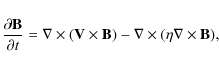
|
(1) |
where
As we are working in the framework of mean-field theory, we express both magnetic and velocity fields as a sum of large-scale (that will correspond to mean field) and small-scale (associated with fluid turbulence) contributions. Averaging over some suitably chosen intermediate scale makes it possible to write two distinct induction equations for the mean and the fluctuating parts of the magnetic field. A closure relation is then used to express the electromotive force in terms of mean magnetic field, leading to a simplified mean-field equation. In this work we will replace the emf by a surface Babcock-Leighton term (Babcock 1961; Leighton 1969; Wang et al. 1991; Dikpati & Charbonneau 1999; Jouve & Brun 2007a) as described in details below.
We work here in spherical
geometry and under the assumption of axisymmetry.
Reintroducing a poloidal/toroidal decomposition of the magnetic and
velocity fields in the mean induction equation, we get two coupled
partial differential equations, one involving the poloidal potential ![]() and the other concerning the toroidal field
and the other concerning the toroidal field ![]() .
.
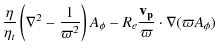
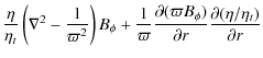
where
Equations (2) and (3) are solved in an annular meridional cut with the colatitude ![]()
![]() and the
radius (in dimensionless units)
and the
radius (in dimensionless units)
![]() i.e from slightly below the tachocline (r=0.7)
up to the solar surface, using the STELEM code.
This code has been thoroughly tested and validated thanks to an
international mean field dynamo benchmark involving 8 different codes
(Jouve et al. 2008). At
i.e from slightly below the tachocline (r=0.7)
up to the solar surface, using the STELEM code.
This code has been thoroughly tested and validated thanks to an
international mean field dynamo benchmark involving 8 different codes
(Jouve et al. 2008). At ![]() and
and
![]() boundaries, both
boundaries, both ![]() and
and ![]() are set to 0. Both
are set to 0. Both ![]() and
and ![]() are set to 0 at r=0.6. At the upper boundary, we smoothly match our solution to an external potential field, i.e. we have vacuum
for
are set to 0 at r=0.6. At the upper boundary, we smoothly match our solution to an external potential field, i.e. we have vacuum
for ![]() .
As initial conditions we are setting a confined dipolar field configuration, i.e the poloidal field is set to
.
As initial conditions we are setting a confined dipolar field configuration, i.e the poloidal field is set to
![]() in the convective zone and to 0 below the tachocline whereas the toroidal field is set to 0 everywhere.
in the convective zone and to 0 below the tachocline whereas the toroidal field is set to 0 everywhere.
3.2 The standard physical ingredients and the modified surface source term
We now need to prescribe the amplitude and profile of the various ingredients acting in Eqs. (2) and (3), namely the rotation, the diffusivity, the meridional flow and the Babcock-Leighton source term.
The rotation profile captures some realistic aspects of the Sun's
angular velocity, deduced from helioseismic inversions (Thompson
et al. 2003), assuming a solid rotation below 0.66 and a
differential rotation above the interface.
| |
= | ![$\displaystyle \Omega_{\rm c}+\frac{1}{2}\left[1+\rm erf(2\frac{r-r_{\rm c}}{{\rm d}_{1}})\right]$](/articles/aa/full_html/2010/11/aa14455-10/img53.png)
|
|
| (4) |
with
We assume that the diffusivity in the envelope ![]() is dominated by its turbulent contribution whereas in the stable interior
is dominated by its turbulent contribution whereas in the stable interior
![]() .
We smoothly match the two different constant values with an error function which enables us to
quickly and continuously transit from
.
We smoothly match the two different constant values with an error function which enables us to
quickly and continuously transit from
![]() to
to
![]() i.e.
i.e.
![\begin{displaymath}\eta(r)=\eta_{\rm c}+\frac{1}{2}\left(\eta_{\rm t}-\eta_{\rm ...
...ht)\left[1+{\rm erf}\left(\frac{r-r_{\rm c}}{d}\right)\right],
\end{displaymath}](/articles/aa/full_html/2010/11/aa14455-10/img62.png)
with
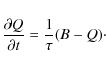
In Babcock-Leighton flux-transport dynamo models, meridional
circulation is used to link the two sources of the magnetic field
namely the base of the CZ and the solar surface.
For all the models presented in this paper we use a large single cell
per hemisphere, directed poleward at the surface, vanishing at the
bottom boundary r=0.6 and thus penetrating a little below the tachocline.
We take a stream function
which gives, through the relation
| ur | = | 
|
(7) |
|
|
= | ![$\displaystyle \Bigg[\frac{3r-r_{\rm b}}{1-r_{\rm b}} \sin\left(\pi\frac{r-r_{\r...
...m b})}{(1-r_{\rm b})} \cos\left(\pi\frac{r-r_{\rm b}}{1-r_{\rm b}}\right)\Bigg]$](/articles/aa/full_html/2010/11/aa14455-10/img68.png)
|
|
| (8) |
with
In Babcock-Leighton dynamo models, the poloidal field owes its origin to the tilt of magnetic loops emerging at the solar surface. Since these emerging loops are thought to rise from the base of the convection zone through magnetic buoyancy, we see that we can directly relate the way we model the Babcock-Leighton (BL) source term and the results of 3D calculations shown in Sect. 2.
In the standard model, the source term is confined in a thin layer at the surface and is made to be antisymmetric with respect to the equator, due to the sign of the Coriolis force which changes from one hemisphere to the other. These features are retained in our modified version.
However, the standard term is proportional to the toroidal field at the base of the convection zone at the same time, implying an instantaneous rise of the flux tubes from the base to the surface where they create tilted active regions. The 3D calculations showed that the rise velocity and thus the rise time depend on the field strength at the base of the CZ, we thus introduce in our modified version of the source term, a magnetic field-dependent time delay in the toroidal field at the base of the convection zone. We thus take into account the time delay between the formation of strong toroidal structures at the base of the convection zone and the surface regeneration of poloidal field.
The modified expression of the source term is thus
![$\displaystyle \frac{1}{2}\Bigg[1+\rm erf\left(\frac{r-r_{2}}{{\rm d}_{2}}\right)\Bigg]\Bigg[ 1-erf\left(\frac{r-1}{{\rm d}_{2}}\right)\Bigg]$](/articles/aa/full_html/2010/11/aa14455-10/img72.png)
![$\displaystyle \times ~ \Bigg[1+\left({\frac{B_{\phi}\left(r_{\rm c},\theta,t-\tau_B\right)}{B_{0}}}\right)^{2}\Bigg]^{-1}$](/articles/aa/full_html/2010/11/aa14455-10/img73.png)
where r2=0.95, d2=0.01,
In our 3D simulations, the approximate rise time for a
Finally, we take into account the fact that very strong toroidal
structures (more than
![]() )
are not influenced by the
Coriolis force enough to gain a significant tilt as they reach the
surface. To do so, we introduce a quenching term in the surface source
which will make the regeneration of the poloidal field less effective
when the toroidal field at the base of the CZ is strong enough.
Inversely, when the flux tubes are too weak, they will not be able to
reach the surface at all, and will not take part into the regeneration
term for the poloidal field.
We thus prevent the weakest flux tubes (or equivalently the most
delayed ones) to take part in the regeneration of poloidal fields at
the surface. To do so, the source term is set to zero when the delays
are above a certain threshold value corresponding to a rise time of
approximately half a solar cycle.
)
are not influenced by the
Coriolis force enough to gain a significant tilt as they reach the
surface. To do so, we introduce a quenching term in the surface source
which will make the regeneration of the poloidal field less effective
when the toroidal field at the base of the CZ is strong enough.
Inversely, when the flux tubes are too weak, they will not be able to
reach the surface at all, and will not take part into the regeneration
term for the poloidal field.
We thus prevent the weakest flux tubes (or equivalently the most
delayed ones) to take part in the regeneration of poloidal fields at
the surface. To do so, the source term is set to zero when the delays
are above a certain threshold value corresponding to a rise time of
approximately half a solar cycle.
4 Results
4.1 The standard solution
We first quickly present the solutions of our dynamo equations for the standard case which has been extensively discussed and used in the community to model the solar cycle (e.g. Dikpati & Charbonneau 1999).
![\begin{figure}
\par\includegraphics[width=9cm]{14455fig3.ps}
\includegraphics[width=9cm]{14455fig4.ps}
\end{figure}](/articles/aa/full_html/2010/11/aa14455-10/img82.png)
|
Figure 2:
Time-latitude cut of the toroidal field at the base
of the convection zone (representing the butterfly diagram)
and temporal evolution of the toroidal field energy
|
| Open with DEXTER | |
Figure 2 shows the typical solution of a
Babcock-Leighton standard dynamo model with a realistic choice of
parameters. This is the same case as the reference case of Jouve & Brun (2007a). In particular, the maximum latitudinal velocity at the
base of the convection zone (which is the significant velocity for the
advection of strong toroidal fields close to the tachocline) is set to
about
![]() .
.
The butterfly diagram resulting from this particular model is in good agreement with the observed migration of sunspots at the surface. In particular, a strong equatorward branch stretching from the mid-latitudes to the equator is clearly visible on the upper panel of Fig. 2. A strong poleward branch also appears in the evolution of the toroidal field at the interface, which is quite typical of Babcock-Leighton models. Indeed, it is the result of the combined action of low diffusivity at the base of the convection zone and strong radial shear linked to the differential rotation profile. It has been shown that both higher diffusivities (Dikpati & Charbonneau 1999) and penetration of the meridional flow below the core-envelope interface (Nandy & Choudhuri 2002) could prevent such a branch to appear. However, since our goal is more to study the effects of time delays in BL models than to build a calibrated solar-like solution, we adopt this solution as our reference case.
Nevertheless, it has here to be pointed out that making the link between the evolution of toroidal field at the base of the convection zone and the sunspots location at the solar surface during a magnetic cycle is not straightforward. Indeed, to be able to make this link, we have to assume that the rise of toroidal structures from the base of the convection zone to the surface is radial. However, as Choudhuri & Gilman (1987) first demonstrated using the thin flux tube approximation and as Fan (2008) confirmed with 3D MHD simulations, initially weak magnetic flux tubes are deviated from the radial trajectory and tend to follow a path which is parallel to the rotation axis while they make their way to the solar surface. In the simulations presented here, we do not take into account this drift in latitude of weak structures but intend to do so in a future work. We thus assume the evolution of toroidal field at the base of the convection zone to be a good proxy for the sunspot migration at the surface but keep in mind that the butterfly diagram may take a different form if the latitudinal drift is taken into account.
The lower panel of Fig. 2 shows the time evolution of
the toroidal field energy at the base of the convection zone and at
the latitude of
![]() ,
inside the activity belt. We clearly note that for the choice of
parameters we made, the solution is harmonic in time, no modulation of
the cycle is visible. As pointed out in the introduction,
Charbonneau et al. (2005) showed that a variation of the strength of the
Babcock-Leighton poloidal source term could lead to a chaotic behaviour
of the solutions through a sequence of bifurcations. In order to focus
on the influence of the time delays on the modulation of the
cycle, we chose
here a value of Cs which lies in the range of values for which no
modulation of the cycle can arise for the standard solution.
,
inside the activity belt. We clearly note that for the choice of
parameters we made, the solution is harmonic in time, no modulation of
the cycle is visible. As pointed out in the introduction,
Charbonneau et al. (2005) showed that a variation of the strength of the
Babcock-Leighton poloidal source term could lead to a chaotic behaviour
of the solutions through a sequence of bifurcations. In order to focus
on the influence of the time delays on the modulation of the
cycle, we chose
here a value of Cs which lies in the range of values for which no
modulation of the cycle can arise for the standard solution.
![\begin{figure}
\par\includegraphics[width=9.cm]{14455fig5.ps}
\includegraphics[width=9.cm]{14455fig6.ps}
\end{figure}](/articles/aa/full_html/2010/11/aa14455-10/img85.png)
|
Figure 3:
Same as Fig. 2 but with a delay of 14 days on 1 |
| Open with DEXTER | |
4.2 Introducing moderate delays
We now turn to investigate the effect of introducing a magnetic field-dependent delay in the model, modifying the surface source term according to Eq. (9). In particular, we focus on the modification of the butterfly diagram and the evolution of the toroidal field energy at a particular point in space.
Figure 3 shows the butterfly diagram and toroidal field
energy for a few cycles in the case where a small delay is
introduced. More precisely, a delay of 14 days is imposed on 1 ![]() fields at the base of the convection zone. According to the
dependence of the delay on the magnetic field intensity, it means that
10
fields at the base of the convection zone. According to the
dependence of the delay on the magnetic field intensity, it means that
10 ![]() fields will only be delayed by less than 4 hours, which is
extremely small compared to the time scale of the magnetic cycle.
However, even if the effects are hardly visible on the butterfly
diagram (it is almost indistinguishable from the one of
Fig. 2), a clear modulation of the magnetic energy
appears on the lower panel of Fig. 3.
The small
modification of the butterfly diagram is not surprising considering
the fact that the same physical processes still act in our model to
generate and advect the 3 components of the magnetic field. In
particular, the meridional flow, responsible for the advection of
toroidal fields at
the base of the convection zone, still acts to produce the
characteristic equatorward
branch of sunspot migration. What is more striking is the effect on
the cycle amplitude which becomes modulated, while the cycle period
remains approximately constant and identical to the standard case. To
understand this
particular feature, we will proceed to the study of a reduced model in
the following section. But first, the effects of higher delays are
analysed.
fields will only be delayed by less than 4 hours, which is
extremely small compared to the time scale of the magnetic cycle.
However, even if the effects are hardly visible on the butterfly
diagram (it is almost indistinguishable from the one of
Fig. 2), a clear modulation of the magnetic energy
appears on the lower panel of Fig. 3.
The small
modification of the butterfly diagram is not surprising considering
the fact that the same physical processes still act in our model to
generate and advect the 3 components of the magnetic field. In
particular, the meridional flow, responsible for the advection of
toroidal fields at
the base of the convection zone, still acts to produce the
characteristic equatorward
branch of sunspot migration. What is more striking is the effect on
the cycle amplitude which becomes modulated, while the cycle period
remains approximately constant and identical to the standard case. To
understand this
particular feature, we will proceed to the study of a reduced model in
the following section. But first, the effects of higher delays are
analysed.
4.3 Strong delays leading to highly perturbed solutions
The time delay is now increased from 14 days on 1 ![]() fields to 14 days on 50
fields to 14 days on 50 ![]() fields, meaning that 10
fields, meaning that 10 ![]() fields will be delayed by almost a year in this case (compared to a
few hours in the previous calculation). We point out again that the
maximum delay which can be reached for very weak tubes is about 6
years (approximately half a cycle), since a longer time for toroidal
structures to cross the convection zone would be unrealistic.
fields will be delayed by almost a year in this case (compared to a
few hours in the previous calculation). We point out again that the
maximum delay which can be reached for very weak tubes is about 6
years (approximately half a cycle), since a longer time for toroidal
structures to cross the convection zone would be unrealistic.
Figure 4 shows the butterfly diagram and the evolution of the magnetic energy for this case. This case is particularly interesting when we turn to consider the evolution of the toroidal energy with time. Indeed, again the effects on the shape of the butterfly diagram stay weak, even if some perturbations are clearly visible. In particular, close to the equator, consecutive cycles of the same polarity seem to connect, leading the cycle period at these latitudes to be different from the basic 11-yr cycle still present at higher latitudes. We also note that the period varies from one cycle to another but this particular feature is even more visible on the lower panel of Fig. 4.
![\begin{figure}
\par\includegraphics[width=9cm]{14455fig7.ps}
\includegraphics[width=9cm]{14455fig8.ps}
\end{figure}](/articles/aa/full_html/2010/11/aa14455-10/img86.png)
|
Figure 4:
Same as Fig. 2 but with a delay of 14 days on 50 |
| Open with DEXTER | |
The major effect of the delays is again to modulate the amplitude of the cycle to such a point that the weakest cycle on the particular period shown in Fig. 4 reaches in terms of peak energy only 30% of the peak energy of the strongest cycle. These variations are comparable to the observations of the monthly sunspot number available from 1750 until today (e.g. Hoyt & Schatten 1998). Indeed, over this period of time, the weakest cycle (cycle 5, which reached its peak in 1804) has been shown to possess a sunspot number of about 50 whereas the strongest cycle (cycle 19, which reached its maximum value in 1955) reached a sunspot number of more than 200. These strong variations are thus reproduced in this model with rather strong delays, but still small compared to the cycle period.
Finally, we should stress the variety of morphologies exhibited by the different cycles. In particular, some cycles show a clear asymmetry between their rising and declining phases (for example the cycle peaking at t = 895). Interestingly, we also note that some cycles seem to possess almost two peaks (as was observed on cycle 23) or at least show a change of slope in the declining phase, which makes them quite different from the standard more ``classical'' cycle.
To better understand the results of such a modulation in the amplitude and possibly on the period of the modelled solar cycle, we need to get back to a reduced model and analyse its properties from a dynamical systems point of view.
5 Understanding the modulation: reduction to a 6th order system
5.1 Formulation and justification of the reduced model
The reduced model we decide to use does not explicitly contains
time-delays as in the 2D model. It rather introduces another variable
Q which will be delayed by time ![]() with respect to the toroidal field
B. Moreover, we now work in only one dimension in space.
The set of equations we thus want to solve here is the following:
with respect to the toroidal field
B. Moreover, we now work in only one dimension in space.
The set of equations we thus want to solve here is the following:
|
(10) |
|
(11) |
|
(12) |
This model is significantly simplified since the physical ingredients (the rotation rate, the magnetic diffusivity, the meridional flow and the source term) are taken to be constants.

We will nevertheless show that such a simple model with a varying time delay, even small, is able to reproduce a modulation in the cyclic behaviour of the solutions.
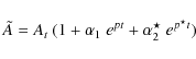
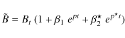
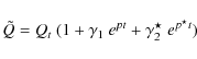
In order to simplify even more the previous set of equations, we take
the variables A, B and Q to be single Fourier modes in x,
with wavenumber k, such that:
we then get the following set of complex ODEs:
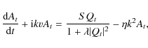
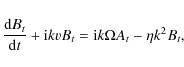
with
This choice of model was motivated by the fact that we want to study
this set of ODEs as a dynamical system. Having explicit delays in the equations
makes it much more difficult to identify the sequence of bifurcations
which could occur between the harmonic solution of
Fig. 2 and the aperiodic solution of
Fig. 4. Nevertheless, the new variable Qt introduced
in our simplified model and which now
represents the delayed toroidal field behaves exactly as we want it
to. To illustrate this, we solve the set of equations numerically for
the following choice of parameters:
![]() ,
S=100,
,
S=100,
![]() ,
v=10-2,
,
v=10-2,
![]() and
and
![]() where
where
![]() is a normalization factor. From now on, the values of
is a normalization factor. From now on, the values of ![]() will be expressed in terms of multiples of B12. We note
here that the actual time delays should not be directly related to the values of
will be expressed in terms of multiples of B12. We note
here that the actual time delays should not be directly related to the values of
![]() ,
because of this normalization factor.
,
because of this normalization factor.
These parameters are difficult to relate to the ones used in the full 2D model but they were chosen so that:
- dynamo action occurs (the dynamo number is high enough);
- the standard solution is harmonic in time (the dynamo number is low enough so it does not lead to any modulation of the cycle);
- we lie in the advection-dominated regime rather than in the
diffusion-dominated one (the advection time 1/k v is shorter than the
diffusive time
 ,
leading to
,
leading to  in our case where k=1);
- the time delay is always smaller than half a cycle period (i.e. we impose a maximum value for the time delay, like we did in the 2D model where the source was set to zero when the delay was too long).
![\begin{figure}
\par\includegraphics[width=8.cm]{14455fig9.ps} \end{figure}](/articles/aa/full_html/2010/11/aa14455-10/img104.png)
|
Figure 5: Temporal evolution of the toroidal field (plain line) and delayed toroidal field (dotted line) for a case where the delay is small enough to keep the harmonic solution stable. |
| Open with DEXTER | |
The second point which has to be noticed is the significantly lower
amplitude of ![]() compared to the original toroidal field
compared to the original toroidal field
![]() .
This amplitude difference is due to the fact that the
evolution equation for Qt is similar to a diffusion equation. This
property models the ohmic diffusion acting on the toroidal
flux tubes during their rise through the convection zone. Indeed, we
can reasonably expect the flux tubes reaching the surface to have a lower amplitude
than at the base of the convection zone. Moreover, the decrease in
strength will be higher when the initial magnetic field intensity in
the flux tubes is lower. Indeed, when the flux tubes are weaker, their
rise time is longer and becomes comparable to the diffusive time
associated to the magnetic structure, which is equal to
.
This amplitude difference is due to the fact that the
evolution equation for Qt is similar to a diffusion equation. This
property models the ohmic diffusion acting on the toroidal
flux tubes during their rise through the convection zone. Indeed, we
can reasonably expect the flux tubes reaching the surface to have a lower amplitude
than at the base of the convection zone. Moreover, the decrease in
strength will be higher when the initial magnetic field intensity in
the flux tubes is lower. Indeed, when the flux tubes are weaker, their
rise time is longer and becomes comparable to the diffusive time
associated to the magnetic structure, which is equal to ![]() when
the rising flux tube has a circular section of radius a. In our
reduced model, this effect is also taken into account since the
time delay for weaker tubes will be higher and thus the diffusion
operator will be more efficient in this case.
when
the rising flux tube has a circular section of radius a. In our
reduced model, this effect is also taken into account since the
time delay for weaker tubes will be higher and thus the diffusion
operator will be more efficient in this case.
With this choice of model and parameters, we are thus close to the dynamo solution calculated with the STELEM code presented in the previous section, so that we can reasonably relate the results of the reduced model to the full 2D calculations. The major interest of this type of models is that we are now reduced to a 6th order system which can be analysed both analytically and numerically.
5.2 Destabilization of the harmonic solution and influence of parameters
We now proceed to the analytic study of the characteristics of the harmonic solution when the delay is increased. In particular, we investigate the influence of the model parameters on the amplitude and frequency of the harmonic solution. The details of this analysis are presented in Appendix A.
As expected, the dynamo number
![]() controls the amplitude of our solution while the meridional
flow speed sets the cycle period. This behaviour is characteristic of
mean-field flux transport dynamo model and we are thus not going into
too many details. The effects of an increasing delay on both the
frequency and the amplitude of the solution is on the contrary of some
interest for our particular study.
controls the amplitude of our solution while the meridional
flow speed sets the cycle period. This behaviour is characteristic of
mean-field flux transport dynamo model and we are thus not going into
too many details. The effects of an increasing delay on both the
frequency and the amplitude of the solution is on the contrary of some
interest for our particular study.
| Figure 6:
Variation of the amplitude and the frequency of the
toroidal field Bt with the delay, for a particular
case. The choice of parameters is the same as in the
previous section, namely:
|
|
| Open with DEXTER | |
Figure 6 shows the variation of the amplitude and
frequency of the harmonic solution when the delay is increased when
all the other parameters are fixed to the values quoted in the
previous section. For higher values of the delay, the solution
becomes unstable, as we will see in the stability analysis below. The
standard ``undelayed'' solution is also included in these plots, for
![]() .
We note that the amplitude of our solution decreases
linearly with the delay which can be explained by the fact that the
amplitude of
.
We note that the amplitude of our solution decreases
linearly with the delay which can be explained by the fact that the
amplitude of ![]() (which represents the delayed toroidal field
and thus is the one responsible for the regeneration of the poloidal
field At) is smaller than the amplitude of Bt, due to the
diffusive effects included in our equations. Hence, the amount of
poloidal field generated by the reduced toroidal field will be weaker
and consequently, the toroidal field produced through the
(which represents the delayed toroidal field
and thus is the one responsible for the regeneration of the poloidal
field At) is smaller than the amplitude of Bt, due to the
diffusive effects included in our equations. Hence, the amount of
poloidal field generated by the reduced toroidal field will be weaker
and consequently, the toroidal field produced through the
![]() -effect acting on the poloidal field will also be reduced.
-effect acting on the poloidal field will also be reduced.
The frequency of the solution has a different behaviour when ![]() is
increased. Indeed, the variation is first close to linear with
is
increased. Indeed, the variation is first close to linear with ![]() ,
meaning that the cycle period is increased linearly with the delay but
then the slope of the curve changes and the cycle is significantly
slowed down by a variation of the delay. This feature can also be
understood by the fact that the regeneration of poloidal field will
take longer and longer when the delay is increased and thus the dynamo
loop will take longer to close.
,
meaning that the cycle period is increased linearly with the delay but
then the slope of the curve changes and the cycle is significantly
slowed down by a variation of the delay. This feature can also be
understood by the fact that the regeneration of poloidal field will
take longer and longer when the delay is increased and thus the dynamo
loop will take longer to close.
Another interesting point here is that we can study the effect of the various parameters on the threshold above which the harmonic solution becomes unstable. We will not focus on the effect of the dynamo number on this threshold since it has been studied in similar conditions before. Instead, we fix the dynamo number and we investigate the evolution of this threshold when the meridional flow speed is increased. The detailed stability analysis is shown in Appendix B. It has to be pointed out here that a Floquet analysis has been applied to our equations to investigate the nature of the bifurcation undergone by the system at that threshold. We find that two imaginary conjugate Floquet multipliers (reflecting the behaviour of a perturbation to the periodic solution after one cycle) cross the unit circle, thus indicating a Hopf bifurcation.
![\begin{figure}
\par\includegraphics[width=8.8cm]{14455fig12.ps}
\end{figure}](/articles/aa/full_html/2010/11/aa14455-10/img112.png)
|
Figure 7:
Value of |
| Open with DEXTER | |
Figure 7 shows the dependence of the critical
![]() (i.e. the value for which the harmonic solution becomes
unstable) with the meridional flow speed normalized by the magnetic
diffusivity. In our particular case where k=1 (and thus where
(i.e. the value for which the harmonic solution becomes
unstable) with the meridional flow speed normalized by the magnetic
diffusivity. In our particular case where k=1 (and thus where
![]() represents the ratio between diffusive and advective
times), this gives us some insight on the value of the delay
which has to be reached to get a modulation, when the system tends
more and more towards an advection dominated regime. The trend of the
threshold to decrease with increasing meridional flow speed is not
surprising if we consider we are introducing fixed values for the
delays, not normalized to the cycle period. Indeed, as v is
increased, the cycle period is decreased and then the absolute value
for the delay to have a significant effect on the cycle is
decreased. What is more striking is the saturation that the curve seems to
reach when v
is increased to strong values. In this case, the cycle
period (which is roughly inversely proportional to the meridional flow
speed in this type of models) is still decreased but the critical value
for the delay seems
to reach a minimum value. We thus conclude that the percentage of the
cycle represented by the critical delay will increase when the
meridional flow speed is increased. As an example, in the case where
the meridional
flow speed is quite weak (
represents the ratio between diffusive and advective
times), this gives us some insight on the value of the delay
which has to be reached to get a modulation, when the system tends
more and more towards an advection dominated regime. The trend of the
threshold to decrease with increasing meridional flow speed is not
surprising if we consider we are introducing fixed values for the
delays, not normalized to the cycle period. Indeed, as v is
increased, the cycle period is decreased and then the absolute value
for the delay to have a significant effect on the cycle is
decreased. What is more striking is the saturation that the curve seems to
reach when v
is increased to strong values. In this case, the cycle
period (which is roughly inversely proportional to the meridional flow
speed in this type of models) is still decreased but the critical value
for the delay seems
to reach a minimum value. We thus conclude that the percentage of the
cycle represented by the critical delay will increase when the
meridional flow speed is increased. As an example, in the case where
the meridional
flow speed is quite weak (![]() ), the threshold delay represents
about 14% of the cycle period whereas at
), the threshold delay represents
about 14% of the cycle period whereas at ![]() ,
this
percentage reaches
,
this
percentage reaches ![]() .
In this strongly advection-dominated
regime, the meridional flow speed is probably dominating the
time-scale of the system and as a result the effect of the delays is
reduced.
.
In this strongly advection-dominated
regime, the meridional flow speed is probably dominating the
time-scale of the system and as a result the effect of the delays is
reduced.
In the remainder of the paper, we focus on an intermediate case
(![]() ), where the threshold value for the delay
(
), where the threshold value for the delay
(
![]() )
reaches 19% of the cycle. This value
can appear quite large to the typical values for the delay used in the
full 2D model but it has to be pointed out that as soon as the
modulation appears, the strongest fields reach higher values than the
peak values of the harmonic solution. As a consequence, the delays for the strongest
fields are shorter and reach about 8% of the cycle, which is closer
to what was used in the 2D model.
This remark is related to the effect of fixed versus varying delays,
which we discuss in the conclusion.
)
reaches 19% of the cycle. This value
can appear quite large to the typical values for the delay used in the
full 2D model but it has to be pointed out that as soon as the
modulation appears, the strongest fields reach higher values than the
peak values of the harmonic solution. As a consequence, the delays for the strongest
fields are shorter and reach about 8% of the cycle, which is closer
to what was used in the 2D model.
This remark is related to the effect of fixed versus varying delays,
which we discuss in the conclusion.
5.3 Further evolution
Knowing the behaviour of the harmonic solution (which is stable for
small values of the delay) and the influence of the parameters,
we choose a particular set of those parameters to try to study a generic
solution when the delay is further increased. We thus choose numbers which
satisfy the conditions invoked in Sect. 5.1 and a
meridional flow speed in agreement with what was shown in the previous
section. The parameters chosen for all the analysis are the following:
![]() ,
S=100,
,
S=100,
![]() ,
v=10-2,
,
v=10-2,
![]() ,
the same as the ones
used for the solution shown in Fig. 6.
,
the same as the ones
used for the solution shown in Fig. 6.
![\begin{figure}
\par\includegraphics[width=8.5cm]{14455fig13.ps} \end{figure}](/articles/aa/full_html/2010/11/aa14455-10/img119.png)
|
Figure 8:
Time evolution of the toroidal magnetic energy with a
value of the delay of
|
| Open with DEXTER | |
Figure 8 shows the time series of the toroidal
magnetic energy for the solutions of the system when the delay is
further increased to
![]() .
An aperiodic modulation of the solar cycle
is here clearly visible, and the major point is that the evolution of
toroidal energy is very similar to what was found in the full 2D
system when the delay was sufficiently large (see
Fig. 4). Indeed, the major modulation acts on the cycle
amplitude but the frequency also varies and periods of very low
activity arise. This type of behaviour is very attractive when
compared to the observed sunspot number which qualitatively shows the
same kind of long-term variations. We should stress that we are still
here in a regime where the time delays are small compared to the
long-term modulation they seem to create. Moreover, this perturbed solution
is obtained both through 2D mean-field simulations and through a
reduced set of ODEs solving the Babcock-Leighton dynamo problem. These
results are
thus of particular interest as a new origin of modulation seems to
appear: the time delays due to the buoyant rise of flux tubes from the
base of the convection zone to the solar surface to create active
regions.
We now need to understand what happens to the system between the first
bifurcation and this aperiodic more interesting solution.
.
An aperiodic modulation of the solar cycle
is here clearly visible, and the major point is that the evolution of
toroidal energy is very similar to what was found in the full 2D
system when the delay was sufficiently large (see
Fig. 4). Indeed, the major modulation acts on the cycle
amplitude but the frequency also varies and periods of very low
activity arise. This type of behaviour is very attractive when
compared to the observed sunspot number which qualitatively shows the
same kind of long-term variations. We should stress that we are still
here in a regime where the time delays are small compared to the
long-term modulation they seem to create. Moreover, this perturbed solution
is obtained both through 2D mean-field simulations and through a
reduced set of ODEs solving the Babcock-Leighton dynamo problem. These
results are
thus of particular interest as a new origin of modulation seems to
appear: the time delays due to the buoyant rise of flux tubes from the
base of the convection zone to the solar surface to create active
regions.
We now need to understand what happens to the system between the first
bifurcation and this aperiodic more interesting solution.
We thus turn to investigate in more details which sequence of bifurcations leads to such complicated behaviour.
6 Beyond the first bifurcation: reduction to a 5th order system
To gain some insight on the behaviour of the system after the first bifurcation, we show that we can further reduce our problem from a 6th order to a 5th order system. Indeed, it is rather impractical to study the precise behaviour of the system after the first bifurcation. Reducing our system even more will help us achieve this goal.
6.1 Formulation of the model
Noticing that our system possesses a phase-invariance, i.e. a further symmetry, we follow the procedure of Weiss et al. (1984) and Jones et al. (1985) and make a change of variables which will remove this symmetry.
We express our variables At, Bt and Qt using polar
coordinates and introduce four new variables as shown


where y and z are complex numbers and
where

We then get a 5th order system since y and z are complex but
The interesting outcome of reducing our system from 6 degrees of freedom to 5 is that the limit cycle of the higher-order system now corresponds to a stationary solution in our reduced model and that a torus now corresponds to a limit cycle.
![\begin{figure}
\par\includegraphics[width=16.2cm,clip]{14455fig14.eps}
\end{figure}](/articles/aa/full_html/2010/11/aa14455-10/img131.png)
|
Figure 9:
Evolution of the system after
|
| Open with DEXTER | |
Solving this new system numerically will now enable us to analyze the further evolution of our solution when the delay is increased. In particular, we show that we can now easily exhibit the sequence of bifurcations leading to the aperiodic modulation of Fig. 8.
6.2 From the harmonic to the aperiodic solution: a sequence of bifurcations
We follow the evolution of our system from the first bifurcation
at
![]() to the aperiodic solution at
to the aperiodic solution at
![]() .
First, we can relate again these values to some physically
meaningful time-delays, keeping in mind that the system has been
simplified and that a particular choice of parameters was made. For
the stronger fields, a
value of
.
First, we can relate again these values to some physically
meaningful time-delays, keeping in mind that the system has been
simplified and that a particular choice of parameters was made. For
the stronger fields, a
value of
![]() would then correspond to a delay
of approximately a tenth of the cycle duration and
would then correspond to a delay
of approximately a tenth of the cycle duration and
![]() a third of the cycle period. These delays may
look higher than what was calculated in the 2D model but we showed
that a modification of the parameters (and especially of the
meridional flow speed) could move the threshold above which the
modulation starts to appear.
a third of the cycle period. These delays may
look higher than what was calculated in the 2D model but we showed
that a modification of the parameters (and especially of the
meridional flow speed) could move the threshold above which the
modulation starts to appear.
The Floquet
multipliers for this system are computed in order to study the stability of our periodic solution.
We find that the solution of our new reduced model
stays on a periodic orbit for a large range of values for the delay,
i.e. from
![]() to about
to about
![]() .
We
indeed find that at this value for the parameter
.
We
indeed find that at this value for the parameter ![]() ,
one of the
real Floquet multipliers crosses the unit circle through the -1 point,
indicating a period doubling bifurcation. This new 2-periodic solution then
persists for quite a large range of the control parameter until
we reach a new period doubling bifurcation.
,
one of the
real Floquet multipliers crosses the unit circle through the -1 point,
indicating a period doubling bifurcation. This new 2-periodic solution then
persists for quite a large range of the control parameter until
we reach a new period doubling bifurcation.
Figure 9 shows the evolution of the system from the
periodic solution resulting from the first Hopf bifurcation at
![]() until we reach the aperiodic modulations of
the cycle. We present on this figure a bifurcation diagram computed by
determining the maximum values of
until we reach the aperiodic modulations of
the cycle. We present on this figure a bifurcation diagram computed by
determining the maximum values of ![]() for each value of
for each value of
![]() (when the first period doubling has already
occurred). The initial branch existing at the beginning of the
bifurcation diagram thus indicates a periodic orbit. Moreover, phase portraits at key values of
the parameter are shown. They were chosen to stress the sequence of
period doubling bifurcations exhibited by the set of ODEs.
Panel b) shows the modification of the phase portrait of panel a) after the first period doubling has
occurred. We are then in the presence of a 2-periodic solution:
every 2 cycles, the value of
(when the first period doubling has already
occurred). The initial branch existing at the beginning of the
bifurcation diagram thus indicates a periodic orbit. Moreover, phase portraits at key values of
the parameter are shown. They were chosen to stress the sequence of
period doubling bifurcations exhibited by the set of ODEs.
Panel b) shows the modification of the phase portrait of panel a) after the first period doubling has
occurred. We are then in the presence of a 2-periodic solution:
every 2 cycles, the value of ![]() reaches the
same maximum value and this behaviour persists for as long as the model
has been calculated, i.e. for thousands of cycles. At
reaches the
same maximum value and this behaviour persists for as long as the model
has been calculated, i.e. for thousands of cycles. At
![]() ,
the system goes through another bifurcation. The
period is doubled again, which is visible both on the bifurcation
diagram (where the number of points is doubled at this value) and on
panel c). Indeed, the curve on the phase portrait closes on
itself after 4 cycles now instead of 2 for the previous values of
,
the system goes through another bifurcation. The
period is doubled again, which is visible both on the bifurcation
diagram (where the number of points is doubled at this value) and on
panel c). Indeed, the curve on the phase portrait closes on
itself after 4 cycles now instead of 2 for the previous values of
![]() .
Period doublings happen again at
.
Period doublings happen again at
![]() and
and
![]() where the solution becomes first 8-periodic and then
16-periodic. The phase portrait on panel d) shows the time
needed to close the curve is doubled at
where the solution becomes first 8-periodic and then
16-periodic. The phase portrait on panel d) shows the time
needed to close the curve is doubled at
![]() compared to the solution of panel c).
But
obviously, since the curve is
still closed, the system is still periodic.
compared to the solution of panel c).
But
obviously, since the curve is
still closed, the system is still periodic.
It then becomes difficult
to identify further period doublings but they may occur in very narrow
windows for the parameter. The main point is that the system seems to
reach a very complicated behaviour when the value of ![]() approaches
approaches
![]() .
Panel e) shows the phase portrait for
.
Panel e) shows the phase portrait for
![]() .
The phase space is almost entirely covered
by the solution and any value can be reached by the peaks in the
temporal evolution of
.
The phase space is almost entirely covered
by the solution and any value can be reached by the peaks in the
temporal evolution of ![]() ,
as shown on the bifurcation diagram. At this stage, a clear periodicity is
difficult to identify and we recover the strongly modulated solution
shown in Fig. 8 for a value of the parameter of
,
as shown on the bifurcation diagram. At this stage, a clear periodicity is
difficult to identify and we recover the strongly modulated solution
shown in Fig. 8 for a value of the parameter of
![]() .
.
Consequently, our system seems to undergo a sequence of period doublings leading to a chaotic behaviour. The solution may well be modified for higher values of the time-delays but which would not be realistic anymore for the physical process we are modelling. Similar cascades of period doublings have been found in the Lorenz equations (Sparrow 1982) and in other systems of ordinary and partial differential equations, including those governing the solar dynamo (Moore et al. 1983; Knobloch & Weiss 1983; Weiss et al. 1984; Knobloch et al. 1998). However, the nonlinearities at the origin of the sequence of bifurcations in those models were always related to the dynamical feedback of the Lorentz force on the flow. The striking result in this work is that modulation of the cycle amplitude can also arise in models where the only nonlinearities are the quenching term in the Babcock-Leighton source and the magnetic field-dependent time delays. It has here to be noted though that the time delays also appear in the quenching term (see Eq. (9)), possibly amplifying the nonlinear effects in the model.
We conclude that time delays due to flux tubes rising from the base of the convection zone to the surface seem to create a strongly modulated cycle in Babcock-Leighton dynamo models. A sequence of period doublings leading to chaos has clearly been identified here thanks to our 5th-order system. Indeed, even though it is also obviously present in the 6th order system, it is much more difficult to exhibit. The magnetic cycle resulting from these models which take into account the rise time of toroidal fields thus seems to be closer to the actual behaviour of the solar cycle.
7 Discussion and conclusion
In this work, we have introduced a more physically accurate model for the poloidal field source term in Babcock-Leighton flux transport dynamo models. To do so, some results from 3D MHD calculations of rising flux tubes from the base of the convection zone to the surface were reintroduced in 2D mean-field models. In particular, the rise time of flux ropes, which was assumed to be negligible in previous simulations, was here taken into account by introducing magnetic energy-dependent time delays in the BL source term. Through the use of a combination of analytical and numerical techniques applied to an adapted reduced system of non linear equations, we show that the system exhibits a sequence of bifurcations leading to a chaotic behaviour. The time evolution of the solution at that stage is qualitatively very similar to the full 2D model and more importantly to the actual solar activity, with strong modulation especially on the cycle amplitude.
Assuming the rise of flux tubes from the base of the convection zone
and the surface to be instantaneous and thus the time delays due to magnetic
buoyancy to be negligible can sound reasonable since these delays are
weak compared to the other time-scales of the system. In particular,
we can expect the time delay due to the advection by the meridional
flow (which has a characteristic time-scale of a few solar cycles, see
for example Charbonneau & Dikpati 2000) to
be much more effective on the behaviour of the dynamo-generated
magnetic field. As a consequence, it is mainly the effect of
meridional flow which has been tested in previous models (e.g. Wilmot-Smith et al. 2006). However, we showed here that the time delays due to
flux tubes rising have in fact a significant effect to modulate the
cycle on time scales very large compared to the delays. The main
reason for this behaviour is that the delays are not fixed but depend
on the modulated toroidal energy itself. To illustrate this
explanation, we show in Fig. 10 the time evolution of
toroidal fields (delayed and undelayed) for a case similar to what we showed in the core of the
paper (a
![]() -dependent delay with
-dependent delay with
![]() ,
i.e. just after the Hopf bifurcation) and the same evolution
when the delay is fixed to the mean value reached by the delay in the previous run.
,
i.e. just after the Hopf bifurcation) and the same evolution
when the delay is fixed to the mean value reached by the delay in the previous run.
![\begin{figure}
\par\includegraphics[width=8.5cm]{14455fig15.ps}
\includegraphics[width=8.5cm]{14455fig16.ps}
\end{figure}](/articles/aa/full_html/2010/11/aa14455-10/img144.png)
|
Figure 10:
Time evolution of the toroidal fields amplitude (undelayed in plain line and delayed in dotted line) for a
delay dependent on
|
| Open with DEXTER | |
On this figure, both the basic toroidal field and the delayed field are shown, stressing the time shift existing between the two. The striking result is that a long-term modulation appears only in the case of a varying delay. In the fixed-delay case, although the time-shift between the basic toroidal field and its delayed counterpart is quite significant compared to the cycle period, no modulation is created. On the contrary, in the varying-delay case, even though the strongest fields are almost not affected by the time-shift, a strong modulation on the amplitude is built up. As a result, the fact that small delays can affect the long-term evolution of the dynamo cycle seems to be linked to the variability of these delays and more specifically to their dependence on the magnetic field strength. Since magnetic buoyancy is much more efficient in the solar interior for strong toroidal field structures, these delays are likely to appear in reality. Consequently, a new origin of the solar cycle modulation may have been revealed here, thanks to the input of 3D MHD models into 2D mean-field dynamo calculations.
Only a part of the results of 3D calculations were reintroduced here but other effects can also be taken into account. In particular, hoop stresses and the Coriolis force are known since the first thin flux tubes simulations to deflect the trajectory of buoyantly rising magnetic fields inside the convection zone, this effect being stronger when the fields are less intense. This feature could also be introduced in BL models by modifying the source term for poloidal field. In particular, the source term is likely to get a contribution from the same latitude as the initial position of the flux tubes when those are strong enough and from a lower latitude when the flux tubes have been sufficiently influenced by the Coriolis force and the hoop stresses to rise parallel to the rotation axis. This may result in a different shape for the butterfly diagram with slightly more activity at higher latitudes, provided that weak magnetic structures are assumed to be able to reach the surface and create active regions. This could lead to reconsider the correspondence which is often made between toroidal magnetic field generated in 2D dynamo models at the base of the convection zone and the actual sunspot migration observed at the solar surface.
The variations of the solar cycle period are also known to be significant. For instance, cycle 23 has been significantly longer than the previous ones, with a duration of about 13 years (1996-2009). In the models computed in this work, the modulation of the solar activity is particularly visible on the cycle amplitude and is much less obvious on the period. However, the influence of rising flux tubes on the meridional flow was not taken into account here. Since the cycle period of the solutions resulting from these flux-transport models is very sensitive to the amplitude of the meridional circulation, a modification of the flow by rising flux tubes is very likely to modify the frequency of the dynamo solution and thus to also introduce a modulation on the cycle period. This feature is currently being investigated.
A considerable step forward would obviously be to develop a self-consistent global model with buoyant toroidal structures built up and making their way from the base of the convection zone where they become unstable to the photosphere where they create active regions. Unfortunately, this has not been achieved yet due to numerous physical and numerical difficulties. In the mean time, we have shown here that inputs from 3D MHD models simulating a particular step of the dynamo cycle can significantly improve 2D mean-field calculations. In particular, we have shown that they can even help reproducing a feature of the solar cycle (its variability) which was not present in the standard model before. We will continue to develop these ideas in future work.
AcknowledgementsL.J. and G.L. acknowledge support by STFC.
Appendix A: Amplitude and frequency of the harmonic solution
We can further expand our harmonic solution on a single Fourier mode in time as:
Reintroducing these expansions in Eqs. (13)-(15) will give us a way to calculate the frequency
Taking the real and imaginary parts of this relation dispersion give us the following equations
|
(A.2) |
|
(A.3) |
where
Appendix B: Stability of the harmonic solution
We can focus on the stability of this
periodic solution by perturbing it and studying the growth rates of
the perturbations. To do so, we perturb the solution as follows
|
(B.1) |
|
(B.2) |
|
(B.3) |
where
Substituting these expressions in Eqs. (13)-(15)
give us a system of 6 equations relating the coefficients of the
perturbations, the growth rate and all the parameters of the
system.
![\begin{displaymath}({\rm i}\omega+p+\eta+{\rm i}v)~ \alpha_1=({\rm i}\omega+\eta...
...t^2}{1+\lambda \vert Q_0 \vert ^2} ~(\gamma_1+\gamma_2)\right]
\end{displaymath}](/articles/aa/full_html/2010/11/aa14455-10/img165.png)
![\begin{displaymath}(-{\rm i}\omega+p+\eta-{\rm i}v)~\alpha_2\!=\!-({\rm i}\omega...
...{1\!+\!\lambda \vert Q_0 \vert ^2} ~(\gamma_1+\gamma_2)\right]
\end{displaymath}](/articles/aa/full_html/2010/11/aa14455-10/img166.png)
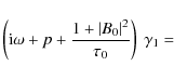
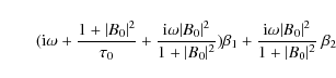
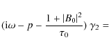
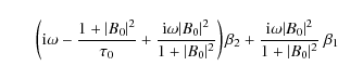

A non-trivial solution for this system exists only if the determinant is zero, we thus have to calculate the determinant and find the roots of the 6th order polynomial, in terms of the growth rate p. The harmonic solution loses stability at a Hopf bifurcation when the real part of one of the roots becomes positive.
References
- Archontis, V., Moreno-Insertis, F., Galsgaard, K., & Hood, A. W. 2005, ApJ, 635, 1299 [NASA ADS] [CrossRef] [Google Scholar]
- Babcock, H. W. 1961, ApJ, 133, 572 [Google Scholar]
- Bard, E., & Frank, M. 2006, Earth Planet. Sci. Lett., 248, 1 [NASA ADS] [CrossRef] [Google Scholar]
- Brun, A. S., Miesch, S. M., & Toomre, J. 2004, ApJ, 614, 1073 [NASA ADS] [CrossRef] [Google Scholar]
- Bushby, P. J. 2006, MNRAS, 371, 772 [Google Scholar]
- Caligari, P., Moreno-Insertis, F., & Schüssler, M. 1995, ApJ, 441, 886 [NASA ADS] [CrossRef] [Google Scholar]
- Cattaneo, F. 1999, ApJ, 515, L39 [NASA ADS] [CrossRef] [Google Scholar]
- Cattaneo, F., Brummell, N. H., & Cline, K. S. 2006, MNRAS, 365, 727 [NASA ADS] [CrossRef] [Google Scholar]
- Charbonneau, P. 2005, Liv. Rev. Sol. Phys., 2 [Google Scholar]
- Charbonneau, P., & Dikpati, M. 2000, ApJ, 543, 1027 [NASA ADS] [CrossRef] [Google Scholar]
- Charbonneau, P., St-Jean, C., & Zacharias, P. 2005, ApJ, 619, 613 [NASA ADS] [CrossRef] [Google Scholar]
- Cheung, M. C. M., Schüssler, M., & Moreno-Insertis, F. 2007, A&A, 467, 703 [NASA ADS] [CrossRef] [EDP Sciences] [Google Scholar]
- Choudhuri, A., & Gilman, P. 1987, ApJ, 316, 788 [NASA ADS] [CrossRef] [Google Scholar]
- Cline, K. S. 2003, Ph.D. Thesis [Google Scholar]
- Clune, T. L., Elliott, J. R., Glatzmaier, G. A., Miesch, M. S., & Toomre, J. 1999, Parallel Comput., 25, 361 [CrossRef] [Google Scholar]
- D'Silva, S., & Choudhuri, A. R. 1993, A&A, 272, 621 [NASA ADS] [Google Scholar]
- Dikpati, M., & Charbonneau, P. 1999, ApJ, 518, 508 [NASA ADS] [CrossRef] [Google Scholar]
- Dikpati, M., & Gilman, P. A. 2006, ApJ, 649, 498 [NASA ADS] [CrossRef] [Google Scholar]
- Dorch, S. B. F., Gudiksen, B. V., Abbett, W. P., & Nordlund, Å 2001, A&A, 380, 734 [NASA ADS] [CrossRef] [EDP Sciences] [Google Scholar]
- Durney, B. R. 1995, Sol. Phys., 160, 213 [Google Scholar]
- Eddy, J. A. 1976, Science, 192, 1189 [NASA ADS] [CrossRef] [PubMed] [Google Scholar]
- Fan, Y. 2004, Liv. Rev. Sol. Phys., 1, 1 [Google Scholar]
- Fan, Y. 2008, ApJ, 676, 680 [NASA ADS] [CrossRef] [Google Scholar]
- Fan, Y., Fisher, G. H., & McClymont, A. N. 1994, ApJ, 436, 907 [NASA ADS] [CrossRef] [Google Scholar]
- Fan, Y., Abbett, W. P., & Fisher, G. H. 2003, ApJ, 582, 1206 [NASA ADS] [CrossRef] [Google Scholar]
- Gilman, P. A. 1983, ApJs, 53, 243 [Google Scholar]
- Glatzmaier, G. A. 1987, The Internal Solar Angular Velocity, ed. B. R. Durney, & S. Sofia (Dordrecht: D. Reidel), 263 [Google Scholar]
- Hoyng, P. 1988, ApJ, 332, 857 [NASA ADS] [CrossRef] [Google Scholar]
- Hoyt, D. V., & Schatten, K. H. 1998, Sol. Phys., 181, 491 [NASA ADS] [CrossRef] [Google Scholar]
- Jones, C. A., Weiss, N. O., & Cattaneo, F. 1985, Phys. D Nonlinear Phenomena, 14, 161 [Google Scholar]
- Jouve, L., & Brun, A. S. 2007, A&A, 474, 239 [NASA ADS] [CrossRef] [EDP Sciences] [Google Scholar]
- Jouve, L., Brun, A. S., Arlt, R., et al. 2008, A&A, 483, 949 [NASA ADS] [CrossRef] [EDP Sciences] [Google Scholar]
- Jouve, L., Brun, A. S., Arlt, R., et al. 2009, ApJ, 701, 1300 [NASA ADS] [CrossRef] [Google Scholar]
- Knobloch, E., & Weiss, N. O. 1983, Phys. D Nonlinear Phenomena, 9, 379 [NASA ADS] [CrossRef] [Google Scholar]
- Knobloch, E., Tobias, S. M., & Weiss, N. O. 1998, MNRAS, 297, 1123 [Google Scholar]
- Krause, F., & Rädler, K. H. 1980, Mean Field Magnetohydrodynamics and Dynamo Theory, (Oxford: Pergamon Press) [Google Scholar]
- Lean, J. 2005, Physics Today, 58, 060000 [CrossRef] [Google Scholar]
- Leighton, R. B. 1969, ApJ, 156, 1 [Google Scholar]
- Magara, T. 2004, ApJ, 605, 480 [NASA ADS] [CrossRef] [Google Scholar]
- Martínez-Sykora, J., Hansteen, V., & Carlsson, M. 2008, ApJ, 679, 871 [NASA ADS] [CrossRef] [Google Scholar]
- Miesch, M. S. 2005, Liv. Rev. Sol. Phys., 2, 1 [Google Scholar]
- Miesch, M. S., Elliott, J. R., Toomre, J., et al. 2000, ApJ, 532, 593 [NASA ADS] [CrossRef] [Google Scholar]
- Moore, D. R., Toomre, J., Knobloch, E., & Weiss, N. O. 1983, Nature, 303, 663 [NASA ADS] [CrossRef] [Google Scholar]
- Moss, D., & Brooke, J. 2000, MNRAS, 315, 521 [NASA ADS] [CrossRef] [Google Scholar]
- Nandy, D., & Choudhuri, A. R. 2001, ApJ, 551, 576 [NASA ADS] [CrossRef] [Google Scholar]
- Nandy, D., & Choudhuri, A. R. 2002, Science, 296, 1671 [NASA ADS] [CrossRef] [PubMed] [Google Scholar]
- Ossendrijver, A. J. H., & Hoyng, P. 1996, A&A, 313, 959 [NASA ADS] [Google Scholar]
- Parker, E. N. 1955, ApJ, 121, 491 [NASA ADS] [CrossRef] [Google Scholar]
- Proctor, M. R. E. 1977, J. Fluid Mech., 80, 769 [NASA ADS] [CrossRef] [Google Scholar]
- Roberts, P. H. 1972, Phil. Trans. R. Soc. London, 272, 663 [Google Scholar]
- Rempel, M. 2006, ApJ, 647, 662 [NASA ADS] [CrossRef] [Google Scholar]
- Sparrow, C. T. 1982, The Lorenz equations: Bifurcations, Chaos and Strange Attractors (Berlin: Springer) [Google Scholar]
- Steenbeck, M., & Krause, F. 1969, Astron. Nachr., 291, 49 [NASA ADS] [CrossRef] [Google Scholar]
- Stix, M. 1976, A&A, 47, 243 [NASA ADS] [Google Scholar]
- Weiss, N. O., & Tobias, S. M. 2000, Space Sci. Rev., 94, 99 [NASA ADS] [CrossRef] [Google Scholar]
- Tobias, S. M. 1997, A&A, 322, 1007 [NASA ADS] [Google Scholar]
- Wang, Y.-M., Sheeley, N. R., Jr., & Nash, A. G. 1991, ApJ, 383, 431 [NASA ADS] [CrossRef] [Google Scholar]
- Weiss, N. O., Cattaneo, F., & Jones, C. A. 1984, Geophys. Astrophys. Fluid Dyn., 30, 305 [Google Scholar]
- Wilmot-Smith, A. L., Nandy, D., Hornig, G., & Martens, P. C. H. 2006, ApJ, 652, 696 [NASA ADS] [CrossRef] [Google Scholar]
- Yoshimura, H. 1978, ApJ, 226, 706 [NASA ADS] [CrossRef] [Google Scholar]
All Figures
|
|
Figure 1:
Rise velocity of tubes
introduced at 5
|
| Open with DEXTER | |
| In the text | |
|
|
Figure 2:
Time-latitude cut of the toroidal field at the base
of the convection zone (representing the butterfly diagram)
and temporal evolution of the toroidal field energy
|
| Open with DEXTER | |
| In the text | |
|
|
Figure 3:
Same as Fig. 2 but with a delay of 14 days on 1 |
| Open with DEXTER | |
| In the text | |
|
|
Figure 4:
Same as Fig. 2 but with a delay of 14 days on 50 |
| Open with DEXTER | |
| In the text | |
|
|
Figure 5: Temporal evolution of the toroidal field (plain line) and delayed toroidal field (dotted line) for a case where the delay is small enough to keep the harmonic solution stable. |
| Open with DEXTER | |
| In the text | |
| |
Figure 6:
Variation of the amplitude and the frequency of the
toroidal field Bt with the delay, for a particular
case. The choice of parameters is the same as in the
previous section, namely:
|
| Open with DEXTER | |
| In the text | |
|
|
Figure 7:
Value of |
| Open with DEXTER | |
| In the text | |
|
|
Figure 8:
Time evolution of the toroidal magnetic energy with a
value of the delay of
|
| Open with DEXTER | |
| In the text | |
|
|
Figure 9:
Evolution of the system after
|
| Open with DEXTER | |
| In the text | |
|
|
Figure 10:
Time evolution of the toroidal fields amplitude (undelayed in plain line and delayed in dotted line) for a
delay dependent on
|
| Open with DEXTER | |
| In the text | |
Copyright ESO 2010
Current usage metrics show cumulative count of Article Views (full-text article views including HTML views, PDF and ePub downloads, according to the available data) and Abstracts Views on Vision4Press platform.
Data correspond to usage on the plateform after 2015. The current usage metrics is available 48-96 hours after online publication and is updated daily on week days.
Initial download of the metrics may take a while.