| Issue |
A&A
Volume 519, September 2010
|
|
|---|---|---|
| Article Number | A50 | |
| Number of page(s) | 9 | |
| Section | Stellar structure and evolution | |
| DOI | https://doi.org/10.1051/0004-6361/201014111 | |
| Published online | 10 September 2010 | |
Comoving frame models of hot star winds
I. Test of the Sobolev approximation in the case of pure line transitions
J. Krticka1 - J. Kubát2
1 - Ústav teoretické fyziky a astrofyziky PrF MU, 611 37 Brno, Czech
Republic
2 - Astronomický ústav, Akademie ved Ceské republiky, 251 65 Ondrejov,
Czech Republic
Received 21 January 2010 / Accepted 28 April 2010
Abstract
We provide hot star wind models with radiative force calculated using
the solution of comoving frame (CMF) radiative transfer equation. The
wind models are calculated for the first stars, O stars, and
the central stars of planetary nebulae. We show that without line
overlaps and with solely thermal line broadening the pure Sobolev
approximation provides a reliable estimate of the radiative force even
close to the wind sonic point. Consequently, models with the Sobolev
line force provide good approximations to solutions obtained with
non-Sobolev transfer. Taking line overlaps into account,
the radiative force becomes slightly lower, leading to a
decrease in the wind mass-loss rate by roughly 40%. Below the
sonic point, the CMF line force is significantly lower
than the Sobolev one. In the case of pure thermal broadening,
this does not influence the mass-loss rate, as the wind
mass-loss rate is set in the supersonic part of the wind. However, when
additional line broadening is present (e.g., the turbulent
one) the region of low CMF line force may extend outwards to the
regions where the mass-loss rate is set. This results in a
decrease in the wind mass-loss rate. This effect can at least partly
explain the low wind mass-loss rates derived from some observational
analyses of luminous O stars.
Key words: stars: winds, outflows - stars: mass-loss - stars: early-type - hydrodynamics - radiative transfer
1 Introduction
One of the most important galactic populations consists of massive stars, because these stars dominate the spectra of many galaxies and contribute significantly to the mass and momentum input into the interstellar matter. Moreover, massive stars end their active lives in gigantic explosions such as supernovae or even possibly as the progenitors of gamma-ray bursts (see Yoon & Langer 2005; Woosley & Heger 2006), producing huge amounts of heavier elements.
An important property of hot stars that significantly influences their final stages is the stellar wind (see, e.g., Puls et al. 2008b; Owocki 2004; Krticka & Kubát 2007a, for reviews dedicated to hot star winds). However, in stellar evolution calculations it is usually unnecessary to know detailed wind properties, but just the amount of mass expelled from the star per unit of time (mass-loss rate) as a function of stellar parameters (e.g., mass, effective temperature, radius, surface metallicity). However, for many hot stars we simply cannot estimate their true mass-loss rate with the precision necessary to calculate evolutionary models. The situation may be less problematic for luminous O stars, for which relatively good agreement between theoretical predictions and observational results seems to exist (Vink et al. 2001; Krticka & Kubát 2004; Pauldrach et al. 2001, hereafter nltei).
However, the agreement between theoretically predicted mass-loss rates and those derived from observations may be an illusion caused by the neglect of some physical effects in the wind, such as clumping (Bouret et al. 2003; Martins et al. 2005). As a result, the true mass-loss rates of O stars may be a few times lower than the standard wind theory predicts. This seems to be supported by the observations of Fullerton et al. (2006) of weak wind line profiles of P V. Last but not least, the unexpected occurrence of symmetrical X-ray line profiles seems to require relatively low wind mass-loss rates (Kramer et al. 2003).
Possibly unreliable estimates of hot star wind mass-loss rates are also problematic because altough more realistic evolutionary stellar models can be calculated, by including, e.g., rotation and magnetic fields, the wind mass-loss rates remain uncertain. Ideally, all observational indicators of mass-loss rate and theoretical models should find and predict similar mass-loss rates. From the observational point of view, more detailed models of line formation in inhomogeneous media may be necessary to obtain reliable line profiles, and consequently also estimate mass-loss rates (Oskinova et al. 2007; Sundqvist et al. 2010).
From the theoretical point of view, disagreement between theory and observations would imply that some of the assumptions used for the hot-star wind modeling are inaccurate. Part of the disagreement may be caused by using incorrect abundances (Krticka & Kubát 2007b), although the reason for a disagreement remains mainly unclear. A thorough inspection of all assumptions involved in the modeling is therefore strongly needed. As a first step in this direction, we studied the influence of X-rays on the wind structure of hot stars. It seems that X-rays alone cannot entirely explain the disagreement between theory and observations (Krticka & Kubát 2009) as their influence on wind mass-loss rates is small and they do not strongly affect the ionization fraction of many important ions, especially that of P V. On the other hand, the modified ionization equilibrium may affect the X-ray line formation (Krticka & Kubát 2009; Oskinova et al. 2006), and too ling cooling time in the post-shock region (Krticka & Kubát 2009; Cohen et al. 2008) may cause the so-called ``weak wind problem'' (Martins et al. 2004; Bouret et al. 2003; Marcolino et al. 2009).
One of the most important approximations in the hot-star wind modeling is the Sobolev approximation (Castor 1974; Sobolev 1947), which enables us to solve the line radiation transfer analytically. Some studies confirm its applicability in the supersonic part of smooth line-driven winds (Pauldrach et al. 1986; Hamann 1981; Puls 1987). However, the applicability of the Sobolev approximation is questionable especially in the regions close to the photosphere bacause of the existence of strong source function gradients (Owocki & Puls 1999). On the other hand, some models avoid using the Sobolev approximation and use only the comoving-frame (hereafter CMF) method of solving the radiative transfer equation (e.g., Gräfener & Hamann 2005).
We decided to test the applicability of the Sobolev approximation and include the CMF solution of the radiative transfer equation in our wind models. In this first paper of a series, we describe our method, and study the applicability of the Sobolev approximation using models neglecting continuum opacity.
2 Basic model assumptions
The models used in this paper are based on the NLTE wind models of Krticka & Kubát (2004, hereafter <)375#>nltei#. Here we summarise only their basic features and describe the inclusion of CMF line force.
We assume a spherically symmetric stationary stellar wind. The excitation and ionization state of the considered elements is derived from the statistical equilibrium (NLTE) equations. Ionic models are either adopted from the TLUSTY grid of model stellar atmospheres (Lanz & Hubeny 2007,2003) or are prepared by us using the data from the Opacity and Iron Projects (Nahar & Pradhan 1993; Chen & Pradhan 1999; Butler et al. 1993; Seaton et al. 1992; Zhang 1996; Nahar & Pradhan 1996; Luo & Pradhan 1989; Bautista 1996; Seaton 1987; Bautista & Pradhan 1997; Fernley et al. 1987; Sawey & Berrington 1992; Zhang & Pradhan 1997; Hummer et al. 1993). As in nltei, the solution of the radiative transfer equation for NLTE equations is artificially split into two parts, namely the radiative transfer in either the continuum or in lines. The solution to the radiative transfer equation in continuum is based on the Feautrier method in the spherical coordinates (Kubát 1993; Mihalas & Hummer 1974), and the line radiative transfer is solved in the Sobolev approximation (Castor 1974; Rybicki & Hummer 1978) neglecting continuum opacity and line overlaps.
In contrast to our previous models, the radiative transfer in
lines used for the calculation of the radiative force is solved in the
CMF (see Sect. 3)
neglecting the continuum opacity. The line radiative force is
calculated directly from the true chemical composition,
NLTE ionization and excitation balance, and CMF flux using
data from the VALD database (Piskunov et al. 1995; Kupka et al.
1999). We do not use the line-strength distribution function
parameterized by force multipliers k, ![]() ,
and
,
and ![]() .
.
The flux at the surface (used as the lower boundary condition for the radiative transfer in the wind) is taken from the H-He spherically symmetric NLTE model stellar atmospheres of Kubát (2003, and references therein).
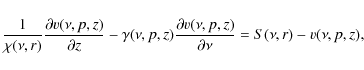
3 CMF calculation of the radiative force
The radiative force is calculated using the solution of the spherically symmetric CMF radiative transfer equation (Mihalas 1978, Eq. (14.99))
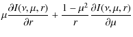
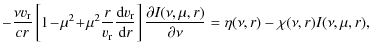
where
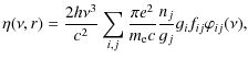
where ni
and nj
are the number densities of individual states with statistical
weights gi
and gj
corresponding to the line transition ![]() with oscillator strength fij
and the line-profile
with oscillator strength fij
and the line-profile
![]() ,
and
,
and ![]() is the electron mass. Assuming the line profile to be Gaussian produced
by thermal broadening only,
is the electron mass. Assuming the line profile to be Gaussian produced
by thermal broadening only, ![]() is
given by
is
given by
![\begin{displaymath}%
\varphi_{ij}(\nu)=\frac{1}{\sqrt\pi\Delta\nu_{ij}}
\exp\left[\frac{\left(\nu-\nu_{ij}\right)^2}{\Delta\nu_{ij}^2}\right],
\end{displaymath}](/articles/aa/full_html/2010/11/aa14111-10/img20.png)
|
(3) |
where
and
Writing Eq. (1), we neglected advection and aberration terms, which is justifiable in non-relativistic flows (see, e.g., Korcáková & Kubát 2003). We also note that by neglecting the spatial derivatives of intensity in Eq. (1) we obtain the Sobolev approximation (Castor 2004).
Following Mihalas
et al. (1975), we rewrite Eq. (1) for rays with an
impact parameter p
where + and - refers to radiation flowing toward and away from the observer, respectively, r=(p2+z2)1/2, and z is the distance along the ray. We transform Eq. (5) using intensity-like and flux-like variables
| (6a) | |||
| (6b) |
to obtain a system of partial differential equations
where
| (8) | |||
| (9) | |||
| (10) | |||
| (11) |
The system of equations in Eq. (7) is solved numerically using the long characteristic method of Mihalas et al. (1975), which we modified slightly for the present purpose (see Appendix A). As we are interested in the calculation of the radiative force using the v variable at a particular grid point, in contrast to Mihalas et al. (1975) we specify v at grid points, and u in the middle between them.
In our numerical solution of Eq. (7), we use the same
spatial grid as for the solution of hydrodynamical equations. The
spacing of the frequency grid is ![]() ,
where
,
where ![]() is
the pre-specified expected minimum wind temperature,
is
the pre-specified expected minimum wind temperature, ![]() is
the atomic mass of artificial metallic atom, and
is
the atomic mass of artificial metallic atom, and ![]() is
the multiplicative factor (see below). The CMF radiative
transfer equation is
solved only for selected frequencies from the frequency grid that lie
close to some line. The selection of frequencies is controlled by two
integer numbers
is
the multiplicative factor (see below). The CMF radiative
transfer equation is
solved only for selected frequencies from the frequency grid that lie
close to some line. The selection of frequencies is controlled by two
integer numbers ![]() ,
and NCERV (cf. Hillier & Miller
1998). For each line, we select frequencies that lie
within
,
and NCERV (cf. Hillier & Miller
1998). For each line, we select frequencies that lie
within ![]() line Doppler widths
line Doppler widths
![]() .
Redward of the center of each line, we select each NCERV frequency up
to the frequency corresponding to the Doppler shift for the wind
terminal velocity. The numerical test showed that a sufficiently
precise value of the radiative force can be derived for the value of
parameters
.
Redward of the center of each line, we select each NCERV frequency up
to the frequency corresponding to the Doppler shift for the wind
terminal velocity. The numerical test showed that a sufficiently
precise value of the radiative force can be derived for the value of
parameters ![]() ,
where
,
where ![]() is the mass of hydrogen atom,
is the mass of hydrogen atom, ![]() ,
,
![]() ,
NCERV = 30, and typically
,
NCERV = 30, and typically ![]() K.
K.
The radiative force is calculated as an integral
As the calculation of the CMF radiative force is rather time-consuming, we do not calculate

By the Sobolev line force
We note that direct use of Eq. (13) causes
instability in the model convergence. The reason for these convergence
problems may be numerical, but this behavior may also be connected with
line-driven instability (Feldmeier et al. 1997; Owocki et al.
1988). To avoid this (since we are seeking
stationary solution and not evolution with time) we introduced a weak
smoothing of
![]() ,
,
where
Table 1:
Radius R*, mass M,
and the effective temperature
![]() of studied model stars.
of studied model stars.
4 Studied model stars
In our study, we selected three types of stars to study more carefully the Sobolev approximation in different wind environments (see Table 1).
The stellar parameters of the first stars were obtained
according to an evolutionary calculation of initially zero-metallicity
star with initial mass ![]() derived by Marigo et al.
(2001). For these models, we assumed a stellar wind
driven purely by CNO elements (which appear on the stellar
surface
due to mixing) with a mass-fraction of CNO Z=10-3.
derived by Marigo et al.
(2001). For these models, we assumed a stellar wind
driven purely by CNO elements (which appear on the stellar
surface
due to mixing) with a mass-fraction of CNO Z=10-3.
The stellar parameters (effective temperatures and radii) of an O star sample were derived using the model atmospheres with line blanketing (Markova et al. 2004; Martins et al. 2005; Repolust et al. 2004). Stellar masses were obtained using evolutionary tracks either by ourselves (using Schaller et al. 1992 tracks) or by Martins et al. (2005). For these stars, we assumed a solar chemical composition (Asplund et al. 2005).
The stellar parameters of central stars of planetary nebulae were taken from Pauldrach et al. (2004), who derived them from UV spectroscopy. Helium abundance was adopted from Kudritzki et al. (1997), for other elements we assumed a solar chemical composition (after Asplund et al. 2005), which was for some stars slightly modified according to Pauldrach et al. (2004).
5 Comparison of CMF and Sobolev wind models
We calculated wind models with both CMF and Sobolev line forces and
compared the final wind structure. The resulting ratio of the CMF to
Sobolev line forces
![]() for selected stars is
shown in Fig. 1.
We note that the Sobolev force was calculated using the flux from the
stellar atmosphere and by neglecting line overlaps.
for selected stars is
shown in Fig. 1.
We note that the Sobolev force was calculated using the flux from the
stellar atmosphere and by neglecting line overlaps.
| Figure 1: The ratio of the CMF to Sobolev line forces given by Eq. (13) as a function of the wind velocity plotted in the terms of the sound speed for two selected stars. The dashed-dotted line denotes a model with constant source function and constant level populations equal to their values at the sonic point. Arrows indicate the thermal speed of selected ions. |
|
| Open with DEXTER | |
For very low wind velocities ![]() (where
(where ![]() ), the CMF
force is large,
), the CMF
force is large, ![]() .
This is most likely partly connected with the boundary conditions,
which are not completely compatible with the wind (cf., Noerdlinger & Rybicki 1974).
.
This is most likely partly connected with the boundary conditions,
which are not completely compatible with the wind (cf., Noerdlinger & Rybicki 1974).
For velocities of about one tenth of the sound speed, there is
an apparent minimum of
![]() .
In some cases, the ratio
.
In some cases, the ratio
![]() could even be negative, which corresponds to a negative CMF
radiative force. The Sobolev approximation is not applicable in this
region, but a low value of the radiative force is also connected with
positive source function gradients. For subsonic velocities,
the Doppler shift is less important, and the line radiative transfer is
given basically by the static radiative transfer equation. In the
optically thick regions, for frequencies corresponding to line
transitions it follows from Eq. (7b)
could even be negative, which corresponds to a negative CMF
radiative force. The Sobolev approximation is not applicable in this
region, but a low value of the radiative force is also connected with
positive source function gradients. For subsonic velocities,
the Doppler shift is less important, and the line radiative transfer is
given basically by the static radiative transfer equation. In the
optically thick regions, for frequencies corresponding to line
transitions it follows from Eq. (7b) ![]() ,
from Eq. (7a)
,
from Eq. (7a)
![]() ,
and the radiative force is proportional to the negative of the
derivative of the source function
,
and the radiative force is proportional to the negative of the
derivative of the source function ![]() (see Eq. (12),
and
Noerdlinger & Rybicki 1974).
Because the line source function increases here (see Fig. 2), the line
radiative force at low velocities may even be negative. For a constant
source function, the minimum of
(see Eq. (12),
and
Noerdlinger & Rybicki 1974).
Because the line source function increases here (see Fig. 2), the line
radiative force at low velocities may even be negative. For a constant
source function, the minimum of
![]() close to the star is significantly weaker (see Fig. 1). The source
function minimum below the sonic point is caused by a local temperature
minimum, because the line
source function of optically thick lines (which are, consequently, in
detailed radiative balance)
close to the star
close to the star is significantly weaker (see Fig. 1). The source
function minimum below the sonic point is caused by a local temperature
minimum, because the line
source function of optically thick lines (which are, consequently, in
detailed radiative balance)
close to the star ![]() (asterisk denotes LTE value) depends on temperature. Another
source function minimum for non-Sobolev source function due to velocity
field curvature was also found by Sellmaier
et al. (1993), and Owocki
& Puls (1999). We note that in the case of the
resonance lines plotted in Fig. 2 the line source
function at larger radii is roughly proportional to
(asterisk denotes LTE value) depends on temperature. Another
source function minimum for non-Sobolev source function due to velocity
field curvature was also found by Sellmaier
et al. (1993), and Owocki
& Puls (1999). We note that in the case of the
resonance lines plotted in Fig. 2 the line source
function at larger radii is roughly proportional to ![]() (e.g., Kudritzki & Puls 2000).
(e.g., Kudritzki & Puls 2000).
The minimum of ![]() close to the star is also connected with the velocity gradient changing
significantly within the resonance zone. Thus, a given line
also picks up the radiation corresponding to a lower velocity gradient
leading to a further reduction in the radiative force.
For velocities comparable to or higher than the ion thermal
speed, the lines are deshadowed because of the Doppler effect, and the
radiative force increases. We note that we only include the thermal
broadening, hence these effects occur for velocities lower than the
sound speed.
close to the star is also connected with the velocity gradient changing
significantly within the resonance zone. Thus, a given line
also picks up the radiation corresponding to a lower velocity gradient
leading to a further reduction in the radiative force.
For velocities comparable to or higher than the ion thermal
speed, the lines are deshadowed because of the Doppler effect, and the
radiative force increases. We note that we only include the thermal
broadening, hence these effects occur for velocities lower than the
sound speed.
| Figure 2:
The line source function for resonance lines of O IV
at 790 Å, S V
at 786 Å, and Fe V
at 388 Å as a function of relative wind velocity. The source
function is plotted relative to its value at the sonic point |
|
| Open with DEXTER | |
As the wind accelerates, the ratio of the CMF to Sobolev line force
increases and reaches a value
close to one for velocities higher than the thermal speed of the wind
driving ions (Fig. 1).
This is unsurprising, because the Sobolev approximation is applicable
to regions with a large velocity gradient, which exist already close to
the sonic point ![]() .
Owing to line overlaps,
.
Owing to line overlaps, ![]() is
less than one in the outer wind regions, where it reaches
only 0.7-0.8.
is
less than one in the outer wind regions, where it reaches
only 0.7-0.8.
| Figure 3: The radial variation in the ratio of the CMF to Sobolev line forces in the wind model of Tc 1 central star with and without line overlaps. |
|
| Open with DEXTER | |
To test the influence of line overlaps, we calculated the radiative
force with only 50 carefully selected optically thick lines
that do not overlap (see Fig. 3). The pronounced
minimum for velocities lower than the sound speed is still present
here, but in the outer regions the value of
![]() is approximately one, supporting the validity of the Sobolev
approximation for supersonic velocities.
is approximately one, supporting the validity of the Sobolev
approximation for supersonic velocities.
| Figure 4: The ratio of the CMF to Sobolev line forces at radius r=5 R*in the Tc1 wind model in the dependence on the line shift. The value of hydrogen thermal speed is denoted in the figure. |
|
| Open with DEXTER | |
To understand more clearly the influence of line overlaps on the
radiative force, we constructed
another artificial line list using our set of non-overlapping lines.
Each line in this new line list is counted twice with all parameters
being completely the same, however with a line center shifted by ![]() ,
where
,
where ![]() is a free parameter. For
is a free parameter. For
![]() ,
all twin lines completely overlap leading to a significant decrease in
the radiative force with respect to the Sobolev one that does not
account for the line overlaps (see Fig. 4). For
,
all twin lines completely overlap leading to a significant decrease in
the radiative force with respect to the Sobolev one that does not
account for the line overlaps (see Fig. 4). For
![]() ,
the lines at a given point do not overlap, but one of the twin lines
``sees'' the flux absorbed by the second line, leading to a reduction
in the radiative force even in this case. For
,
the lines at a given point do not overlap, but one of the twin lines
``sees'' the flux absorbed by the second line, leading to a reduction
in the radiative force even in this case. For
![]() ,
one of the lines is affected by the emission from the second one,
leading to an increase in the CMF radiative force relative to the
Sobolev one.
,
one of the lines is affected by the emission from the second one,
leading to an increase in the CMF radiative force relative to the
Sobolev one.
A similar reduction in the line force by multiline effects was found by Puls (1987). We note that the multiline effects were also studied with respect to the multiple radiative momentum deposition in Wolf-Rayet star winds (Gayley et al. 1995). However, these effects are probably of minor importance here due to the low density of the studied winds.
Table 2: Comparison of calculated wind parameters derived using CMF and Sobolev line forces.
The CMF radiative force, which is lower than the Sobolev one
because of line overlaps, causes a decrease in the mass-loss rate of
CMF models with respect to Sobolev ones (see Table 2). The ratio of CMF
to Sobolev mass-loss rates is about 0.58. The only exception
is the model M500-1, for which the CMF mass-loss rate is
nearly the same as the Sobolev one. The reason is that the star is so
hot, that the wind is accelerated mainly by a dozen O V
and O VI lines.
For a critical point velocity, these lines do not
overlap, hence ![]() ,
and the CMF and Sobolev mass-loss rates are nearly the same.
,
and the CMF and Sobolev mass-loss rates are nearly the same.
![\begin{figure}
\par\includegraphics[width=6.6cm,clip]{14111fg5.eps}\vspace*{2mm}
\includegraphics[width=6.6cm,clip]{14111fg6.eps}
\end{figure}](/articles/aa/full_html/2010/11/aa14111-10/img120.png)
|
Figure 5: Comparison of our derived mass-loss rates ( upper panel) and terminal velocities ( lower panel) of the central stars of planetary nebulae with those derived by Pauldrach et al. (2004). |
| Open with DEXTER | |
The resulting wind parameters of the central stars of planetary nebulae can be compared with those derived from observations by Pauldrach et al. (2004, see Fig. 5). There is reasonable agreement between the wind parameters predicted by ourselves and those derived by Pauldrach et al. (2004, see Fig. 5). The mass-loss rates of Pauldrach et al. (2004) are on average a factor of about 1.6 higher than those derived by ourselves. This is most likely partly because of the simplifications included in our code, e.g., the neglect of continuum opacity sources, and partly by the different abundances adopted.
6 Models with base turbulence
| Figure 6: The mass-loss rate of HD 209975 in the models with additional turbulent line broadening relative to the models with zero turbulent velocity. |
|
| Open with DEXTER | |
The existence of a region close to the stellar surface where the CMF line force is low compared to the Sobolev one (see Fig. 1) is partly caused by the source function gradients at the wind base and partly by the Sobolev approximation not being applicable to the subsonic regions. The CMF line force increases at the moment when the line starts to absorb the radiation that has not been absorbed yet, i.e., the radiation from the line wing. Because up to now we have assumed pure thermal line broadening, the velocity width of low CMF line force is of the order of the metallic thermal speed (which is roughly 0.13 a in the case of iron). The wind mass-loss rate in our models is determined in the region of supersonic wind, close to the critical point where the wind velocity approaches the speed of radiative-acoustic waves (Feldmeier et al. 2008; Abbott 1980). Thus, the region of low CMF line force close to the star does not significantly affect the wind mass-loss rate.
However, if the line broadening were larger (due to
surface turbulence), then the region of low
CMF line force could spread out to large velocities comparable
to the turbulent one. When the turbulent velocity is comparable to the
critical point velocity, below which the wind mass-loss rate
is set, this could cause a significant decrease in the wind mass-loss
rate. To test this, we calculated wind models with additional
line broadening, which we attributed to the turbulent one.
In this case, the line profile width is given not by
Eq. (4),
but by
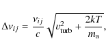
where
The results of numerical models indicate that with increasing turbulent broadening the velocity width of low CMF line force increases leading to a lower mass-loss rate (see Fig. 6, cf. Lucy 2007). Hence, in the presence of turbulence the wind parameters may not depend only on the basic stellar parameters (effective temperature, radius, mass) but also on the line turbulent broadening. Moreover, this effect can possibly be one of the reasons why the mass-loss rates derived from observational analyses that take the clumping into account (Bouret et al. 2003; Martins et al. 2005) are systematically lower than the predicted ones.
For velocities higher than a few times the turbulent one, the
Sobolev approximation should be applicable. At these high
velocities, one expects that the line force becomes close to the
Sobolev one. Because now the same force (as in the model with
zero turbulent broadening) accelerates the wind of lower density, one
expects the terminal velocity to increase (e.g., Gayley
2001),
becoming much higher than the observed one. However, our models do not
predict a significant increase in the terminal velocity ![]() ,
which is in the range
,
which is in the range ![]() for the
wind models of HD 209975 with different turbulent broadening.
This is caused by the stronger blocking of stellar radiation by
increased line overlaps mainly in the region with
for the
wind models of HD 209975 with different turbulent broadening.
This is caused by the stronger blocking of stellar radiation by
increased line overlaps mainly in the region with ![]() .
We note that lines broadened by turbulent motions are able to block the
flux more efficiently than
lines broadened purely thermally.
.
We note that lines broadened by turbulent motions are able to block the
flux more efficiently than
lines broadened purely thermally.
Observational studies consider the turbulence already present
in the photospheres of O stars (e.g., Bouret et al. 2005; Martins
et al. 2004; Bouret et al. 2003; Martins
et al. 2005) with turbulent velocities of about ![]() .
Macroturbulent velocities in B supergiants may be even higher,
about
.
Macroturbulent velocities in B supergiants may be even higher,
about ![]() (Markova
& Puls 2008; Howarth et al. 1997).
Convective layers and surface pulsational motions are also expected
theoretically (Cantiello et al.
2009; Aerts et al. 2009).
Turbulence can spread in the wind (Feldmeier
et al. 1997), leading to a decrease in the wind
mass-loss rate, as shown here. We also note that many
O stars exhibit turbulent velocities in the range
(Markova
& Puls 2008; Howarth et al. 1997).
Convective layers and surface pulsational motions are also expected
theoretically (Cantiello et al.
2009; Aerts et al. 2009).
Turbulence can spread in the wind (Feldmeier
et al. 1997), leading to a decrease in the wind
mass-loss rate, as shown here. We also note that many
O stars exhibit turbulent velocities in the range ![]() ,
where we expect a high sensitivity of the predicted mass-loss rate to
the turbulent velocity (see Fig. 6).
,
where we expect a high sensitivity of the predicted mass-loss rate to
the turbulent velocity (see Fig. 6).
The basic results presented here will, in the future, be tested in more detail using models that also account for the continuum opacity and CMF line source function in a separate study.
7 The solution topology
| Figure 7: The dependence of the radial velocity on radius for solutions with different boundary densities (mass-loss rates) close to the stellar surface for the model star 500-1. Each consecutive model (from down to up) differs by a factor of 1.5 in the mass-loss rate (thin lines). The thick line denotes the unique solution that smoothly intercepts the critical point. The dashed line denotes solution with the Sobolev line force. |
|
| Open with DEXTER | |
In Fig. 7, we plot solutions with different base densities (mass-loss rates). In generall, with increasing base density the wind velocity increases until the density reaches a maximum value. There is no solution that is smooth out to large radii for the densities higher than the maximum one. The solution with maximum density is very similar to the critical solution of Sobolev models (see Fig. 7). Moreover, there are many solutions that smoothly pass through the sonic point v=a for different mass-loss rates.
This indicates that the critical point of non-Sobolev models is close to the CAK critical point (Castor et al. 1975) and that the sonic point is not a point where the wind mass-loss rate is determined. The reason is that even in the non-Sobolev models the radiative force is not given locally by wind density and velocity, but depends on the wind properties in a close neighborhood of a studied point. This dependence on the non-local properties at its limit approaches the Sobolev approximation for very thin resonance layers (for very large velocity gradients).
8 Conclusions
We have presented hot star wind models in which the radiative force is calculated using the solution of the comoving frame (CMF) radiative transfer equation. The wind models were calculated for three different groups of stellar parameters (corresponding to evolved first stars, O stars, and the central stars of planetary nebulae) to compare the CMF and Sobolev radiative forces for a broader range of stellar parameters.
The comparison of the CMF radiative force with an approximate one calculated by assuming the Sobolev approximation showed that the Sobolev line force is slightly higher due to the neglect of line overlaps. Thus, the mass-loss rate of wind models that include the Sobolev line force is on average a factor of about 1.7 higher than a more realistic one calculated using CMF wind models. However, we note that the simple Sobolev approximation applied here for reference can be improved to account for line overlaps and continuum absorption (Olson 1982; Hummer & Rybicki 1985; Pavlakis & Kylafis 1996; Puls & Hummer 1988). We emphasize that modern hot star wind models include line overlaps (e.g., Vink et al. 2001; Gräfener & Hamann 2005; Pauldrach et al. 2001).
Without line overlaps in the case of purely thermal line broadening, the Sobolev approximation provides a reliable estimate of the radiative force even close to the wind sonic point. The CAK model therefore provides a good approximation for a solution obtained with non-Sobolev transfer. Below the sonic point, the CMF line force is significantly lower than the Sobolev one partly because of the strong gradients in the source function. This does not influence the mass-loss rate, as the wind mass-loss rate is set in the supersonic part of the wind below the critical point. However, when additional line broadening is present (e.g., the turbulent one) then the region of low CMF line force may extend outwards to the regions where the mass-loss rate is set. This results in a significant decrease in the wind mass-loss rate. We note that this is not a shortcoming of the Sobolev approximation because the Sobolev approximation is applicable to velocities higher than the turbulent velocity in this case.
The influence of turbulent line broadening may cause a dependence of the wind mass-loss rate on the atmospheric turbulent motions. Because theoretical models are not yet able to predict the atmospheric turbulent motions in hot stars in detail, we are unable to provide reliable wind mass-loss rate predictions until the theory of the atmospheric turbulence develops considerably (however see Aerts et al. 2009; Cantiello et al. 2009). Nowadays, hot star evolution seems to be a deterministic one depending only on the initial stellar parameters, i.e., mass, metallicity, and rotational rate. However, as the properties of atmospheric turbulent motions seem to be a non-trivial function of stellar parameters, the evolution of hot stars may become less deterministic, becoming instead dependent on free parameters describing the role of surface turbulence.
AcknowledgementsThis work was supported by grant GA CR 205/07/ 0031. The Astronomical Institute Ondrejov is supported by the project AV0 Z10030501.
References
- Abbott, D. C. 1980, ApJ, 242, 1183 [NASA ADS] [CrossRef] [Google Scholar]
- Aerts, C., Puls, J., Godart, M., & Dupret, M.-A. 2009, A&A, 508, 409 [NASA ADS] [CrossRef] [EDP Sciences] [Google Scholar]
- Anderson, E., Bai, Z., Bischof, C., et al. 1999, LAPACK Users' Guide, 3rd edn. (Philadelphia: SIAM) [Google Scholar]
- Asplund, M., Grevesse, N., & Sauval, A. J. 2005, in Cosmic Abundances as Records of Stellar Evolution and in Nucleosynthesis, ed. T. G. Barnes III, & F. N. Bash (San Francisco: ASP), ASP Conf. Ser., 336, 25 [Google Scholar]
- Bautista, M. A. 1996, A&AS, 119, 105 [Google Scholar]
- Bautista, M. A., & Pradhan, A. K. 1997, A&AS, 126, 365 [Google Scholar]
- Bouret, J.-C., Lanz, T., Hillier, D. J., et al. 2003, ApJ, 595, 1182 [NASA ADS] [CrossRef] [Google Scholar]
- Bouret, J.-C., Lanz, T., & Hillier, D. J. 2005, A&A, 438, 301 [NASA ADS] [CrossRef] [EDP Sciences] [Google Scholar]
- Butler, K., Mendoza, C., & Zeippen, C. J. 1993, J. Phys. B., 26, 4409 [NASA ADS] [CrossRef] [Google Scholar]
- Cantiello, M., Langer, N., Brott, I., et al. 2009, A&A, 499, 279 [NASA ADS] [CrossRef] [EDP Sciences] [Google Scholar]
- Castor, J. I. 1974, MNRAS, 169, 279 [NASA ADS] [CrossRef] [Google Scholar]
- Castor, J. I. 2004, Radiation Hydrodynamics (Cambridge: Cambridge University Press) [Google Scholar]
- Castor, J. I., Abbott, D. C., & Klein, R. I. 1975, ApJ, 195, 157 (CAK) [NASA ADS] [CrossRef] [Google Scholar]
- Chen, G. X., & Pradhan, A. K. 1999, A&AS, 136, 395 [Google Scholar]
- Cohen, D. H., Kuhn, M. A., Gagné, M., Jensen, E. L. N., & Miller, N. A. 2008, MNRAS, 386, 1855 [NASA ADS] [CrossRef] [Google Scholar]
- Feldmeier, A., Puls, J., & Pauldrach, A. W. A. 1997, A&A, 322, 878 [NASA ADS] [Google Scholar]
- Feldmeier, A., Rätzel, D., & Owocki, S. P. 2008, ApJ, 679, 704 [NASA ADS] [CrossRef] [Google Scholar]
- Fernley, J. A., Taylor, K. T., & Seaton, M. J. 1987, J. Phys. B, 20, 6457 [NASA ADS] [CrossRef] [Google Scholar]
- Fullerton, A. W., Massa, D. L., & Prinja, R. K. 2006, ApJ, 637, 1025 [NASA ADS] [CrossRef] [Google Scholar]
- Gayley, K. G. 2000, ApJ, 529, 1019 [NASA ADS] [CrossRef] [Google Scholar]
- Gayley, K. G., Owocki, S. P., & Cranmer, S. R. 1995, ApJ, 442, 296 [NASA ADS] [CrossRef] [Google Scholar]
- Gräfener, G., & Hamann, W.-R. 2005, A&A, 432, 633 [NASA ADS] [CrossRef] [EDP Sciences] [Google Scholar]
- Hamann, W.-R. 1981, A&A, 93, 353 [NASA ADS] [Google Scholar]
- Hillier, D. J., & Miller, D. L. 1998, ApJ, 496, 407 [NASA ADS] [CrossRef] [Google Scholar]
- Howarth, I. D., Siebert, K. W., Hussain, G. A. J., & Prinja, R. K. 1997, MNRAS, 284, 265 [NASA ADS] [CrossRef] [Google Scholar]
- Hummer, D. G., & Rybicki, G. B. 1985, ApJ, 293, 258 [NASA ADS] [CrossRef] [Google Scholar]
- Hummer, D. G., Berrington, K. A., Eissner, W., et al. 1993, A&A, 279, 298 [NASA ADS] [Google Scholar]
- Korcáková, D., & Kubát, J. 2003, A&A, 401, 419 [NASA ADS] [CrossRef] [EDP Sciences] [Google Scholar]
- Kramer, R. H., Cohen, D. H., & Owocki, S. P. 2003, ApJ, 592, 532 [NASA ADS] [CrossRef] [Google Scholar]
- Krticka, J., & Kubát, J. 2001, A&A, 369, 222 [NASA ADS] [CrossRef] [EDP Sciences] [Google Scholar]
- Krticka, J., & Kubát, J. 2004, A&A, 417, 1003 nltei [NASA ADS] [CrossRef] [EDP Sciences] [Google Scholar]
- Krticka, J., & Kubát, J. 2007a, in Active OB-Stars: Laboratories for Stellar & Circumstellar Physics, ed. S. Stefl, S. P. Owocki, & A. T. Okazaki (San Francisco: ASP), 153 [Google Scholar]
- Krticka, J., & Kubát, J. 2007b, A&A, 464, L17 [NASA ADS] [CrossRef] [EDP Sciences] [Google Scholar]
- Krticka, J., & Kubát, J. 2009, MNRAS, 394, 2065 [NASA ADS] [CrossRef] [Google Scholar]
- Kubát, J. 1993, Ph.D. Thesis, Astronomický ústav AV CR, Ondrejov [Google Scholar]
- Kubát, J. 2003, in Modelling of Stellar Atmospheres, ed. N. E. Piskunov, W. W. Weiss, & D. F. Gray (San Francisco: ASP), IAU Symp., 210, A8 [Google Scholar]
- Kudritzki, R. P., & Puls, J. 2000, ARA&A, 38, 613 [NASA ADS] [CrossRef] [Google Scholar]
- Kudritzki, R.-P., Méndez, R. H., Puls, J., & McCarthy, J. K. 1997, in Planetary Nebulae, ed. H. J. Habing, & H. J. G. L. M. Lamers, Proc. IAU Symp., 180, 64 [Google Scholar]
- Kupka, F., Piskunov, N. E., Ryabchikova, T. A., Stempels, H. C., & Weiss, W. W. 1999, A&AS, 138, 119 [NASA ADS] [CrossRef] [EDP Sciences] [MathSciNet] [PubMed] [Google Scholar]
- Lanz, T., & Hubeny, I. 2003, ApJS, 146, 417 [NASA ADS] [CrossRef] [Google Scholar]
- Lanz, T., & Hubeny, I. 2007, ApJS, 169, 83 [CrossRef] [Google Scholar]
- Lucy, L. B. 2007, A&A, 468, 649 [NASA ADS] [CrossRef] [EDP Sciences] [Google Scholar]
- Luo, D., & Pradhan, A. K. 1989, J. Phys. B, 22, 3377 [NASA ADS] [CrossRef] [Google Scholar]
- Marcolino, W. L. F., Bouret, J.-C., Martins, F., et al. 2009, A&A, 498, 837 [NASA ADS] [CrossRef] [EDP Sciences] [Google Scholar]
- Marigo, P., Girardi, L., Chiosi, C., & Wood, P. R. 2001, A&A, 371, 152 [NASA ADS] [CrossRef] [EDP Sciences] [Google Scholar]
- Markova, N., & Puls, J. 2008, A&A, 478, 823 [NASA ADS] [CrossRef] [EDP Sciences] [Google Scholar]
- Markova, N., Puls, J., Repolust, T., & Markov, H. 2004, A&A, 413, 693 [NASA ADS] [CrossRef] [EDP Sciences] [Google Scholar]
- Martins, F., Schaerer, D., Hillier, D. J., & Heydari-Malayeri, M. 2004, A&A, 420, 1087 [NASA ADS] [CrossRef] [EDP Sciences] [Google Scholar]
- Martins, F., Schaerer, D., Hillier, D. J., et al. 2005, A&A, 441, 735 [NASA ADS] [CrossRef] [EDP Sciences] [Google Scholar]
- Mihalas, D. 1978, Stellar Atmospheres (San Francisco: Freeman & Co.) [Google Scholar]
- Mihalas, D., & Hummer, D. G. 1974, ApJS, 28, 343 [NASA ADS] [CrossRef] [Google Scholar]
- Mihalas, D., Kunasz, P. B., & Hummer, D. G. 1975, ApJ, 202, 465 [NASA ADS] [CrossRef] [Google Scholar]
- Nahar, S. N., & Pradhan, A. K. 1993, J. Phys. B, 26, 1109 [NASA ADS] [CrossRef] [Google Scholar]
- Nahar, S. N., & Pradhan, A. K. 1996, A&AS, 119, 509 [Google Scholar]
- Noerdlinger, P. D., & Rybicki, G. B. 1974, ApJ, 193, 651 [NASA ADS] [CrossRef] [Google Scholar]
- Olson, G. L. 1982, ApJ, 255, 267 [NASA ADS] [CrossRef] [Google Scholar]
- Oskinova, L. M., Hamann, W.-R., & Feldmeier, A. 2006, in High Resolution X-ray Spectroscopy, ed. G. Branduardi-Raymont, 27 [Google Scholar]
- Oskinova, L. M., Hamann, W.-R., & Feldmeier, A. 2007, A&A, 476, 1331 [NASA ADS] [CrossRef] [EDP Sciences] [Google Scholar]
- Owocki, S. P. 2004, in Evolution of Massive Stars, Mass Loss and Winds, ed. M. Heydari-Malayeri, Ph. Stee, & J.-P. Zahn, EAS PS, 13, 163 [Google Scholar]
- Owocki, S. P., & Puls, J. 1999, ApJ, 510, 355 [NASA ADS] [CrossRef] [Google Scholar]
- Owocki, S. P., Castor, J. I., & Rybicki, G. B. 1988, ApJ, 335, 914 [NASA ADS] [CrossRef] [Google Scholar]
- Pauldrach, A., Puls, J., & Kudritzki, R. P. 1986, A&A, 164, 86 [NASA ADS] [Google Scholar]
- Pauldrach, A. W. A., Hoffmann, T. L., & Lennon, M. 2001, A&A, 375, 161 [NASA ADS] [CrossRef] [EDP Sciences] [Google Scholar]
- Pauldrach, A. W. A., Hoffmann, T. L., & Méndez, R. H. 2004, A&A, 419, 1111 [NASA ADS] [CrossRef] [EDP Sciences] [Google Scholar]
- Pavlakis, K. G., & Kylafis, N. D. 1996, ApJ, 467, 292 [NASA ADS] [CrossRef] [Google Scholar]
- Piskunov, N. E., Kupka, F., Ryabchikova, T. A., Weiss, W. W., & Jeffery, C. S. 1995, A&AS, 112, 525 [Google Scholar]
- Puls, J. 1987, A&A, 184, 227 [NASA ADS] [Google Scholar]
- Puls, J., & Hummer, D. G. 1988, A&A, 191, 87 [NASA ADS] [Google Scholar]
- Puls, J., Markova, N., & Scuderi, S. 2008a, in Mass Loss from Stars and the Evolution of Stellar Clusters, ed. A. de Koter, L. Smith, & R. Waters (San Francisco: ASP), 101 [Google Scholar]
- Puls, J., Vink, J. S., & Najarro, F. 2008b, A&ARv, 16, 209 [NASA ADS] [CrossRef] [EDP Sciences] [Google Scholar]
- Repolust, T., Puls, J., & Herrero, A. 2004, A&A, 415, 349 [NASA ADS] [CrossRef] [EDP Sciences] [Google Scholar]
- Rybicki, G. B., & Hummer, D. G. 1978, ApJ, 219, 654 [NASA ADS] [CrossRef] [Google Scholar]
- Sawey, P. M. J., & Berrington, K. A. 1992, J. Phys. B, 25, 1451 [NASA ADS] [CrossRef] [Google Scholar]
- Schaller, G., Schaerer, D., Meynet, G., & Maeder, A. 1992, A&AS, 96, 269 [Google Scholar]
- Seaton, M. J. 1987, J. Phys. B, 20, 6363 [Google Scholar]
- Seaton, M. J., Zeippen, C. J., Tully, J. A., et al. 1992, Rev. Mex. Astron. Astrofis., 23, 19 [NASA ADS] [EDP Sciences] [Google Scholar]
- Sellmaier, F., Puls, J., Kudritzki, R. P., et al. 1993, A&A, 273, 533 [NASA ADS] [Google Scholar]
- Sobolev, V. V. 1947, Dvizhushchiesia obolochki zvedz, Leningr. Gos. Univ., Leningrad [Google Scholar]
- Sundqvist, J. O., Puls, J., & Feldmeier, A. 2010, A&A, 510, A11 [NASA ADS] [CrossRef] [EDP Sciences] [Google Scholar]
- Vink, J. S., de Koter, A., & Lamers, H. J. G. L. M. 2001, A&A, 369, 574 [NASA ADS] [CrossRef] [EDP Sciences] [Google Scholar]
- Woosley, S., & Heger, A. 2006, ApJ, 637, 914 [NASA ADS] [CrossRef] [Google Scholar]
- Yoon, S.-C., & Langer, N. 2005, A&A, 443, 643 [NASA ADS] [CrossRef] [EDP Sciences] [Google Scholar]
- Zhang, H. L. 1996, A&AS, 119, 523 [Google Scholar]
- Zhang, H. L., & Pradhan, A. K. 1997, A&AS, 126, 373 [Google Scholar]
Appendix A: The solution of CMF radiative transfer equation
To calculate the radiative force, the Mihalas et al. (1975) method for the solution of the CMF radiative transfer equation is modified in such a way that the v variable is specified on the spatial grid, and u on the intermediate one.
Following the notation of Mihalas
et al. (1975), the depth index d
increases inward, ![]() ,
where
,
where
![]() is the radius of the outer model boundary. The impact
parameters p are labeled in order of
increasing size by index j,
is the radius of the outer model boundary. The impact
parameters p are labeled in order of
increasing size by index j, ![]() ,
where NC is the number of rays intersecting the core. Along
each ray with impact parameter pj,
we define grid in z and optical
depth
,
where NC is the number of rays intersecting the core. Along
each ray with impact parameter pj,
we define grid in z and optical
depth ![]() ,
,
![]() ,
where
,
where
![]() for
for ![]() ,
and
,
and ![]() for
for ![]() ,
,
![]() .
The frequencies are labeled by index k in
order of decreasing values,
.
The frequencies are labeled by index k in
order of decreasing values, ![]() .
.
We assume that v is specified on the depth
grid, and u is specified at intermediate
grid points labeled by
![]() .
Suppressing the ray index j in the
following, we define on each ray pj
.
Suppressing the ray index j in the
following, we define on each ray pj
| (A.1) | |||
| (A.2) | |||
| (A.3) |
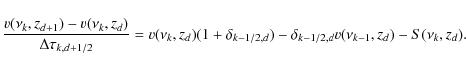
The difference form of the system of the equations in Eq. (7) is
where
| (A.5) | ||
| (A.6) | ||
| (A.7) |
Solving Eq. (A.4b) for
where
|
(A.9) |
Substituting Eqs. (A.8) into (A.4a), we derive a linear system of equations for

![$\displaystyle \qquad\qquad\qquad\qquad \left. +~ \frac{v(\nu_k,z_{d-1})}
{\Delta\tau_{k,d-1/2}(1+\delta_{k-1/2,d-1/2})}\right]$](/articles/aa/full_html/2010/11/aa14111-10/img157.png)

![$\displaystyle \qquad\qquad \quad +~ \frac{1}{\Delta\tau_{k,d}}\left[
\frac{\del...
...\delta_{k-1/2,d+1/2}u(\nu_{k-1},z_{d+1/2})}{1+\delta_{k-1/2,d+1/2}}\right]\cdot$](/articles/aa/full_html/2010/11/aa14111-10/img159.png)
This system should be supplemented by equations corresponding to the boundary and initial conditions. At the outer spatial boundary
|
(A.11) |
or, in a difference form
|
(A.12) |
The infalling radiation at the inner boundary is taken from the model atmospheres. The initial solution for
The velocity derivatives at the grid points are approximated as in the hydrodynamical code (see Krticka & Kubát 2001, Eq. (A.4a) therein). The derivatives in the middle points between grid points are calculated as the average of the derivatives at the grid points.
The system of algebraic equations Eq. (A.10) with boundary conditions is solved using the LAPACK package (http://www.cs.colorado.edu/ lapack, Anderson et al. 1999).
All Tables
Table 1:
Radius R*, mass M,
and the effective temperature
![]() of studied model stars.
of studied model stars.
Table 2: Comparison of calculated wind parameters derived using CMF and Sobolev line forces.
All Figures
| |
Figure 1: The ratio of the CMF to Sobolev line forces given by Eq. (13) as a function of the wind velocity plotted in the terms of the sound speed for two selected stars. The dashed-dotted line denotes a model with constant source function and constant level populations equal to their values at the sonic point. Arrows indicate the thermal speed of selected ions. |
| Open with DEXTER | |
| In the text | |
| |
Figure 2:
The line source function for resonance lines of O IV
at 790 Å, S V
at 786 Å, and Fe V
at 388 Å as a function of relative wind velocity. The source
function is plotted relative to its value at the sonic point |
| Open with DEXTER | |
| In the text | |
| |
Figure 3: The radial variation in the ratio of the CMF to Sobolev line forces in the wind model of Tc 1 central star with and without line overlaps. |
| Open with DEXTER | |
| In the text | |
| |
Figure 4: The ratio of the CMF to Sobolev line forces at radius r=5 R*in the Tc1 wind model in the dependence on the line shift. The value of hydrogen thermal speed is denoted in the figure. |
| Open with DEXTER | |
| In the text | |
|
|
Figure 5: Comparison of our derived mass-loss rates ( upper panel) and terminal velocities ( lower panel) of the central stars of planetary nebulae with those derived by Pauldrach et al. (2004). |
| Open with DEXTER | |
| In the text | |
| |
Figure 6: The mass-loss rate of HD 209975 in the models with additional turbulent line broadening relative to the models with zero turbulent velocity. |
| Open with DEXTER | |
| In the text | |
| |
Figure 7: The dependence of the radial velocity on radius for solutions with different boundary densities (mass-loss rates) close to the stellar surface for the model star 500-1. Each consecutive model (from down to up) differs by a factor of 1.5 in the mass-loss rate (thin lines). The thick line denotes the unique solution that smoothly intercepts the critical point. The dashed line denotes solution with the Sobolev line force. |
| Open with DEXTER | |
| In the text | |
Copyright ESO 2010
Current usage metrics show cumulative count of Article Views (full-text article views including HTML views, PDF and ePub downloads, according to the available data) and Abstracts Views on Vision4Press platform.
Data correspond to usage on the plateform after 2015. The current usage metrics is available 48-96 hours after online publication and is updated daily on week days.
Initial download of the metrics may take a while.