A&A 519, A103 (2010)

Microlensing in H1413+117: disentangling line profile emission and absorption in a broad absorption line quasar

D. Hutsemékers^1, - B. Borguet^1, - D. Sluse² - P. Riaud¹ - T. Anguita^2,3

1 - Institut d'Astrophysique et de Géophysique, Université de Liège, Allée du 6 Août 17, B5c, 4000 Liège, Belgium
2 - Astronomisches Rechen-Institut, Zentrum für Astronomie der Universität Heidelberg (ZAH), Mönchhofstr. 12-14, 69120 Heidelberg, Germany
3 - Departamento de Astronomía y Astrofísica, Pontificia Universidad Católica de Chile, Santiago, Chile

Received 4 September 2009 / Accepted 1 June 2010

Abstract
On the basis of 16 years of spectroscopic observations of the four components of the gravitationally lensed broad absorption line (BAL) quasar H1413+117, covering the ultraviolet to visible rest-frame spectral range, we analyze the spectral differences observed in the P Cygni-type line profiles and have used the microlensing effect to derive new clues to the BAL profile formation. We first find that the absorption gradually decreases with time in all components and that this intrinsic variation is accompanied by a decrease in the intensity of the emission. We confirm that the spectral differences observed in component D can be attributed to a microlensing effect lasting at least a decade. We show that microlensing magnifies the continuum source in image D, leaving the emission line region essentially unaffected. We interpret the differences seen in the absorption profiles of component D as the result of an emission line superimposed onto a nearly black absorption profile. We also find that the continuum source and a part of the broad emission line region are likely de-magnified in component C, while components A and B are not affected by microlensing. Differential dust extinction is measured between the A and B lines of sight. We show that microlensing of the continuum source in component D has a chromatic dependence compatible with the thermal continuum emission of a standard Shakura-Sunyaev accretion disk. Using a simple decomposition method to separate the part of the line profiles affected by microlensing and coming from a compact region from the part unaffected by this effect and coming from a larger region, we disentangle the true absorption line profiles from the true emission line profiles. The extracted emission line profiles appear double-peaked, suggesting that the emission is occulted by a strong absorber, narrower in velocity than the full absorption profile, and emitting little by itself. We propose that the outflow around H1413+117 is constituted by a high-velocity polar flow and a denser, lower velocity disk seen nearly edge-on. Finally, we report on the first ground-based polarimetric measurements of the four components of H1413+117.

Key words: gravitational lensing: micro - quasars: general - quasars: absorption lines - quasars: individual: H1413+117

1 Introduction

The broad absorption lines (BALs) observed in the spectra of quasars (or QSOs, quasi-stellar objects), blueshifted with respect to the broad emission lines (BELs), reveal massive, high-velocity outflows in active galactic nuclei (AGN). Such powerful winds can strongly affect the formation and evolution of the host galaxy, enrich the intergalactic medium, and regulate the formation of the large-scale structures (e.g. Silk & Rees 1998; Furlanetto & Loeb 2001; Scannapieco & Oh 2004; Scannapieco et al. 2005).

About 15% of optically selected quasars have BALs in their spectra (Reichard et al. 2003). Outflows may be present in all quasars if the wind is confined into a small solid angle so that BALs are only observed when the flow appears along the line of sight (Weymann et al. 1991; Gallagher et al. 2007). On the other hand, BAL QSOs could be quasars in an early evolutionary stage, washing out their cocoons (Voit et al. 1993; Becker et al. 2000).

Despite many high-quality observational studies, in particular from spectropolarimetry (Ogle et al. 1999), no clear view of the geometry and kinematics of the BAL phenomenon has emerged yet. While pure spherically symmetric winds appeared too simple to account for the variety of observations (Hamann et al. 1993; Ogle et al. 1999), equatorial disks, rotating winds, polar flows, or combinations thereof have been proposed more or less successfully to interpret the observations of individual objects or small groups of them (e.g. Murray et al. 1995; Schmidt & Hines 1999; Lamy & Hutsemékers 2004; Zhou et al. 2006). Given the large parameter space characterizing non spherically symmetric winds, BAL profile modeling must then be combined with other techniques to determine the outflow properties in individual objects (e.g. Young et al. 2007).

An interesting method that can bring independent information on the quasars' internal regions is the use of gravitational microlensing. Indeed, in a typical gravitationally lensed quasar, a solar mass star belonging to the lensing galaxy has an Einstein radius (the microlensing cross section) on the order of 10^-2 pc, which is comparable to the size of the continuum source. The microlens, moving across the quasar core in projection, can successively magnify regions of area , inducing spectroscopic variations that could be used to extract information on the quasar structure (Schneider et al. 1992, and references therein). Several studies, based on simulations, have demonstrated the interest of microlensing analyses for understanding BAL QSOs (Hutsemékers et al. 1994; Lewis & Belle 1998; Belle & Lewis 2000; Chelouche 2005).

H1413+117 is a BAL QSO of redshift showing typical P Cygni-type profiles, i.e., profiles where the absorption is not detached from the emission. Turnshek et al. (1988) discussed the spectrum of H1413+117 in detail and made the first attempts to disentangle the emission from the absorption assuming an intrinsic blue/red symmetry of the emission lines. H1413+117 is also a gravitationally lensed quasar constituted of four images (Magain et al. 1988; see Fig. 1). The lensing galaxy is faint and its redshift poorly known: indirect estimates give (Kneib et al. 1998) or (Goicoecha & Shalyapin 2010). Evidence of microlensing in component D has been suggested from both photometry and spectroscopy (Angonin et al. 1990; Østensen et al. 1997). In particular, Angonin et al. (1990) found that the equivalent width of the emission lines is systematically smaller in component D than observed in the other components, a result which can be interpreted by microlensing of the continuum source, the larger region at the origin of the emission lines being unaffected. This effect, which appeared to last at least a decade (Chae et al. 2001; Anguita et al. 2008a), offers the possibility to separate the microlensed attenuated continuum (i.e. the absorption profile) from the true emission line profile, thus providing new clues to the formation of BAL profiles (Hutsemékers 1993; Hutsemékers et al. 1994).

In the present paper, we homogeneously analyze the spectra of the four components of H1413+117 obtained from 1989 to 2005. The spectra cover the ultraviolet to visible rest-frame spectral range. In Sect. 3, we show that the spectral differences observed between the images can be consistently attributed to microlensing in spite of intrinsic variations. In Sect. 4, using a simple method, we separate the parts of the spectra affected and unaffected by microlensing, which basically correspond to the attenuated continuum and the emission lines. From these results, we derive a consistent view of the macro- and microlensing in H1413+117 (Sect. 5). Finally, with the ``pure'' absorption and emission profiles in hand, we discuss the formation of the BAL profiles and the implications for the geometry and the kinematics of the outflow (Sect. 6).

2 Data collection

Spectra of the four components of H1413+117 were gathered from archived and published data. Table 1 summarizes the characteritics of the spectra obtained over a period of 16 years, with the date of observation, the spectral range, the average resolving power , and the instrument used.

The visible spectra secured in 1989 with the bidimensional spectrograph SILFID at the Canada-France-Hawaii Telescope (CFHT) are described in Angonin et al. (1990) and Hutsemékers (1993). These spectra were obtained under optimal seeing conditions (0 6 FWHM). They provided the first spectroscopic evidence of microlensing in H1413+117.

A series of spectra were obtained in 1993-1994 with the Hubble Space Telescope (HST) feeding the Faint Object spectrograph (FOS). They cover the UV-visible spectral range (gratings G400H and G570H). These data are described in Monier et al. (1998). A second series of HST spectra, yet unpublished, were obtained in 2000 using the Space Telescope Imaging Spectrograph (STIS) and the G430L grating (principal investigator: Monier; proposal # 8127). All HST data were retrieved from the archive and reduced using standard procedures for long slit spectroscopy and prescriptions by Monier et al. (1998).

In 2005, visible spectra were obtained with the integral field unit of the Visible MultiObject Spectrograph (VIMOS) attached to the European Southern Observatory (ESO) Very Large Telescope (VLT). The data were obtained under medium quality seeing conditions (1 2 FWHM). Details on the observations and reductions are given in Anguita et al. (2008a). For this data set, it was not possible to separate the spectra of images A and B of H1413+117.

The 2005 near-infrared spectra obtained with the integral field spectrograph SINFONI at the VLT were retrieved from the ESO archive (principal investigator: Verma; proposal 075.B-0675(A)). Only the spectra obtained with the best seeing (0 5 FWHM on May 22, 2005 in the H and K spectral bands) are considered here. The pixel size was on the sky. The observations consist of four exposures per spectral band. The object was positionned at different locations on the detector for sky subtraction. The data were reduced using the SINFONI pipeline. Telluric absorptions were corrected using standard star spectra normalized to a blackbody. The individual spectra were extracted by fitting a 4-Gaussian function with fixed relative positions and identical widths to each image plane of the data cube using a modified MPFIT package (Markwardt 2009). Astrometric positions were taken from HST observations (Chantry & Magain 2007). The spectra which appeared affected by detector defects and/or important cosmic ray hits were discarded. The good spectra were finally filtered to remove remaining spikes.

In addition, we have observed H1413+117 on May 10, 2008 with the polarimetric mode of the Focal Reducer and low dispersion Spectrograph 1 (FORS1) installed at the Cassegrain focus of the VLT. Observations have been carried out with the filter, under excellent seeing conditions (0 6). Linear polarimetry has been performed by inserting in the parallel beam a Wollaston prism, which splits the incoming light rays into two orthogonally polarized beams, and a half-wave plate rotated to four position angles (e.g. Sluse et al. 2005). In order to measure the polarization of the four images, the MCS deconvolution procedure devised by Magain et al. (1998) has been applied. We used a version of the algorithm that allows for a simultaneous fit of different individual frames obtained with the same observational setup (Burud 2001). We constructed the PSF using a bright point-like object located 15 from H1413+117. Since this object is close to our target and is similar in brightness to the individual components of H1413+117, it provided a good estimate of the PSF. The Stokes parameters have been calculated from the photometry of the quasar lensed images derived from the deconvolution process.

Table 1:   Spectroscopic data.

3 Description of the spectra

At the redshift of H1413+117, spectra obtained in the UV-visible contain C IV  1548,1550, Si IV  1393,1402, N V  1238,1242, P V  1117,1128, O VI  1031,1037, Ly 1216 and Ly 1026, while the near-infrared spectra contain H 6563, H 4861 and [O III]  4959,5007 (Figs. 2 and 3). From the [O III] lines we measure the redshift z = 2.553. The UV resonance lines show typical P Cygni-type profiles with deep absorption while the Balmer lines show broad emission possibly topped with a narrower feature. Lyand Ly lines are weak due to absorption by the N V and O VI ions, respectively (e.g. Surdej & Hutsemékers 1987).

3.1 Evidence for microlensing

In Figs. 2 and 3, we compare the profiles of various spectral lines observed in the different images A, B, C, and D of H1413+117. A scaling factor is applied to superimpose at best the continua, considering in particular the continuum windows 4525-4545 Å and 5165-5220 Å (i.e. 1275-1280 Å and 1450-1470 Å rest-frame, Kuraszkiewicz et al. 2002). If the four images are only macrolensed, the line profiles observed in the spectra of the four components must be identical up to the scaling factor. On the other hand, line profile differences between some components may be indicative of microlensing, which is expected to magnify the - small - continuum region and not the - larger - broad emission line region.

We first note that the line profiles in components A and B are essentially identical up to the scaling factor. This suggests that neither A nor B are strongly affected by microlensing. The small difference observed in the [O III] lines may be related to the fact that the narrow line region could be partially resolved (Chantry & Magain 2007). The wavelength dependence of the scaling factor reveals higher dust extinction along the B line of sight than along the A one, as discussed in detail in Sect. 3.2. In the following we consider the average spectrum of components A and B, denoted AB, as the reference spectrum unaffected by microlensing effects. As seen in the upper panel of Fig. 2, the spectrum of H1413+117 changes regularly with time, suggesting intrinsic variations in the quasar outflow (this is further discussed in Sect. 3.3). These changes are observed in all components, indicating that the time scale of the intrinsic line profile variation is longer than the time delays between the four images. In fact, the longest time delay is not larger than one month according to the observations of Goicoecha & Shalyapin (2010) and in agreement with models (Kayser et al. 1990; Chae & Turnshek 1999).

The spectrum of component D is clearly different when compared to AB. After scaling the continua, the emission appears less intense in D. This behavior is observed at all epochs and in the different spectral lines, superimposed onto the intrinsic time variations seen in all components. This is a clear signature of a long-term microlensing effect in D with amplification of the continuum with respect to the emission lines. The timescale of the effect is in agreement with previous estimates, i.e. on the order of 10 years (e.g. Hutsemékers 1993). As first pointed out by Angonin et al. (1990), a difference is also observed in the absorption profiles. This difference is especially strong in the 1989 and 1993 spectra. This is a priori not expected since the region at the origin of the observed absorption lines has the same spatial extent as the continuum source. Differential microlensing of absorbing clouds smaller in projection than the continuum source has been proposed (Angonin et al. 1990). However the timescale of such an event is expected to be smaller than 1 year (Hutsemékers 1993), ruling out this interpretation. Instead, we interpret the difference in the absorption profiles as due to the superposition of an emission line onto a nearly black absorption profile (Sect. 6.1).

Although not as strong as in component D, spectral differences are also observed when comparing C to AB. After scaling the continua, the emission lines appear slightly stronger in C at all epochs, with a possible differential effect between the broad H and the narrower [O III] lines. This suggests that microlensing also affects component C, de-amplifying the continuum with respect to the emission lines.

The scaling factor used to fit the continuum of D to that one of AB clearly depends on wavelength. This can be explained either by chromatic microlensing (the source of UV continuum is less extended than the source of visible continuum and then more magnified), differential extinction (the extinction along the AB line of sight is higher than along the line of sight to D), wavelength-dependent dilution of the quasar continuum by the host galaxy light, or a combination thereof. Such a strong wavelength dependence of the scaling factor is not observed when comparing C to AB. The origin of this effect is further discussed in Sect. 5.2.

3.2 The extinction curve from A/B

Since images A and B are not significantly affected by microlensing, the wavelength dependence of their flux ratio can be interpreted in terms of differential extinction in the lensing galaxy. Figure 4 illustrates the observed flux ratio using all available spectroscopic data (slightly filtered and smoothed). Photometric data are superimposed. They were collected from Angonin et al. (1990), Østensen et al. (1997; the ratios are averaged per filter), Turnshek et al. (1997), Chae & Turnshek (2001), Kneib et al. (1998), Chantry & Magain (2007), MacLeod et al. (2009).

There is a lot of dispersion in the measured flux ratios which arises not only from inacurracies in the data but also from a possible combined effect of intrinsic photometric variations and time delay (cf. Østensen et al. 1997). A clear trend is nevertheless observed, indicating higher extinction along the line of sight to image B, as suggested by Turnshek et al. (1997). The flux ratio is reasonably well modeled using

where is the difference of extinction between the A and B line of sights measured in the B filter and the extinction curve tabulated in Pei (1992), redshifted to the lens redshift (Kneib et al. 1998). Since no obvious 2200 Å feature typical of the Milky Way extinction is observed at 2.3 m^-1 (Fig. 4), we adopt a SMC-like extinction curve. A reasonably good fit is obtained with and (Fig. 4). With (Goicoecha & Shalyapin 2010) a similar fit is obtained with . For (1.88), the lines of sight to images A and B sample regions of the lens galaxy located at respectively 4.9 (5.2) kpc and 6.0 (6.4) kpc from the galaxy center, adopting the astrometry of Chantry & Magain (2007) and assuming a flat cosmology with and  km s^-1 Mpc^-1. The flux ratio measured by MacLeod et al. (2009) at 11 m in the mid-infrared, i.e. at wavelengths were both extinction and microlensing are expected to be negligible, is compatible with the extinction corrected flux ratio we derive, although marginally higher.

3.3 Intrinsic line profile variations

Time variations in the absorption line profiles of BAL quasars are not uncommon (Barlow et al. 1989,1992; Gibson et al. 2008). In H1413+117, Turnshek et al. (1988) reported a deepening of the Si IV BAL between 1981 and 1985. On the contrary, between 1989 and 2005 (Fig. 2), variations are observed as a gradual decrease of the depth of the BAL high-velocity part, the deepest component of the profile being essentially unaffected. Variations appear more complex in Si IV than in C IV, affecting a larger part of the absorption profile (see also Fig. 6).

The strongest change occurs between 1989 and 1993 and corresponds to an increase of the luminosity (Remy et al. 1996; Østensen et al. 1997). Moreover, stronger absorption is accompanied by stronger emission, which is an indication that resonance line scattering can play an important role in the emission line formation. In the C IV line of the AB spectrum, the high-velocity absorption appears 15% larger in 1989 than in 2005 while the emission is 25% more intense. In the framework of resonance scattering where each absorbed photon is re-emitted, this may suggest that the high-velocity outflow has more scattering material perpendicular to the line of sight than absorbing material along the line of sight. This also requires a large covering factor.

4 Decomposition of the line profiles

4.1 The method

We follow a method similar to that used in Sluse et al. (2007). Assuming that the observed spectra F_i of the different images are made of a superposition of a spectrum which is only macrolensed and of a spectrum which is both macro- and microlensed, it is possible to extract the components and by using pairs of observed spectra. Indeed, considering a line profile, we can write

where M=M₁/M₂ is the macro-amplification ratio between images 1 and 2 and the micro-amplification factor of image 1. We assume image 2 not affected by microlensing. To extract and when M is not known a priori, these equations can be conveniently rewritten

where . Considering the line profiles as the sum of a continuum (absorbed or not in the blue) and an emission profile, we write , , and then

Up to a scaling factor, only depends on A, while only depends on M (Eqs. (4) and (5)). A is the scaling factor between the F₁ and F₂ continua: . It can be accurately determined as the value for which in the continuum adjacent to the line profile, where  (Eq. (6)). Assuming A constant across the line profile, then only contains a contribution from the emission profile. Under the assumption that at least a portion of the observed emission profile is only macro-amplified (i.e. not micro-amplified), the macro-amplification factor can be estimated as the value of M such that over that part of the line profile (Eq. (7), see also Appendix A). The micro-amplification factor of the continuum is then estimated at the wavelength of the line profile: . On the other hand, if the emission line is amplified exactly like the continuum, microlensing cannot be distinguished from macrolensing.

Equations (6) and (7) show that if the emission profile is only macro-amplified (i.e. if ), only contains the underlying continuum , while contains the full emission profile . If the emission profile is micro-amplified to some extent, parts of it will appear in both and (see Appendix A). More specifically, can be seen as the part of the emission profile which is not only macro-amplified, and as the part of the emission profile which is not amplified like the continuum.

The micro-amplification factor and the macro-amplification factor M possess some specific chromatic behaviors. While is assumed constant over the small wavelength range spanned by a line profile, it can be different at the wavelengths corresponding to different line profiles. Indeed, the micro-amplification of the continuum is related to the effective size of the continuum source which can be wavelength-dependent. The macro-amplification factor Mmay also contain a wavelength-dependent contribution due to differential extinction in the lensing galaxy, since extinction, like macrolensing, acts on the line profile as a whole. Finally, concerning the time dependence properties, M is expected to remain identical at different epochs of observation while can be time-dependent.

4.2 The results

4.2.1 Line profile decomposition from the (D, AB) pair

Table 2:   Amplification factors determined from the (D, AB) pair.

We extract and from the spectra of H1413+117 using and in Eqs. (4) and (5). We have M < 1and since D is fainter than AB and its continuum amplified (Sect. 3.1). A is computed as the value for which in the continuum windows adjacent to the line profiles (cf. Sect. 3.1). Within the uncertainties, A is the inverse of the scaling factor determined in Figs. 2 and 3. M is computed as the largest value for which over the whole line profile. For the resonance line profiles, the continuum may be completely absorbed at some wavelengths such that must also be larger than zero. Measurements of A and M are given in Table 2 with . Taking into account the noise and possible contaminating features in the observed spectra, a range of acceptable values is obtained which provides a rough estimate of the uncertainties. These are typically 2-3% for A and 4-10% for M. As expected, the macro-amplification factor M is independent of the epoch of observation, the dispersion of the values being in agreement with the uncertainties. The temporal variation of A then essentially comes from the variation of the micro-amplification of the continuum. This is shown in Fig. 5. This figure also suggests that, within the uncertainties, there is no significant wavelength dependence of M due to a differential reddening between AB and D (see also Sect. 5.1).

With the measured A and M, we then compute and from Eqs. (4) and (5). The results of the line profile decompositions are given in Figs. 6 to 8. Over large parts of the emission profile (mainly in the wings), . This indicates that at least a part of the observed emission line profile is unaffected by microlensing and that M actually represents the macro-amplification factor. We emphasize that the derived and profiles are robust against small changes of A or M.

Figure 6 illustrates the spectral decomposition for the Si IV-C IV region. Although different values of A(or ) are found at different epochs, the extracted spectra are remarkably consistent. The microlensed part of the spectrum, , contains the continuum with the full absorption profiles as well as a small contribution from the core (not the wings) of the emission profiles. The bulk of the emission lines appears in the macrolensed-only part of the spectrum , clearly showing a two-peak structure in C IV (at 5350 Å and 5500 Å). Recall that shows the flux emitted from a large region of the quasar (much larger than the Einstein radius of the microlens) whereas shows the flux emitted from a smaller region (comparable to and smaller than the Einstein radius). Interestingly enough, the small part of the emission profile observed in is the core, i.e. the low-velocity part. The temporal variations of the absorption are particularly well seen in the spectrum of Si IV.

The rest-frame UV spectra, and more particularly the Ly + N V region, are similarly analyzed (Fig. 7). Although the decomposition is less accurate due to structures in the continuum blueward of Ly (possibly due to narrow absorption features and inaccuracies in the wavelength calibration), the extracted spectra and show the same qualitative behavior as observed in the C IV and Si IV line profiles.

Figure 8 shows the decomposition for the H + [O III] and H line profiles. The micro-amplified spectrum is clearly a flat continuum in the H + [O III] spectral region while there is some evidence that the core (and not the wings) of the H emission line is micro-amplified.

4.2.2 Line profile decomposition from the (C, AB) pair

The same kind of analysis can be done using the pair (C, AB). However the line profile differences are more subtle (cf. Figs. 2 and 3) so that the value of M is closer to the value of A (i.e.  closer to 1) in Eqs. (4) and (5), making the extracted spectra noisier. Only the spectra obtained in 2000, which show the most conspicuous profile differences, are considered here. A de-magnification of the continuum explains the observations (Sect. 3.1) and the resulting and are illustrated in Fig. 9. They are roughly similar to those derived from the pair (D, AB) but the part of the emission profile which is micro-amplified is different. While only a small part of the core of the emission is seen in the profile derived from the (D, AB) pair, the red wing of the emission profile is also observed in computed from (C, AB). This red wing and the blue emission peak are not seen in , suggesting that the high-velocity component of the C IV resonance line is micro-deamplified like the continuum. This is not unexpected since, for a given Einstein radius, demagnification regions with relatively smooth variations can extend on larger scales than amplification regions (e.g. Lewis & Ibata 2004). The emission line core, which appears in both and , should originate, at least in part, from a region more extended than the high-velocity component.

From the 2005 near-infrared spectra (the decomposition of which is not shown), we measure A = 0.74 for both the H+[O III] and H regions. The condition is verified at the wavelengths of H or H with , while is obtained at the wavelength of the [O III] lines with . The latter value is comparable to the value of M derived from the UV-visible resonance lines. Although the narrow line region may be partially resolved (Chantry & Magain 2007), the [O III] emission lines are expected to originate from a larger region and then less affected by microlensing, making a more plausible estimate. In this case, with for the micro-amplification factor of the continuum, the Balmer emission lines do appear in both and . This means that they are also micro-deamplified although not as much as the continuum.

5 Lensing in H1413+117

5.1 The macro-amplification factors

In principle, the variation of M with the wavelength can be attributed to differential extinction. Unfortunately, for the (D, AB) pair, the wavelength dependence is not clear enough to extract an extinction curve, given the uncertainties on the determination of M(Fig. 5 and Table 2). The results nevertheless suggest that the differential extinction between AB and D is lower than between A and B for which the extinction at Lyis 1.2 times the extinction at H(Fig. 4). As a consequence, the value M(D, AB determined at the wavelength of H, i.e. in the reddest part of our spectra, should not differ from the true macro-amplification factor by more than 2%.

For the (C, AB) pair, we conservatively adopt M(C, AB at the wavelength of H. Comparing with M(C, AB and M(C, AB at the wavelengths of Ly and C IV, respectively (Fig. 9), M(C, AB) might be slightly wavelength dependent, providing marginal evidence that extinction is lower for C than for AB. Since the differential extinction remains low, we also assume that it does not affect the macro-amplification factor determined at the wavelength of H by more than 2%.

The flux ratios with respect to component A are then / .02 (Fig. 4), / .10 and / .04. The fact that / and / are different from the values estimated from photometry is due to a significant de-amplification of the C continuum and to a significant amplification of the D continuum, as derived from the analysis of the spectral lines. This emphasizes the need to properly correct for microlensing before interpreting the flux ratios.

MacLeod et al. (2009) determined , and at 11 m in the mid-infrared, i.e., where microlensing and extinction are thought to be negligible. Although only marginally different, the flux ratios of the B and C components relative to A seem slightly smaller than ours. If real, the origin of such a discrepancy is not clear but could be related to the intense starburst activity detected in the host galaxy of H1413+117 (Lutz et al. 2007; Bradford et al. 2009), which possibly contaminates with PAH emission the 11.2 m (3.2 m rest-frame) flux measurements.

5.2 Microlensing of the continuum source

The micro-amplification factor determined in component D depends on both the date and the wavelength (Table 2).

Considering the Si IV-C IV spectral region, the strongest variation of occurs between 1989 and 1993 (see also Figs. 2 and 6). It roughly corresponds to a relative photometric variation between A and D which can be observed in the V light curves of H1413+117 presented by Remy et al. (1996) and Østensen et al. (1997), superimposed onto the common intrinsic variation of the 4 components. Between 1993 and 2000, the variation of is weaker, in agreement with the HST photometry in the F555W filter reported by Turnshek et al. (1997) and Chae et al. (2001).

At a given epoch, decreases with increasing wavelength, suggesting chromatic magnification of the continuum source. This is best seen in the 2005 data (obtained within a 2 month interval) which span the largest wavelength range. We emphasize that , when determined from the line profiles, is not contaminated by differential extinction (Sect. 4.1). In Fig. 10, we plot the values of as a function of the wavelength of observation in the quasar rest-frame.

The magnification of an extended source close to a caustic can be written

where is the source radius, the Einstein radius of the microlens projected onto the source plane, g is a constant on the order of unity, a function which depends on the distance to the caustic and a constant ``background'' magnification (e.g. Schneider et al. 1992; Witt et al. 1993). In the framework a simple model where the continuum is emitted by a Shakura-Sunyaev (1973) thin accretion disk thermally radiating, (e.g. Poindexter et al. 2008) such that we may expect

As seen in Fig. 10, this model nicely reproduces the data using C = -0.55 and assuming for simplicity (i.e. no background (de- )magnification), supporting the idea of chromatic magnification of a continuum emitted by a Shakura-Sunyaev accretion disk.

In principle, we could have used the Ly+N V and the C III] 1909 emission lines, also present in the 2005 visible spectra, to measure at other wavelengths. Although tentative estimates do agree with the observed trend, the quality of the data is not sufficient to derive reliable values of at these wavelengths, due to the insufficient spectral resolution in the complex Ly+N V region and to the fact that the C III] line is truncated. Clearly, with better quality data, it could be possible to separate M and at other wavelengths using additional line profiles and thus derive the temperature profile of the accretion disk.

From the value of the constant C, we can derive a rough estimate of the size of the continuum source: . The Einstein radius is computed to be  pc using z_l = 1.0, a flat cosmology, and H  km s^-1 Mpc^-1. M is the mass of the microlens. Then,  pc at the rest-frame UV wavelength m. This limits tightens to  pc with z_l = 1.88. These values agree with the radii obtained for the lensed quasars HE1104-1805 and Q2237+0305 on the basis of their photometric variability due to microlensing (e.g. Poindexter et al. 2008; Eigenbrod et al. 2008; Anguita et al. 2008b).

Dilution of the quasar continuum - microlensed - by the host galaxy light - not microlensed - can affect the interpretation of the wavelength dependence of . Denoting the ratio of the host and quasar continua at a given wavelength, we find that the micro-amplification factor of the quasar continuum is related to the measured by

if the host galaxy is unresolved and macrolensed as the quasar (i.e. if ), or by

if the host galaxy is resolved and not macrolensed (i.e. if assuming the host contained in the measurement aperture). Dilution by the host galaxy is expected to be stronger in the rest-frame visible-infrared than in the ultraviolet. In the rest-frame visible of a luminous high-redshift object, (e.g. Schramm et al. 2008) so that does not differ from by more than 5% (even less if the host is partially resolved). This is negligible and within the uncertainties.

5.3 Microlensing of a scattering region?

Chae et al. (2001) have obtained the first polarization mesurements of the four images of H1413+117 using the HST. The F555W filter was used. They noted that, in March 1999, the polarization degree of component D might be higher that the polarization degree of the other components (Table 3). From this result, they suggested that microlensing also affects the scattering region. The measurements obtained in June 1999 possibly indicate an intrinsic variation of the polarization observed in all components. Similar variations have been reported by Goodrich & Miller (1995).

Table 3:   Polarimetry of the four images.

Taking advantage of an excellent seeing, we were able to measure the polarization of the 4 components of H1413+117 in the V filter, from the ground. Our measurements are also reported in Table 3. Within the uncertainties, the polarization degree of components A, B and C do agree with the March 1999 values of Chae et al. (2001), while the polarization degree of component D does not. Instead, we find that the difference between the polarization degrees measured in A and C and those ones measured in B and D is significant. The difference between A and B is especially intriguing since we found no significant microlensing effect neither in A nor in B (at least before 2005). Possible interpretations could involve the polarization due to an extended scattering region resolved by the macrolens (possibly in the host galaxy, see Borguet et al. 2008), or a differential polarization induced by aligned dust grains in the lens galaxy. More data are clearly needed to correctly understand the meaning of these measurements.

6 Consequences for the BAL formation

In the previous sections we derived a consistent picture of microlensing in H1413+117, showing that the continuum of component D (or more precisely all the regions of the quasar located in a cylinder of diameter oriented along the line of sight and containing the continuum source) is magnified with respect to the more extended regions at the origin of the emission lines. This allowed us to disentangle the absorption part of the BAL profiles, essentially , from the emission part, essentially (Figs. 6 to 8). The observed profiles are equal to the sum of the and spectra (Eq. (3)). The separation is robust against the uncertainties of the amplification factors. It is however not perfect since emission which originates from regions close to the continuum source in projection appears in  . Selected spectra are illustrated in Fig. 11 on a velocity scale.

The absorption profile of the C IV BAL appears nearly black extending from  km s^-1 to  km s^-1. It is especially interesting to note that the flow does not start at v = 0 in the rest-frame defined by the [O III] emission lines. The part of the profile between -8000 and -10 000 km s^-1 is clearly variable between 1993 and 2000, showing a smaller depth in 2000. At a given epoch (1993-1994), the absorption appears stronger in N V and weaker in Si IV; this is best seen in the velocity range -2000 to -4000 km s^-1 and indicates an ionization dependence of the optical depth. The extracted emission profiles show a double-peaked structure which extends to the blue as far as the absorption profile does. The blue peak at -8000 km s^-1 appears much fainter than the red peak at -1000 km s^-1. The full emission profile (represented by the green line in Fig. 11) is roughly centered on the onset velocity of the flow (-2000 km s^-1), thus blueshifted with respect to the [O III] rest-frame. In fact, the full absorption + emission line profile appears in a rest-frame blueshifted by -2000 km s^-1 with respect to the rest-frame defined by the [O III] emission lines. H, on the other hand, appears redshifted (Fig. 3). Although not clearly understood, these line shifts are common in quasars (e.g. Corbin 1990; McIntosh et al. 1999) and particularly strong in BAL QSOs (Richards et al. 2002), in agreement with our observations. Interestingly enough, Nestor et al. (2008) found a deficit of intrinsic C IV Narrow Absorption Line (NAL) systems at outflowing velocities lower than 2000 km s^-1, possibly due to overionization close to the accretion disk.

The shape of the emission suggests that it is occulted by a strong absorber, narrower in velocity than the full absorption profile, and emitting little by itself. Very similar absorption and emission profiles are produced in the outflow model of Bjorkman et al. (1994) proposed for early-type stars. We build on this model to interpret our observations. A toy model, detailed in Appendix B, is used for illustrative purposes (a full radiative transfer modeling is beyond the scope of the present paper; it is presented in Borguet & Hutsemékers 2010, where details on the flow geometry are also given). We assume that the outflow in H1413+117 is constituted of two components: a quasi-spherically symmetric ``polar'' outflow, and a denser disk seen nearly edge-on. The equatorial disk expands slower than the polar wind and partly covers it. The polar outflow produces typical P Cygni line profiles constituted of the superposition of a deep absorption extending from -2000 to roughly -10 000 km s^-1 and a symmetric emission due to resonantly scattered photons (e.g. Lamers & Cassinelli 1999). This emission (assumed Gaussian shaped for simplicity) is centered on  km s^-1 and extends from -10 000 to +6000 km s^-1. Both the remaining continuum and the emission from the polar wind are absorbed in the equatorial disk. A double-peaked emission line is then produced (Fig. 11), little emission being expected from the edge-on disk. As we can see from Fig. 11, this simple model is able to reproduce the main characteristics of the intrinsic emission line profiles extracted from the microlensing analysis. Since the disk is expected to also absorb the continuum, its absorption profile must be contained within the total polar+equatorial absorption profile, as illustrated. Variability of the polar outflow optical depth will generate variations at the high velocity end of the absorption accompanied by a change in the resonantly scattered emission, as observed (Sect. 3.3; see also Bjorkman et al. 1994, for simulations). Note that two-component winds have good theoretical grounds (e.g. Murray et al. 1995; Proga & Kallman 2004) and are supported by many observations interpreted with either disks or polar flows (cf. Sect. 1).

Spectropolarimetric observations of H1413+117 (e.g. Goodrich & Miller 1995; Lamy & Hutsemékers 2004) provide additional evidence favoring this kind of scenario. First, the polarization angle rotates within the absorption line profiles, suggesting the existence of at least two sources and/or mechanisms of polarization. The polar outflow and the disk, expected to produce perpendicular polarizations, can play this role, especially in the case of BAL QSOs with P Cygni-type profiles (Goodrich 1997; Hutsemékers et al. 1998; Lamy & Hutsemékers 2004). Furthermore, the absorption in the polarized spectrum is clearly narrower than the absorption in the direct spectrum (this is best observed in Fig. 3 of Goodrich & Miller 1995), supporting the existence of a slowly expanding equatorial disk which absorbs the polar-scattered flux.

6.1 Microlensing in the BAL

The difference observed in the BAL profiles of images AB and D (best seen in C IV, Fig. 2) can also be interpreted in the framework of this outflow model. In 1989 and 1993, the intrinsic absorption at 5330 Å (-9000 km s^-1) due to the high-velocity ``polar'' outflow is nearly black (Figs. 6 and 11). In classical P Cygni line profile formation (e.g. Lamers & Cassinelli 1999; Hutsemékers & Surdej 1990), this absorption is partially filled in with emission resonantly scattered at the same velocity (the blueward peak of the intrinsic emission, not absorbed by the slower disk, and seen in Figs. 6 and 11). Since the emission line and the absorbed continuum react differently to the magnification by the microlens, a spectral difference is observed in the high-velocity part of the BALs seen in AB and D. Later, in 2000 and 2005, the high-velocity part of the BAL profile is less optically thick: the absorption is not as deep as in the nineties and the blue wing of the resonantly scattered emission which fills in the absorption is accordingly weaker (the blue emission peak appears narrower or less intense in 2000 and 2005, Figs. 6 and 11). As a consequence, the microlens-induced spectral difference observed in the high-velocity part of the BALs appears smaller at these epochs.

7 Conclusions

Using 16 years of spectroscopic observations of the 4 components of the gravitationally lensed BAL quasar H1413+117, we derived the following results.

-

The strength of the BAL profiles gradually decreases with time in all components. This intrinsic variation is accompanied by a decrease of the intensity of the emission.

-

The spectral differences observed in component D can be attributed to a long-term microlensing effect, in agreement with previous studies. This effect consistently magnifies the continuum source of image D, leaving the broad emission line region essentially unaffected. We also find that the continuum of component C is most likely de-magnified, while components A and B are not affected by microlensing. Differential extinction is found between A and B.

-

Using a simple decomposition method to separate the part of the line profiles affected by microlensing from the part unaffected by this effect, we were able to disentangle the intrinsic absorption (affected) from the emission line profile (unaffected). Consistent results are obtained for the different epochs of observation.

-

Considering the macro- and micro-amplification factors estimated with this method, we obtain a coherent view of lensing in H1413+117. In particular, we show that microlensing of the D continuum source has a chromatic dependence which is compatible with a continuum emitted by a standard Shakura-Sunyaev accretion disk.

-

To interpret the extracted absorption and emission line profiles, we propose that the outflow from H1413+117 is constituted of a high-velocity polar flow (at the origin of the intrinsic variations) and a dense disk expanding at lower velocity and seen nearly edge-on. This is in agreement with spectropolarimetric data and supports the idea that BAL outflows can have large covering factors.

In our analysis, we focused on the most robust results. Several interesting questions nevertheless remain opened, requiring more observations or a full radiative transfer modeling. In particular, why does the polarization of the different components apparently differ? Is the scattering region actually magnified? High-quality spectropolarimetry of the four images of H1413+117 may solve this issue and bring more informations on the nature of the ouflow. As seen in Figs. 6 to 9, different parts of the emission line profiles appear micro-(de)amplified in components C and D. Detailed line profile calculations are needed to understand the origin of this micro-amplified emission and shed light on the outflow kinematics. With excellent signal-to-noise spectra, it would also be possible to better use the microlensing effect observed in component C.

Acknowledgements

It is a pleasure to thank Virginie Chantry for providing us with the image illustrated in Fig. 1. A fellowship from the Alexander von Humboldt Foundation to D.S. is gratefully acknowledged.

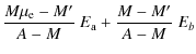
Appendix A: Example of a line profile decomposition

We consider a line profile constituted of an underlying continuum (absorbed or not at some wavelengths) and an emission profile . We assume the continuum micro-amplified by a constant factor , the component  of the emission micro-amplified by a constant factor , and the component E_b unaffected by microlensing. We consider a typical case with . If M is the relative macro-amplification factor between images 1 and 2, we have

Using these expressions with and in Eqs. (4) and (5), we find

with , and . As expected, contains the emission profile E_b unaffected by microlensing, contains the continuum, and both and contain a part of the micro-amplified emission profile . Up to a scaling factor, the micro-amplified profile is given by .

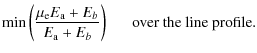
To effectively compute Eqs. (4) and (5) and to determine the profile of , we need to know M (or ). Practically, we consider M as a free parameter in Eq. (5) and, by varying it, we adopt the value of M closest to Asuch that at all wavelengths (Eq. (7)). This is equivalent to adopt a value of as close as possible to 1, thus ensuring that the macro- and micro-amplifications are best separated (see also Sluse et al. 2007). Unless , this method provides a reasonably accurate estimate of M, and then of . Indeed, denoting the free parameter M' and using expressions A.1 and A.2 in Eq. (5), we write

such that is satisfied when

with

If and at some wavelengths, then and M = M'. This means that M can be derived empirically when at least a portion of the observed emission line profile is not micro-amplified. In fact this is formally always true. Indeed, if , the whole profile would be micro-amplified by i.e. macro-amplified by instead of M, which is inconsistent with an optimal separation of macro- and micro-lensing. It should nevertheless be kept in mind that if the emission line is amplified just like the continuum, microlensing cannot be distinguished from macrolensing. Fortunately, it is realistic to assume that a portion - even a very small one - of the observed emission line profile is not micro-amplified given the large size of the emission line region compared to the source of the continuum and to a typical Einstein radius. This hypothesis can be verified as follows: if we notice that and over a certain wavelength range, then we must have M' = M and . Indeed, combining Eqs. (A.5) and (A.6), we find that when then either must be proportional to E_b over that wavelength range - which is unlikely since and E_b are meant to originate from different emission regions - or .

Appendix B: The absorption / emission toy model

For a given line profile, we adopt for the disk optical depth the functional form

where w is the velocity. is the position of the center of the absorption line i, and the width taken identical for all lines. The sum is computed over the 2 or 3 lines which constitute a line profile, with the appropriate weights . Similarly, we adopt for the unabsorbed emission line profile

The disk absorption profile is computed as and the emission line profile absorbed by the disk as . The total absorption of the continuum must be equal to the absorption in the polar flow multiplied by the absorption in the disk. Although not computed, it can be obtained by inverting the observed intrinsic absorption profile.

For all line profiles shown in Fig. 11, we use 5000 km s^-1,  km s^-1, 2000 km s^-1,  km s^-1, i=1 corresponding to the reddest line of the profiles, the position of the other ones being fixed by the doublet separation and/or by the Ly - N V velocity separation. and are choosen to fit the observations. The parameters are not unique and may be different at other epochs.

References 

• Angonin, M.-C., Vanderriest, C., Remy, M., & Surdej, J. 1990, A&A, 233, L5
• Anguita, T., Faure, C., Yonehara, A., et al. 2008a, A&A, 481, 615
• Anguita, T., Schmidt, R. W., Turner, E. L., et al. 2008b, A&A, 480, 327
• Barlow, T. A., Junkkarinen, V. T., & Burbidge, E. M. 1989, ApJ, 347, 674
• Barlow, T. A., Junkkarinen, V. T., Burbidge, E. M., et al. 1992, ApJ, 397, 81
• Becker, R. H., White, R. L., Gregg, M. D., et al. 2000, ApJ, 538, 72
• Belle, K. E., & Lewis, G. F. 2000, PASP, 112, 320
• Bjorkman, J. E., Ignace, R., Tripp, T. M., & Cassinelli, J. P. 1994, ApJ, 435, 416
• Borguet, B., & Hutsemékers, D. 2010, A&A, 515, A22
• Borguet, B., Hutsemékers, D., Letawe, G., Letawe, Y., & Magain, P. 2008, A&A, 478, 321
• Bradford, C. M., Aguirre, J. E., Aikin, R., et al. 2009, ApJ, 705, 112
• Burud, I. 2001, Ph.D. Thesis
• Chae, K.-H., & Turnshek, D. A. 1999, ApJ, 514, 587
• Chae, K.-H., Turnshek, D. A., Schulte-Ladbeck, R. E., Rao, S. M., & Lupie, O. L. 2001, ApJ, 561, 653
• Chantry, V., & Magain, P. 2007, A&A, 470, 467
• Chelouche, D. 2005, ApJ, 629, 667
• Corbin, M. R. 1990, ApJ, 357, 346
• Eigenbrod, A., Courbin, F., Meylan, G., et al. 2008, A&A, 490, 933
• Furlanetto, S. R., & Loeb, A. 2001, ApJ, 556, 619
• Gallagher, S. C., Hines, D. C., Blaylock, M., et al. 2007, ApJ, 556, 619
• Gibson, R. R., Brandt, W. N., Schneider, D. P., & Gallagher, S. C. 2008, ApJ, 675, 985
• Goicoechea, L. J., & Shalyapin, V. N. 2010, ApJ, 708, 995
• Goodrich, R. W., & Miller, J. S. 1995, ApJ, 448, L73
• Goodrich, R. W. 1997, ApJ, 474, 606
• Hamann, F., Korista, K. T., & Morris, S. L. 1993, ApJ, 415, 541
• Hutsemékers, D. 1993, A&A, 280, 435
• Hutsemékers, D., & Surdej, J. 1990, ApJ, 361, 367
• Hutsemékers, D., Surdej, J., & van Drom, E. 1994, Ap&SS, 216, 361
• Hutsemékers, D., Lamy, H., & Remy, M. 1998, A&A, 340, 371
• Kayser, R., Surdej, J., Condon, J. J., et al. 1990, ApJ, 364, 15
• Kneib, J.-P., Alloin, D., & Pello, R. 1998, A&A, 339, L65
• Kuraszkiewicz, J. K., Green, P. J., Forster, K., et al. 2002, ApJS, 143, 257
• Lamers, H. J. G. L. M., & Cassinelli, J. P. 1999, Introduction to stellar winds (Cambridge University Press)
• Lamy, H., & Hutsemékers, D. 2004, A&A, 427, 107
• Lewis, G. F., & Belle, K. E. 1998, MNRAS, 297, 69
• Lewis, G. F., & Ibata, R. A. 2004, MNRAS, 348, 24
• Lutz, D., Sturm, E., Tacconi, L. J., Valiante, E., et al. 2007, ApJ, 661, L25
• MacLeod, C. L., Kochanek, C. S., & Agol, E. 2009, ApJ, 699, 1578
• Magain, P., Surdej, J., Swings, J.-P., Borgeest, U., & Kayser, R. 1988, Nature, 334, 325
• Magain, P., Courbin, F., & Sohy, S. 1998, ApJ, 494, 472
• Markwardt, C. B. 2009, XVIII ASP Conf. Ser., 411, 251
• McIntosh, D. H., Rix, H.-W., Rieke, M. J., & Foltz, C. B. 1999, ApJ, 517, L73
• Monier, E. M., Turnshek, D. A., & Lupie, O. L. 1998, ApJ, 496, 177
• Murray, N., Chiang, J., Grossman, S. A., & Voit, G. M. 1995, ApJ, 451, 498
• Nestor, D., Hamann, F., & Rodriguez Hidalgo, P. 2008, MNRAS, 386, 2055
• Ogle, P. M., Cohen, M. H., Miller, J. S., et al. 1999, ApJS, 125, 1
• Østensen, R., Remy, M., Lindblad, P. O., et al. 1997, A&AS, 126, 393
• Pei, Y. C. 1992, ApJ, 395, 130
• Poindexter, S., Morgan, N., & Kochanek, C. S. 2008, ApJ, 673, 34
• Proga, D., & Kallman, T. R. 2004, ApJ, 616, 688
• Reichard, T. A., Richards, G. T.; Hall, P. B.; et al. 2003, AJ, 126, 2594
• Remy, M., Gosset, E., Hutsemékers, D., Revenaz, B., & Surdej, J. 1996, Astrophysical Applications of Gravitational Lensing, 173, 261
• Richards, G. T., Vanden Berk, D. E., Reichard, T. A., et al. 2002, AJ, 124, 1
• Saha, P., & Williams, L. L. R. 2004, AJ, 127, 2604
• Scannapieco, E., & Oh, S. P. 2004, ApJ, 608, 62
• Scannapieco, E., Silk, J., & Bouwens, R. 2005, ApJ, 635, L13
• Schmidt, G. D., & Hines, D. C. 1999, ApJ, 512, 125
• Schneider, P., Ehlers, J., & Falco, E. E. 1992, Gravitational Lenses (Berlin, Heidelberg, New York: Springer-Verlag)
• Schramm, M., Wisotzki, L., & Jahnke, K. 2008, A&A, 478, 311
• Shakura, N. I., & Sunyaev, R. A. 1973, A&A, 24, 337
• Silk, J., & Rees, M. 1993, A&A, 331, L1
• Sluse, D., Hutsemékers, D., Lamy, H., Cabanac, R., & Quintana, H. 2005, A&A, 433, 757
• Sluse, D., Claeskens, J.-F., Hutsemékers, D., & Surdej, J. 2007, A&A, 468, 885
• Surdej, J., & Hutsemékers, D. 1987, A&A, 177, 42
• Turnshek, D. A., Lupie, O. L., Rao, S. M., Espey, B. R., & Sirola, C. J. 1997, ApJ, 485, 100
• Turnshek, D. A., Grillmair, C. J., Foltz, C. B., & Weymann, R. J. 1988, ApJ, 325, 651
• Voit, G. M., Weymann, R. J., & Korista, K. T. 1993, ApJ, 413, 95
• Witt, H. J., Kayser, R., & Refsdal, S. 1993, A&A, 268, 501
• Weymann, R. J., Morris, S. L., Foltz, C. B., & Hewett, P. C. 1991, ApJ, 373, 23
• Young, S., Axon, D. J., Robinson, A., Hough, J. H., & Smith, J. E. 2007, Nature, 450, 74
• Zhou, H., Wang, T., Wang, H., et al. 2006, ApJ, 639, 716 

Footnotes

... quasar

Based on observations made with the Canada-France-Hawaii Telescope (Hawaii), with ESO Telescopes at the Paranal Observatory (Chile) and with the NASA/ESA Hubble Space Telescope, and obtained from the data archive at the Space Telescope Institute. ESO program ID: 074.A-0152, 075.B-0675, 081.A-0023.

...

Maître de Recherches du FNRS.

...

Boursier du FNRS.

... models

We also estimate small time delays, typically less than 10 days, considering a classical singular isothermal ellipsoid (SIE)+shear model, a SIE+shear+galaxy model proposed by MacLeod et al. (2009), as well as using pixellated models with a symmetric mass distribution (Saha & Williams 2004).

... microlensing

It is always possible to write where = max( ).

...M

As discussed in Sect. 4.1, the factor A and then the profile of are more easily determined.

... micro-lensing

The amplification factors can be renormalized as follows: , and . Note that = min( .

All Tables

Table 1:   Spectroscopic data.

Table 2:   Amplification factors determined from the (D, AB) pair.

Table 3:   Polarimetry of the four images.

All Figures

---

Copyright ESO 2010