| Issue |
A&A
Volume 518, July-August 2010
Herschel: the first science highlights
|
|
|---|---|---|
| Article Number | A43 | |
| Number of page(s) | 24 | |
| Section | Extragalactic astronomy | |
| DOI | https://doi.org/10.1051/0004-6361/200912709 | |
| Published online | 01 September 2010 | |
Formation and evolution of early-type galaxies: spectro-photometry from cosmo-chemo-dynamical simulations
R. Tantalo1 - S. Chinellato2 - E. Merlin1 - L. Piovan1 - C. Chiosi1
1 - Department of Astronomy, Padova University, Vicolo
dell'Osservatorio 3, 35122 Padova, Italy
2 - Padova Astronomical Observatory, Vicolo dell'Osservatorio 5, 35122
Padova, Italy
Received 17 June 2009 / Accepted 19 April 2010
Abstract
Context. One of the major challenges in modern
astrophysics is to understand the origin and the evolution of galaxies,
the bright, massive early type galaxies (ETGs) in particular. There is
strong observational evidence that massive ETGs are already in place at
redshift ![]() and that they formed most of their stars well before z=1.
Therefore, these galaxies are likely to be good probes of galaxy
evolution, star formation and, metal enrichment in the early Universe.
and that they formed most of their stars well before z=1.
Therefore, these galaxies are likely to be good probes of galaxy
evolution, star formation and, metal enrichment in the early Universe.
Aims. In this context it is very important to set up
a diagnostic tool able to combine results from chemo-dynamical N-Body-TSPH
(NB-TSPH) simulations of ETGs with those of spectro-photometric
population synthesis and evolution so that all key properties of
galaxies can be investigated. These go from the integrated spectrum and
magnitudes in any photometry, both in the rest-frame and as a function
of the redshift, to present-day structural properties. The
main goal of this paper is to provide a preliminary validation of the
software package before applying it to the analysis of observational
data.
Methods. The galaxy models in use where calculated
by the Padova group in two different cosmological scenarios:
the standard cold dark matter cosmology (SCDM), and the
so-called Concordance cosmology (
![]() ,
with
,
with ![]() ).
For these template galaxies, we recover their spectro-photometric
evolution through the entire history of the Universe. This is done in
particular for two important photometric systems, the Bessell-Brett and
the Sloan Digital Sky Survey (SDSS) passbands.
).
For these template galaxies, we recover their spectro-photometric
evolution through the entire history of the Universe. This is done in
particular for two important photometric systems, the Bessell-Brett and
the Sloan Digital Sky Survey (SDSS) passbands.
Results. We computed magnitudes and colors and their
evolution with the redshift along with the evolutionary and
cosmological corrections for the model galaxies at our disposal, and
compared them with data for ETGs taken from the COSMOS and the GOODS
databases. Finally, starting from the dynamical simulations and
photometric models at our disposal, we created synthetic images in a
given photometric system, from which we derived the structural and
morphological parameters. In addition to this, we address the
question of the scaling relations, and in particular we examine the one
by Kormendy. The theoretical results are compared with observational
data of ETGs selected form the SDSS database.
Conclusions. The simulated colors for the different
cosmological scenarios follow the general trend shown by galaxies of
the COSMOS and GOODS surveys at lower redshifts and are in good
agreement with the data up to ![]() ,
where the number of early-type galaxies observed falls abruptly.
In conclusion, within the redshift range considered, all the
simulated colors reproduce the observational data quite well. Looking
at the structural parameters derived from the surface imaging, the
luminosities and effective radii (Kormendy relation) measured for our
model galaxies are consistent with the archival data from
the SDSS.
,
where the number of early-type galaxies observed falls abruptly.
In conclusion, within the redshift range considered, all the
simulated colors reproduce the observational data quite well. Looking
at the structural parameters derived from the surface imaging, the
luminosities and effective radii (Kormendy relation) measured for our
model galaxies are consistent with the archival data from
the SDSS.
Key words: galaxies: evolution - galaxies: formation - galaxies: photometry - galaxies: elliptical and lenticular, cD
1 Introduction
The origin and evolution of early-type galaxies (ETGs), the bright massive ETGs in particular, are two of the major challenges in modern astrophysics, and it is still a very controversial subject (Chiosi 2000). Spheroidal systems are of interest in their own right because they contain more than half of the total stellar mass in the local Universe (Fukugita et al. 1998). Giant ETGs appear to define a homogeneous class of objects that predominantly consists of uniformly old and red populations, which implies that they must have formed at high redshift and that they have negligible amounts of gas and very little star formation (Bressan et al. 1994).
There is strong observational evidence that old, massive, red,
and metal-rich proto-ETGs are already in place at z ![]() 2-3 and that the present-day early-type galaxies formed most of their
stars well before redshift z=1 (van der Wel
et al. 2005; Treu et al. 2005; Brinchmann
& Ellis 2000; Searle et al. 1973).
Moreover, the current rates of star formation in these systems
are quite low, whereas the rates increase sharply into the past (Dressler 1980;
Butcher
& Oemler 1978). Therefore, these ETGs are likely good
probes of galaxy assembly, star formation, and metal enrichment in the
early Universe.
2-3 and that the present-day early-type galaxies formed most of their
stars well before redshift z=1 (van der Wel
et al. 2005; Treu et al. 2005; Brinchmann
& Ellis 2000; Searle et al. 1973).
Moreover, the current rates of star formation in these systems
are quite low, whereas the rates increase sharply into the past (Dressler 1980;
Butcher
& Oemler 1978). Therefore, these ETGs are likely good
probes of galaxy assembly, star formation, and metal enrichment in the
early Universe.
The cosmological background.
In a Universe dominated by cold dark matter (CDM), some kind of dark energy in form of the cosmological constanti) Early, monolithic-like aggregation.
This scenario of galaxy formation predicts that all ETGs form at high
redshift (![]() )
as a result of rapid and dissipation-less collapse of a large mass of
gas soon transformed into stars. In the model, first proposed by Eggen et al. (1962) and
then refined and improved by Larson
(1975), Arimoto &
Yoshii (1987), Bressan
et al. (1994), and Chiosi
& Carraro (2002), ETGs undergo a single and short,
but intense, burst of star formation, followed ever since by the
passive evolution of their stellar populations to the present day. This
simple model naturally accounts for the old ages (
)
as a result of rapid and dissipation-less collapse of a large mass of
gas soon transformed into stars. In the model, first proposed by Eggen et al. (1962) and
then refined and improved by Larson
(1975), Arimoto &
Yoshii (1987), Bressan
et al. (1994), and Chiosi
& Carraro (2002), ETGs undergo a single and short,
but intense, burst of star formation, followed ever since by the
passive evolution of their stellar populations to the present day. This
simple model naturally accounts for the old ages (![]() Gyr)
of spheroidal galaxies, their high densities, and
the weak temporal evolution of their stellar content.
Gyr)
of spheroidal galaxies, their high densities, and
the weak temporal evolution of their stellar content.
In favor of this scheme are the observational data that convincingly hint at old and homogeneous stellar populations (see Chiosi 2000, for a review of the subject). It is worth mentioning, however, that Kauffmann et al. (1993) and Barger et al. (1999) argue for some recent evolution in the stellar populations of elliptical galaxies. This scenario reproduces the optical properties of ETGs remarkably well, and successfully explains the tightness of the fundamental scaling relations that ETGs obey, like the color-magnitude relation and the fundamental plane, as well as the evolution of these relations as a function of redshift.
The monolithic formation mechanism fails to explain some
recent observational evidence that has become available with the
advance of more detailed data from present-day surveys. These indicate
that the star formation histories of at least some ETGs, and perhaps
the early-type population as a whole, deviate strongly from the
expectations of the monolithic collapse paradigm, both in terms of
their structural evolution and star formation experienced by them over
the whole Hubble time. It is less successful at explaining the
detailed luminosity dependence of their dynamical properties,
the apparent scarcity of very large star-bursts in the
high-redshift universe, and the origin of dynamical peculiarities
indicating some recent accretion events. This scenario does not fit the
currently accepted ![]() picture
of galaxy formation whose bottom line is that massive dark matter halos
are assembled by mergers of low-mass halos and therefore the mass of a
galaxy is thought to accumulate over the lifetime of
the Universe.
picture
of galaxy formation whose bottom line is that massive dark matter halos
are assembled by mergers of low-mass halos and therefore the mass of a
galaxy is thought to accumulate over the lifetime of
the Universe.
To cope with some of the above difficulties, a hybrid scenario
named revised monolithic has been proposed by Schade et al. (1999) and
confirmed by NB-TSPH simulations by Merlin & Chiosi (2006,2007),
who suggest that a large number of the stars in massive galaxies are
formed very early-on at high redshift (z ![]() 1-2)
and the remaining few at lower z. The
revised monolithic ought to be preferred to the classical monolithic,
as some evidence of star formation at 0.2
1-2)
and the remaining few at lower z. The
revised monolithic ought to be preferred to the classical monolithic,
as some evidence of star formation at 0.2
![]() 2 can be inferred
from the emission line of [OII], and also the number frequency
of ETGs up to
2 can be inferred
from the emission line of [OII], and also the number frequency
of ETGs up to ![]() seems to be nearly constant. Recently, Pérez-González
et al. (2008), whom analyzing a huge sample of
galaxies, confirmed a scenario where most massive objects assemble
their mass very early, whereas the smallest galaxies evolve more slowly
building up their mass at lower redshift.
seems to be nearly constant. Recently, Pérez-González
et al. (2008), whom analyzing a huge sample of
galaxies, confirmed a scenario where most massive objects assemble
their mass very early, whereas the smallest galaxies evolve more slowly
building up their mass at lower redshift.
ii) The hierarchical aggregation. This scenario instead suggests that massive ETGs are the end product of subsequent violent mergers of preexisting smaller subunits, on time scales almost equal to the Hubble. In this scenario, the epoch of assembly of ETGs differs markedly from the epoch of formation of their constituent stars, and the high density of elliptical galaxies is ascribed to the effects of dissipation during the formation of the progenitor disks. As the look-back time increases, the density in comoving space of bright (massive) ETGs should decrease by a factor 2 to 3 (see e.g. White & Rees 1978; Kauffmann et al. 1993).
This model accounts naturally for the scarcity of very bright
elliptical progenitors at high redshift, for the rapid evolution of the
galaxy population with look-back time, and for dynamical peculiarities.
In favor of this view is some observational evidence that the
merger rate likely increases with
![]() (Patton et al. 1997),
together with some hint for a color-structure relationship
for E & S0 galaxies: the color
becomes bluer at increasing complexity of a galaxy structure. This
could indicate some star formation associated to the merger event.
Finally, there are the many successful numerical simulations of galaxy
encounters, mergers, and interactions
(e.g. Barnes & Hernquist
1996).
(Patton et al. 1997),
together with some hint for a color-structure relationship
for E & S0 galaxies: the color
becomes bluer at increasing complexity of a galaxy structure. This
could indicate some star formation associated to the merger event.
Finally, there are the many successful numerical simulations of galaxy
encounters, mergers, and interactions
(e.g. Barnes & Hernquist
1996).
It is, on the other hand, less successful in explaining the
apparent old ages of stars in elliptical galaxies and their uniformity
in dynamical properties. Nevertheless, contrary to the expectation from
this model, the number density of ellipticals do not seem to
decrease with the redshift, at least up to ![]() (Im et al. 1996).
A significant population of massive and passive ETGs up to
(Im et al. 1996).
A significant population of massive and passive ETGs up to ![]() and some hints about massive ETGs at redshift z>3
(Cimatti 2009), clearly do
not agree with the classical hierarchical scenario, because we need to
have big objects already
in place at higher and higher z.
and some hints about massive ETGs at redshift z>3
(Cimatti 2009), clearly do
not agree with the classical hierarchical scenario, because we need to
have big objects already
in place at higher and higher z.
There is a companion scheme named dry merger,
in which bright ETGs form by encounters of quiescent,
no star-forming galaxies. This view is advocated by Bell et al. (2004), who
find that the B-band luminosity density of the red
peak in the color distribution of galaxies shows mild evolution
starting from ![]() .
As old stellar populations would fade by a factor 2
or 3 in this time interval, and the red color of the peak
tells us that new stars are not being formed in old galaxies, this mild
evolution hints for a growth in the stellar mass of the red sequence,
either coming from the blue-peak galaxies in which star formation is
truncated by some physical
process, or by ``dry mergers'' of smaller red, gas-poor galaxies.
However, according to Bundy
et al. (2006,2005), dry mergers cannot be the
leading mechanism in the history of galaxy assembly because of the weak
dependence on the environment, in contrast to what expected.
Indeed the majority of quiescent galaxies seem to be assembled by a
mechanisms that depends on their mass rather than the environment,
as the merger rate does not seem to increase with environment
density (Bundy et al. 2006).
.
As old stellar populations would fade by a factor 2
or 3 in this time interval, and the red color of the peak
tells us that new stars are not being formed in old galaxies, this mild
evolution hints for a growth in the stellar mass of the red sequence,
either coming from the blue-peak galaxies in which star formation is
truncated by some physical
process, or by ``dry mergers'' of smaller red, gas-poor galaxies.
However, according to Bundy
et al. (2006,2005), dry mergers cannot be the
leading mechanism in the history of galaxy assembly because of the weak
dependence on the environment, in contrast to what expected.
Indeed the majority of quiescent galaxies seem to be assembled by a
mechanisms that depends on their mass rather than the environment,
as the merger rate does not seem to increase with environment
density (Bundy et al. 2006).
Putting Dynamics and Photometry together.
How can we disentangle the above scenarios? Comparing theoretical predictions to observational data concerning the light and hence mass profiles, velocity, SEDs, magnitudes, colors, line strength indices, and associated gradients. In this context, spectro-photometric models of galaxies have long been the key tool to investigate how galaxies formed and evolved with time. Consequently, an impressive number of chemo-spectro-photometric models for ETGs have been proposed. To mention a few among the recent ones, we recall Bressan et al. (1994), Vazdekis et al. (1997), Tantalo et al. (1996), Gibson (1997), Kodama & Arimoto (1997), Fioc & Rocca-Volmerange (1997), Tantalo et al. (1998b), Pipino & Matteucci (2004), and Piovan et al. (2006a,b). Nearly all these models simulate a galaxy and its evolution adopting the point source approximation, in which no morphological structure and no dynamics are considered.In parallel to this line of work, many fluid-dynamical models in n-dimensions (from 1 to 3) and with multi-phase descriptions of the gaseous component were developed for galaxies of different morphological type. To mention a few, we recall Theis et al. (1992), Ferrini & Poggianti (1993), Samland et al. (1997), Boissier & Prantzos (1999a,b), Samland & Gerhard (2000), Samland (2001), Berczik et al. (2003), and Immeli et al. (2004). For some of them the spectro-photometric aspect of the models was also investigated with successful results.
Finally, there are the NB-TSPH simulations with dark and baryonic matter, the hydrodynamic treatment of the baryonic component, and even multi-phase descriptions of the gas. The NB-TSPH simulations are one of the best tools to infer the 3D structure of ETGs, to follow the temporal evolution of the dynamical structure, the stellar content, and the chemical elements. Recent models of this type at different level of complexity are by Chiosi & Carraro (2002), Kobayashi (2005,2004b,a), Merlin & Chiosi (2006,2007), and Scannapieco et al. (2006b,a). So far the corresponding photometric properties of the models are either left aside or treated in a very rudimentary way.
It follows from these considerations that the ideal tool to develop would be the one folding together NB-TSPH simulations and chemo-spectro-photometry to generate 3D chemo-dynamical, spectro-photometric models of galaxies. This would allow us to simultaneously predict and discuss both the structural properties related to dynamical formation process and the spectro-photometric ones related to the stellar content in a self consistent fashion, and hopefully to cast light on the above issues. Therefore, we have taken the cosmo-chemo-dynamical models of galaxies calculated with the Padova Code [G ALD YN] (see details below) from which we get the star formation (SFH), the chemical enrichment (Z(t)) histories, and the structure of the simulated galaxy. The output of these models is fed into the Padova photometric code [S PEC ODY], which generates the spectral energy distribution (SED) of the whole galaxy. From this SED we derive the absolute magnitudes, colors, indices, etc., in a chosen photometric system. This allows us to determine the rest-frame and cosmological evolution of magnitudes and colors for the set of models at our disposal.
Aims and plan of the paper.
The purpose of this study is to validate the whole procedure before applying it to a set of simulations under preparation and/or to extensive study of observational data. The outline of the paper is as follows. Section 2 describes the dynamical NB-TSPH simulations of ETGs. Section 3 describe the photometric package used to get the rest-frame magnitudes and colors of the galaxy models in a photometric system (some details are given for two of those, namely the Bessell-Brett and the Sloan Digital Sky Survey (SDSS). We also we present a study of the color-magnitude diagram (CMD) of the stellar populations of the model galaxies. Section 4 presents a multi-wavelength study of the optical and near-IR high-z photometric properties of the ETGs and compares the results with a sample of galaxies selected from COSMOS and GOODS surveys. In Sect. 5 we describe the method followed to derive 2D artificial images, starting from the 3D model galaxies. These images resemble observational data and can be analyzed in a similar manner. Isophotal analysis with aid of the Fourier and Sérsic technique is applied to derive some structural properties of the model galaxies. We obtain the morphological and structural parameters and compare them with the data for a sample of elliptical galaxies selected from SDSS. This allows us to establish the consistency of the models with photometric data. In Sect. 6 we use the parameters derived from the surface photometry to investigate the Kormendy scaling relation. Finally, in Sect. 7, we discuss some unsettled issues that require future work and present some general, conclusive remarks.2 Dynamical models of ETGs
For our analysis we have considered three numerical simulations, calculated by Merlin & Chiosi (2006,2007) using [GALDYN] the cosmo-chemo-dynamical evolutionary code developed by Merlin & Chiosi (2006,2007). The code stems from the original NB-TSPH code developed in Padova by Carraro et al. (1998). It combines the Oct-Tree algorithm (Barnes & Hut 1986) for the computation of the gravitational forces with the SPH (Benz 1990; Lucy 1977) approach to numerical hydrodynamics of the gas component. It is fully-Lagrangian, three-dimensional, and highly adaptive in space and time owing to individual smoothing lengths and individual time-steps. It includes self-consistently a number of non-standard physical processes: radiative and inverse Compton cooling, star formation, energy feedback, and metal enrichment by type Ia and II SNæ (Lia et al. 2002). The numerical recipe for star formation, feedback, and chemical enrichment along with all the other physical processes considered, the improvements to the initial conditions and the multi-phase description of the interstellar medium are described in Merlin & Chiosi (2006,2007). No details are given here but for a few key points.
Particles, representing dark matter and baryons both in form of gas and stars, evolve in the dynamical phase space under the action of cosmological expansion, self-gravity, and (in the case of gas) hydrodynamical forces. In the single-phase description (only one type of gas), the gas-particles are turned into star-particles as soon as they satisfy three physical requirements: (i) to be denser than a threshold value; (ii) to belong to a convergent flow; and (iii) to cool efficiently. There is also an additional statistical criterium (as described in details in Lia et al. 2002) to be fulfilled. In the multi-phase description (hot-rarefied and cool-dense gas), gas-particles that become colder and denser than suitable thresholds are subtracted from the SPH scheme and turned into sticky particles; in this case, star formation can take place only within this cold and dense phase. Star-particles then refuel the interstellar medium with energetic and chemical feedbacks, ultimately quenching star formation when the gas heated by SN explosions is hot enough to leave the galaxy potential well (galactic winds).
Two cosmological scenarios are adopted to calculate the galaxy
models: the so-called standard-![]() (
(![]() )
and the concordance
)
and the concordance
![]() as inferred by WMAP3 data (Spergel
et al. 2003). One galaxy model is calculated with
as inferred by WMAP3 data (Spergel
et al. 2003). One galaxy model is calculated with ![]() and the one-phase description, and two with
and the one-phase description, and two with
![]() .
These latter in turn differ for the treatment of the interstellar
medium: (i) one-phase medium; the model is shortly
indicated as
.
These latter in turn differ for the treatment of the interstellar
medium: (i) one-phase medium; the model is shortly
indicated as
![]() and (ii) multi-phase medium; the models is named
and (ii) multi-phase medium; the models is named
![]() (see Merlin
& Chiosi 2006,2007, and below for more
details).
(see Merlin
& Chiosi 2006,2007, and below for more
details).
All the models are constructed as follows: we start from a
realistic simulation of a large region of the Primordial Universe
carried out with a given cosmological scenario. At certain
value of the redshift, typically ![]() (the precise value changes from model to model), a spherical,
over-dense, galaxy-sized proto-halo is selected, detached from its
surroundings, and let evolve with void boundary conditions, after that
an outwards radial initial velocity has been added to simulate the
Hubble flow. Initially, the proto-halo continues to expand but, reached
a maximum extension, it turns around and collapses toward
higher and higher densities. In the meantime, baryons (gas) collapse
too and start forming stars, at the beginning very slowly and
then at increasing rate. The redshift at which significant star
formation begins is in between 50-60 and 5, but close
to about 5. In all models at redshift about 2 the
conversion of gas into stars is nearly complete see Merlin &
Chiosi (2006,2007).
In this picture, there is no sharp value of the redshift at which star
formation is supposed to start,
(the precise value changes from model to model), a spherical,
over-dense, galaxy-sized proto-halo is selected, detached from its
surroundings, and let evolve with void boundary conditions, after that
an outwards radial initial velocity has been added to simulate the
Hubble flow. Initially, the proto-halo continues to expand but, reached
a maximum extension, it turns around and collapses toward
higher and higher densities. In the meantime, baryons (gas) collapse
too and start forming stars, at the beginning very slowly and
then at increasing rate. The redshift at which significant star
formation begins is in between 50-60 and 5, but close
to about 5. In all models at redshift about 2 the
conversion of gas into stars is nearly complete see Merlin &
Chiosi (2006,2007).
In this picture, there is no sharp value of the redshift at which star
formation is supposed to start, ![]() is
simply the redshift at which the proto-halo, inside which a galaxy will
later be formed, is singled out from the cosmological tissue. For a
similar choice of
is
simply the redshift at which the proto-halo, inside which a galaxy will
later be formed, is singled out from the cosmological tissue. For a
similar choice of
![]() see also Li
et al. (2007,2006a,c,b). Table 1 provides a summary
of the relevant cosmological parameters.
see also Li
et al. (2007,2006a,c,b). Table 1 provides a summary
of the relevant cosmological parameters.
Table 1: Cosmological parameters adopted in our simulations.
Inside each proto-halo (proto-galaxy), the baryonic component
is initially in the gaseous phase and follows the dark matter
perturbations until it is heated up by shocks and mechanical friction.
When radiative cooling becomes efficient, the first cold clumps begin
to form, and the gas is finally turned into star-particles. Because of
the mass resolution of the models, a star-particle is so
massive that it can be thought of to correspond to an assembly of real
stars, which in turn distribute in mass according to some initial mass
function over the mass interval ![]() to
to ![]() ,
i.e. 0.1 to 100
,
i.e. 0.1 to 100 ![]() .
At the present time, each star-particle contains living stars,
from
.
At the present time, each star-particle contains living stars,
from ![]() to a maximum mass
to a maximum mass
![]() that depends on the age, and remnants (black holes, neutron stars, and
white dwarfs) generated by all stars in the mass interval
that depends on the age, and remnants (black holes, neutron stars, and
white dwarfs) generated by all stars in the mass interval ![]() .
Therefore, in a star-particle, SN-explosions may
occur (their rate can be easily calculated), thus releasing energy that
cause evaporation of the nearby clouds which quenches the star
formation.
.
Therefore, in a star-particle, SN-explosions may
occur (their rate can be easily calculated), thus releasing energy that
cause evaporation of the nearby clouds which quenches the star
formation.
Table 2: Initial dynamical and computational parameters for the three model galaxies.
Table 3: End-product for the three model galaxies.
The three galaxy models we have considered differ in important aspects that deserve some comments:
- i)
- For the
 model (standard cold dark matter cosmology) calculated with the
one-phase description of the interstellar medium,
the cosmological parameters are chosen in accordance with the
kind of model that cosmologists classify as the reference case. This
explains
why we have chosen the normalized Hubble constant h0=0.5
although nowadays h0=0.7
ought to be preferred. Nevertheless, since testing cosmology is beyond
the scope of this study which simply aims to test the ability of our
code in predicting the photometric properties of the model galaxy, the
exact choice of h0 is not
particularly relevant here.
model (standard cold dark matter cosmology) calculated with the
one-phase description of the interstellar medium,
the cosmological parameters are chosen in accordance with the
kind of model that cosmologists classify as the reference case. This
explains
why we have chosen the normalized Hubble constant h0=0.5
although nowadays h0=0.7
ought to be preferred. Nevertheless, since testing cosmology is beyond
the scope of this study which simply aims to test the ability of our
code in predicting the photometric properties of the model galaxy, the
exact choice of h0 is not
particularly relevant here.
- ii)
- The models
 and
and  refer to the standard concordance cosmology in
presence of dark energy. However, they have different assumptions
concerning the treatment of the interstellar medium: only one phase for
the first and two phases
for the second.
refer to the standard concordance cosmology in
presence of dark energy. However, they have different assumptions
concerning the treatment of the interstellar medium: only one phase for
the first and two phases
for the second.
- iii)
- As a consequence of the different cosmological backgrounds,
the three models do not have the same initial total mass nor
the same ratio
 of baryonic to total mass, nor the initial redshift at with
the perturbations are singled out from the cosmological tissue.
of baryonic to total mass, nor the initial redshift at with
the perturbations are singled out from the cosmological tissue.
- iv)
- The evolution of the model galaxies is followed up to the
present, except for the simulation
that stops at
 and age of about 7 Gyr in the adopted cosmology,
due to computational difficulties. However, for the
purposes of this paper, to consider also this truncated model
is safe. Indeed, the model has already relaxed to dynamical
equilibrium so that its shape will not change significantly during the
remaining 5 Gyr. The rate of star formation has already
decreased to very low levels like in
and
models, and there is no reason to imagine that it would strongly
increase during the age interval from 7
to 13 Gyr. From a photometric point of view,
it is a galaxy in passive evolution.
and age of about 7 Gyr in the adopted cosmology,
due to computational difficulties. However, for the
purposes of this paper, to consider also this truncated model
is safe. Indeed, the model has already relaxed to dynamical
equilibrium so that its shape will not change significantly during the
remaining 5 Gyr. The rate of star formation has already
decreased to very low levels like in
and
models, and there is no reason to imagine that it would strongly
increase during the age interval from 7
to 13 Gyr. From a photometric point of view,
it is a galaxy in passive evolution.
- v)
- The numerical simulations track the metal content of each gas- and star-particle. In brief, using the prescription for chemical evolution by Lia et al. (2002), in each gas- and star-particle the evolution of the mass abundance of 10 elements (He, C, O, N, Mg, Si, S, Ca, and Fe) and the total metallicity Z is followed in detail. Each star-particle carries its own age and chemical composition ``tag''. It is worth noting that the pattern of abundances of the galaxy models is fully consistent with the ones adopted to calculate the evolutionary tracks and isochrones at the base of our SSPs.
- vi)
- To conclude, all the three models can be used for the aims of this study, i.e. to set up the photometric package suited to NB-TSPH simulations and to validate it.
![\begin{figure}
\par\includegraphics[width=12cm,clip]{12709fig1.eps}
\end{figure}](/articles/aa/full_html/2010/10/aa12709-09/img75.png)
|
Figure 1:
Star formation rate, in |
| Open with DEXTER | |
2.1 Results for ETG models
The final properties of the three galaxies considered are summarized in Table 3 (for other parameters regarding the simulations see Merlin & Chiosi 2006,2007).
Figure 1 shows the star formation history (SFH) versus time, in Gyr, and/or redshift for the three models. Stars form in clumps of cold gas that have collapsed on small scales so that the entire process can be described as triggered by a number of early dissipative gravitational collapses, followed by very early merging of stellar substructures. As it is clearly shown, the galaxies form from an initial star-burst comprised in the time interval 1 to 3 Gyr in all cases. As the cold gas is depleted, the SFR declines rapidly. Anyway, at lower redshifts small amounts of the previously heated gas have cooled down again at the center of the galaxy, so that SFR may continue till the present epoch (z = 0), even if at much lower rates. Although we suspect that to a great extent, this feature of the models might be of numerical nature, there are no strong compelling physical reasons to rule it out. Some residual star formation could occur even at the present time in the very central regions of ETGs. If so, some effects on the central colors are easy to foresee (see below).
Figure 2
displays the stellar mass assembly process, i.e. the growth
with time of the total mass in form of stars,
![]() .
The evolution turns the initial irregular proto-galaxy into a well
shaped spheroid, that quickly relaxes into the final configuration,
closely resembling a real ETG. The final stellar mass is
essentially fixed at
.
The evolution turns the initial irregular proto-galaxy into a well
shaped spheroid, that quickly relaxes into the final configuration,
closely resembling a real ETG. The final stellar mass is
essentially fixed at ![]() ,
since little gaseous material is added to the galaxy afterwards and
stars age passively for the remaining time of the evolution.
Due to the early star-burst, the galaxy is already old and
very massive at a redshift of z
,
since little gaseous material is added to the galaxy afterwards and
stars age passively for the remaining time of the evolution.
Due to the early star-burst, the galaxy is already old and
very massive at a redshift of z ![]() 1-2 for the different models.
1-2 for the different models.
![\begin{figure}
\par\includegraphics[width=12cm,clip]{12709fig2.eps}
\end{figure}](/articles/aa/full_html/2010/10/aa12709-09/img78.png)
|
Figure 2:
Growth of the fractionary total star mass
|
| Open with DEXTER | |
Finally, in Fig. 3
we show the mean metallicity versus age relationship for the three
models (left panel). The mean metallicity is simply the mean value of
all star-particles evaluated at different ages. The right panel shows
the metallicity distribution (number of star-particles per metallicity
bin) in the three models. The histograms labelled ![]() and
and
![]() refer to the 13 Gyr age models, whereas the
refer to the 13 Gyr age models, whereas the
![]() one is for the 7 Gyr age model. It is worth noting
the long tail towards high metallicities. The stars with these high
metallicities are responsible of a great deal of the ultraviolet excess
in the SEDs via the so-called AGB manqué phase. The same consideration
applies to the very old stars in the lowest metallicity bin which may
contribute to the ultraviolet excess via the extended horizontal branch
phase (see below).
one is for the 7 Gyr age model. It is worth noting
the long tail towards high metallicities. The stars with these high
metallicities are responsible of a great deal of the ultraviolet excess
in the SEDs via the so-called AGB manqué phase. The same consideration
applies to the very old stars in the lowest metallicity bin which may
contribute to the ultraviolet excess via the extended horizontal branch
phase (see below).
![\begin{figure}
\par\includegraphics[height=6.1cm,width=6.2cm,clip]{12709fig3.eps...
...mm}
\includegraphics[height=5.7cm,width=5.7cm,clip]{12709fig3b.eps}
\end{figure}](/articles/aa/full_html/2010/10/aa12709-09/img79.png)
|
Figure 3:
Left panel: mean metallicity Z(t)
versus time (in Gyr) for the three galaxy models, as
indicated. Right panel: metallicity distribution
(number of star-particles per metallicity bin) in the three models. The
histograms labelled |
| Open with DEXTER | |
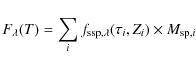
3 The spectral energy distribution of a NB-TSPH simulation: S PECODY
As already mentioned, owing to the mass resolution of the dynamical
simulations fixed by the number of particles to our disposal, each
star-particle has the mass ![]() or so (see Table 2),
i.e. each star-particle represents a big assembly of real
stars which distribute in mass according to a given initial mass
function and are all born in a short burst of star formation, therefore
being homogeneous both in age and chemical composition.
In this way, each star-particle can be approximated to a SSP
of mass
or so (see Table 2),
i.e. each star-particle represents a big assembly of real
stars which distribute in mass according to a given initial mass
function and are all born in a short burst of star formation, therefore
being homogeneous both in age and chemical composition.
In this way, each star-particle can be approximated to a SSP
of mass
![]() .
.
To derive the SED of our NB-TSPH galaxy model we start from
the definition of the integrated monochromatic flux generated by the
stellar content of a galaxy of age T
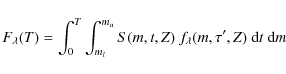
|
(1) |
where S(m,t,Z) denotes the stellar birth-rate and
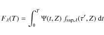
|
(2) |
where
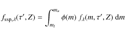
|
(3) |
is defined as the integrated monochromatic flux of a SSP, i.e. of a coeval, chemically homogeneous assembly of stars with age
where
![\begin{figure}
\par\includegraphics[width=12cm,clip]{12709fig4.eps}
\end{figure}](/articles/aa/full_html/2010/10/aa12709-09/img93.png)
|
Figure 4:
SEDs of the model galaxies for the different cosmological scenarios,
shown at different ages as indicated ( |
| Open with DEXTER | |
3.1 Some details on the SSPs in use
In this paper we have adopted the SSPs computed by Tantalo (2005) and available online from the Padova Galaxies and Single Stellar Population Models database (GALADRIEL) at http://www.astro.unipd.it/galadriel/.
The spectral energy distributions (SEDs) of the SSPs have been calculated following the method described by Bressan et al. (1994). To this purpose we have adopted the stellar tracks calculated by Girardi et al. (2000). These stellar models include modern physical input as far as opacity, nuclear reaction rates, neutrino losses, mixing schemes, etc. are concerned. The evolutionary sequences go from the zero age main sequence to the latest evolutionary phases and cover wide ranges of stellar masses and chemical compositions. In particular, they include the planetary nebula phase, the so-called AGB manqué phase that may develop in low-mass stars when the metallicity is higher than about three times solar, and the extended horizontal branch typical of low-mass stars with very low metallicity. Finally, the underlying isochrones are calculated by means of the algorithm of ``equivalent evolutionary points'' described in Bertelli et al. (1994).
In order to derive SEDs, magnitudes, and colors, corresponding to a source of given luminosity, effective temperature, gravity, and chemical composition, one needs a library of stellar spectra as function of these parameters. The spectral library considered in this paper was assembled by Girardi et al. (2002) adopting the ATLAS9 release (Kurucz 1993) of synthetic atmospheres: these latter are those for the no-overshooting case calculated by Castelli et al. (1997) and subsequently extended by other authors.
For each SSP, GALADRIEL provides also large tabulations of magnitudes and colors for the following photometric systems:
- Bessell-Brett.
- Hubble Space Telescope (NICMOS, WFPC2, ACS).
- Sloan Digital Sky Survey (SDSS).
- GAIA.
- GALEX.
In this study we have considered only two photometric systems:
the Bessell-Brett and SDSS for the VEGAmag and ABmag. The transmission
curves considered for first photometric system are from
Bessell (1990) for the ![]() passbands
and from Bessell & Brett
(1988) for the
passbands
and from Bessell & Brett
(1988) for the ![]() passbands.
The SDSS photometric system (Fukugita
et al. 1996) comprises five non-overlapping
passbands that range from the ultraviolet cutoff
at 3000 Å to the sensitivity limit of silicon CCDs at
11 000 Å. To interpret large samples of
galaxies of recent acquisition, such as COSMOS and GOODS, we
have also implemented the photometric systems used in these campaigns
(see below).
passbands.
The SDSS photometric system (Fukugita
et al. 1996) comprises five non-overlapping
passbands that range from the ultraviolet cutoff
at 3000 Å to the sensitivity limit of silicon CCDs at
11 000 Å. To interpret large samples of
galaxies of recent acquisition, such as COSMOS and GOODS, we
have also implemented the photometric systems used in these campaigns
(see below).
3.2 SEDs of the galaxy models
Using the above technique and integrating over the SEDs of all star-particles we can derive the SEDs of the model galaxies. The SEDs are shown in Fig. 4 at different ages (in view of the cosmological application of these results we remind the reader that these are the SEDs seen in the rest-frame).
It is worth noting that starting from the age of about
5 Gyr the three SEDs show an important ultraviolet excess,
i.e. rising branch and a peak in the flux short-ward
of 2000 Å. At the last age in common,
7 Gyr, the flux level is nearly comparable in the ![]() and
and ![]() models and
significantly lower in the
models and
significantly lower in the ![]() case.
For the two models arriving to 13 Gyr age,
namely
case.
For the two models arriving to 13 Gyr age,
namely ![]() and
and ![]() ,
the ultraviolet excess in the first model is significantly
higher than in the second one. What is the source of this excess of
flux? There are several candidates: the short-lived planetary
nebulae, the AGB manqué phase for stars with the appropriate
metallicity, the hot horizontal branch stars of low metal content, and
finally massive stars if star formation is going on. The Planetary
Nebulae are the descendants of low- and intermediate-mass stars on
their way from AGB to the White Dwarf regime. Although they can be very
bright and hot, they are too short-lived (a few 104 yr).
The AGB manqué stars have a low-mass and a lifetime amounting
to a fraction of the core He-burning phase. These stars appear when the
age is older than approximately 5-6 Gyr. Low-mass stars of
very low metal content during part of their core He-burning phase in a
very extended horizontal branch are bright and long lived so that they
may significantly contribute to the UV flux. Finally there are
the young stars if star formation goes on even at minimal levels of
activity. Owing to the much higher intrinsic luminosity of these
stars, if they are present even in small numbers they would
significantly contribute to the flux in the far ultraviolet.
Disentangling the contribution of each possible source is a cumbersome
affair. The fact that the flux in this wavelength interval increases
starting from about 5 Gyr suggests a combination of
AGB manqué stars and young stars, leaving planetary nebulae
and extreme horizontal branch objects in the background.
,
the ultraviolet excess in the first model is significantly
higher than in the second one. What is the source of this excess of
flux? There are several candidates: the short-lived planetary
nebulae, the AGB manqué phase for stars with the appropriate
metallicity, the hot horizontal branch stars of low metal content, and
finally massive stars if star formation is going on. The Planetary
Nebulae are the descendants of low- and intermediate-mass stars on
their way from AGB to the White Dwarf regime. Although they can be very
bright and hot, they are too short-lived (a few 104 yr).
The AGB manqué stars have a low-mass and a lifetime amounting
to a fraction of the core He-burning phase. These stars appear when the
age is older than approximately 5-6 Gyr. Low-mass stars of
very low metal content during part of their core He-burning phase in a
very extended horizontal branch are bright and long lived so that they
may significantly contribute to the UV flux. Finally there are
the young stars if star formation goes on even at minimal levels of
activity. Owing to the much higher intrinsic luminosity of these
stars, if they are present even in small numbers they would
significantly contribute to the flux in the far ultraviolet.
Disentangling the contribution of each possible source is a cumbersome
affair. The fact that the flux in this wavelength interval increases
starting from about 5 Gyr suggests a combination of
AGB manqué stars and young stars, leaving planetary nebulae
and extreme horizontal branch objects in the background.
3.3 Magnitudes and colors of galaxy models
Given a photometric system, it is straightforward to derive the temporal evolution of magnitudes and colors of each star-particle and of the whole galaxy. For the sake of illustration we show results only for the Bessell-Brett and the SDSS photometric systems.
Star-particle by star-particle view.
In Fig. 5 we show the color evolution of the![\begin{figure}
\par\includegraphics[width=6cm,clip]{12709fig5a.eps}\hspace*{1mm}...
...2.6cm}\includegraphics[width=13cm]{12709fig5e.eps}\hspace*{2.6cm}}\end{figure}](/articles/aa/full_html/2010/10/aa12709-09/img97.png)
|
Figure 5:
Three-dimensional view of the |
| Open with DEXTER | |
Integrated magnitudes and colors.
The evolution of the integrated magnitudes in the rest-frame, for the![\begin{figure}
\par\includegraphics[width=8.0cm,height=8cm]{12709fig6a.eps}\includegraphics[width=8.0cm,height=8cm]{12709fig6b.eps}
\end{figure}](/articles/aa/full_html/2010/10/aa12709-09/img98.png)
|
Figure 6:
Left panel: rest-frame evolution of the total
absolute Bessell & Brett magnitudes, MK,
MV, MB,
and M1550, of the |
| Open with DEXTER | |
The temporal evolution of magnitudes mirrors the history of star formation (see Fig. 1): in brief the magnitudes decrease as the galaxy gets the peak of SFR and hence becomes more luminous. Afterwards, the magnitudes increase following the SFR that declines rapidly. Figure 6 shows the magnitudes MB, MV, MK, and M1550 of the SCDM case for the Bessell-Brett system (left panel). The 1550-magnitude, that probes the UV region of the spectrum, weights the star formation at each epoch and reproduces the trend seen in the SFR. In the right panel of Fig. 6 we show the magnitudes in the SDSS photometric system of the same model. Although to lower extent, the same effect is visible in the u and g bands where the evolution is less smooth than for the other three bands.
![\begin{figure}
\par\includegraphics[width=8.0cm,height=8cm]{12709fig7a.eps}\hspace*{1mm}
\includegraphics[width=8.0cm,height=8cm]{12709fig7b.eps}
\end{figure}](/articles/aa/full_html/2010/10/aa12709-09/img99.png)
|
Figure 7:
Left panel: rest-frame evolution of the B-V,
V-K, and 1550-V colors
for the Bessell-Brett photometric system shown by our model galaxies as
indicated. Right panel: the same as in
the left panel but for SDSS colors u-r,
r-i, and r-z.
In both panels the |
| Open with DEXTER | |
![\begin{figure}
\par\includegraphics[width=17cm]{12709fig8.eps}
\end{figure}](/articles/aa/full_html/2010/10/aa12709-09/img100.png)
|
Figure 8:
Validation of the integrated colors of our models compared to the
observational data for a sample of nearby galaxies. We show the
color-color distribution of a sample of galaxies from
DR7 SDSS. The data are selected for |
| Open with DEXTER | |
The temporal evolution of colors is shown in the two panels of
Fig. 7.
Once again, the differences between models are primarily due to their
SFH. In brief, the
![]() and
and ![]() models
have the same prescription for the SFR; therefore they have similar
SFHs (both qualitatively and quantitatively) and similar color
evolution. In the
models
have the same prescription for the SFR; therefore they have similar
SFHs (both qualitatively and quantitatively) and similar color
evolution. In the ![]() case
with the multi-phase ISM, star formation is more gradual and lasts
longer, the peak of activity is lowered and shifted to older ages as
compared to the
case
with the multi-phase ISM, star formation is more gradual and lasts
longer, the peak of activity is lowered and shifted to older ages as
compared to the ![]() case.
The total mass assembled by the models is almost equal and the
different behavior obtained with the two star formation prescriptions
is likely due to the different time scales required to form new stars
(see Merlin & Chiosi 2007,
for details).
case.
The total mass assembled by the models is almost equal and the
different behavior obtained with the two star formation prescriptions
is likely due to the different time scales required to form new stars
(see Merlin & Chiosi 2007,
for details).
To assess the quality of the integrated colors of our models
we compare them to observed colors of a sample of nearby galaxies taken
from the SDSS-DR7 database. We select the sample with the following
criteria: the galaxies must have redshift ![]() ,
the galaxy images should be taken far away from the
CCD edges, they should unsaturated, and finally,
the photometric errors in each bands should be smaller than
0.1 mag (good signal to noise ratios). With these criteria we
obtain a sample of 5986 galaxies. Figure 8 shows the galaxies
in a color-color diagram and compare them with the rest-frame color
evolution of the models. The age increases as indicated by the arrow.
Galaxies classified as ETGs, using the exponential (
,
the galaxy images should be taken far away from the
CCD edges, they should unsaturated, and finally,
the photometric errors in each bands should be smaller than
0.1 mag (good signal to noise ratios). With these criteria we
obtain a sample of 5986 galaxies. Figure 8 shows the galaxies
in a color-color diagram and compare them with the rest-frame color
evolution of the models. The age increases as indicated by the arrow.
Galaxies classified as ETGs, using the exponential (
![]() )
and de Vaucouleurs' (
)
and de Vaucouleurs' (
![]() ) profile likelihoods
(see Shimasaku
et al. 2001; Strateva et al. 2001,
for more details on the SDSS morphological
classification), are indicated with empty circles, whereas late type
galaxies (LTGs) are shown with black dots. The sample has been
corrected for the extinction. The color evolution of our simulations is
indicated with filled squares, empty
circles, and filled triangles for the
three models. Remarkably, simulated colors and data nicely agree,
in particular for ages older than 5 Gyr.
) profile likelihoods
(see Shimasaku
et al. 2001; Strateva et al. 2001,
for more details on the SDSS morphological
classification), are indicated with empty circles, whereas late type
galaxies (LTGs) are shown with black dots. The sample has been
corrected for the extinction. The color evolution of our simulations is
indicated with filled squares, empty
circles, and filled triangles for the
three models. Remarkably, simulated colors and data nicely agree,
in particular for ages older than 5 Gyr.
3.4 Distribution of the stellar populations in the color-magnitude diagram
![\begin{figure}
\par\includegraphics[width=8.0cm,height=8.0cm]{12709fig9a.eps}\includegraphics[width=8.0cm,height=8.0cm]{12709fig9b.eps}
\end{figure}](/articles/aa/full_html/2010/10/aa12709-09/img104.png)
|
Figure 9:
Left panel: distribution of the stellar
populations in the (V-K)-V plane
for the |
| Open with DEXTER | |
It might be worth of interest to explore the age-metallicity range spanned by the stellar populations of a galaxy by looking at their distribution in the color-magnitude diagram (CMD), in analogy to what currently made for stars in clusters and fields.
![\begin{figure}
\par\includegraphics[width=18cm,clip]{12709fig10.eps}
\end{figure}](/articles/aa/full_html/2010/10/aa12709-09/img105.png)
|
Figure 10:
Distribution of the stellar populations in the (g-i) vs.
g plane for the |
| Open with DEXTER | |
![\begin{figure}
\par\includegraphics[width=18cm,clip]{12709fig11.eps}
\end{figure}](/articles/aa/full_html/2010/10/aa12709-09/img106.png)
|
Figure 11: Same as Fig. 10 but for stellar populations with different metallicity. As expected the stars of very low metallicity are in general very old, whereas at increasing metallicity stars of any age are possible. |
| Open with DEXTER | |
![\begin{figure}
\par\includegraphics[width=18cm,clip]{12709fig12.eps}
\end{figure}](/articles/aa/full_html/2010/10/aa12709-09/img107.png)
|
Figure 12: Same as Fig. 10 but for stars of any age and metallicity but different locations in the galaxy. |
| Open with DEXTER | |
The CMDs of Fig. 9 show SSPs of different age and metallicity, and the star-particles of the galaxy simulations (the filled circles). To calculate the magnitude of the SSPs we have assigned them the same mass of the star-particles in the NB-TSPH simulations. The solid lines show the evolutionary path followed by SSPs of different metal content as their integrated luminosity and color change as a function of the age. Along each line the age goes from 0.1 Gyr to 14 Gyr. This is the analog of the evolutionary path followed by stars of given mass and chemical composition. The dashed lines show SSPs of the same age (as indicated) and different metallicity. Along each line the metallicity goes from Z=0.0001 to Z=0.07. The CMDs allow us to catch immediately how the stellar populations of a model galaxy (as represented by its star-particles) distribute in age and metallicity. The analog of this situation for real stars would be a CMD built up with the integrated magnitudes and colors of the stellar clusters of a galaxy, for instance the clusters of the LMC and SMC, the only difference is that while real clusters have different mass our star-particles are all with the same mass. However, this is a point of minor relevance here.
In the (V-K) vs.
V diagram we can see how star-particles
distribute at varying the metallicity: in the ![]() galaxy at the age of
13 Gyr the vast majority of star-particles are very old. The
bulk of stars distribute along the lines of very old ages and span all
the values of metallicity. This means that the (V-K) color
tests the metallicities differences, more than the age. However there
is a fraction of younger stars that tends to crowd the region comprised
between Z=0.019 (
galaxy at the age of
13 Gyr the vast majority of star-particles are very old. The
bulk of stars distribute along the lines of very old ages and span all
the values of metallicity. This means that the (V-K) color
tests the metallicities differences, more than the age. However there
is a fraction of younger stars that tends to crowd the region comprised
between Z=0.019 (![]() )
and Z=0.070 (3.5
)
and Z=0.070 (3.5 ![]() ).
).
In the (1550-V) vs. V diagram, on the other hand, the bulk of the stars distribute along the Z=0.019 line and have ages going from very old to very young. Since the metallicity has a lower effect, this diagram can be used to infer the gross age of the stellar content of a galaxy.
To get a deeper insight of the whole problem, in
Figs. 10,
from left to right, we show the distribution of the stellar populations
in the g-(g-i) plane
for the ![]() model
at the age of 13 Gyr. In each panel, stars
younger than a certain limit (that varies from panel to panel as
indicated) are plotted as light dots, the remaining ones as
dark dots. The insert in the upper right corner in each panel shows the
position on the xy projection plane of
such stars (the light and dark dots). As expected,
owing to the residual star formation activity (say after the first
5 Gyr) stars of younger and younger age tend to concentrate
toward the galactic center. Keeping the same color-code,
in Fig. 11,
we show how the stars of different age distribute in metallicity.
As expected the stars of very low metallicity are in general
very old, whereas at increasing
metallicity stars of any age are possible. Finally,
in Fig. 12
we show how stars of different age and metallicity spatially distribute
within the galactic volume.
model
at the age of 13 Gyr. In each panel, stars
younger than a certain limit (that varies from panel to panel as
indicated) are plotted as light dots, the remaining ones as
dark dots. The insert in the upper right corner in each panel shows the
position on the xy projection plane of
such stars (the light and dark dots). As expected,
owing to the residual star formation activity (say after the first
5 Gyr) stars of younger and younger age tend to concentrate
toward the galactic center. Keeping the same color-code,
in Fig. 11,
we show how the stars of different age distribute in metallicity.
As expected the stars of very low metallicity are in general
very old, whereas at increasing
metallicity stars of any age are possible. Finally,
in Fig. 12
we show how stars of different age and metallicity spatially distribute
within the galactic volume.
![\begin{figure}
\par\includegraphics[width=8cm,height=8cm]{12709fig13.eps}
\end{figure}](/articles/aa/full_html/2010/10/aa12709-09/img109.png)
|
Figure 13:
Integrated (U-B)0
and (B-V)0 colors
of the LMC clusters by Bica
et al. (1991), open rhombs; the galactic
globular clusters by Harris (1996),
asterisks; the SSPs with different metallicity, dotted-dashed lines,
the heavy solid line is the one with the metallicity typical of the
LMC, i.e. Z=0.008); finally, the
star-particles of the |
| Open with DEXTER | |
In order to validate the quality of our photometry, we compare the
colors of our SSPs and star-particles of the NB-TSPH simulation with
the colors of observed real stellar clusters. This is shown in
Fig. 13,
where we display: the integrated (U-B)0
and (B-V)0 colors
of the LMC clusters by Bica
et al. (1991) (open rhombs); the Galactic Globular
Clusters by Harris (1996)
limited to a few indicative cases (asterisks); the SSPs with different
metallicity indicated by the dotted dashed lines (the heavy solid line
is for Z=0.008, the typical mean
metallicity of the LMC); finally the star-particles of the ![]() galaxy
model (small open circles). Data
and theoretical predictions seem to agree each other but for the
youngest clusters of the LMC which tend to scatter above the line for Z=0.008.
However, this is less of a problem as a plausible explanation has been
advanced by Girardi et al.
(1995). Therefore, the above agreement between theory and
data secures that our photometry is carefully calculated.
galaxy
model (small open circles). Data
and theoretical predictions seem to agree each other but for the
youngest clusters of the LMC which tend to scatter above the line for Z=0.008.
However, this is less of a problem as a plausible explanation has been
advanced by Girardi et al.
(1995). Therefore, the above agreement between theory and
data secures that our photometry is carefully calculated.
4 Cosmological spectro-photometric evolution: theory and data
The advent of the modern giant telescopes has opened a new era in observational cosmology and galaxy evolution can be traced back to very early stages. In this context, deep multi-color imaging surveys provide a powerful tool to access the population of faint galaxies with relatively high efficiency. These surveys span the whole spectral range from the UV to the near-IR bands, enabling galaxy evolution to be followed on a wide range of redshifts. Therefore it is worth looking at the cosmological evolution of our model galaxies and compare it with modern data. Since galaxies are observed at different redshifts in an expanding Universe, we need the so-called K-correction and E-corrections that can be easily derived together with magnitudes and colors from the population synthesis technique (see Rocca-Volmerange & Guiderdoni 1988; Bressan et al. 1994; Guiderdoni & Rocca-Volmerange 1987,1988). Finally, we compared the colors of our models with those of two sample of ETGs extracted from the COSMOS and GOODS databases.
![\begin{figure}
\par\includegraphics[width=8.0cm,height=8.0cm]{12709fig14.eps}
\end{figure}](/articles/aa/full_html/2010/10/aa12709-09/img110.png)
|
Figure 14: Red-shifted spectra at different redshifts for the three galaxy models. Internal extinction is taken into account. |
| Open with DEXTER | |
4.1 Evolutionary and cosmological corrections
When we consider a source observed at redshift z,
we need to remember that a photon observed at a wavelength
![]() has been emitted at wavelength
has been emitted at wavelength
![]() .
The two wavelengths are related by
.
The two wavelengths are related by
| (5) |
A source with apparent magnitude m measured in a photometric passband, is related to the absolute magnitude M, in the emission-frame passband, through the cosmological correction,
where DM is the distance modulus, defined by
![\begin{displaymath}%
DM =5 \log_{10}\left[ \frac{D_{L}(z)}{10~{\rm pc}} \right],
\end{displaymath}](/articles/aa/full_html/2010/10/aa12709-09/img116.png)
|
(7) |
being DL(z) the luminosity distance.
The above luminosity distance has been calculated with the
same cosmology of the simulated galaxies (
![]() ,
,
![]() , h0).
In particular, we have adopted the following equation (see Weinberg 1972;
Hogg 1999;
Kolb &
Turner 2000, for all details):
, h0).
In particular, we have adopted the following equation (see Weinberg 1972;
Hogg 1999;
Kolb &
Turner 2000, for all details):
![\begin{displaymath}%
D_{L}(z)= \frac{c}{H_{0}}(1+z)\int_{0}^{z}\frac{{\rm d}z}
{...
...{\rm M}(1+z)^{3} + \Omega_{\Lambda} \bigg]^{\frac{1}{2}}}\cdot
\end{displaymath}](/articles/aa/full_html/2010/10/aa12709-09/img117.png)
|
(8) |
If the source is at redshift z, then its luminosity is related to its spectral density flux (energy per unit time, unit area, and unit wavelength) by
|
(9) |
where
Finally, the ![]() in Eq. (6)
is
in Eq. (6)
is
![\begin{displaymath}%
K_{\rm corr} = 2.5 \log_{10} (1+z) + 2.5 \log_{10}
\left[ \frac{L(\lambda_{0})}{L(\lambda_{\rm e})} \right]
\end{displaymath}](/articles/aa/full_html/2010/10/aa12709-09/img120.png)
|
(10) |
(see the definition by Oke & Sandage 1968). This means that to make a fair comparison between objects at different redshifts, we must derive the rest-frame photometric properties of our observed galaxies (magnitudes, colors, etc.) by applying K-corrections.
In addition, we must also correct these rest-frame quantities for the
expected evolutionary changes over the redshift range studied,
by applying the so called evolutionary corrections,
![]() .
The
.
The
![]() are usually derived assuming a model for the galaxy SED and calculating
its evolution with the redshift. In this way we can recover the
evolution of the absolute magnitudes and colors as a function of the
redshift z, including the effect of the K-
and E-corrections on the SED of
our models.
are usually derived assuming a model for the galaxy SED and calculating
its evolution with the redshift. In this way we can recover the
evolution of the absolute magnitudes and colors as a function of the
redshift z, including the effect of the K-
and E-corrections on the SED of
our models.
Following Guiderdoni
& Rocca-Volmerange (1987), the cosmological K(z)
and evolutionary E(z) corrections
are conventionally given in terms of magnitude differences:
| K(z) = M(z,t0) - M(0,t0), | (11) |
| E(z) = M(z,tz) - M(z,t0), | (12) |
where M(0,t0) is the absolute magnitude in a passband derived from the rest frame spectrum of the galaxy at the current time, M(z,t0) is the absolute magnitude derived from the spectrum of the galaxy at the current time but red-shifted at z, and M(z,tz) is the absolute magnitude obtained from the spectrum of the galaxy at time tz and red-shifted at z.
From Eq. (6)
the apparent magnitude, in some broad-band filter and at
redshift z, is given by:
| m(z) = M(z) + E(z) + K(z) + DM(z). | (13) |
Obviously, the relation t=t(z), between the cosmic time t and the redshift z of a stellar population formed at a given redshift zf, depends on the cosmology considered and the parameters adopted. Following Kolb & Turner (2000):
![\begin{displaymath}%
t(z)= \frac{1}{H_{0}}\int_{z}^{\infty}\frac{{\rm d}z}{(1+z)...
...{\rm M}(1+z)^{3} + \Omega_{\Lambda} \bigg]^{\frac{1}{2}}}\cdot
\end{displaymath}](/articles/aa/full_html/2010/10/aa12709-09/img122.png)
|
(14) |
4.2 Extinction
Before calculating the ![]() ,
it is worth applying to the theoretical SEDs the effect of extinction
of the stellar luminosity caused by the presence of a certain amount of
metal-rich gas so that the SEDs get closer to the real ones. Although
the task is a complicate issue requiring a careful analysis (Piovan
et al. 2006a,2003,2006b), for the
purposes of the present study, the effect of extinction can be
evaluated using the relation proposed long ago by Guiderdoni & Rocca-Volmerange
(1987):
,
it is worth applying to the theoretical SEDs the effect of extinction
of the stellar luminosity caused by the presence of a certain amount of
metal-rich gas so that the SEDs get closer to the real ones. Although
the task is a complicate issue requiring a careful analysis (Piovan
et al. 2006a,2003,2006b), for the
purposes of the present study, the effect of extinction can be
evaluated using the relation proposed long ago by Guiderdoni & Rocca-Volmerange
(1987):
![\begin{displaymath}%
\tau_{\lambda} = 3.25(1-\omega_{\lambda})^{0.5}
(A_{\lambda}/A_{V})_{\odot} [Z(t)/Z_{\odot}]^{1.35} G(t),
\end{displaymath}](/articles/aa/full_html/2010/10/aa12709-09/img123.png)
|
(15) |
where
The monochromatic flux of the galaxy with the inclusion of the
effect due to extinction,
![]() ,
can be expressed in function of the monochromatic flux of the
rest-frame SED of the model galaxy
,
can be expressed in function of the monochromatic flux of the
rest-frame SED of the model galaxy
![]() (see Eq. (4)):
(see Eq. (4)):
where the right-hand part of the expression takes into account the transmission function for an angle of inclination i; we adopt here i=45. Although this relation was originally derived for disk galaxies, it can be safely used also in our case.
![\begin{figure}
\par\includegraphics[width=8.0cm,height=8.0cm]{12709fig15.eps}
\end{figure}](/articles/aa/full_html/2010/10/aa12709-09/img130.png)
|
Figure 15:
Top panels: comparison between the SEDs of
the |
| Open with DEXTER | |
The effect of extinction is included in our SEDs using Z(t)
and G(t) obtained from
the NB-TSPH simulations. Internal extinction may significantly redden
the colors, the effect being particularly
important on the color-redshift relation. To illustrate the
point, in Fig. 15
we compare the SEDs of the ![]() and
and ![]() models at the age of 13 Gyr with and without extinction,
as indicated. First of all the two SEDs are different even
neglecting extinction (they reach indeed different levels of flux),
see the top panels of Fig. 15. This simply
reflects the final lower mass in stars of the
models at the age of 13 Gyr with and without extinction,
as indicated. First of all the two SEDs are different even
neglecting extinction (they reach indeed different levels of flux),
see the top panels of Fig. 15. This simply
reflects the final lower mass in stars of the ![]() model
with respect to
model
with respect to ![]() (a factor of three lower). Second, the effect of extinction is
different in the two models (top panels of Fig. 15). This simply
reflects the different metallicity and gas content at the age of
13 Gyr. These are Z(t)=
0.0214 and G(t)=0.257
in
(a factor of three lower). Second, the effect of extinction is
different in the two models (top panels of Fig. 15). This simply
reflects the different metallicity and gas content at the age of
13 Gyr. These are Z(t)=
0.0214 and G(t)=0.257
in ![]() and Z(t)=0.0513
and
G(t)=0.441
in
and Z(t)=0.0513
and
G(t)=0.441
in ![]() .
The factor
.
The factor ![]() of Eq. (16)
with
of Eq. (16)
with ![]() is shown in the bottom
panel of Fig. 15.
is shown in the bottom
panel of Fig. 15.
There is a final point to consider, i.e. the
intrinsic reliability of the magnitudes and colors derived from SEDs as
a function of the redshift. To illustrate the point, in
Fig. 14
we display the red-shifted spectrum with extinction of the models for
some values of z. The spectra show a
drastic change in the slope that occurs at a certain wavelength whose
value increases with the redshift. This effect is because the
rest-frame theoretical spectra have a lower limit
of 912 Å and that the extension to ![]() < 912 Å
has been made by simply assuming
black-body spectra. The real spectrum short-ward of 912 Å
could be different from a pure black-body. The effect of this
approximation should be taken into account in the computation of the
colors in any photometric system. In other words, magnitudes and colors
that contain flux originated in the
< 912 Å
has been made by simply assuming
black-body spectra. The real spectrum short-ward of 912 Å
could be different from a pure black-body. The effect of this
approximation should be taken into account in the computation of the
colors in any photometric system. In other words, magnitudes and colors
that contain flux originated in the ![]() < 912 Å
interval become more and more uncertain at increasing redshift. This is
illustrated in Fig. 16
which displays the quantity
< 912 Å
interval become more and more uncertain at increasing redshift. This is
illustrated in Fig. 16
which displays the quantity ![]() .
The shaded area shows the region of intrinsic uncertainty due to the
above effect. It emerges from this that at redshift of z=3
(observational data in the surveys considered reach
this redshift) magnitudes are considered accurate at wavelengths
.
The shaded area shows the region of intrinsic uncertainty due to the
above effect. It emerges from this that at redshift of z=3
(observational data in the surveys considered reach
this redshift) magnitudes are considered accurate at wavelengths ![]() > 4100 Å.
> 4100 Å.
![\begin{figure}
\par\includegraphics[width=8cm,clip]{12709fig16.eps}
\end{figure}](/articles/aa/full_html/2010/10/aa12709-09/img134.png)
|
Figure 16:
Reliability of magnitudes and colors as function of the redshift is
because the theoretical spectra in the population synthesis algorithm
do not extend at wavelengths shorter than |
| Open with DEXTER | |
4.3 Comparison with data
The advent of large-scale space and ground-based surveys in a wide range of wavelengths is giving us unprecedented access to statistically large populations of galaxies at different redshifts (and also environments). The practical use of these immense databases requires some caution as far as galaxy detections, redshift assignment, galaxy classification, and galaxy selection are concerned. Prior to anything else it is worth recalling that owing to the enormous amounts of data to handle, the data acquisition process is usually made following automatic procedures that deserve some remarks.
Detection.
At z>5, traditional optical bands, e.g. UBVR, fall below the rest-frame wavelength that corresponds to the Lyman-break spectral feature (1216 Å), where most of the stellar radiation is extinguished by interstellar or intergalactic hydrogen. Because of this, galaxies at z>5 are practically invisible at those photometric bands, and even if they were detected, their colors would provide very little information about their stellar population. The color selection technique, e.g. the UGR selection of Lyman-Break Galaxy (LBGs) by Steidel et al. (1999,1996) and Steidel et al. (2003), has been used in some surveys to identify galaxies at high redshift, dramatically improving the efficiency of spectroscopic surveys at z>3.Redshift assignment.
Photometric redshifts are the logical extension of color selection by estimating redshifts and SEDs from many photometric bands. Unlike color selection, photometric redshifts take advantage of all available information, enabling redshift estimates along with the age, star formation rate and mass.Morphological classification.
One of the main characteristics of deep photometric surveys is the richness of detected objects, where a significant fraction of them appear as point sources that cannot be neither easily distinguished from real stars nor morphologically classified. Therefore, the classification by means of morphological and photometric criteria is a crucial issue. In this paper, we consider two deep catalogues that allow us to select good samples of ETGs.Selection.
Morphological selection of ETGs can be made using automated pipelines that isolate objects on the basis of their two-dimensional light distributions: this is the case of the COSMOS survey (see below). On the other hand, in the case of GOODS, it is possible to select more accurately these objects by correlating a catalogue of photometric and spectroscopic redshifts with a morphological one.4.4 COSMOS survey
In this analysis, we use the Cosmic Evolution Survey - COSMOS
official photometric redshift catalogue (Scoville
et al. 2007), designed to probe the evolution of
galaxies in the context of their large scale structure out to moderate
redshift. Details of the COSMOS catalogue are described in Capak et al. (2007) and Mobasher et al. (2007).
It covers a 2 square degree area with deep
panchromatic data and includes objects whose total i magnitudes
(i+ or ![]() )
are brighter than 25.
)
are brighter than 25.
The COSMOS multi-band catalogue embraces data from different
telescopes, as listed in Table 4, and presents
imaging data and photometry that cover various photometric bands
between 0.3 ![]() and 2.4
and 2.4 ![]() .
The catalogue was generated using SExtractor (Bertin
& Arnouts 1996) and contains photometry measured over
3 arcsec diameter apertures for all the bands. All magnitudes
are in the AB system. The cosmology adopted is: H0=70 km s-1 Mpc-1,
.
The catalogue was generated using SExtractor (Bertin
& Arnouts 1996) and contains photometry measured over
3 arcsec diameter apertures for all the bands. All magnitudes
are in the AB system. The cosmology adopted is: H0=70 km s-1 Mpc-1,
![]() and
and ![]() .
It also contains photometric redshifts, 68 and
95 percent confidence intervals, and spectral types calculated
with two different packages: the Mobasher
et al. (2007) and the Bayesian Photometric Redshift
(BPZ by Benítez 2000).
.
It also contains photometric redshifts, 68 and
95 percent confidence intervals, and spectral types calculated
with two different packages: the Mobasher
et al. (2007) and the Bayesian Photometric Redshift
(BPZ by Benítez 2000).
Such a large database needs an automated and objective
morphological classification procedure separating ETGs from other
objects. The goal is achieved using the parameter
![]() ,
which is based on the spectral type. Objects with
,
which is based on the spectral type. Objects with ![]() correspond to ETGs, those with
correspond to ETGs, those with ![]() to all the remaining types.
to all the remaining types.
Table 4: COSMOS survey: telescopes and optical/IR bands.
![\begin{figure}
\par\includegraphics[width=8cm,height=8cm]{12709fig17.eps}
\end{figure}](/articles/aa/full_html/2010/10/aa12709-09/img143.png)
|
Figure 17:
Cosmological evolution with redshift for the (
BJ-r+) color
of the COSMOS survey. Both passbands are those of the Subaru Telescope.
All galaxies of the catalog are shown in light stars. The ETGs selected
with the pipeline morphological |
| Open with DEXTER | |
![\begin{figure}
\par\includegraphics[width=8cm,height=8cm]{12709fig18.eps}
\end{figure}](/articles/aa/full_html/2010/10/aa12709-09/img144.png)
|
Figure 18:
Same as Fig. 17
but for the (
|
| Open with DEXTER | |
![\begin{figure}
\par\includegraphics[width=8cm,height=8cm]{12709fig19.eps}
\end{figure}](/articles/aa/full_html/2010/10/aa12709-09/img145.png)
|
Figure 19: Same as Fig. 17 but for the (g-r) color (SDSS survey passbands). |
| Open with DEXTER | |
Table 5: GOODS database: telescopes and optical/IR bands.
For our model galaxies we generate magnitudes and colors in
the same photometric system of COSMOS, and calculate the cosmological
and evolutionary corrections suited to the cosmological background
in use. Colors and their cosmological evolution in different bands are
shown in Figs. 17-19, where the BJ-r+ (Subaru),
![]() (Subaru/KPNO), and
the g-r (SDSS) colors
are plotted as an example. It is worth calling attention that
the model
(Subaru/KPNO), and
the g-r (SDSS) colors
are plotted as an example. It is worth calling attention that
the model
![]() is plotted from
is plotted from
![]() down to
down to ![]() because it has been stopped at the age of 7 Gyr.
For the sake of comparison, first we display all the galaxies
from the survey, independently of their classification (light stars)
and, superposed to them, we mark in dark stars the sub-sample of ETGs
selected following the classification suggested by the automated
pipeline
(
because it has been stopped at the age of 7 Gyr.
For the sake of comparison, first we display all the galaxies
from the survey, independently of their classification (light stars)
and, superposed to them, we mark in dark stars the sub-sample of ETGs
selected following the classification suggested by the automated
pipeline
(
![]() ).
The photometric evolution for our three model galaxies is also shown:
the solid line is for the
).
The photometric evolution for our three model galaxies is also shown:
the solid line is for the ![]() ,
the dotted-dashed line is for the
,
the dotted-dashed line is for the ![]() CDM model, and the
dotted line is for the
CDM model, and the
dotted line is for the ![]() case.
case.
The models follow the general trend of the observations and,
in particular, are marginally consistent with the group of
ellipticals up to ![]() beyond which the data are too poor to say anything. The observed
ellipticals are indeed redder than the mean value of the data and
theoretical predictions. Concerning the theoretical values, their bluer
colors can be ascribed to the tail of star formation extending to the
present. Although this minor stellar activity does not
significantly affect the gross features of the models (structure, mass
distributions etc.) it certainly affect the colors
making them bluer than desired and expected. This secondary star
formation activity is likely a spurious effect (work is progress to
cope with this). Another point of uncertainty could reside in the
selection criteria to identify ETGs.
beyond which the data are too poor to say anything. The observed
ellipticals are indeed redder than the mean value of the data and
theoretical predictions. Concerning the theoretical values, their bluer
colors can be ascribed to the tail of star formation extending to the
present. Although this minor stellar activity does not
significantly affect the gross features of the models (structure, mass
distributions etc.) it certainly affect the colors
making them bluer than desired and expected. This secondary star
formation activity is likely a spurious effect (work is progress to
cope with this). Another point of uncertainty could reside in the
selection criteria to identify ETGs.
4.5 GOODS database
For the sake of comparison, we consider now the Great Observatories Origins Deep Survey - GOODS database (Giavalisco et al. 2004). The survey is based on the observations of two separate fields centered on the Hubble Deep Field North (HDFN) and Chandra Deep Field South (CDFS) and includes ultra-deep images from ACS on HST, from mid-IR satellite Spitzer, as well as from a number of ground-based facilities (see Table 5).
Galaxies exhibit a range of morphologies that are difficult to
determine automatically, so a manual classification
is often used to test the efficacy of automated classifiers. For this
reason, in order to select ETGs from the database we have
cross-correlated two catalogues: the GOODS - Multi-wavelength
Southern Infrared Catalogue (GOODS-MUSIC) by Grazian
et al. (2006) to determine the redshift and the one
by Bundy et al. (2005)
to fix the morphology. These are good catalogues to rely on.
The first one indeed contains redshifts of high precision.
In fact the GOODS-MUSIC database (Grazian
et al. 2006) comprises photometric and spectroscopic
information for galaxies in the GOODS Southern Field. For these objects
they find excellent agreement between photometric and spectroscopic
redshifts over the range 0<z<6 (see
Fig. 12
in Grazian et al. 2006,
for the ![]() relation).
relation).
In the second one, Bundy
et al. (2005) present a morphological catalogue of
galaxies in the GOODS North and South Fields, for which the
morphological classification has been made by hand, therefore more
being reliable than the one derived from automated procedure. The study
relies on the combination of many different data sets in the GOODS
fields including infrared observations as listed in Table 5, spectroscopic
and photometric redshifts, and HST morphologies. The catalogue
contains objects with a magnitude limit based on HST-ACS imaging data
released by the GOODS team
(Giavalisco et al. 2004).
A z-band selected catalogue was constructed
running SExtractor (Bertin &
Arnouts 1996) and considering a magnitude limit of ![]() ,
where reliable visual morphological classification was deemed possible.
All magnitudes are defined in the ABmag system and they assume
a cosmology with
,
where reliable visual morphological classification was deemed possible.
All magnitudes are defined in the ABmag system and they assume
a cosmology with ![]() ,
,
![]() ,
and H0=70. The resulting
sample of objects over both GOODS fields was inspected visually by Bundy et al. (2005) who
classified each one of them, by using the technique discussed in Brinchmann & Ellis (2000),
according to a scale that separates stars from compact objects and
galaxies of different morphological type.
,
and H0=70. The resulting
sample of objects over both GOODS fields was inspected visually by Bundy et al. (2005) who
classified each one of them, by using the technique discussed in Brinchmann & Ellis (2000),
according to a scale that separates stars from compact objects and
galaxies of different morphological type.
We cross-correlated the two catalogues described above to recover a data set of galaxies with reliable morphological classification and precise redshift determination. Therefore these samples of galaxies should be considered much better selected than the sample derived from COSMOS. Standing on those arguments, a final sub-sample of ETGs is selected from the complete database. The total amounts to 118 objects.
![\begin{figure}
\par\includegraphics[width=8cm,height=8cm]{12709fig20.eps}
\end{figure}](/articles/aa/full_html/2010/10/aa12709-09/img152.png)
|
Figure 20:
Cosmological evolution with redshift of the V(F606W)-i(F775W) colors
of the GOODS survey (ACS-HST passbands) for early-type galaxies with
spectroscopic (empty circle) and photometric (filled circles) redshift
determination as indicated. The galaxy models for the
three different cosmological scenarios are shown superimposed to the
data, continuous and dotted lines as labelled. The |
| Open with DEXTER | |
![\begin{figure}
\par\includegraphics[width=8cm,height=8cm]{12709fig21.eps}
\end{figure}](/articles/aa/full_html/2010/10/aa12709-09/img153.png)
|
Figure 21: Same as Fig. 20 but for the V(F606W)-z(F850LP) colors (ACS-HST passbands). |
| Open with DEXTER | |
![\begin{figure}
\par\includegraphics[width=8cm,height=8cm]{12709fig22.eps}
\end{figure}](/articles/aa/full_html/2010/10/aa12709-09/img154.png)
|
Figure 22:
Same as Fig. 20
but for the |
| Open with DEXTER | |
In Figs. 20-22, the (
V(F606W)-i(F775W)),
(
V(F606W)-z(F850LP)),
and
(
![]() ) colors
of this selected sample are shown together with the theoretical
predictions. The same remark on the redshift spanned by the
model
) colors
of this selected sample are shown together with the theoretical
predictions. The same remark on the redshift spanned by the
model
![]() made above applies also here. For all of the colors,
the agreement between data and theory concerning the
photometric, cosmological evolution with redshift is remarkably good.
Furthermore, the theoretical colors seem to match the
GOODS data much better than COSMOS values.
made above applies also here. For all of the colors,
the agreement between data and theory concerning the
photometric, cosmological evolution with redshift is remarkably good.
Furthermore, the theoretical colors seem to match the
GOODS data much better than COSMOS values.
This clearly shows that the reliability of the morphology classifier plays an important role in these matters. The selection in GOODS is made by correlating two catalogues, one containing photometric and spectroscopic redshifts, the other listing galaxies with good morphological classification (made by hand). In contrast, in COSMOS classification and selection are fully automated with no any cross-correlation with other criteria.
Another possible explanation for the differences between the results from COSMOS and GOODS, could be an intrinsic difference in the samples of observed galaxies. First, the COSMOS database has a lower magnitude limit that makes the morphological classification more difficult. Second, two different packages are used to calculate the redshift with a mean dispersion of 0.0315. Finally, there are some problems with the using the SExtractor (Bertin & Arnouts 1996) star/galaxy separator parameter that is not stable with a variable seeing. All this goes in favor of the GOODS database of ETGs.
5 Surface photometry of ETGs
Surface photometry is one of the most powerful tools to study the properties and history of ETGs. The analysis is based on fitting ellipses to the isophotes of a galaxy. The oldest fit of the radial intensity profile is the empirical de Vaucouleurs law (de Vaucouleurs 1948) that has now been extended by the more flexible Sérsic profile (Sérsic 1968). The derived properties, of which the most important ones are the intensity distribution, the radial ellipticity, and the position angle profiles, provide basic information such as effective radius, deviations from the ellipses, isophote twisting, triaxiality, and absolute magnitudes. The associated higher order Fourier coefficients from the fits reveal the intrinsic ``boxy'' or ``disky'' appearance of the isophotes which can be used to uncover the underlying stellar components.
In this section we will show how, starting from a 3D numerical simulation of a galaxy, we can recover ``artificial'' images projected on a plane, from which photometric and structural parameters, such as luminosity, magnitudes, colors, and effective radius, can be calculated. These images are analyzed as if they were realistic images of galaxies taken with a telescope. In this way we can derive morphological and structural parameters of the models that can be compared with those of real ETGs. In particular we derive the Kormendy relation (the projection of the Fundamental Plane on the luminosity-radius plane). Finally, we make use of the SDSS photometric system.
For the aims of this analysis, we did not include the effects of extinction. This can be justified as follows. The artificial images we are using refer to the present epoch, when SFR has dropped by orders of magnitudes with respect to the past and the galaxies are nearly passively evolving. Furthermore, as a consequence of galactic winds, all interstellar gas and dust have been expelled from the central regions of galaxies. The issue has been discussed in some detail by Galletta et al. (2007) who made use of the same galaxy models and to whom we refer. In brief, to investigate the spectro-photometric evolution of the NB-TSPH models by Merlin & Chiosi (2006,2007), Galletta et al. (2007) studied the relative spatial distribution of stars and gas and found that while most of the stars are located inside about half viral radius, most of the gas falls outside. This implies that effects of dust (extinction) become important only in the very outer regions of ETGs. Of course, a completely different situation is expected to occur at high redshifts, when the evolutionary stage reached by a galaxy is such that most of gas is likely to fall in the innermost regions whereby star formation is still active. In such a case, the effects of extinctions cannot be neglected. In any case, work is in progress to include extinction in the SEDs of simulations as observed along a given line of sight, by considering the geometrical structure of the galaxies.
![\begin{figure}
\par\mbox{\includegraphics[width=5cm,height=5cm]{12709fig23a.ps}\...
...ncludegraphics[width=5cm,height=1cm]{12709fig23d.ps}\hspace*{5cm}}\end{figure}](/articles/aa/full_html/2010/10/aa12709-09/img155.png)
|
Figure 23:
r-band artificial image of a 80 |
| Open with DEXTER | |
5.1 Artificial images
Starting from the 3D NB-TSPH simulations, we construct 2D images projecting the volume with |z| < 100 kpc onto the xy plane. The information we need are the spatial coordinates of the star-particles and their SEDs. With these projections on a plane we construct discrete grids at the nodes of which we calculate the total flux given by all the particles along the line of sight. These fluxes feed the photometric code to compute the magnitude and/or color in a given band for each mesh point of the grid. The flux of each star-particle of given age and metallicity is the one of the associated SSPs. Therefore there is full consistency between the SEDs of the star particles and those required by the photometric code in use.
To create good artificial images, the grids must be large enough to encompass all the star-particles of the model galaxy, and must contain a large enough number of grid points to eventually get smooth images. A scale length of 80-100 kpc is long enough to include all the star-particles of our simulations and a grid with 100-200 points along each direction is good enough to secure smooth images; the best combination to obtain satisfactory results is a scale of 0.4 to 0.8 kpc per grid point and direction. Table 6 gives the resolution under which images have been created: the choice of the scale depends on the model galaxy and its diameter.
Table 6: Construction of artificial images: dimensions and grid scales.
Images are built up for the last computed stage of the model
galaxies at the ages listed in Table 3. Figure 23 shows the
2D distribution of the star-particles of the models as traced
by the star-particle r-magnitudes of the
SDSS system. A grid of 200 ![]() 200 mesh points is used to span a square region of
80 kpc side. In all the models, the old
star-particles appear to be spatially distributed mimicking the
morphology of an elliptical galaxy. The left panel refers to the
200 mesh points is used to span a square region of
80 kpc side. In all the models, the old
star-particles appear to be spatially distributed mimicking the
morphology of an elliptical galaxy. The left panel refers to the ![]() model,
the middle to the
model,
the middle to the
![]() ,
and the right to the
,
and the right to the ![]() .
In displaying these frames the intensity contrast between the
bright central regions and the low surface brightness of the outer
parts is very difficult to portray
using a linear relation, so that the logarithmic scale is more
convenient. It is worth noting that the inclination of the
major axis of the projected distribution with respect to the coordinate
axes
simply reflect the spatial distribution of the star-particles in the
3D space and in the 2D projection. No other
physical meaning in involved.
.
In displaying these frames the intensity contrast between the
bright central regions and the low surface brightness of the outer
parts is very difficult to portray
using a linear relation, so that the logarithmic scale is more
convenient. It is worth noting that the inclination of the
major axis of the projected distribution with respect to the coordinate
axes
simply reflect the spatial distribution of the star-particles in the
3D space and in the 2D projection. No other
physical meaning in involved.
5.2 Isophotal analysis
The images used in this section are similar to those of Fig. 23 but are based on
a grid of 100 ![]() 100 mesh points (enough to describe a square region of
80 kpc side). These images are analysed with the IRAF
packages Stsdas.Isophot (designed to deal with
elliptical isophotes) and Ellipse (designed to
derive the brightness distribution of a galaxy).
100 mesh points (enough to describe a square region of
80 kpc side). These images are analysed with the IRAF
packages Stsdas.Isophot (designed to deal with
elliptical isophotes) and Ellipse (designed to
derive the brightness distribution of a galaxy).
Stsdas.Isophot (using all the data of the galaxy image) extracts the intensity levels, which are nicely fitted by ellipses, and determines the center, the ellipticity, the position angle, and the length of the semi-major axis. However, small but significant deviations from pure ellipses are also present. For each isophote, these deviations are measured along the contour and are recovered by the Fourier analysis on the distance of the ellipsoidal contour as a function of the azimuthal angle.
Ellipse fits the elliptical isophotes and
measures the isophotal parameters of a galaxy's image in whatsoever
passband (SDSS in our case). The parameters are determined for each
isophote. The algorithm follows the method described by Jedrzejewski (1987).
In brief, assumed a provisional guess for an isophote's center
coordinates (
![]() ),
ellipticity (
),
ellipticity (![]() )
and semi-major axis position angle (
)
and semi-major axis position angle (![]() ), at each point along the semi-major
axis, the intensity
), at each point along the semi-major
axis, the intensity ![]() of the image is azimuthally sampled along an elliptical path.
of the image is azimuthally sampled along an elliptical path. ![]() is
then expanded into a Fourier series as
is
then expanded into a Fourier series as
![\begin{displaymath}%
I(\phi) = I_0 + \sum_k[A_{k}{\rm sin}(k\phi) + B_{k}{\rm cos}(k\phi)].
\end{displaymath}](/articles/aa/full_html/2010/10/aa12709-09/img160.png)
|
(17) |
A best fit procedure (minimization of the sum of the squares of the residuals between the real distribution of data and an elliptical one) fixes the parameters
| (18) |
The amplitudes A1, B1, A2, B2 give information on how much the estimated intensity profile deviates from the real one, so they give the errors in the fitting procedure. The image data is fitted by the function
where the amplitudes A3, B3, A4, B4 measure the isophote's deviations from perfect ellipticity.
Higher order moments (![]() )
define deviations of the isophotes from ellipses. In practice,
moments beyond the fourth cannot be measured accurately; third and
fourth-order moments are calculated from the equation above by fixing
the first and second-order moments to their best-fit values. The
third-order moments (A3
and B3) represent
isophotes with three-fold deviations from ellipses
(e.g., egg-shaped or heart-shaped) while the fourth-order
moments (A4
and B4) represent
four-fold deviations. Rhomboidal or diamond-shaped isophotes translate
into a non-zero A4.
For galaxies which are not distorted by interactions, B4 is
the most meaningful moment: a positive B4
indicates ``disky'' isophotes (i.e., with semi-major axis B4
)
define deviations of the isophotes from ellipses. In practice,
moments beyond the fourth cannot be measured accurately; third and
fourth-order moments are calculated from the equation above by fixing
the first and second-order moments to their best-fit values. The
third-order moments (A3
and B3) represent
isophotes with three-fold deviations from ellipses
(e.g., egg-shaped or heart-shaped) while the fourth-order
moments (A4
and B4) represent
four-fold deviations. Rhomboidal or diamond-shaped isophotes translate
into a non-zero A4.
For galaxies which are not distorted by interactions, B4 is
the most meaningful moment: a positive B4
indicates ``disky'' isophotes (i.e., with semi-major axis B4 ![]() 100 percent longer than the best fitting ellipse), whereas a
negative B4
indicates ``boxy'' isophotes (i.e., with semi-major axis B4
100 percent longer than the best fitting ellipse), whereas a
negative B4
indicates ``boxy'' isophotes (i.e., with semi-major axis B4 ![]() 100 percent
shorter than the best fitting ellipse Jedrzejewski
1987).
100 percent
shorter than the best fitting ellipse Jedrzejewski
1987).
When running Ellipse on model galaxies, we adopt the following guidelines. The length of the semi-major axis is increased on a logarithmic scale (10% longer in our case). With a new semi-major axis, a new isophote is calculated using the best-fit parameters obtained from the previous isophote. In general, all the parameters can vary freely, even though the routine may fail to converge on isophotes with large deviations from ellipses. In such cases to achieve convergence it is necessary to fix the value of one or more parameters. The isophotal center is not let wander around by more than 2 grid points between consecutive isophotes; in practice the center is found to be rather stable.
Given the isophotal center and the semi-major axis, at any
position a along the semi-major axis we
determine the radius,
![]() ,
of a circle corresponding to the local
ellipse as
,
of a circle corresponding to the local
ellipse as
where
After using the ellipse task to measure the mean radial intensity profiles and fit ellipses to the image, the program Bimodel is used to reconstruct a model image from the results of isophotal analysis. Bimodel creates a 2D smooth image of the source image. In Fig. 24 are shown the smooth images of the three simulations corresponding to the discrete images of Fig. 23 with the elliptical isophotes overlapped. The same remark made for the inclination of the semi-major axis with respect to the X-axis in Fig. 23 applies also here.
The ![]() and
and ![]() harmonics
from the photometry are added to the model. This option is most useful
when working close to the central intensity peak. As explained
in Jedrzejewski (1987), the
sampling at small radii may introduce a ``boxy'' component. More
accurate modelling of the central region is generally achieved when
including this component.
harmonics
from the photometry are added to the model. This option is most useful
when working close to the central intensity peak. As explained
in Jedrzejewski (1987), the
sampling at small radii may introduce a ``boxy'' component. More
accurate modelling of the central region is generally achieved when
including this component.
![\begin{figure}
\par\includegraphics[width=8cm]{12709fig24a.ps}\par\includegraphi...
...8cm]{12709fig24b.ps}\par\includegraphics[width=8cm]{12709fig24c.ps}
\end{figure}](/articles/aa/full_html/2010/10/aa12709-09/img172.png)
|
Figure 24:
Two-dimensional models of the optical r-band
magnitude in the xy-plane of the images shown in
Fig. 23.
Superposed are elliptical isophotes (white solid lines). The
top panel is for |
| Open with DEXTER | |
5.3 Parametrization of the intensity profile
The intensity I(R) and
corresponding surface brightness ![]() are given by the Sérsic laws
are given by the Sérsic laws
![\begin{displaymath}%
I(R) = I_{\rm e}\exp \left\{ -b_{n} \biggl[ \biggl( \frac{R}{R_{\rm e}}
\biggl)^{1/n} - 1 \biggr] \right\},
\end{displaymath}](/articles/aa/full_html/2010/10/aa12709-09/img174.png)
|
(21) |
![\begin{displaymath}%
\mu(R) = \mu_{\rm e} - 2.5b_{n} \biggl[ \biggl( \frac{R}{R_{\rm e}}
\biggl)^{1/n} - 1 \biggl] \log e,
\end{displaymath}](/articles/aa/full_html/2010/10/aa12709-09/img175.png)
|
(22) |
where r is the radius from the center in kpc,
For a Sérsic model with ![]() ,
the effective radius
,
the effective radius ![]() contains roughly half the integrated light if bn=2n-0.324
(Trujillo et al. 2001).
The parameter n controls the overall shape
of a Sérsic profile, with low n values
producing curved profiles with logarithmic slopes which are shallow in
the inner regions, and steep in the outer parts, while high n values
produce
extended profiles with less overall curvature.
contains roughly half the integrated light if bn=2n-0.324
(Trujillo et al. 2001).
The parameter n controls the overall shape
of a Sérsic profile, with low n values
producing curved profiles with logarithmic slopes which are shallow in
the inner regions, and steep in the outer parts, while high n values
produce
extended profiles with less overall curvature.
By definition, the parameters are chosen in such a way that
the model reduces to the de Vaucouleurs law for n=4,
and the consistency with the usual interpretation of ![]() as the radius enclosing half-light is secured.
as the radius enclosing half-light is secured.
The Sérsic model offers significant advantages. First and foremost, it provides a good description of the inner (100 pc scale) profiles, and a significantly better description when the profiles are extended to the kpc-scale (Trujillo et al. 2004; Graham et al. 2003).
The intensity profile is derived using the nfit1d
algorithm which provides 1D, non-linear fits to the image
(chi-square minimization). As nfit1d
supports any analytical fitting function, given the initial guesses for
the function coefficients, we have obtained the intensity profile of
the model galaxy with a Sérsic law with suitable
index n, together with the effective
radius ![]() and the effective intensity
and the effective intensity ![]() .
Figure 25
shows the best fitting Sérsic function for the r-band
in the particular sample. The profile inside the central
region whose radius is equal to 1-2 times the softening length
(1-2 kpc in our case), is excluded from the fit as it
is likely to be influenced by force softening. To derive the
effective radius, we reach large enough distances such as
15-20 kpc. The solid curve represents the best-fit Sérsic
model to the final profile (shown as solid symbols).
.
Figure 25
shows the best fitting Sérsic function for the r-band
in the particular sample. The profile inside the central
region whose radius is equal to 1-2 times the softening length
(1-2 kpc in our case), is excluded from the fit as it
is likely to be influenced by force softening. To derive the
effective radius, we reach large enough distances such as
15-20 kpc. The solid curve represents the best-fit Sérsic
model to the final profile (shown as solid symbols).
From the fitted intensity profiles and the best-fit
parameters, we calculate the effective radii ![]() and the total magnitudes in all bands for the three galaxy models. The
Sérsic index and
and the total magnitudes in all bands for the three galaxy models. The
Sérsic index and ![]() are listed in Table 7
for the various passbands.
are listed in Table 7
for the various passbands.
![\begin{figure}
\par\includegraphics[width=8.8cm]{12709fig25.eps}
\end{figure}](/articles/aa/full_html/2010/10/aa12709-09/img179.png)
|
Figure 25:
Intensity profiles fitted with a Sérsic law of variable index.
The r-band Sérsic index n
and the effective radius |
| Open with DEXTER | |
Table 7: Sérsic indexes and effective radii expressed in kpc for the SDSS photometric passbands and for all model galaxies.
The effective radius varies with the band from which is
derived, roughly decreasing as the band moves toward the shorter
wavelengths. Bernardi
et al. (2003a) finds that half-light angular sizes
of the
galaxies in their sample are indeed larger in the blue bands and they
show how the effective physical radii in their sample changes in the
four![]() bands. This trend is
followed by our simulations: the agreement is particularly
good for the
bands. This trend is
followed by our simulations: the agreement is particularly
good for the ![]() model.
For the other two, the trend is recovered only in the
bluer bands, whereas the radius increases again as the band shifts
toward longer wavelengths.
model.
For the other two, the trend is recovered only in the
bluer bands, whereas the radius increases again as the band shifts
toward longer wavelengths.
5.4 Structural properties
![\begin{figure}
\par\includegraphics[width=17cm,clip]{12709fig26.eps}
\end{figure}](/articles/aa/full_html/2010/10/aa12709-09/img180.png)
|
Figure 26:
Ellipticity |
| Open with DEXTER | |
In the various panels of Fig. 26 we show the
basic structural parameters of the three models. In brief, the
ellipticity ![]() (top panels), position angle PA (middle panels), and
deviation A4 of the
isophotes from pure ellipses (bottom panels) are shown as a function of
the ``geometric mean'' radius
(top panels), position angle PA (middle panels), and
deviation A4 of the
isophotes from pure ellipses (bottom panels) are shown as a function of
the ``geometric mean'' radius
![]() ,
as defined in Eq. (20)
for all the galaxy models as indicated. To the sake of
illustration, we show the results limited to the r-band
image.
,
as defined in Eq. (20)
for all the galaxy models as indicated. To the sake of
illustration, we show the results limited to the r-band
image.
Although the isophotes shown in Fig. 24 are well
approximated by ellipses, small but significant deviations from perfect
ellipsoidal shapes are measured. Of particular interest is
the A4 parameter![]() , which measures the
deviations from perfect ellipses: A4
< 0 corresponds to ``boxy'' isophotes, whereas A4
> 0 implies ``disky'' isophotes.
, which measures the
deviations from perfect ellipses: A4
< 0 corresponds to ``boxy'' isophotes, whereas A4
> 0 implies ``disky'' isophotes.
The radial profile of the A4
parameter indicates that the deviations from perfect ellipses are
generally negligibly small for the ![]() and
and ![]() models. In the case of the
models. In the case of the ![]() model,
the negative values of A4
in the outer regions tell us that there is a ``boxy'' structure.
model,
the negative values of A4
in the outer regions tell us that there is a ``boxy'' structure.
5.5 Color profiles
As mentioned before, Bernardi et al. (2003a) found that half-light angular sizes of the galaxies change in function of the band in which they are measured, finding larger radii with bluer bands. On average, the fact that ETGs have this trend implies that they present color gradients. It is known from observations that these gradients are such that ETGs are redder in their cores and bluer in the outskirts. This fact is thought to originate from variations in age or metallicity of the underlying stellar populations (Tantalo et al. 1998a; Worthey et al. 1994).
The radial color profiles of our models are shown in the three
panels of Fig. 27
which display the u-g, g-r,
r-i, and i-z color
profiles in the SDSS photometric system. With the physical
processes we have considered, colors are bluer in the
central cores and the color gradients are very small for the ![]() and
and ![]() models (left and
middle panels of Figs. 27).
In contrast, the central regions are
redder and the color gradients are significant for the
models (left and
middle panels of Figs. 27).
In contrast, the central regions are
redder and the color gradients are significant for the ![]() model
(right panel of Fig. 27).
Therefore, the typical color gradients of ETGs are not strictly
reproduced by our models, except for the
model
(right panel of Fig. 27).
Therefore, the typical color gradients of ETGs are not strictly
reproduced by our models, except for the ![]() case.
case.
The main reason for the central regions being bluer than
expected and observed resides in the prolonged stellar activity present
mainly in the central regions of all the models together with
insufficient increase of the mean metallicity in those regions.
To cast light on the effect of the long tail of star
formation, we have artificially stopped star formation at different
epochs. The details of these experiments are not shown here for the
sake of brevity. As expected, stopping star formations
immediately yields redder colors in the center, for instance
by about 0.1 mag in (B-V).
In addition, we have applied the cut in star formation to
star-particles enclosed within a given galacto-centric distance going
from 50 kpc to
![]() .
The result is that the effect on the color gets stronger moving
outward. In all cases, the color difference amounts to 0.1
to 0.2 mag
in the typical (B-V).
What we learn from this is that further investigation of other star
formation prescriptions and effects of feedback with better resolution
in the central regions is required.
.
The result is that the effect on the color gets stronger moving
outward. In all cases, the color difference amounts to 0.1
to 0.2 mag
in the typical (B-V).
What we learn from this is that further investigation of other star
formation prescriptions and effects of feedback with better resolution
in the central regions is required.
![\begin{figure}
\par\includegraphics[width=17.5cm,clip]{12709fig27.eps}
\end{figure}](/articles/aa/full_html/2010/10/aa12709-09/img182.png)
|
Figure 27:
Left panel: radial profiles of the |
| Open with DEXTER | |
6 Scaling laws: the Kormendy relation
As long known, ETGs are similar in their structural and dynamical properties and obey to empirically relationships among colors, luminosities, half-light radii, surface brightness profiles, and velocity dispersions that are ultimately related to their stellar content and dynamics. They are known as the Scaling Laws, among which particularly important are the Fundamental Plane and the Kormendy Relation.
Fundamental Plane (FP).
Long ago Djorgovski & Davis (1987) and Dressler et al. (1987) found that| (23) |
where
The existence of the FP has strong implications on galaxy formation and evolution theories. The small scatter in the FP (see e.g. Jorgensen et al. 1996) and its apparent lack of evolution with redshift (van Dokkum et al. 2000; Franx 1995; Bender 1996; van Dokkum & Franx 1996; Ellis et al. 1997), the homogeneity (Bower et al. 1992a), and the evidence for short (<1 Gyr) star formation timescales in these systems, all indicate that the bulk of stellar population in ETGs indeed formed at high redshift (z>2). Measuring the three parameters entering the FP for ETGs at varying redshift highlights some important questions concerning their age, formation history, and internal properties. One can answer questions such as how far in the past does the FP apply and whether its parameters evolved significantly with time. A study of the galaxy properties as a function of look-back time provides a good probe of the possible evolutionary differences. In this sense, we plan to study this scaling law at intermediate redshift by deriving its key parameters as function of time, i.e. considering the evolution with redshift of the ETGs.
In order to compare our models with real galaxies on
the FP, we need the theoretical central velocity
dispersion, ![]() .
Observationally, this is evaluated within an aperture
typically
less than about half the effective radius. Unfortunately, velocities
within such small radii in the simulations are significantly affected
by the softening parameter that in our case amounts
to 1 kpc. As accurate predictions
for
.
Observationally, this is evaluated within an aperture
typically
less than about half the effective radius. Unfortunately, velocities
within such small radii in the simulations are significantly affected
by the softening parameter that in our case amounts
to 1 kpc. As accurate predictions
for ![]() are not possible with our models, we have to leave aside the analysis
of the FP.
are not possible with our models, we have to leave aside the analysis
of the FP.
Kormendy Relation (KR).
Better chances are possible with this relation. The KR is the projection of the FP onto the luminosity-radius plane. It relates
|
(24) |
Many studies have confirmed that the luminous ETGs in clusters approximately follow the relation
The KR for galaxies in clusters at increasing redshift has
been claimed to be consistent with passively evolving stellar
populations (van
Dokkum et al. 1998; Ziegler & Bender 1997; van Dokkum
& Franx 1996; Aragon-Salamanca et al. 1993;
Bender
et al. 1998,1996; Bower et al. 1992b; Jorgensen
& Hjorth 1997).
On the other hand, some studies have also claimed that the data are
consistent with the hierarchical evolutionary scenario (White & Rees 1978). La Barbera et al. (2003),
working with cluster ETGs at
different redshift, found that the slope of the KR is almost invariant
up to ![]() with value of
with value of ![]()
![]() 0.08.
The homogeneity and the invariance with redshift of these
distributions is also suggested by the analysis of the
SDSS data by Bernardi
et al. (2003b).
0.08.
The homogeneity and the invariance with redshift of these
distributions is also suggested by the analysis of the
SDSS data by Bernardi
et al. (2003b).
To compare our models with observational data, we have chosen a sub-sample of ETGs from the Sloan Digital Sky Survey (SDSS; York et al. 2000; Stoughton et al. 2002) database. The SDSS survey has mapped one-quarter of the entire sky, producing a detailed image of it and determining the positions and photometric properties of more than 100 million celestial objects. The SDSS obtained high-resolution images in five different bands, namely u, g, r, i, and z (Fukugita et al. 1996), thus allowing for a reliable identification of ETGs and precise measurements of their photometric properties.
Galaxies can be selected using automated pipelines that
isolate objects on the basis of their 2D light distributions.
We consider ETGs from the DR2 release selected following the criteria
described in Bernardi
et al. (2003a) who have produced a catalogue of ![]() low-redshift
ETGs, selected using a combination of SDSS pipeline
parameters. This catalogue contains galaxies with a high i-band
concentration index (r50/r90)>2.5
and in which a de Vaucouleurs
(1948) fit to the surface brightness profile is significantly
more likely than an exponential fit. Details of the selection
can be found in Bernardi
et al. (2003a).
low-redshift
ETGs, selected using a combination of SDSS pipeline
parameters. This catalogue contains galaxies with a high i-band
concentration index (r50/r90)>2.5
and in which a de Vaucouleurs
(1948) fit to the surface brightness profile is significantly
more likely than an exponential fit. Details of the selection
can be found in Bernardi
et al. (2003a).
![\begin{figure}
\par\includegraphics[width=8.0cm,height=8.0cm]{12709fig28.eps}
\end{figure}](/articles/aa/full_html/2010/10/aa12709-09/img199.png)
|
Figure 28: Magnitude-radius relation in the r-band for the ETGs selected from the SDSS DR2 database following the criteria from Bernardi et al. (2003a). Results for our three model galaxies are shown for comparison. See the text for all details. |
| Open with DEXTER | |
In Fig. 28
we show the ![]() relation
found by Bernardi et al.
(2003c) for the sample of elliptical galaxies selected as
mentioned above. The luminosity-size relation for r-band
is
relation
found by Bernardi et al.
(2003c) for the sample of elliptical galaxies selected as
mentioned above. The luminosity-size relation for r-band
is ![]() .
For comparison, we show the results for our three model
galaxies. The
.
For comparison, we show the results for our three model
galaxies. The ![]() and Mr magnitude
within it of the models are:
and Mr magnitude
within it of the models are: ![]() = 5.42 kpc
and Mr =
-21.77 for the
= 5.42 kpc
and Mr =
-21.77 for the ![]() model;
model;
![]() =
2.7 kpc and Mr =
-22.02 for the
=
2.7 kpc and Mr =
-22.02 for the ![]() case;
case;
![]() =
3.27 and Mr =
-20.48 for the
=
3.27 and Mr =
-20.48 for the ![]() galaxy.
galaxy.
The ![]() and
and ![]() lie above the mean relation but fall in the data crowd. The
lie above the mean relation but fall in the data crowd. The ![]() model
falls below the mean line but still compatible with data.
No case lies close to the mean line. There are several reasons
to account for the marginal discrepancy. The discussion is slightly
different for the
model
falls below the mean line but still compatible with data.
No case lies close to the mean line. There are several reasons
to account for the marginal discrepancy. The discussion is slightly
different for the ![]() and
and ![]() models
evolved up to the age of 13 Gyr and the
models
evolved up to the age of 13 Gyr and the ![]() stopped at 7 Gyr.
stopped at 7 Gyr.
To bring the position of the ![]() and
and ![]() models down to the mean line one should increase the total star mass
and
models down to the mean line one should increase the total star mass
and ![]() by a factor of 1.5 or so. The solution is viable in
the sense that other models of the same type with better tuned
parameters could reach the
agreement. The same reasoning cannot be applied to the model
by a factor of 1.5 or so. The solution is viable in
the sense that other models of the same type with better tuned
parameters could reach the
agreement. The same reasoning cannot be applied to the model
![]() because its evolution terminated at 7 Gyr (
because its evolution terminated at 7 Gyr (![]() ). Looking
at the fading lines (magnitudes versus age) of Fig. 6 a shift of the Mr magnitude
of about +1 mag in 6 Gyr (to get the age
of 13 Gyr) is possible without changing the star
mass, thus bringing the model onto the mean line without
changing
). Looking
at the fading lines (magnitudes versus age) of Fig. 6 a shift of the Mr magnitude
of about +1 mag in 6 Gyr (to get the age
of 13 Gyr) is possible without changing the star
mass, thus bringing the model onto the mean line without
changing ![]() .
Most likely, an increase of
.
Most likely, an increase of ![]() of the same entity as in the previous cases is also possible. The arrow
in Fig. 28
shows the expected shift. Also in this case, agreement can be easily
achieved. To conclude, all the three models are marginally
consistent with the data. No better comparison is possible at
this stage.
of the same entity as in the previous cases is also possible. The arrow
in Fig. 28
shows the expected shift. Also in this case, agreement can be easily
achieved. To conclude, all the three models are marginally
consistent with the data. No better comparison is possible at
this stage.
7 General discussion and concluding remarks
We have presented a package of numerical codes to compute the spectroscopic and photometric properties of model galaxies by combining the evolutionary population synthesis technique with the 3D geometrical structure of the galaxy and its history of star formation and chemical enrichment, provided by NB-TSPH simulations. The tool is very flexible in the way input libraries of evolutionary tracks, isochrones, SSPs and important physical laws such as the initial mass function, star formation rate, and metallicity enrichment can be changed, tested, and added to the database for future use. Finally, it can be adapted to any photometric system currently in use. The method has been tested so far on three models of ETGs evolved within different cosmological backgrounds and the analysis has been done in the following photometric systems: Bessell-Brett, SDSS, COSMOS, and GOODS filters among all the ones we have at disposal. Our main results may be summarized as follows:
- 1.
- The application of the tool to three model galaxies at our
disposal, allow us to compute the SED, magnitudes, and colors as
function of time and redshift, together with the evolutionary and
cosmological corrections. With the aid of it, we analyzed
samples of ETGs taken from the COSMOS and GOODS databases, and made a
qualitative and quantitative comparison between theoretical results and
observational data. For both data-sets, we find that the simulated
colors for the different cosmological scenarios follow the general
trend over the entire range of redshift considered and are in good
agreement with the data up to ,
above which the number of observed ETGs falls abruptly.
In conclusion, within the redshift range considered, all the
simulated colors reproduce quite well the observational data.
- 2.
- We have also generated synthetic 2D images of the
galaxy models in a given photometric system. These synthetic images can
be processed with the same algorithms used to analyze real images
to derive the structural and morphological parameters,
e.g. the galaxy's
 and the luminosity within this, the shape indices through Fourier and
Sérsic analysis, the color profiles, and the radial profiles of most of
the parameters that define the structure of galaxies. We find that the
luminosity profiles of the model galaxies at z = 0
can be reasonably fitted with a Sérsic R1/n law.
The evaluation of the
in the photometric bands of SDSS shows the
same dependence on the passband wavelength range of the observational
data. Furthermore, the isophotes are well approximated by
ellipses, with only a weak radial variation in position angle and
ellipticity. Small but significant deviations from perfect ellipses are
also measured. In general, we can recover properties that
resemble those of observed galaxies.
and the luminosity within this, the shape indices through Fourier and
Sérsic analysis, the color profiles, and the radial profiles of most of
the parameters that define the structure of galaxies. We find that the
luminosity profiles of the model galaxies at z = 0
can be reasonably fitted with a Sérsic R1/n law.
The evaluation of the
in the photometric bands of SDSS shows the
same dependence on the passband wavelength range of the observational
data. Furthermore, the isophotes are well approximated by
ellipses, with only a weak radial variation in position angle and
ellipticity. Small but significant deviations from perfect ellipses are
also measured. In general, we can recover properties that
resemble those of observed galaxies.
- 3.
- In addition to that, we looked at the Kormendy relation, one of the Scaling Laws of ETGs, for which all theoretical counterparts of observational data were available. The theoretical luminosities and effective radii of the models are consistent with the archival data from the SDSS for a sample of ETGs.
We like to thank Dr. Mariangela Bernardi for kindly providing the data from the SDSS database.
References
- Aragon-Salamanca, A., Ellis, R. S., Couch, W. J., & Carter, D. 1993, MNRAS, 262, 764 [NASA ADS] [CrossRef] [Google Scholar]
- Arimoto, N., & Yoshii, Y. 1987, A&A, 173, 23 [NASA ADS] [Google Scholar]
- Barger, A. J., Cowie, L. L., Smail, I., et al. 1999, AJ, 117, 2656 [NASA ADS] [CrossRef] [Google Scholar]
- Barnes, J., & Hut, P. 1986, Nature, 324, 446 [NASA ADS] [CrossRef] [Google Scholar]
- Barnes, J. E., & Hernquist, L. 1996, ApJ, 471, 115 [NASA ADS] [CrossRef] [Google Scholar]
- Bell, E. F., Wolf, C., Meisenheimer, K., et al. 2004, ApJ, 608, 752 [NASA ADS] [CrossRef] [Google Scholar]
- Bender, R. 1997, in The Nature of Elliptical Galaxies, ed. M. Arnaboldi, G. S. Da Costa, & P. Saha, ASP Conf. Ser., 116, 11 [Google Scholar]
- Bender, R., Ziegler, B., & Bruzual, G. 1996, ApJ, 463, L51 [NASA ADS] [CrossRef] [Google Scholar]
- Bender, R., Saglia, R. P., Ziegler, B., et al. 1998, ApJ, 493, 529 [NASA ADS] [CrossRef] [Google Scholar]
- Benítez, N. 2000, ApJ, 536, 571 [NASA ADS] [CrossRef] [Google Scholar]
- Benz, W. 1990, in Numerical Modelling of Nonlinear Stellar Pulsations Problems and Prospects, ed. J. R. Buchler, 269 [Google Scholar]
- Berczik, P., Hensler, G., Theis, C., & Spurzem, R. 2003, Ap&SS, 284, 865 [NASA ADS] [CrossRef] [Google Scholar]
- Bernardi, M., Sheth, R. K., Annis, J., et al. 2003a, AJ, 125, 1817 [NASA ADS] [CrossRef] [Google Scholar]
- Bernardi, M., Sheth, R. K., Annis, J., et al. 2003b, AJ, 125, 1849 [NASA ADS] [CrossRef] [Google Scholar]
- Bernardi, M., Sheth, R. K., Annis, J., et al. 2003c, AJ, 125, 1866 [NASA ADS] [CrossRef] [Google Scholar]
- Bertelli, G., Bressan, A., Chiosi, C., Fagotto, F., & Nasi, E. 1994, A&AS, 106, 275 [NASA ADS] [Google Scholar]
- Bertin, E., & Arnouts, S. 1996, A&AS, 117, 393 [NASA ADS] [CrossRef] [EDP Sciences] [Google Scholar]
- Bessell, M. S. 1990, PASP, 102, 1181 [NASA ADS] [CrossRef] [Google Scholar]
- Bessell, M. S., & Brett, J. M. 1988, PASP, 100, 1134 [NASA ADS] [CrossRef] [Google Scholar]
- Bica, E., Barbuy, B., & Ortolani, S. 1991, ApJ, 382, L15 [NASA ADS] [CrossRef] [Google Scholar]
- Boissier, S., & Prantzos, N. 1999a, Ap&SS, 265, 409 [NASA ADS] [CrossRef] [Google Scholar]
- Boissier, S., & Prantzos, N. 1999b, MNRAS, 307, 857 [NASA ADS] [CrossRef] [Google Scholar]
- Bower, R. G., Lucey, J. R., & Ellis, R. S. 1992a, MNRAS, 254, 601 [NASA ADS] [CrossRef] [Google Scholar]
- Bower, R. G., Lucey, J. R., & Ellis, R. S. 1992b, MNRAS, 254, 589 [NASA ADS] [CrossRef] [Google Scholar]
- Bressan, A., Chiosi, C., & Fagotto, F. 1994, ApJS, 94, 63 [NASA ADS] [CrossRef] [Google Scholar]
- Brinchmann, J., & Ellis, R. S. 2000, ApJ, 536, L77 [NASA ADS] [CrossRef] [Google Scholar]
- Bundy, K., Ellis, R. S., & Conselice, C. J. 2005, ApJ, 625, 621 [NASA ADS] [CrossRef] [Google Scholar]
- Bundy, K., Ellis, R. S., Conselice, C. J., et al. 2006, ApJ, 651, 120 [NASA ADS] [CrossRef] [Google Scholar]
- Butcher, H., & Oemler, Jr., A. 1978, ApJ, 219, 18 [NASA ADS] [CrossRef] [Google Scholar]
- Capak, P., Aussel, H., Ajiki, M., et al. 2007, ApJS, 172, 99 [NASA ADS] [CrossRef] [Google Scholar]
- Cardelli, J. A., Clayton, G. C., & Mathis, J. S. 1989, ApJ, 345, 245 [NASA ADS] [CrossRef] [Google Scholar]
- Carraro, G., Lia, C., & Chiosi, C. 1998, MNRAS, 297, 1021 [NASA ADS] [CrossRef] [MathSciNet] [Google Scholar]
- Castelli, F., Gratton, R., & Kurucz, R. 1997, A&A, 318, 841 [NASA ADS] [Google Scholar]
- Chiosi, C. 2000, in Spectro-photometric Dating of Stars and Galaxies, ed. I. Hubney, S. R. Heap, & R. H. Cornett, ASP Conf. Ser, 192, 251 [Google Scholar]
- Chiosi, C., & Carraro, G. 2002, MNRAS, 335, 335 [NASA ADS] [CrossRef] [Google Scholar]
- Cimatti, A. 2009, in AIP Conf. Ser. 1111, ed. G. Giobbi, A. Tornambe, G. Raimondo, M. Limongi, L. A. Antonelli, N. Menci, & E. Brocato, 191 [Google Scholar]
- de Vaucouleurs, G. 1948, Ann. Astrophys., 11, 247 [Google Scholar]
- Djorgovski, S. G., & Davis, M. 1987, ApJ, 313, 59 [Google Scholar]
- Draine, B. T., & Lee, H. M. 1984, ApJ, 285, 89 [Google Scholar]
- Dressler, A. 1980, ApJ, 236, 351 [NASA ADS] [CrossRef] [Google Scholar]
- Dressler, A., Lynden-Bell, D., Burstein, D., et al. 1987, ApJ, 313, 42 [NASA ADS] [CrossRef] [Google Scholar]
- Eggen, O. J., Lynden-Bell, D., & Sandage, A. R. 1962, ApJ, 136, 748 [NASA ADS] [CrossRef] [Google Scholar]
- Ellis, R. S., Smail, I., Dressler, A., et al. 1997, ApJ, 483, 582 [NASA ADS] [CrossRef] [Google Scholar]
- Ferrini, F., & Poggianti, B. M. 1993, ApJ, 410, 44 [NASA ADS] [CrossRef] [Google Scholar]
- Fioc, M., & Rocca-Volmerange, B. 1997, A&A, 326, 950 [NASA ADS] [Google Scholar]
- Franx, M. 1995, in Stellar Populations, ed. P. C. van der Kruit, & G. Gilmore, IAU Symp., 164, 269 [Google Scholar]
- Fukugita, M., Hogan, C. J., & Peebles, P. J. E. 1998, ApJ, 503, 518 [NASA ADS] [CrossRef] [Google Scholar]
- Fukugita, M., Ichikawa, T., Doi, M., Shimasaku, K., & Schneider, D. 1996, AJ, 111, 1748 [NASA ADS] [CrossRef] [Google Scholar]
- Galletta, G., Casasola, V., Piovan, L., Merlin, E., & Bettoni, D. 2007, A&A, 462, 495 [NASA ADS] [CrossRef] [EDP Sciences] [Google Scholar]
- Giavalisco, M., Dickinson, M., Ferguson, H. C., et al. 2004, ApJ, 600, L103 [NASA ADS] [CrossRef] [Google Scholar]
- Gibson, B. K. 1997, MNRAS, 290, 471 [NASA ADS] [Google Scholar]
- Girardi, L., Chiosi, C., Bertelli, G., & Bressan, A. 1995, A&A, 298, 87 [NASA ADS] [Google Scholar]
- Girardi, L., Bressan, A., Bertelli, G., & Chiosi, C. 2000, A&AS, 141, 371 [Google Scholar]
- Girardi, L., Bertelli, G., Bressan, A., et al. 2002, A&A, 391, 195 [NASA ADS] [CrossRef] [EDP Sciences] [Google Scholar]
- Graham, A. W., Erwin, P., Trujillo, I., & Asensio Ramos, A. 2003, AJ, 125, 2951 [NASA ADS] [CrossRef] [Google Scholar]
- Grazian, A., Fontana, A., de Santis, C., et al. 2006, A&A, 449, 951 [NASA ADS] [CrossRef] [EDP Sciences] [Google Scholar]
- Guiderdoni, B., & Rocca-Volmerange, B. 1987, A&A, 186, 1 [NASA ADS] [Google Scholar]
- Guiderdoni, B., & Rocca-Volmerange, B. 1988, A&AS, 74, 185 [Google Scholar]
- Harris, W. E. 1996, AJ, 112, 1487 [NASA ADS] [CrossRef] [Google Scholar]
- Hogg, D. W. 1999 [arXiv:astro-ph/9812049], unpublished [Google Scholar]
- Hubble, E. 1936, ApJ, 84, 517 [NASA ADS] [CrossRef] [Google Scholar]
- Im, M., Griffiths, R. E., Ratnatunga, K. U., & Sarajedini, V. L. 1996, ApJ, 461, L79 [NASA ADS] [CrossRef] [Google Scholar]
- Immeli, A., Samland, M., Gerhard, O., & Westera, P. 2004, A&A, 413, 547 [NASA ADS] [CrossRef] [EDP Sciences] [Google Scholar]
- Jedrzejewski, R. I. 1987, MNRAS, 226, 747 [Google Scholar]
- Jorgensen, I., & Hjorth, J. 1997, in Galaxy Scaling Relations: Origins, Evolution and Applications, ed. L. N. da Costa, & A. Renzini, 175 [Google Scholar]
- Jorgensen, I., Franx, M., & Kjaergaard, P. 1996, MNRAS, 280, 167 [NASA ADS] [CrossRef] [Google Scholar]
- Kauffmann, G., White, S. D. M., & Guiderdoni, B. 1993, MNRAS, 264, 201 [NASA ADS] [CrossRef] [Google Scholar]
- Kobayashi, C. 2004a, Publications of the Astronomical Society of Australia, 21, 183 [NASA ADS] [CrossRef] [Google Scholar]
- Kobayashi, C. 2004b, MNRAS, 347, 740 [NASA ADS] [CrossRef] [Google Scholar]
- Kobayashi, C. 2005, MNRAS, 361, 1216 [NASA ADS] [CrossRef] [Google Scholar]
- Kodama, T., & Arimoto, N. 1997, A&A, 320, 41 [NASA ADS] [Google Scholar]
- Kolb, E. W., & Turner, M. S. 2000, Eur. Phys. J. C, 15, 125 [NASA ADS] [CrossRef] [EDP Sciences] [Google Scholar]
- Kurucz, R. 1993, in The Stellar Populations of Galaxies, ed. B. Barbuy, & A. Renzini (Dordrecht: Kluwer), IAU Symp., 149, 255 [Google Scholar]
- La Barbera, F., Busarello, G., Merluzzi, P., Massarotti, M., & Capaccioli, M. 2003, ApJ, 595, 127 [NASA ADS] [CrossRef] [Google Scholar]
- Larson, R. B. 1975, MNRAS, 173, 671 [NASA ADS] [CrossRef] [Google Scholar]
- Li, C., Jing, Y. P., Kauffmann, G., et al. 2006a, MNRAS, 368, 37 [NASA ADS] [Google Scholar]
- Li, C., Kauffmann, G., Jing, Y. P., et al. 2006b, MNRAS, 368, 21 [NASA ADS] [CrossRef] [Google Scholar]
- Li, C., Kauffmann, G., Wang, L., et al. 2006c, MNRAS, 373, 457 [NASA ADS] [CrossRef] [Google Scholar]
- Li, C., Jing, Y. P., Kauffmann, G., et al. 2007, MNRAS, 376, 984 [NASA ADS] [CrossRef] [Google Scholar]
- Lia, C., Portinari, L., & Carraro, G. 2002, MNRAS, 330, 821 [NASA ADS] [CrossRef] [Google Scholar]
- Lucy, L. B. 1977, AJ, 82, 1013 [NASA ADS] [CrossRef] [Google Scholar]
- Merlin, E., & Chiosi, C. 2006, A&A, 457, 437 [NASA ADS] [CrossRef] [EDP Sciences] [Google Scholar]
- Merlin, E., & Chiosi, C. 2007, A&A, 473, 733 [NASA ADS] [CrossRef] [EDP Sciences] [Google Scholar]
- Mobasher, B., Capak, P., Scoville, N. Z., et al. 2007, ApJS, 172, 117 [NASA ADS] [CrossRef] [Google Scholar]
- Oke, J. B., & Sandage, A. 1968, ApJ, 154, 21 [NASA ADS] [CrossRef] [Google Scholar]
- Patton, D. R., Pritchet, C. J., Yee, H. K. C., Ellingson, E., & Carlberg, R. G. 1997, ApJ, 475, 29 [NASA ADS] [CrossRef] [Google Scholar]
- Peebles, P. 2002, in A New Era in Cosmology, ASP Conf. Ser., 283, 351 [Google Scholar]
- Pérez-González, P. G., Rieke, G. H., et al. 2008, ApJ, 675, 234 [NASA ADS] [CrossRef] [Google Scholar]
- Piovan, L., Tantalo, R., & Chiosi, C. 2003, A&A, 408, 559 [NASA ADS] [CrossRef] [EDP Sciences] [Google Scholar]
- Piovan, L., Tantalo, R., & Chiosi, C. 2006a, MNRAS, 366, 923 [NASA ADS] [Google Scholar]
- Piovan, L., Tantalo, R., & Chiosi, C. 2006b, MNRAS, 370, 1454 [NASA ADS] [CrossRef] [Google Scholar]
- Pipino, A., & Matteucci, F. 2004, MNRAS, 347, 968 [NASA ADS] [CrossRef] [Google Scholar]
- Rocca-Volmerange, B., & Guiderdoni, B. 1988, A&AS, 75, 93 [Google Scholar]
- Samland, M. 2001, in Dynamics of Star Clusters and the Milky Way, ed. S. Deiters, B. Fuchs, A. Just, R. Spurzem, & R. Wielen, ASP Conf. Ser., 228, 559 [Google Scholar]
- Samland, M., & Gerhard, O. E. 2000, in Liege International Astrophysical Colloquia, ed. A. Noels, P. Magain, D. Caro, E. Jehin, G. Parmentier, & A. A. Thoul, 35, 415 [Google Scholar]
- Samland, M., Hensler, G., & Theis, C. 1997, ApJ, 476, 544 [NASA ADS] [CrossRef] [Google Scholar]
- Scannapieco, C., Tissera, P. B., White, S. D. M., & Springel, V. 2006a, MNRAS, 371, 1125 [NASA ADS] [CrossRef] [Google Scholar]
- Scannapieco, E., Kawata, D., Brook, C. B., et al. 2006b, ApJ, 653, 285 [NASA ADS] [CrossRef] [Google Scholar]
- Schade, D., Lilly, S. J., Crampton, D., et al. 1999, ApJ, 525, 31 [NASA ADS] [CrossRef] [Google Scholar]
- Scoville, N., Aussel, H., Benson, A., et al. 2007, ApJS, 172, 150 [Google Scholar]
- Searle, L., Sargent, W. L. W., & Bagnuolo, W. G. 1973, ApJ, 179, 427 [NASA ADS] [CrossRef] [Google Scholar]
- Sérsic, J. L. 1968, Atlas de galaxias australes, Cordoba, Argentina, Observatorio Astronomico [Google Scholar]
- Shimasaku, K., Fukugita, M., Doi, M., et al. 2001, AJ, 122, 1238 [NASA ADS] [CrossRef] [Google Scholar]
- Spergel, D. N., Verde, L., Peiris, H. V., et al. 2003, ApJS, 148, 175 [NASA ADS] [CrossRef] [Google Scholar]
- Steidel, C. C., Giavalisco, M., Dickinson, M., & Adelberger, K. L. 1996, AJ, 112, 352 [NASA ADS] [CrossRef] [Google Scholar]
- Steidel, C. C., Adelberger, K. L., Giavalisco, M., Dickinson, M., & Pettini, M. 1999, ApJ, 519, 1 [NASA ADS] [CrossRef] [Google Scholar]
- Steidel, C. C., Adelberger, K. L., Shapley, A. E., et al. 2003, ApJ, 592, 728 [NASA ADS] [CrossRef] [Google Scholar]
- Stoughton, C., Lupton, R. H., Bernardi, M., et al. 2002, AJ, 123, 485 [NASA ADS] [CrossRef] [Google Scholar]
- Strateva, I., Ivezic, Z., Knapp, G. R., et al. 2001, AJ, 122, 1861 [Google Scholar]
- Tantalo, R. 2005, in The Initial Mass Function 50 Years Later, ed. E. Corbelli, F. Palla, & H. Zinnecker, ASSL, 327, 235 [Google Scholar]
- Tantalo, R., Chiosi, C., Bressan, A., & Fagotto, F. 1996, A&A, 311, 361 [NASA ADS] [Google Scholar]
- Tantalo, R., Chiosi, C., & Bressan, A. 1998a, A&A, 333, 419 [NASA ADS] [Google Scholar]
- Tantalo, R., Chiosi, C., Bressan, A., Marigo, P., & Portinari, L. 1998b, A&A, 335, 823 [NASA ADS] [Google Scholar]
- Theis, C., Burkert, A., & Hensler, G. 1992, A&A, 265, 465 [NASA ADS] [Google Scholar]
- Treu, T., Ellis, R. S., Liao, T. X., et al. 2005, ApJ, 633, 174 [NASA ADS] [CrossRef] [Google Scholar]
- Trujillo, I., Graham, A. W., & Caon, N. 2001, MNRAS, 326, 869 [NASA ADS] [CrossRef] [Google Scholar]
- Trujillo, I., Erwin, P., Asensio Ramos, A., & Graham, A. W. 2004, AJ, 127, 1917 [NASA ADS] [CrossRef] [Google Scholar]
- van der Wel, A., Franx, M., van Dokkum, P. G., et al. 2005, ApJ, 631, 145 [NASA ADS] [CrossRef] [Google Scholar]
- van Dokkum, P. G., & Franx, M. 1996, MNRAS, 281, 985 [NASA ADS] [CrossRef] [Google Scholar]
- van Dokkum, P. G., Franx, M., Kelson, D. D., & Illingworth, G. D. 1998, ApJ, 504, L17 [NASA ADS] [CrossRef] [Google Scholar]
- van Dokkum, P. G., Franx, M., Fabricant, D., Illingworth, G. D., & Kelson, D. D. 2000, ApJ, 541, 95 [NASA ADS] [CrossRef] [Google Scholar]
- Vazdekis, A., Peletier, R. F., Beckman, J. E., & Casuso, E. 1997, ApJS, 111, 203 [NASA ADS] [CrossRef] [Google Scholar]
- Weinberg, S. 1972, Gravitation and Cosmology: Principles and Applications of the General Theory of Relativity [Google Scholar]
- White, S. D. M., & Rees, M. J. 1978, MNRAS, 183, 341 [NASA ADS] [CrossRef] [Google Scholar]
- Worthey, G., Faber, S. M., González, J. J., & Burstein, D. 1994, ApJS, 94, 687 [NASA ADS] [CrossRef] [Google Scholar]
- York, D. G., Adelman, J., Anderson, Jr., J. E., et al. 2000, AJ, 120, 1579 [Google Scholar]
- Ziegler, B. L., & Bender, R. 1997, MNRAS, 291, 527 [NASA ADS] [CrossRef] [Google Scholar]
Footnotes
- ... four
![[*]](/icons/foot_motif.png)
- They exclude the u-band as the measurements are affected by errors larger than the others.
- ... parameter
- A4 corresponds to the fourth order moment B4 of Eq. (19).
All Tables
Table 1: Cosmological parameters adopted in our simulations.
Table 2: Initial dynamical and computational parameters for the three model galaxies.
Table 3: End-product for the three model galaxies.
Table 4: COSMOS survey: telescopes and optical/IR bands.
Table 5: GOODS database: telescopes and optical/IR bands.
Table 6: Construction of artificial images: dimensions and grid scales.
Table 7: Sérsic indexes and effective radii expressed in kpc for the SDSS photometric passbands and for all model galaxies.
All Figures
|
|
Figure 1:
Star formation rate, in |
| Open with DEXTER | |
| In the text | |
|
|
Figure 2:
Growth of the fractionary total star mass
|
| Open with DEXTER | |
| In the text | |
|
|
Figure 3:
Left panel: mean metallicity Z(t)
versus time (in Gyr) for the three galaxy models, as
indicated. Right panel: metallicity distribution
(number of star-particles per metallicity bin) in the three models. The
histograms labelled |
| Open with DEXTER | |
| In the text | |
|
|
Figure 4:
SEDs of the model galaxies for the different cosmological scenarios,
shown at different ages as indicated ( |
| Open with DEXTER | |
| In the text | |
|
|
Figure 5:
Three-dimensional view of the |
| Open with DEXTER | |
| In the text | |
|
|
Figure 6:
Left panel: rest-frame evolution of the total
absolute Bessell & Brett magnitudes, MK,
MV, MB,
and M1550, of the |
| Open with DEXTER | |
| In the text | |
|
|
Figure 7:
Left panel: rest-frame evolution of the B-V,
V-K, and 1550-V colors
for the Bessell-Brett photometric system shown by our model galaxies as
indicated. Right panel: the same as in
the left panel but for SDSS colors u-r,
r-i, and r-z.
In both panels the |
| Open with DEXTER | |
| In the text | |
|
|
Figure 8:
Validation of the integrated colors of our models compared to the
observational data for a sample of nearby galaxies. We show the
color-color distribution of a sample of galaxies from
DR7 SDSS. The data are selected for |
| Open with DEXTER | |
| In the text | |
|
|
Figure 9:
Left panel: distribution of the stellar
populations in the (V-K)-V plane
for the |
| Open with DEXTER | |
| In the text | |
|
|
Figure 10:
Distribution of the stellar populations in the (g-i) vs.
g plane for the |
| Open with DEXTER | |
| In the text | |
|
|
Figure 11: Same as Fig. 10 but for stellar populations with different metallicity. As expected the stars of very low metallicity are in general very old, whereas at increasing metallicity stars of any age are possible. |
| Open with DEXTER | |
| In the text | |
|
|
Figure 12: Same as Fig. 10 but for stars of any age and metallicity but different locations in the galaxy. |
| Open with DEXTER | |
| In the text | |
|
|
Figure 13:
Integrated (U-B)0
and (B-V)0 colors
of the LMC clusters by Bica
et al. (1991), open rhombs; the galactic
globular clusters by Harris (1996),
asterisks; the SSPs with different metallicity, dotted-dashed lines,
the heavy solid line is the one with the metallicity typical of the
LMC, i.e. Z=0.008); finally, the
star-particles of the |
| Open with DEXTER | |
| In the text | |
|
|
Figure 14: Red-shifted spectra at different redshifts for the three galaxy models. Internal extinction is taken into account. |
| Open with DEXTER | |
| In the text | |
|
|
Figure 15:
Top panels: comparison between the SEDs of
the |
| Open with DEXTER | |
| In the text | |
|
|
Figure 16:
Reliability of magnitudes and colors as function of the redshift is
because the theoretical spectra in the population synthesis algorithm
do not extend at wavelengths shorter than |
| Open with DEXTER | |
| In the text | |
|
|
Figure 17:
Cosmological evolution with redshift for the (
BJ-r+) color
of the COSMOS survey. Both passbands are those of the Subaru Telescope.
All galaxies of the catalog are shown in light stars. The ETGs selected
with the pipeline morphological |
| Open with DEXTER | |
| In the text | |
|
|
Figure 18:
Same as Fig. 17
but for the (
|
| Open with DEXTER | |
| In the text | |
|
|
Figure 19: Same as Fig. 17 but for the (g-r) color (SDSS survey passbands). |
| Open with DEXTER | |
| In the text | |
|
|
Figure 20:
Cosmological evolution with redshift of the V(F606W)-i(F775W) colors
of the GOODS survey (ACS-HST passbands) for early-type galaxies with
spectroscopic (empty circle) and photometric (filled circles) redshift
determination as indicated. The galaxy models for the
three different cosmological scenarios are shown superimposed to the
data, continuous and dotted lines as labelled. The |
| Open with DEXTER | |
| In the text | |
|
|
Figure 21: Same as Fig. 20 but for the V(F606W)-z(F850LP) colors (ACS-HST passbands). |
| Open with DEXTER | |
| In the text | |
|
|
Figure 22:
Same as Fig. 20
but for the |
| Open with DEXTER | |
| In the text | |
|
|
Figure 23:
r-band artificial image of a 80 |
| Open with DEXTER | |
| In the text | |
|
|
Figure 24:
Two-dimensional models of the optical r-band
magnitude in the xy-plane of the images shown in
Fig. 23.
Superposed are elliptical isophotes (white solid lines). The
top panel is for |
| Open with DEXTER | |
| In the text | |
|
|
Figure 25:
Intensity profiles fitted with a Sérsic law of variable index.
The r-band Sérsic index n
and the effective radius |
| Open with DEXTER | |
| In the text | |
|
|
Figure 26:
Ellipticity |
| Open with DEXTER | |
| In the text | |
|
|
Figure 27:
Left panel: radial profiles of the |
| Open with DEXTER | |
| In the text | |
|
|
Figure 28: Magnitude-radius relation in the r-band for the ETGs selected from the SDSS DR2 database following the criteria from Bernardi et al. (2003a). Results for our three model galaxies are shown for comparison. See the text for all details. |
| Open with DEXTER | |
| In the text | |
Copyright ESO 2010
Current usage metrics show cumulative count of Article Views (full-text article views including HTML views, PDF and ePub downloads, according to the available data) and Abstracts Views on Vision4Press platform.
Data correspond to usage on the plateform after 2015. The current usage metrics is available 48-96 hours after online publication and is updated daily on week days.
Initial download of the metrics may take a while.