| Issue |
A&A
Volume 516, June-July 2010
|
|
|---|---|---|
| Article Number | A42 | |
| Number of page(s) | 14 | |
| Section | Stellar structure and evolution | |
| DOI | https://doi.org/10.1051/0004-6361/201014266 | |
| Published online | 24 June 2010 | |
Absolute dimensions of eclipsing binaries
XXVIII. BK Pegasi and other
F-type binaries: Prospects for calibration of convective core overshoot![[*]](/icons/foot_motif.png) ,
,
J. V. Clausen1 - S. Frandsen2 - H. Bruntt3,4 - E. H. Olsen1 - B. E. Helt1 - K. Gregersen1 - D. Juncher1 - P. Krogstrup1
1 - Niels Bohr Institute, Copenhagen University,
Juliane Maries Vej 30, 2100 Copenhagen Ø, Denmark
2 - Department of Physics and Astronomy, University of Aarhus, Ny
Munkegade, 8000 Aarhus C, Denmark
3 - Observatoire de Paris, LESIA, 5 Place Jules Janssen, 95195 Meudon,
France
4 - Sydney Institute for Astronomy, School of Physics, University of
Sydney, NSW 2006, Australia
Received 16 February 2010 / Accepted 26 March 2010
Abstract
Context. Double-lined, detached eclipsing binaries
are our main source for accurate stellar masses and radii. In this
paper we focus on the 1.15-1.70 ![]() interval where convective core overshoot is gradually ramped up in
theoretical evolutionary models.
interval where convective core overshoot is gradually ramped up in
theoretical evolutionary models.
Aims. We aim to determine absolute dimensions and
abundances for the F-type detached eclipsing binary BK Peg,
and to perform a detailed comparison with results from recent stellar
evolutionary models, including a sample of previously studied systems
with accurate parameters.
Methods. uvby light curves and ![]() standard photometry were obtained with the Strömgren Automatic
Telescope, ESO, La Silla, and high-resolution spectra were acquired
with the FIES spectrograph at the Nordic Optical Telescope, La Palma.
standard photometry were obtained with the Strömgren Automatic
Telescope, ESO, La Silla, and high-resolution spectra were acquired
with the FIES spectrograph at the Nordic Optical Telescope, La Palma.
Results. The
![]() period
orbit of BK Peg is slightly eccentric (e
= 0.053). The two components are quite different with masses and radii
of (
period
orbit of BK Peg is slightly eccentric (e
= 0.053). The two components are quite different with masses and radii
of (
![]()
![]() ,
,
![]()
![]() )
and (
)
and (
![]()
![]() ,
,
![]()
![]() ),
respectively. The measured
rotational velocities are
),
respectively. The measured
rotational velocities are ![]() (primary) and
(primary) and ![]() (secondary) kms-1. For the secondary component
this corresponds to (pseudo)synchronous rotation, whereas the primary
component seems to rotate at a slightly lower rate. We derive an iron
abundance of
(secondary) kms-1. For the secondary component
this corresponds to (pseudo)synchronous rotation, whereas the primary
component seems to rotate at a slightly lower rate. We derive an iron
abundance of ![]()
![]() and similar abundances for Si,
Ca, Sc, Ti, Cr and Ni. The stars have
evolved to the upper half of the main-sequence band. Yonsei-Yale and
Victoria-Regina evolutionary models for the observed metal abundance
reproduce BK Peg at ages of 2.75 and 2.50 Gyr,
respectively, but tend to predict a lower age for the more massive
primary component than for the secondary. We find the same age trend
for three other upper main-sequence systems in a sample of well studied
eclipsing binaries with components in the 1.15-1.70
and similar abundances for Si,
Ca, Sc, Ti, Cr and Ni. The stars have
evolved to the upper half of the main-sequence band. Yonsei-Yale and
Victoria-Regina evolutionary models for the observed metal abundance
reproduce BK Peg at ages of 2.75 and 2.50 Gyr,
respectively, but tend to predict a lower age for the more massive
primary component than for the secondary. We find the same age trend
for three other upper main-sequence systems in a sample of well studied
eclipsing binaries with components in the 1.15-1.70 ![]() range. We also find that the Yonsei-Yale models systematically predict
higher ages than the Victoria-Regina models. The sample includes
BW Aqr, and as a supplement we have determined a
range. We also find that the Yonsei-Yale models systematically predict
higher ages than the Victoria-Regina models. The sample includes
BW Aqr, and as a supplement we have determined a
![]() abundance of
abundance of
![]() for
this late F-type binary.
for
this late F-type binary.
Conclusions. We propose to use BK Peg,
BW Aqr, and other well-studied 1.15-1.70 ![]() eclipsing binaries to fine-tune convective core overshoot, diffusion,
and possibly other ingredients of modern theoretical evolutionary
models.
eclipsing binaries to fine-tune convective core overshoot, diffusion,
and possibly other ingredients of modern theoretical evolutionary
models.
Key words: stars: evolution - stars: fundamental parameters - binaries: eclipsing - stars: individual: BK Peg - stars: individual: BW Aqr - techniques: spectroscopic
1 Introduction
Detached, double-lined eclipsing binaries (dEB) are our main source for stellar masses and radii, today accurate to 1% or better (Torres et al. 2010), and they also provide stringent tests of various aspects of stellar evolutionary models. For this purpose, well-established abundance information is needed, as demonstrated by e.g. Clausen et al. (2008b, hereafter CTB08). One of the troublesome ingredients in theoretical models for stars heavier than the Sun is the amount of and treatment of convective core overshoot, and in this paper we focus on that aspect.

|
Figure 1: y light curve and b-y and u-b colour curves (instrumental system) for BK Peg. |
| Open with DEXTER | |
The literature on the existence and calibration of core overshoot is
extensive, and
here we only draw attention to a few studies based on binary and
cluster results.
From a sample of 1.5-2.5 ![]() dEBs and turn-off stars in IC 4651 and NGC 2680,
Andersen et al. (1990)
found strong evidence for convective overshoot in intermediate-mass
stars.
Clausen (1991)
found indication for core overshoot for the 1.4+1.5
dEBs and turn-off stars in IC 4651 and NGC 2680,
Andersen et al. (1990)
found strong evidence for convective overshoot in intermediate-mass
stars.
Clausen (1991)
found indication for core overshoot for the 1.4+1.5 ![]() late-F type dEB BW Aqr and discussed BK Peg
as well, and recently, Lacy et al. (2008) found that for
the 1.5
late-F type dEB BW Aqr and discussed BK Peg
as well, and recently, Lacy et al. (2008) found that for
the 1.5 ![]() F7 V system BW Aqr, the lowest core
overshoot parameter
F7 V system BW Aqr, the lowest core
overshoot parameter ![]() consistent with observations is approximately 0.18 (in units of the
pressure scale height). The question of mass-dependence of the degree
of core overshoot has - again based on
dEB samples - been addressed by e.g. Ribas et al. (2000) and Claret (2007), but they arrive
at very different conclusions.
consistent with observations is approximately 0.18 (in units of the
pressure scale height). The question of mass-dependence of the degree
of core overshoot has - again based on
dEB samples - been addressed by e.g. Ribas et al. (2000) and Claret (2007), but they arrive
at very different conclusions.
Most recent grids of stellar evolutionary calculations include core overshoot, but the recipes in terms of mass and abundance dependence are somewhat different. We refer to Sect. 9 for details.
Our main motivation to undertake a study of BK Peg has been that a) it has evolved to the upper part of the main-sequence band and is therefore well-suited for core overshoot tests, but published dimensions are not of sufficient quality, and b) few similar well-studied systems are known. Below we present absolute dimensions and abundances based on new uvby light curves and high-resolution spectra and compare BK Peg and other similar systems with Yonsei-Yale and Victoria-Regina stellar evolutionary models.
In Appendix A we present a spectroscopic abundance analysis for BW Aqr as supplement to the study of this binary by Clausen (1991).
2 BK Peg
BW Aqr (BD +25 5003, mV
= 9.98, Sp. type F8, P = 5
![]() 49),
is a well detached, double-lined eclipsing binary with 1.41 and
1.26
49),
is a well detached, double-lined eclipsing binary with 1.41 and
1.26 ![]() components in a slightly eccentric (e = 0.0053)
orbit.
It is unusual in the sense that the more massive, larger, and more
luminous component is slightly cooler than the other
component. This is due to evolution, where the more massive component
has
evolved to the upper part of the main-sequence band.
components in a slightly eccentric (e = 0.0053)
orbit.
It is unusual in the sense that the more massive, larger, and more
luminous component is slightly cooler than the other
component. This is due to evolution, where the more massive component
has
evolved to the upper part of the main-sequence band.
The eclipsing nature of BK Peg was discovered by Hoffmeister (1931), and Lause (1935,1937) visually observed several times of minima. Popper & Dumont (1977) obtained BV light curves at the Palomar and Kitt Peak observatories, which were later analysed by Popper & Etzel (1981). Preliminary absolute dimensions were included by Popper in his critical review of stellar masses (Popper 1980), and soon after he presented spectroscopic elements and improved absolute dimensions (Popper 1983). He reached component masses accurate to about 1% and radii accurate to 4% (primary) and 7% (secondary). Demircan et al. (1994) presented photoelectric UBV light curves and an improved ephemeris, as well as absolute dimensions, which, within the uncertainties, agree with those by Popper; see also Popper & Etzel (1995) for clarification on terminology. We refer to the more massive, larger but cooler component as the primary (p) component, which, for the ephemeris we adopt (Eq. (1)), is eclipsed at phase 0.0.
Table 1: Photometric data for BK Peg and the comparison stars.
3 Photometry
Below, we present the new photometric material for BK Peg and refer to Clausen et al. (2001; hereafter CHO01) for further details on observation and reduction procedures, and determination of times of minima.
3.1 Light curves for BK Peg
The differential uvby light curves of
BK Peg were observed at the
Strömgren Automatic Telescope (SAT) at ESO, La Silla
with its 6-channel ![]() photometer on 66 nights between
October 2000 and September 2003 (JD2451828-2452910). They contain 384
points per band with most phases covered at least twice.
The observations were done through an 18 arcsec diameter circular
diaphragm at airmasses between 1.8 and 2.2.
BW Aqr, BW Aqr, and
BW Aqr - all within a few degrees of
BK Peg on the sky - were used as comparison stars and were all
found to be constant within a few mmag; see Table 1. The light
curves are calculated relative to HD 223323, but all
comparison star observations were used, shifting them first to the same
light level.
HD 223323 has later been found to be a double-lined
spectroscopic binary
with an estimated orbital inclination of about
photometer on 66 nights between
October 2000 and September 2003 (JD2451828-2452910). They contain 384
points per band with most phases covered at least twice.
The observations were done through an 18 arcsec diameter circular
diaphragm at airmasses between 1.8 and 2.2.
BW Aqr, BW Aqr, and
BW Aqr - all within a few degrees of
BK Peg on the sky - were used as comparison stars and were all
found to be constant within a few mmag; see Table 1. The light
curves are calculated relative to HD 223323, but all
comparison star observations were used, shifting them first to the same
light level.
HD 223323 has later been found to be a double-lined
spectroscopic binary
with an estimated orbital inclination of about
![]() ;
the orbital period is 1175 days and the orbital eccentricity is
0.6 (Griffin 2007).
The average accuracy per light curve point is about 5 mmag (ybv)
and 8 mmag (u).
The light curves (Table 13) will only be available in
electronic form.
;
the orbital period is 1175 days and the orbital eccentricity is
0.6 (Griffin 2007).
The average accuracy per light curve point is about 5 mmag (ybv)
and 8 mmag (u).
The light curves (Table 13) will only be available in
electronic form.
As seen from Fig. 1, BK Peg is well detached with nearly identical eclipse depths of about 0.5 mag. In the y,b, and v bands, the primary eclipse at phase 0.0, which is a transit, is slightly deeper than the secondary eclipse (almost total occultation), which occurs at phase 0.4976. In the u band the secondary eclipse is, however, the slightly deeper one.
3.2 Standard photometry for BK Peg
Standard ![]() indices for BK Peg and the three comparison stars,
observed and derived as described by CHO01, are presented in
Table 1.
As seen, the indices are based on many
observations and their precision is high.
For comparison, we have included published photometry from other
sources.
In general, the agreement is good, but in some cases differences are
larger than the quoted errors; we have used the new results for the
analysis of BK Peg.
indices for BK Peg and the three comparison stars,
observed and derived as described by CHO01, are presented in
Table 1.
As seen, the indices are based on many
observations and their precision is high.
For comparison, we have included published photometry from other
sources.
In general, the agreement is good, but in some cases differences are
larger than the quoted errors; we have used the new results for the
analysis of BK Peg.
3.3 Times of minima and ephemeris for BK Peg
Three times of secondary minimum, but none of primary, have been
determined
from the uvby light curve observations. They are
listed in Table 2
together with available measured times. From separate weighted least
squares fit to the times of primary and
secondary minima, respectively,
we derive the linear ephemeris given in Eq. (1).

Within errors, the two types of minima yield identical periods, and the new ephemeris is in good agreement with that by Demircan et al. (1994), see also Kreiner et al. (2001) and Kreiner (2004)
4 Spectroscopy
Table 2: Times of primary (P) and secondary (S) minima for BK Peg.
In order to perform abundance determinations and also improve
the
spectroscopic elements by Popper (1983),
we have obtained 13 high-resolution (
R =
45 000) spectra with the FIES fibre echelle spectrograph at
Nordic Optical Telescope, La Palma during five consecutive nights in
August 2007; see Table 3.
For the basic reduction of the spectra, we have applied the IRAF based
FIEStool package![]() .
Subsequently,
dedicated IDL
.
Subsequently,
dedicated IDL![]() programs were applied to remove cosmic ray events and other defects,
and for normalisation of the individual orders. For each order, only
the central part with acceptable signal-to-noise ratios was kept for
further analysis.
programs were applied to remove cosmic ray events and other defects,
and for normalisation of the individual orders. For each order, only
the central part with acceptable signal-to-noise ratios was kept for
further analysis.
Table 3: Log of the FIES observations of BK Peg.
The radial velocities for BK Peg were measured from
40 useful orders of the 13 FIES spectra. We applied the broadening
function (BF) formalism (Rucinski 1999,2002,2004), using
![]() synthetic
templates matching the effective temperature, log(g),
and metal abundance of the components of BK Peg. They were
calculated with the bssynth tool, which applies the
SYNTH software (Valenti & Piskunov 1996) and modified
ATLAS9 models (Heiter et al. 2002). Since the
components have nearly identical temperatures, the two templates
are very similar and lead to practically identical results.
As described by e.g. Kaluzny et al. (2006), the projected
rotational
velocities
synthetic
templates matching the effective temperature, log(g),
and metal abundance of the components of BK Peg. They were
calculated with the bssynth tool, which applies the
SYNTH software (Valenti & Piskunov 1996) and modified
ATLAS9 models (Heiter et al. 2002). Since the
components have nearly identical temperatures, the two templates
are very similar and lead to practically identical results.
As described by e.g. Kaluzny et al. (2006), the projected
rotational
velocities ![]() of the components and (monochromatic) light/luminosity ratios between
them can also be obtained from analyses of the BFs.
of the components and (monochromatic) light/luminosity ratios between
them can also be obtained from analyses of the BFs.
For each spectrum, BFs were calculated for each of the
selected orders,
and a mean BF was then calculated together with weights for
each order based on the root mean square deviation of the
individual BFs from the mean BF. The final BF is the weighted average
for the selected orders. The radial velocites, the ![]() 's, and the
light ratio were derived by fitting a rotational profile for both
stellar components,
convolved with a Doppler profile corresponding to the instrumental
resolution, to the final BF for each observed spectrum.
's, and the
light ratio were derived by fitting a rotational profile for both
stellar components,
convolved with a Doppler profile corresponding to the instrumental
resolution, to the final BF for each observed spectrum.
The radial velocities are listed in Table 4.
The final values of ![]() and light ratio were calculated as the mean values for the 13 spectra,
with errors estimated from the deviations from spectrum to spectrum.
For the primary and secondary components of BK Peg, we obtain
mean rotational velocities of
and light ratio were calculated as the mean values for the 13 spectra,
with errors estimated from the deviations from spectrum to spectrum.
For the primary and secondary components of BK Peg, we obtain
mean rotational velocities of
![]() and
and
![]() kms-1,
respectively.
For the light ratio we find
kms-1,
respectively.
For the light ratio we find
![]() .
.
Table 4: Radial velocities of BK Peg and residuals from the final spectroscopic orbit presented in Table 8.
In addition, we have determined the light ratio between the
components
by directly comparing the FIES spectra and synthetic binary spectra,
calculated for a range of luminosity ratios between the components.
Adopting the temperatures, surface gravities,
rotational velocities, and metallicities listed in Table 10,
and using several spectral orders covering 5300-5800 Å, we
obtain the best line fits for a light ratio of
![]() .
As expected, since the components have nearly identical temperatures,
we find
no significant wavelength dependence of the spectroscopic light ratio,
even if a broader wavelength region is used.
.
As expected, since the components have nearly identical temperatures,
we find
no significant wavelength dependence of the spectroscopic light ratio,
even if a broader wavelength region is used.
Table 5: Effective temperatures (K) for the combined light of BK Peg.
5 Photometric elements
Since BK Peg is well-detached, the photometric elements have
been determined
from JKTEBOP![]() analyses (Southworth et al. 2004a,b) of the uvby
light curves.
The underlying simple Nelson-Davis-Etzel binary model (Nelson &
Davis 1972;
Etzel 1981;
Popper & Etzel 1981;
Martynov 1973)
represents the deformed stars as biaxial ellipsoids and applies a
simple bolometric reflection model. We refer to CTB08 for details on
the general approach applied.
In tables and text, we use the following symbols:
i orbital inclination;
e eccentricity of orbit;
analyses (Southworth et al. 2004a,b) of the uvby
light curves.
The underlying simple Nelson-Davis-Etzel binary model (Nelson &
Davis 1972;
Etzel 1981;
Popper & Etzel 1981;
Martynov 1973)
represents the deformed stars as biaxial ellipsoids and applies a
simple bolometric reflection model. We refer to CTB08 for details on
the general approach applied.
In tables and text, we use the following symbols:
i orbital inclination;
e eccentricity of orbit;
![]() longitude of
periastron;
r relative radius;
longitude of
periastron;
r relative radius;
![]() ;
u linear limb darkening coefficient;
y gravity darkening coefficient;
J central surface brightness;
L luminosity;
;
u linear limb darkening coefficient;
y gravity darkening coefficient;
J central surface brightness;
L luminosity;
![]() effective temperature.
effective temperature.
The mass ratio between the components was kept at the
spectroscopic value,
see Sect. 6.
The simple built-in bolometric reflection model was used, linear limb
darkening coefficients by Van Hamme (1993)
and Claret (2000)
were applied, and
gravity darkening coefficients corresponding to radiative atmospheres
were adopted. Identical coefficients were used for the two components,
since their effective
temperatures and surface gravities are sufficiently identical.
Effective temperatures determined from
the standard uvby and
![]() indices
outside eclipses are listed
in Table 5.
As seen, the results from the different
calibrations agree well; we have adopted the temperature based on the
Holmberg et al. (2007)
calibration.
indices
outside eclipses are listed
in Table 5.
As seen, the results from the different
calibrations agree well; we have adopted the temperature based on the
Holmberg et al. (2007)
calibration.
Solutions for BK Peg, based on Van Hamme limb
darkening coefficients,
are presented in Table 6,
and ![]() residuals of the y observations from the
theoretical
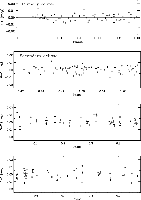
light curve are shown in Fig. 2.
As seen, the results from the four bands agree well.
Changing to Claret (2000)
limb darkening coefficients,
which are 0.07-0.09 higher, increases the radius of the primary
component
by only 0.4%, whereas that of the secondary component is increased
by 1.5%. This is linked to a 1% larger k and a 29%
smaller
residuals of the y observations from the
theoretical
light curve are shown in Fig. 2.
As seen, the results from the four bands agree well.
Changing to Claret (2000)
limb darkening coefficients,
which are 0.07-0.09 higher, increases the radius of the primary
component
by only 0.4%, whereas that of the secondary component is increased
by 1.5%. This is linked to a 1% larger k and a 29%
smaller ![]() ,
reducing e by 10%.
Limb darkening coefficients determined from the light curves reproduce
those by Van Hamme better than those by Claret, but have uncertainties
of about
,
reducing e by 10%.
Limb darkening coefficients determined from the light curves reproduce
those by Van Hamme better than those by Claret, but have uncertainties
of about ![]() 0.12.
Including non-linear limb darkening (logarithmic or
square-root law) has no significant effect on the photometric elements.
0.12.
Including non-linear limb darkening (logarithmic or
square-root law) has no significant effect on the photometric elements.
The adopted photometric elements listed in Table 7
are the weighted mean values of the JKTEBOP
solutions adopting the linear
limb darkening coefficients by Van Hamme. Realistic errors, based on
10 000 Monte Carlo simulations in each band and on comparison
between the uvby solutions, have been assigned.
The Monte Carlo simulations include random variations within ![]() 0.07
of the linear limb darkening coefficients.
As seen,
0.07
of the linear limb darkening coefficients.
As seen, ![]() becomes more accurate than
becomes more accurate than ![]() .
This is because it correlates
less with k, probably related to the secondary
eclipse being nearly total
for the adopted elements.
It should be noted that the ybv luminosity ratios
from the
light curve solutions agree very well with the spectroscopic light
ratio (Sect. 4).
.
This is because it correlates
less with k, probably related to the secondary
eclipse being nearly total
for the adopted elements.
It should be noted that the ybv luminosity ratios
from the
light curve solutions agree very well with the spectroscopic light
ratio (Sect. 4).
For comparison, Popper & Etzel (1981) obtained
![]() and
and
![]() ,
assuming
,
assuming ![]() and adopting
and adopting ![]() in order to
reproduce a mean ratio of
in order to
reproduce a mean ratio of ![]() between selected secondary and primary lines, measured on photographic
spectra. This ratio is, however, much higher than the light ratio we
derive from the FIES spectra, leading to a higher k.
Popper and Etzel also
obtain a somewhat larger value for
between selected secondary and primary lines, measured on photographic
spectra. This ratio is, however, much higher than the light ratio we
derive from the FIES spectra, leading to a higher k.
Popper and Etzel also
obtain a somewhat larger value for
![]() .
The relative radii presented by Demircan et al. (1994) are close to
those by Popper and Etzel.
.
The relative radii presented by Demircan et al. (1994) are close to
those by Popper and Etzel.
In conclusion, the new photometric elements derived from analyses of the uvby light curves are significantly more accurate than previous determinations. We find that the secondary eclipse is almost total, with 98% of the y light of the secondary component eclipsed, whereas about 57% of the y light from the primary component is eclipsed at phase 0.0.
6 Spectroscopic elements
Spectroscopic orbits have been derived from a re-analysis of the
radial velocities by Popper (1983)
and an analysis of the
new radial velocities listed in Table 4.
We have used the method of Lehman-Filhés implemented in the SBOP![]() program (Etzel 2004),
which is a modified and expanded version of
an earlier code by Wolfe et al. (1967).
The orbital period P was fixed at the ephemeris
value (Eq. (1)),
and the eccentricity e and longitude of periastron
program (Etzel 2004),
which is a modified and expanded version of
an earlier code by Wolfe et al. (1967).
The orbital period P was fixed at the ephemeris
value (Eq. (1)),
and the eccentricity e and longitude of periastron ![]() to
the results from the photometric analysis (Table 7). The
radial velocities of the components were analysed independently (SB1
solutions).
to
the results from the photometric analysis (Table 7). The
radial velocities of the components were analysed independently (SB1
solutions).
The spectroscopic elements are presented in Table 8.
The semiamplitudes (![]() ,
, ![]() ), and their
uncertainties, obtained from Popper's velocities are identical to his
results, even though he assumed the orbit to be circular and used an
older ephemeris.
), and their
uncertainties, obtained from Popper's velocities are identical to his
results, even though he assumed the orbit to be circular and used an
older ephemeris.
As seen, significantly more accurate semiamplitudes are
derived from the FIES velocities. They are slightly smaller than those
from Popper's velocities, but within errors the results agree.
Including e and/or ![]() as free parameters formally improves
the solution but does not alter the semiamplitudes. The number of
velocities is, however, too small for reliable spectroscopic
determination
of e and
as free parameters formally improves
the solution but does not alter the semiamplitudes. The number of
velocities is, however, too small for reliable spectroscopic
determination
of e and ![]() .
The double-lined (SB2) solutions agree perfectly with the single-lined
solutions listed in Table 8. Also,
spectroscopic elements determined as part of the spectral
disentangling (Sect. 7)
are identical.
We notice that the new system velocities (
.
The double-lined (SB2) solutions agree perfectly with the single-lined
solutions listed in Table 8. Also,
spectroscopic elements determined as part of the spectral
disentangling (Sect. 7)
are identical.
We notice that the new system velocities (
![]() ,
,
![]() )
differ by about 1 kms-1 from Popper's results.
This is probably due to radial velocity zero point differences.
Our velocities are tied to the ThAr exposures taken before and/or after
each target exposure. Standard star observations normally agree to
within 0.1-0.2 kms-1.
)
differ by about 1 kms-1 from Popper's results.
This is probably due to radial velocity zero point differences.
Our velocities are tied to the ThAr exposures taken before and/or after
each target exposure. Standard star observations normally agree to
within 0.1-0.2 kms-1.
Table 6: Photometric solutions for BK Peg from the JKTEBOP code.
Table 7: Adopted photometric elements for BK Peg.
|
Figure 2:
(
|
| Open with DEXTER | |
Table 8: Spectroscopic orbital solutions for BK Peg.
|
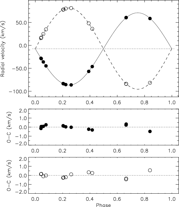
Figure 3: Spectroscopic orbital solution for BK Peg (solid line: primary; dashed line: secondary) and radial velocities (filled circles: primary; open circles: secondary). The dotted line ( upper panel) represents the center-of-mass velocity of the system. Phase 0.0 corresponds to central primary eclipse. |
| Open with DEXTER | |
7 Chemical abundances
For abundance analyses, we have disentangled the FIES spectra of BK Peg in order to extract the individual component spectra. We have applied the disentangling method introduced by Simon & Sturm (1994) and a revised version of the corresponding original code developed by E. Sturm. It assumes a constant light level, but since BK Peg is constant to within 0.5% outside of eclipses this is of no concern. Twenty-two orders, covering 5160-6450 Å (with a few gaps) were selected and disentangled individually. The orbital elements were fixed at the adopted values (Table 8) and very slightly wavelength dependent light ratios matching the results from the light curve analyses (Table 7) were adopted. Around 6070 Å, the signal-to-noise ratios of the resulting component spectra are 160 (primary) and 80 (secondary). A 40 Å region, centred at 6070 Å, is shown in Fig. 4.
The basic approach followed in the abundance analyses is described by CTB08. We used the versatile VWA tool, which applies the SYNTH software (Valenti & Piskunov 1996) to compute synthetic spectra. We refer to Bruntt et al. (2004,2008) and Bruntt (2009) for a detailed description of VWA. Atmosphere models were interpolated from the recent grid of MARCS model atmospheres (Gustafsson et al. 2008), which adopt the solar composition by Grevesse et al. (2007). Atomic line data are from the Vienna Atomic Line Database (VALD; Kupka et al. 1999), but in order to derive abundances relative to the Sun, log(gf) values have been adjusted in such a way that each measured line in the Wallace et al. (1998) Solar atlas reproduces the atmospheric abundances by Grevesse et al. (2007).
The abundance results derived from all useful lines with
equivalent
widths between 10 and 100 mÅ are presented in Table 9.
The equivalent widths measured in the disentangled spectra are listed
in Tables 14 (primary) and 15 (secondary), which will only be
available
in electronic form.
The surface gravities and observed rotational velocities listed in
Table 10
were adopted, whereas the effective temperatures
and microturbulence velocities were tuned until Fe I
abundances were
independent of line equivalent widths and excitation potentials.
The resulting temperatures are
![]() K
(primary) and
K
(primary) and
![]() K (secondary).
From a study of 10 F-K type stars with interferometrically and
spectroscopically determined effective temperatures, Bruntt
et al. (2010)
find a systematic offset of 40 K, which should be subtracted.
The corrected spectroscopic temperatures are still
slightly higher than derived from the uvby indices
(Table 10)
but agree within errors.
K (secondary).
From a study of 10 F-K type stars with interferometrically and
spectroscopically determined effective temperatures, Bruntt
et al. (2010)
find a systematic offset of 40 K, which should be subtracted.
The corrected spectroscopic temperatures are still
slightly higher than derived from the uvby indices
(Table 10)
but agree within errors.
Microturbulence velocities of
![]() kms-1
(primary) and
kms-1
(primary) and
![]() kms-1
(secondary) were obtained.
The calibration by Edvardsson et al. (1993) predicts higher
values of
kms-1
(secondary) were obtained.
The calibration by Edvardsson et al. (1993) predicts higher
values of
![]() kms-1
(primary) and
kms-1
(primary) and ![]() kms-1 (secondary);
the difference in microturbulence will be discussed by Bruntt
et al.
(2010).
kms-1 (secondary);
the difference in microturbulence will be discussed by Bruntt
et al.
(2010).
![\begin{figure}
\par\includegraphics[width=16cm,clip]{14266f04.ps}
\end{figure}](/articles/aa/full_html/2010/08/aa14266-10/img121.png)
|
Figure 4: A 40 Å region centred at 6070 Å of the disentangled spectra of the components of BK Peg. Lines identified by a red line were not used for the abundance analysis. |
| Open with DEXTER | |
Table 9:
Abundances (
![]() )
for the primary and secondary
components of BK Peg.
)
for the primary and secondary
components of BK Peg.
As seen, a robust ![]() is obtained, with nearly identical
results from Fe I and
Fe II lines of both
components.
The mean value from all measured Fe lines is
is obtained, with nearly identical
results from Fe I and
Fe II lines of both
components.
The mean value from all measured Fe lines is
![]()
![]() (rms of mean).
Changing the model temperatures by
(rms of mean).
Changing the model temperatures by ![]() K modifies
K modifies
![]() from the
Fe I lines by
about
from the
Fe I lines by
about ![]() dex, whereas almost no
effect is seen for Fe II
lines.
If 0.25 kms-1 higher microturbulence velocities
are adopted,
dex, whereas almost no
effect is seen for Fe II
lines.
If 0.25 kms-1 higher microturbulence velocities
are adopted,
![]() decreases by about 0.04 dex
for both neutral and ionized lines.
Taking these contributions to the uncertainties into account,
we adopt
decreases by about 0.04 dex
for both neutral and ionized lines.
Taking these contributions to the uncertainties into account,
we adopt ![]()
![]() for BK Peg.
In general, we find similar relative abundances for the other ions
listed in Table 9,
including the
for BK Peg.
In general, we find similar relative abundances for the other ions
listed in Table 9,
including the
![]() -elements
Si, Ca, and Ti.
-elements
Si, Ca, and Ti.
As an addition to the spectroscopic abundance analysis, we
have
also calculated metal abundances from the de-reddened uvby
indices for the
individual components (Table 10) and
the calibration by Holmberg et al. (2007).
The results are: ![]()
![]() (primary) and
(primary) and
![]()
![]() (secondary). Within errors
they agree with
those from the spectroscopic analysis;
the quoted
(secondary). Within errors
they agree with
those from the spectroscopic analysis;
the quoted ![]() errors include the uncertainties of the
photometric indices and the published spread of the calibration.
errors include the uncertainties of the
photometric indices and the published spread of the calibration.
Table 10: Astrophysical data for BK Peg.
8 Absolute dimensions
Absolute dimensions for BK Peg are presented in Table 10, as calculated from the photometric and spectroscopic elements given in Tables 7 and 8. As seen, masses and radii precise to 0.4-0.5% and 0.4-1.2%, respectively, have been established for the binary components.
The V magnitudes and uvby indices for the components, included in Table 10, were calculated from the combined magnitude and indices of the system outside eclipses (Table 1) and the luminosity ratios between the components (Table 7). Within errors, the V magnitude and the uvby indices of the primary component agree with those measured at central secondary eclipse where 98% (y) of the light from the secondary component eclipsed (cf. Table 1).
The interstellar reddening
![]() ,
also given in
Table 10,
was determined from the calibration by Olsen (1988), using the
,
also given in
Table 10,
was determined from the calibration by Olsen (1988), using the ![]() standard photometry for the combined light outside eclipses.
Within errors, the same reddening is obtained from the indices observed
during the central part of secondary eclipse.
The new intrinsic-colour calibration by Karatas & Schuster (2009)
leads to E(b-y)
= 0.034.
The model by Hakkila et al. (1997)
yields a higher reddening of
E(B-V)
= 0.14 or E(b-y)
= 0.10 in
the direction of and at the distance of BK Peg, whereas the
maps by
Burstein & Heiles (1982)
and Schlegel et al. (1998)
give
total E(B-V)
reddenings of 0.07 and 0.05, respectively.
standard photometry for the combined light outside eclipses.
Within errors, the same reddening is obtained from the indices observed
during the central part of secondary eclipse.
The new intrinsic-colour calibration by Karatas & Schuster (2009)
leads to E(b-y)
= 0.034.
The model by Hakkila et al. (1997)
yields a higher reddening of
E(B-V)
= 0.14 or E(b-y)
= 0.10 in
the direction of and at the distance of BK Peg, whereas the
maps by
Burstein & Heiles (1982)
and Schlegel et al. (1998)
give
total E(B-V)
reddenings of 0.07 and 0.05, respectively.
From the individual indices and the calibration by Holmberg
et al. (2007),
we derive effective temperatures of
![]() and
and
![]() K
for the primary
and secondary
component, respectively, assuming the final
K
for the primary
and secondary
component, respectively, assuming the final
![]() abundance.
The temperature uncertainties include those of the uvby
indices, E(b-y),
abundance.
The temperature uncertainties include those of the uvby
indices, E(b-y),
![]() ,
and the calibration itself.
Compared to this, the empirical flux scale by Popper (1980) and the y
flux ratio between the components (Table 7)
yield a well established temperature difference between the components
of
,
and the calibration itself.
Compared to this, the empirical flux scale by Popper (1980) and the y
flux ratio between the components (Table 7)
yield a well established temperature difference between the components
of
![]() K
(excluding possible errors of the scale itself).
Consequently, we assign temperatures of 6265 and 6320 K, which
agree with
the corrected spectroscopic results, 6325 and 6345 K, within
errors (Sect. 7).
As seen from Table 5
(combined light), temperatures from the (b-y),
c1 calibration by Alonso
et al. (1996)
and the b-y calibration by
Ramírez & Meléndez (2005)
are in perfect agreement with that from the Holmberg et al.
calibration.
K
(excluding possible errors of the scale itself).
Consequently, we assign temperatures of 6265 and 6320 K, which
agree with
the corrected spectroscopic results, 6325 and 6345 K, within
errors (Sect. 7).
As seen from Table 5
(combined light), temperatures from the (b-y),
c1 calibration by Alonso
et al. (1996)
and the b-y calibration by
Ramírez & Meléndez (2005)
are in perfect agreement with that from the Holmberg et al.
calibration.
The measured rotational velocity for the secondary component is in perfect agreement with (pseudo)synchronous rotation, whereas the primary component seems to rotate at a slightly lower rate.
The distance to BK Peg was calculated from the
``classical'' relation (see e.g. CTB08),
adopting the solar values and bolometric corrections given in
Table 10,
and AV/E(b-y)
= 4.28 (Crawford & Mandwewala 1976).
As seen, identical values are obtained for the two components, and the
distance has been established to 4%, accounting for all
error sources.
Nearly the same distance is obtained if other BC
scales, e.g.
Code et al. (1976),
Bessell et al. (1998)
and
Girardi et al. (2002),
are adopted.
Also, the empirical K surface brightness -
![]() relation
by Kervella et al. (2004)
leads to an identical and perhaps
even more precise (2%) distance. We refer to Clausen (2004) and Southworth
et al. (2005)
for details on the use of eclipsing binaries as standard candles.
relation
by Kervella et al. (2004)
leads to an identical and perhaps
even more precise (2%) distance. We refer to Clausen (2004) and Southworth
et al. (2005)
for details on the use of eclipsing binaries as standard candles.
9 Comparison with stellar models
Table 11: Model parameters and average ages for BK Peg inferred from the observed masses and radii.
In the following, we compare the absolute dimensions obtained
for BK Peg with properties of recent theoretical stellar
evolutionary models.
We have concentrated on the Yonsei-Yale (Y2)
grids by Demarque et al.
(2004)![]() and the VRSS (scaled-solar
abundances of the heavy elements) Victoria-Regina grids (VandenBerg
et al. 2006)
and the VRSS (scaled-solar
abundances of the heavy elements) Victoria-Regina grids (VandenBerg
et al. 2006)![]() listed in Table 11.
The abundance, mass, and age interpolation routines
provided by the Y2 group and
the isochrone interpolation routines provided by the Victoria-Regina
group have been applied.
A summary of the Y2 and VRSS
grids and their input physics is given by CTB08. Here we just recall
the following: The Y2 models
include He diffusion,
whereas diffusion processes are not included in the VRSS models.
The Y2 models adopt the
enrichment law Y
= 0.23 + 2Z together with the solar mixture by
Grevesse et al. (1996),
and the VRSS models Y
= 0.23544 + 2.2Z and the solar mixture by Grevesse
& Noels (1993).
listed in Table 11.
The abundance, mass, and age interpolation routines
provided by the Y2 group and
the isochrone interpolation routines provided by the Victoria-Regina
group have been applied.
A summary of the Y2 and VRSS
grids and their input physics is given by CTB08. Here we just recall
the following: The Y2 models
include He diffusion,
whereas diffusion processes are not included in the VRSS models.
The Y2 models adopt the
enrichment law Y
= 0.23 + 2Z together with the solar mixture by
Grevesse et al. (1996),
and the VRSS models Y
= 0.23544 + 2.2Z and the solar mixture by Grevesse
& Noels (1993).
|
Figure 5:
Comparison between Y2
(black) and VRSS (red) models for
|
| Open with DEXTER | |
|
Figure 6:
Comparison between Y2 (solid
lines, black) and VRSS (dashed lines, red) models for
|
| Open with DEXTER | |
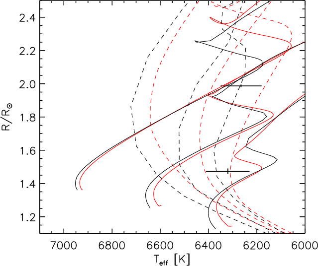
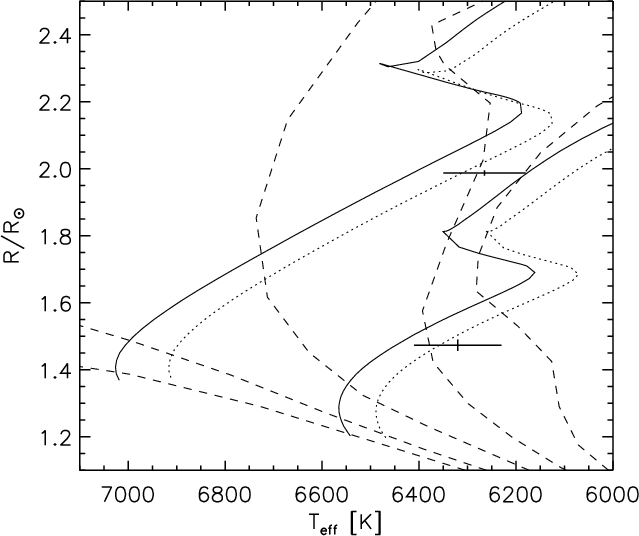
In Fig. 5, we
compare Y2 and VRSS
main-sequence evolutionary tracks and isochrones for
![]() =-0.105
=-0.105![]() in the mass region of BK Peg. For 1.3
in the mass region of BK Peg. For 1.3 ![]() the tracks nearly coincide, whereas the TAMS positions differ for both
lower and higher masses, probably related to the individual core
overshoot
recipes. In addition, somewhat different ages are predicted along the
main-sequence
tracks. This is also illustrated by the isochrones in the mass-radius
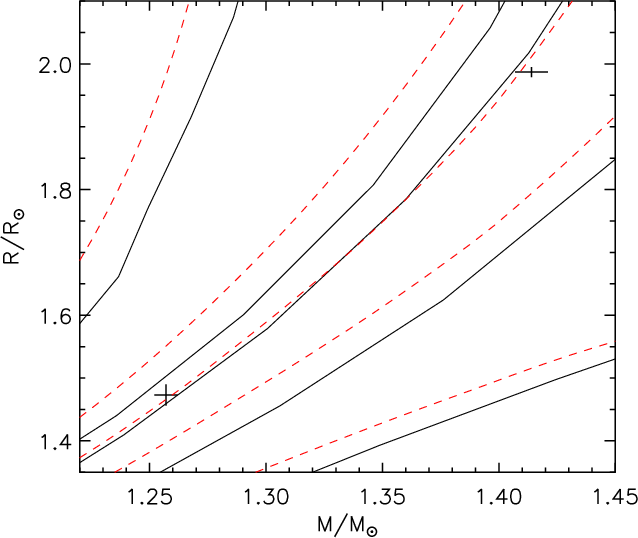
diagram shown in Fig. 6, which
represents the most direct
comparison with BK Peg, since the observed masses and radii
are scale independent.
As seen, similar ages of 2.75 (Y2)
and 2.50 (VRSS) Gyr are predicted for
the components, with a slight preference for the shape of the VRSS
isochrone. Within the observed metal abundance range,
the tracks nearly coincide, whereas the TAMS positions differ for both
lower and higher masses, probably related to the individual core
overshoot
recipes. In addition, somewhat different ages are predicted along the
main-sequence
tracks. This is also illustrated by the isochrones in the mass-radius
diagram shown in Fig. 6, which
represents the most direct
comparison with BK Peg, since the observed masses and radii
are scale independent.
As seen, similar ages of 2.75 (Y2)
and 2.50 (VRSS) Gyr are predicted for
the components, with a slight preference for the shape of the VRSS
isochrone. Within the observed metal abundance range,
![]()
![]() ,
the best fitting isochrones reproduce BK Peg nearly equally
well; the corresponding average ages are listed in Table 11.
,
the best fitting isochrones reproduce BK Peg nearly equally
well; the corresponding average ages are listed in Table 11.
|
Figure 7:
BK Peg compared with Y2
models for |
| Open with DEXTER | |
Y2 tracks for the observed masses and abundance of BK Peg are shown in Fig. 7. They are, like the VRSS tracks, slightly hotter. We also recall that the temperatures derived as part of the spectroscopic abundance analysis are slightly higher than those adopted from the uvbyindices (Table 10).
In conclusion, the Y2
and Victoria-Regina VRSS models, including
their core overshoot treatment and ramping recipes, are able to
reproduce
the observed properties of BK Peg. We note, however, that both
grids predict a slightly lower age for the 1.41 ![]() primary component than for the 1.26
primary component than for the 1.26 ![]() secondary.
In the following section, we will check whether this tendency is seen
for other
well-studied binaries with similar component masses.
secondary.
In the following section, we will check whether this tendency is seen
for other
well-studied binaries with similar component masses.
10 Comparison with other binaries
The review on accurate masses and radii of normal stars by Torres et al. (2010) lists 20 binariesTable 12:
Masses, radii, and abundances from Torres et al. (2010) for a subset of
well-studied binaries with both components in the 1.15-1.70 ![]() interval; see the text for details.
interval; see the text for details.
|
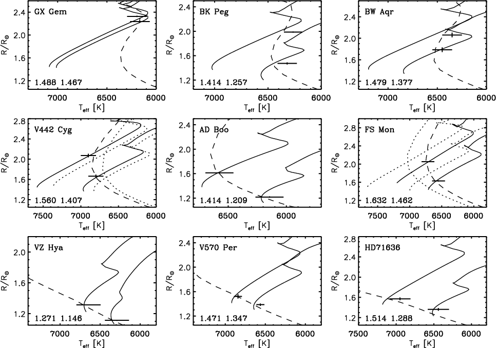
Figure 8:
Y2 evolutionary tracks
(full drawn lines) for the binaries included in Table 12. The
isochrones (dashed lines) correspond to the
average ages inferred from the masses and radii for the
|
| Open with DEXTER | |
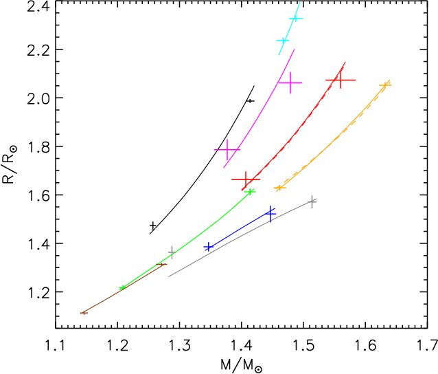
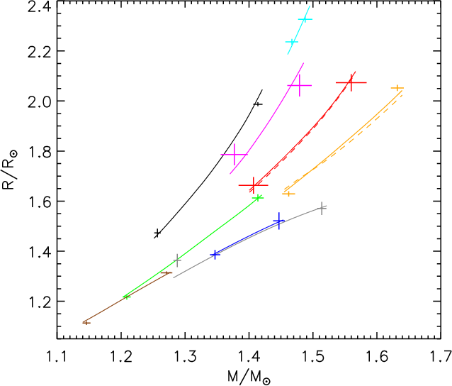
In Figs. 9
(Y2) and 10
(VRSS), we concentrate on comparisons based on the scale-independent
masses and radii. Since abundance interpolation
software is not available for the VRSS models, we have used those with
![]() closest to
the measured values.
The average ages are listed in Table 12, and we note
the following:
closest to
the measured values.
The average ages are listed in Table 12, and we note
the following:
- The VRSS models predict lower ages than the Y2 models for all systems.
- For the four binaries with components in the upper half of
the main-sequence band
(GX Gem, BK Peg, BW Aqr, V442 Cyg),
both grids tend to predict lower ages for the more massive component
than for the less massive one, although the difference is
certainly very marginal for the nearly equal-mass system
GX Gem. These systems span the 1.26-1.56
 interval.
- The Y2
isochrones fit FS Mon (1.63 + 1.46 )
better than the VRSS isochrones,
which predict a higher age for the more massive component than for the
less
massive one.
- Both grids fit the less evolved binaries BW Aqr and BW Aqr quite well, perhaps with a slight preference for Y2.
- For the little evolved binary BW Aqr, VRSS is marginally better than Y2.
- HD 71636 is not fitted well by any of the grids.
The very different ages predicted for the components are listed in
Table 12.
We believe,
however, that this is due to problems with the published radii. A
re-analysis
of the light curves by Henry et al. (2006) indicates that
the ratio
between the (relative) radii is significantly more uncertain than given
by the
authors,
most probably because the secondary eclipse is far from being
well-covered.
It is outside the scope of this paper to propose specific modifications of the model physics, but we believe that this sample of binaries (except HD 71636) can be used to fine-tune the core overshoot treatment in terms of mass and metal abundance. It might also be relevant to include investigations of other model ingredients, e.g. diffusion processes and the adopted helium-to-metal enrichment ratio, and to clarify why the Y2 models predict higher ages than the VRSS models. In order to avoid possible interpolation errors, specific models for the observed masses and metal abundances should be calculated and small age steps applied. On the observational side, spectroscopic metal abundances should be determined for the four binaries lacking this information, and it should perhaps be considered to re-observe BW Aqr, V442 Cyg, and HD 71636 to improve their masses and/or radii.
|
Figure 9:
Comparison between Y2
isochrones (full drawn lines) and the binaries listed in Table 12; we refer to
the table for colour codes, |
| Open with DEXTER | |
|
Figure 10:
Comparison between VRSS isochrones (full drawn lines) and the binaries
listed in Table 12;
we refer to the table for colour codes,
|
| Open with DEXTER | |
Also, we suggest to supplement the sample by the unique K0IV+F7V binary
AI Phe (1.23+1.19 ![]() ), recently re-discussed by
Torres et al. (2010),
as well as by a number of new F-type systems we are presently studying.
In addition, it would be highly relevant to include F-type binary
members of open clusters.
), recently re-discussed by
Torres et al. (2010),
as well as by a number of new F-type systems we are presently studying.
In addition, it would be highly relevant to include F-type binary
members of open clusters.
11 Summary and conclusions
From state-of-the-art observations and analyses, precise (0.4-1.2%)
absolute
dimensions have been established for the components of the late F-type
detached eclipsing binary BK Peg (
![]() ,
e = 0.0053);
see Table 10.
A detailed spectroscopic analysis yields an iron abundance relative to
the Sun
of
,
e = 0.0053);
see Table 10.
A detailed spectroscopic analysis yields an iron abundance relative to
the Sun
of ![]()
![]() and similar relative
abundances for Si, Ca, Sc, Ti, Cr,
and Ni.
The measured rotational velocities are
and similar relative
abundances for Si, Ca, Sc, Ti, Cr,
and Ni.
The measured rotational velocities are
![]() (primary)
and
(primary)
and
![]() (secondary) kms-1.
For the secondary component
this corresponds
to (pseudo)synchronous rotation, whereas the primary component seems to
rotate at a slightly lower rate.
(secondary) kms-1.
For the secondary component
this corresponds
to (pseudo)synchronous rotation, whereas the primary component seems to
rotate at a slightly lower rate.
The 1.41 and 1.26 ![]() components of BK Peg have evolved to the upper half of the
main-sequence band. Yonsei-Yale and Victoria-Regina solar scaled
evolutionary models for the
observed metal abundance reproduce BK Peg at ages of 2.75 and
2.50 Gyr, respectively, but tend to predict a lower age for
the more massive primary component than for the secondary.
If real, this might be due to less than perfect calibration of the
amount of
convective core overshoot of the models as function of mass (and metal
abundance).
components of BK Peg have evolved to the upper half of the
main-sequence band. Yonsei-Yale and Victoria-Regina solar scaled
evolutionary models for the
observed metal abundance reproduce BK Peg at ages of 2.75 and
2.50 Gyr, respectively, but tend to predict a lower age for
the more massive primary component than for the secondary.
If real, this might be due to less than perfect calibration of the
amount of
convective core overshoot of the models as function of mass (and metal
abundance).
For this reason, we have performed model comparisons for a
sample of eight additional well-studied binaries with component masses
in the 1.15-1.70 ![]() interval where convective core overshoot is gradually ramped up in
the models; see Table 12.
We find that a) the Yonsei-Yale models systematically predict higher
ages than the Victoria-Regina models, and that b) the three other most
evolved systems in the sample share the age difference trend seen for
BK Peg.
interval where convective core overshoot is gradually ramped up in
the models; see Table 12.
We find that a) the Yonsei-Yale models systematically predict higher
ages than the Victoria-Regina models, and that b) the three other most
evolved systems in the sample share the age difference trend seen for
BK Peg.
We propose to use the sample to fine-tune the core overshoot
treatment, as well as other model ingredients, and to clarify why the
two model grids predict different ages. The sample should be expanded
by a number of new F-type systems under study, binary cluster members,
and the unique K0IV+F7V binary AI Phe (1.23+1.19 ![]() ).
).
It is a great pleasure to thank the many colleagues and students, who have shown interest in our project and have participated in the extensive (semi)automatic observations of BK Peg at the SAT: Sylvain Bouley, Christian Coutures, Thomas H. Dall, Mathias P. Egholm, Pascal Fouque, Lisbeth F. Grove, Anders Johansen, Erling Johnsen, Bjarne R. Jørgensen, Bo Milvang-Jensen, Alain Maury, John D. Pritchard, and Samuel Regandell. Excellent technical support was received from the staffs of Copenhagen University and ESO, La Silla. We thank J. M. Kreiner for providing a complete list of published times of eclipse for BK Peg. A. Kaufer, O. Stahl, S. Tubbesing, and B. Wolf kindly obtained the two FEROS spectra of BW Aqr during Heidelberg/Copenhagen guaranteed time in 1999.
The projects ``Stellar structure and evolution - new challenges from ground and space observations'' and ``Stars: Central engines of the evolution of the Universe'', carried out at Copenhagen University and Aarhus University, are supported by the Danish National Science Research Council.
The following internet-based resources were used in research for this paper: the NASA Astrophysics Data System; the SIMBAD database and the VizieR service operated by CDS, Strasbourg, France; the ariv scientific paper preprint service operated by Cornell University; the VALD database made available through the Institute of Astronomy, Vienna, Austria; the MARCS stellar model atmosphere library. This publication makes use of data products from the Two Micron All Sky Survey, which is a joint project of the University of Massachusetts and the Infrared Processing and Analysis Center/California Institute of Technology, funded by the National Aeronautics and Space Administration and the National Science Foundation.
Appendix A: Chemical abundances for BW Aqr
Absolute dimensions for the late F-type eclipsing binary BW Aqr were published by Clausen (1991), who mentioned that theHere we present the results from an abundance
analysis based on two high-resolution spectra observed with the FEROS
fibre echelle spectrograph at ESO, La Silla in August 1999; see
Table A.1.
Details on the spectrograph, the reduction of the spectra,
and the basic approach followed in the abundance analysis are
described by CTB08.
As for BK Peg, we have used the VWA tool for the abundance
analysis,
and we refer to Sect. 7
for further information on atmosphere
models, atomic data information, ![]() )
adjustments etc. One important difference is, however, that for
BW Aqr disentangling is not possible, and the analysis is
therefore based on double-lined spectra.
)
adjustments etc. One important difference is, however, that for
BW Aqr disentangling is not possible, and the analysis is
therefore based on double-lined spectra.
The effective temperatures, surface gravities, rotational
velocities, and
microturbulence velocities listed in Table A.2 were
adopted.
The temperatures were determined by requiring that Fe I
abundances were
independent of line excitation potentials. They are slightly lower than
determined by Clausen (1991),
who obtained ![]() K (primary)
and
K (primary)
and ![]() K (secondary). However, new and better (unpublished) uvby
photometry for BW Aqr and the calibration by Holmberg
et al. (2007)
lead
to 100 K lower values, assuming a reddening of
E(b-y)
= 0.03.
Microturbulence velocities were tuned until Fe I
abundances are
independent of line equivalent widths.
K (secondary). However, new and better (unpublished) uvby
photometry for BW Aqr and the calibration by Holmberg
et al. (2007)
lead
to 100 K lower values, assuming a reddening of
E(b-y)
= 0.03.
Microturbulence velocities were tuned until Fe I
abundances are
independent of line equivalent widths.
The abundances derived from all useful lines in both spectra
are presented in Table A.3.
The equivalent widths measured in the two double-lined spectra are
listed
in Tables 16 (primary) and 17 (secondary), which will only be
available in
electronic form.
Comparing the results from the two spectra, we find that they agree
within
0.05 dex. We have only included lines with measured
equivalent
widths above 10 mÅ and below 45 mÅ (primary) and 55 mÅ (secondary).
The lines are diluted by factors of about 2.2 (primary)
and 1.8 (secondary), meaning that lines with intrinsic
strengths
above 100 mÅ are excluded.
The ![]() results for the two components differ by 0.06 dex, but for each
component the results from Fe I
and Fe II lines agree
well. The mean value for all measured Fe lines is
results for the two components differ by 0.06 dex, but for each
component the results from Fe I
and Fe II lines agree
well. The mean value for all measured Fe lines is
![]() =
=
![]() (rms of mean).
(rms of mean).
Table A.1: Log of the FEROS observations of BW Aqr.
Table A.2: Astrophysical data adopted for the abundance analysis of BW Aqr.
Table A.3:
Abundances (
![]() )
for the primary and secondary
components of BW Aqr determined from the two FEROS spectra.
)
for the primary and secondary
components of BW Aqr determined from the two FEROS spectra.
Changing the model temperatures by ![]() K modifies
K modifies
![]() from the
Fe I lines by
about
from the
Fe I lines by
about ![]() dex, whereas almost no
effect is seen for the Fe II
lines.
If 0.30 kms-1 higher microturbulence velocities
are adopted,
dex, whereas almost no
effect is seen for the Fe II
lines.
If 0.30 kms-1 higher microturbulence velocities
are adopted,
![]() decreases by about 0.05 dex
for both neutral and ionized lines.
Taking these contributions to the uncertainties into account,
we adopt
decreases by about 0.05 dex
for both neutral and ionized lines.
Taking these contributions to the uncertainties into account,
we adopt ![]()
![]() for BW Aqr.
Similar abundances are obtained for the few other ions listed in
Table A.3.
for BW Aqr.
Similar abundances are obtained for the few other ions listed in
Table A.3.
References
- Ak, H., Ozerer, F. F., & Ekmekci, F. 2003, Inf. Bull. Var. Stars, 5361 [Google Scholar]
- Alonso, A., Arribas, S., & Martínez-Roger, C. 1996, A&A, 313, 873 [NASA ADS] [Google Scholar]
- Andersen, J., Nordström, B., & Clausen, J. V. 1990, ApJ, 363, L33 [NASA ADS] [CrossRef] [Google Scholar]
- Bessell, M. S., Castelli, F., & Plez, B. 1998, A&A, 333, 231 [NASA ADS] [Google Scholar]
- Braune, W., & Hübscher, J. 1987, BAV Mitteilungen, 46 [Google Scholar]
- Bruntt, H. 2009, A&A, 506, 235 [NASA ADS] [CrossRef] [EDP Sciences] [Google Scholar]
- Bruntt, H., Bikmaev, I. F., Catala, C., et al. 2004, A&A, 425, 683 [NASA ADS] [CrossRef] [EDP Sciences] [Google Scholar]
- Bruntt, H., De Cat, P., & Aerts, C. 2008, A&A, 478, 487 [NASA ADS] [CrossRef] [EDP Sciences] [Google Scholar]
- Bruntt, H., Bedding, T. R., Quirion, P.-O., et al. 2010, MNRAS, accepted [arXiv:10024268] [Google Scholar]
- Burstein, D., & Heiles, C. 1982, AJ, 87, 1165 [NASA ADS] [CrossRef] [Google Scholar]
- Claret, A. 2000, A&A, 363, 1081 [NASA ADS] [Google Scholar]
- Claret, A. 2007, A&A, 475, 1019 [NASA ADS] [CrossRef] [EDP Sciences] [Google Scholar]
- Clausen, J. V. 1991, A&A, 246, 397 [NASA ADS] [Google Scholar]
- Clausen, J. V. 2004, New A. Rev., 48, 679 [Google Scholar]
- Clausen, J. V., Helt, B. E., & Olsen, E. H. 2001, A&A, 374, 980 (CHO01) [NASA ADS] [CrossRef] [EDP Sciences] [Google Scholar]
- Clausen, J. V., Torres, G., Bruntt, H., et al. 2008b, A&A, 487, 1095 (CTB08) [NASA ADS] [CrossRef] [EDP Sciences] [Google Scholar]
- Clausen, J. V., Olsen, E. H., Helt, B. E., & Claret, A. 2010, A&A, 510, A91 [NASA ADS] [CrossRef] [EDP Sciences] [Google Scholar]
- Code, A. D., Bless, R. C., Davis, J., & Brown, R. H. 1976, ApJ, 203, 417 [NASA ADS] [CrossRef] [Google Scholar]
- Crawford, D. L., & Mandwewala, N. 1976, PASP, 88, 917 [NASA ADS] [CrossRef] [Google Scholar]
- Demarque, P., Woo, J.-H., Kim, Y.-C., & Yi, S. K. 2004, ApJS, 155, 667 [NASA ADS] [CrossRef] [Google Scholar]
- Demircan, O., Kaya, Y., & Tüfekcioglu, Z. 1994, Ap&SS, 222, 213 [NASA ADS] [CrossRef] [Google Scholar]
- Diethelm, R. 2001, in BBSAG Bulletin, 126 [Google Scholar]
- Dworak, T. Z. 1977, Acta Astron., 27, 151 [NASA ADS] [Google Scholar]
- Edvardsson, B., Andersen, J., Gustafsson, B., et al. 1993, A&A, 275, 101 [NASA ADS] [Google Scholar]
- Etzel P. B. 1981, in Photometric and Spectroscopic Binary Systems, ed. E. B. Carling, & Z. Kopal, (NATO), 111 [Google Scholar]
- Etzel, P. B. 2004, SBOP: Spectroscopic Binary Orbit Program (San Diego State University) [Google Scholar]
- Flower, P. J. 1996, ApJ, 469, 355 [NASA ADS] [CrossRef] [Google Scholar]
- Girardi, L., Bertelli, G., Bressan, A., et al. 2002, A&A, 391, 195 [NASA ADS] [CrossRef] [EDP Sciences] [Google Scholar]
- Grevesse, N., & Noels, A. 1993, Phys. Scr. T47, 133 [Google Scholar]
- Grevesse, N., & Sauval, A. J. 1998, Space Sci. Rev., 85, 161 [NASA ADS] [CrossRef] [Google Scholar]
- Grevesse, N., Noels, A., & Sauval, A. J. 1996, in Cosmic Abundances, ed. S. S. Holt, & G. Sonneborn (San Francisco: ASP), 117 [Google Scholar]
- Grevesse, N., Asplund, M., & Sauval, A. J. 2007, Space Sci. Rev., 130, 105 [Google Scholar]
- Griffin, R. F. 2007, The Observatory, 127, 113 [NASA ADS] [Google Scholar]
- Gustafsson, B., Edvardsson, B., Eriksson, K., et al. 2008, A&A, 486, 951 [NASA ADS] [CrossRef] [EDP Sciences] [Google Scholar]
- Hakkila, J., Myers, J. M., Stidham, B. J., & Hartmann, D. H. 1997, AJ, 114, 2043 [NASA ADS] [CrossRef] [Google Scholar]
- Harlan, E. A. 1969, AJ, 74, 916 [NASA ADS] [CrossRef] [Google Scholar]
- Harlan, E. A., & Taylor, D. C. 1970, AJ, 75, 507 [NASA ADS] [CrossRef] [Google Scholar]
- Heard, J. F. 1956, Publ. David Dunlop Obs., 2, 105 [Google Scholar]
- Heiter, U., Kupka, F., van't Menneret, C., et al. 2002, A&A, 392, 619 [NASA ADS] [CrossRef] [EDP Sciences] [Google Scholar]
- Henry, G. W., Fekel, F. C., Sowell, J. R., & Gearhart, J. S. 2006, AJ, 132, 2489 [NASA ADS] [CrossRef] [Google Scholar]
- Hoffmeister, C. 1931, AN 242, 129 [Google Scholar]
- Holmberg, J., Nordström, B., & Andersen, J. 2007 A&A, 475, 519 [Google Scholar]
- Hübscher, J., & Walter, F. 2007, Inf. Bull. Var. Stars, 5761 [Google Scholar]
- Jordi, C., Figueras, F., Torra, J., & Asiain, R. 1996, A&AS, 115, 401 [NASA ADS] [Google Scholar]
- Kaluzny, J., Pych, W., Rucinski, S. M., & Thompson, I. B. 2006, , 56, 237 [Google Scholar]
- Karatas, Y., & Schuster, W. J. 2010, New Astron., 15, 444 [NASA ADS] [CrossRef] [Google Scholar]
- Kervella, P., Thévenin, F., Di Folco, E., & Ségransan, D. 2004, A&A, 426, 297 [NASA ADS] [CrossRef] [EDP Sciences] [Google Scholar]
- Kreiner, J. M. 2004, , 54, 207 [Google Scholar]
- Kreiner, J. M., Kim, C. H., & Nha, I. S. 2001, An Atlas of O-C Diagrams of Eclipsing Binary Stars (Krakow: Wydawnictwo Naukowe Akad. Pedagogicznej) [Google Scholar]
- Kupka, F., Piskunov, N., Ryabchikova, T. A., Stempels, H. C., & Weiss, W. 1999, A&AS, 138, 119 [NASA ADS] [CrossRef] [EDP Sciences] [MathSciNet] [PubMed] [Google Scholar]
- Lacy, C. H. S., Torres, G., & Claret, A. 2008, AJ, 135, 1757 [NASA ADS] [CrossRef] [Google Scholar]
- Lause, F. 1935, AN 257, 73 [Google Scholar]
- Lause, F. 1937, AN 263, 115 [Google Scholar]
- Martynov D. Ya. 1973, in Eclipsing Variable Stars, ed. V. P. Tsesevich, Israel Program for Scientific Translation, Jerusalem [Google Scholar]
- Masana, E., Jordi, C., & Ribas, I. 2006, A&A, 450, 735 [NASA ADS] [CrossRef] [EDP Sciences] [Google Scholar]
- Nelson B., & Davis W. 1972, ApJ, 174, 617 [NASA ADS] [CrossRef] [Google Scholar]
- Olsen, E. H. 1983, A&AS, 54, 55 [Google Scholar]
- Olsen, E. H. 1988, A&A, 189, 173 [NASA ADS] [Google Scholar]
- Olsen, E. H. 1994, A&AS, 106, 257 [Google Scholar]
- Perry, C. L. 1969, AJ, 74, 705 [NASA ADS] [CrossRef] [Google Scholar]
- Popper, D. M. 1980, ARA&A 18, 115 [NASA ADS] [CrossRef] [Google Scholar]
- Popper, D. M. 1983, AJ, 88, 124 [NASA ADS] [CrossRef] [Google Scholar]
- Popper, D. M., & Dumont, P. J. 1977, AJ, 82, 216 [NASA ADS] [CrossRef] [Google Scholar]
- Popper, D. M., & Etzel, P. B. 1981, AJ, 86, 102 [NASA ADS] [CrossRef] [Google Scholar]
- Popper, D. M., & Etzel, P. B. 1995, Ap&SS, 232, 139 [NASA ADS] [CrossRef] [Google Scholar]
- Ramírez, I., & Meléndez, J. 2005, AJ, 626, 465 [Google Scholar]
- Ribas, I., Jordi, C., & Giménez, A. 2000, MNRAS, 318, 55 [Google Scholar]
- Rucinski, S. M. 1999, in Precise Stellar Radial Velocities, ed. J. B. Hearnshaw, & C. D. Scarfe, IAU Coll. 170, ASP Conf. Ser., 185, 82 [Google Scholar]
- Rucinski, S. M. 2002, AJ, 124, 1746 [NASA ADS] [CrossRef] [Google Scholar]
- Rucinski, S. M. 2004, in Stellar Rotation, ed. A. Maeder, & P. Eenens, IAU Symp. 215, (San Francisco: ASP), 17 [Google Scholar]
- Schlegel, D. J., Finkbeiner, D. P., & Davis, M. 1998, ApJ, 500, 525 [NASA ADS] [CrossRef] [Google Scholar]
- Simon, K. P., & Sturm, E. 1994, A&A, 1994, 281 [Google Scholar]
- Southworth, J., Maxted, P. F. L., & Smalley, B. 2004a, MNRAS, 351, 1277 [NASA ADS] [CrossRef] [Google Scholar]
- Southworth, J., Zucker, S., Maxted, P. F. L., & Smalley, B. 2004b, MNRAS, 355, 986 [NASA ADS] [CrossRef] [Google Scholar]
- Southworth, J., Maxted, P. F. L., & Smalley, B. 2005, A&A, 429, 645 [NASA ADS] [CrossRef] [EDP Sciences] [Google Scholar]
- Torres, G., Andersen, J., & Giménez, A. 2010, A&A Rev., 18, 67 [NASA ADS] [CrossRef] [EDP Sciences] [Google Scholar]
- Valenti, J., & Piskunov, N. 1996, A&AS, 118, 595 [NASA ADS] [CrossRef] [EDP Sciences] [Google Scholar]
- VandenBerg, D. A., Bergbusch, P. A., & Dowler, P. D. 2006, ApJS, 162, 375 [NASA ADS] [CrossRef] [MathSciNet] [Google Scholar]
- Van Hamme, W. 1993, AJ, 106, 2096 [NASA ADS] [CrossRef] [Google Scholar]
- Wallace, L., Hinkle, K., & Livingston, W. 1998, An atlas of the spectrum of the solar photosphere from 13 500 to 28 000 cm-1 (3570 to 7405 A), Tucson, AZ: NOAO [Google Scholar]
- Wolfe, R. H., Horak, H. G., & Storer, N. W. 1967, in Modern Astrophysics: A Memorial to Otto Struve, ed. M. Hack, 251 [Google Scholar]
Footnotes
- ... overshoot
- Based on observations carried out at the Strömgren Automatic Telescope (SAT) and the 1.5m telescope (63.H-0080) at ESO, La Silla, and the Nordic Optical Telescope at La Palma
- ...
- Tables 13-17 are available in electronic form at the CDS via anonymous ftp to cdsarc.u-strasbg.fr (130.79.128.5) or via http://cdsweb.u-strasbg.fr/cgi-bin/qcat?J/A+A/516/A42
- ...2004)
- http://www.as.ap.krakow.pl/ephem
- ... package
- see http://www.not.iac.es for details on FIES and FIEStool.
- ... IDL
- http://www.ittvis.com/idl/index.asp
- ... JKTEBOP
- http://www.astro.keele.ac.uk/ jkt/
- ... SBOP
- Spectroscopic Binary Orbit Program, http://mintaka.sdsu.edu/faculty/etzel/
- ...2004)
- http://www.astro.yale.edu/demarque/yystar.html
- ...2006)
- http://www1.cadc-ccda.hia-iha.nrc-cnrc.gc.ca/cvo/ community/VictoriaReginaModels/
- ...

- Defined as ``the mass above which stars continue to have a substantial convective core even after the end of the pre-MS phase''.
- ...
![$[{\rm Fe/H}]$](/articles/aa/full_html/2010/08/aa14266-10/img3.png) =-0.105
=-0.105
- VRSS models
for the observed =-0.12
are not available
- ... binaries
- The 20 binaries can now be supplemented by BK Peg and V1130 Tau (Clausen et al. 2010).
- ...
authors
- We have used the larger errors listed by Torres et al. (2010), which also seem to be underestimated.
All Tables
Table 1: Photometric data for BK Peg and the comparison stars.
Table 2: Times of primary (P) and secondary (S) minima for BK Peg.
Table 3: Log of the FIES observations of BK Peg.
Table 4: Radial velocities of BK Peg and residuals from the final spectroscopic orbit presented in Table 8.
Table 5: Effective temperatures (K) for the combined light of BK Peg.
Table 6: Photometric solutions for BK Peg from the JKTEBOP code.
Table 7: Adopted photometric elements for BK Peg.
Table 8: Spectroscopic orbital solutions for BK Peg.
Table 9:
Abundances (
![]() )
for the primary and secondary
components of BK Peg.
)
for the primary and secondary
components of BK Peg.
Table 10: Astrophysical data for BK Peg.
Table 11: Model parameters and average ages for BK Peg inferred from the observed masses and radii.
Table 12:
Masses, radii, and abundances from Torres et al. (2010) for a subset of
well-studied binaries with both components in the 1.15-1.70 ![]() interval; see the text for details.
interval; see the text for details.
Table A.1: Log of the FEROS observations of BW Aqr.
Table A.2: Astrophysical data adopted for the abundance analysis of BW Aqr.
Table A.3:
Abundances (
![]() )
for the primary and secondary
components of BW Aqr determined from the two FEROS spectra.
)
for the primary and secondary
components of BW Aqr determined from the two FEROS spectra.
All Figures
|
|
Figure 1: y light curve and b-y and u-b colour curves (instrumental system) for BK Peg. |
| Open with DEXTER | |
| In the text | |
|
|
Figure 2:
(
|
| Open with DEXTER | |
| In the text | |
|
|
Figure 3: Spectroscopic orbital solution for BK Peg (solid line: primary; dashed line: secondary) and radial velocities (filled circles: primary; open circles: secondary). The dotted line ( upper panel) represents the center-of-mass velocity of the system. Phase 0.0 corresponds to central primary eclipse. |
| Open with DEXTER | |
| In the text | |
|
|
Figure 4: A 40 Å region centred at 6070 Å of the disentangled spectra of the components of BK Peg. Lines identified by a red line were not used for the abundance analysis. |
| Open with DEXTER | |
| In the text | |
|
|
Figure 5:
Comparison between Y2
(black) and VRSS (red) models for
|
| Open with DEXTER | |
| In the text | |
|
|
Figure 6:
Comparison between Y2 (solid
lines, black) and VRSS (dashed lines, red) models for
|
| Open with DEXTER | |
| In the text | |
|
|
Figure 7:
BK Peg compared with Y2
models for |
| Open with DEXTER | |
| In the text | |
|
|
Figure 8:
Y2 evolutionary tracks
(full drawn lines) for the binaries included in Table 12. The
isochrones (dashed lines) correspond to the
average ages inferred from the masses and radii for the
|
| Open with DEXTER | |
| In the text | |
|
|
Figure 9:
Comparison between Y2
isochrones (full drawn lines) and the binaries listed in Table 12; we refer to
the table for colour codes, |
| Open with DEXTER | |
| In the text | |
|
|
Figure 10:
Comparison between VRSS isochrones (full drawn lines) and the binaries
listed in Table 12;
we refer to the table for colour codes,
|
| Open with DEXTER | |
| In the text | |
Copyright ESO 2010
Current usage metrics show cumulative count of Article Views (full-text article views including HTML views, PDF and ePub downloads, according to the available data) and Abstracts Views on Vision4Press platform.
Data correspond to usage on the plateform after 2015. The current usage metrics is available 48-96 hours after online publication and is updated daily on week days.
Initial download of the metrics may take a while.