| Issue |
A&A
Volume 516, June-July 2010
|
|
|---|---|---|
| Article Number | A19 | |
| Number of page(s) | 11 | |
| Section | Interstellar and circumstellar matter | |
| DOI | https://doi.org/10.1051/0004-6361/200913743 | |
| Published online | 18 June 2010 | |
CO observations of symbiotic stellar systems![[*]](/icons/foot_motif.png)
V. Bujarrabal1 - J. Miko![]() ajewska2 - J. Alcolea3 - G. Quintana-Lacaci4
ajewska2 - J. Alcolea3 - G. Quintana-Lacaci4
1 - Observatorio Astronómico Nacional. Ap 112, 28803 Alcalá de Henares, Spain
2 -
N. Copernicus Astronomical Center, Bartycka 18, 00716 Warsaw, Poland
3 -
Observatorio Astronómico Nacional (IGN), Alfonso XII N![]() 3, 28014 Madrid, Spain
3, 28014 Madrid, Spain
4 -
Instituto de Radioastronomía Milimétrica (IRAM), Avda. Divina Pastora 7, 18012 Granada, Spain
Received 26 November 2009 / Accepted 23 February 2010
Abstract
Aims. We have studied the molecular content of the
circumstellar environs of symbiotic stellar systems, in particular of
the well know objects R Aqr and CH Cyg. The study of molecules in these
stars will help for understanding the properties of the very inner
shells around the cool stellar component from which molecular emission
is expected to come.
Methods. We performed mm-wave observations with the IRAM 30 m telescope of the 12CO J=1-0 and J=2-1, 13CO J=1-0 and J=2-1, and SiO J=5-4
transitions in the symbiotic stars R Aqr, CH Cyg, and HM Sge. The data
were analyzed by means of a simple analytical description of the
general properties of molecular emission from the inner shells around
the cool star. Numerical calculations of the expected line profiles
were also performed that took the level population and radiative
transfer under such conditions into account.
Results. Weak emission of 12CO J=1-0 and J=2-1 was detected in R Aqr and CH Cyg and a good line profile of 12CO J=2-1
in R Aqr was obtained. The intensities and profile shapes of the
detected lines are compatible with emission coming from a very small
shell around the Mira-type star, with a radius comparable to or
slightly smaller than the distance to the hot dwarf companion,
![]() cm.
We argue that other possible explanations are improbable. This region
probably shows properties similar to those characteristic of the inner
shells around standard AGB stars: outwards expansion at about
5-25 km s-1, with a significant acceleration of
the gas, temperatures decreasing with radius between about 1000 and 500
K, and densities
cm.
We argue that other possible explanations are improbable. This region
probably shows properties similar to those characteristic of the inner
shells around standard AGB stars: outwards expansion at about
5-25 km s-1, with a significant acceleration of
the gas, temperatures decreasing with radius between about 1000 and 500
K, and densities
![]() cm-3. Our model calculations are able to explain the asymmetric line shape observed in 12CO J=2-1
from R Aqr, in which the relatively weaker blue part of the profile
would result from selfabsorption by the outer layers (in the presence
of a velocity increase and a temperature decrease with radius). The
mass-loss rates are somewhat higher than in standard AGB stars, as
often happens for symbiotic systems. In R Aqr, we find that the total
mass of the CO emitting region is
cm-3. Our model calculations are able to explain the asymmetric line shape observed in 12CO J=2-1
from R Aqr, in which the relatively weaker blue part of the profile
would result from selfabsorption by the outer layers (in the presence
of a velocity increase and a temperature decrease with radius). The
mass-loss rates are somewhat higher than in standard AGB stars, as
often happens for symbiotic systems. In R Aqr, we find that the total
mass of the CO emitting region is
![]()
![]() ,
corresponding to
,
corresponding to ![]()
![]()
![]()
![]() yr-1
and compatible with results obtained from dust emission. Considering
other existing data on molecular emission, we suggest that the limited
extent of the molecule-rich gas in symbiotic systems is mainly due to
molecule photodissociation by the radiation of the hot dwarf star.
yr-1
and compatible with results obtained from dust emission. Considering
other existing data on molecular emission, we suggest that the limited
extent of the molecule-rich gas in symbiotic systems is mainly due to
molecule photodissociation by the radiation of the hot dwarf star.
Key words: radio lines: stars - circumstellar matter - stars: mass-loss - binaries: symbiotic - stars: individual: R Aqr - stars: individual: CH Cyg
1 Introduction
Symbiotic stellar systems (SSs) are very close binary systems composed of a cold red giant and a very hot dwarf companion. The strong interaction between both stars yields a number of interesting and sometimes spectacular phenomena, such as the ejection of fast collimated flows and the formation of high-excitation, bipolar nebulae (see e.g. Corradi et al. 2003, and references therein). They are thus a very attractive laboratory for studying various aspects of stellar evolution in binary systems and of the circumstellar chemistry and structure under these (extreme) conditions.
Some symbiotic systems
show strong IR excesses, owing to the emission of dust grains formed in
the circumstellar envelopes (CSEs) ejected by the cold primary. In
these objects, the ejection of circumstellar gas from the primary is
thought to be particularly important. However, molecules are abundant
only in the innermost regions of the CSEs around SSs. Bands of CO, TiO,
and other molecules are often detected in SSs, coming from the outer
atmosphere of the cool primary, as in standard red giants. However, to
our knowledge, molecular low- and intermediate-excitation emission (SiO
masers, CO thermal lines, etc.), known to come from the circumstellar
shells, had only been detected in two SSs: R Aqr and H1-36
(Schwarz et al. 1995; Ivison et al. 1994,1998; Seaquist et al. 1995). SiO maser emission
(v>0 lines at mm wavelengths) in R Aqr is relatively ``normal''
compared to what is observed in standard AGB stars
(e.g. Cotton et al. 2004; Kamohara et al. 2010; Pardo et al. 2004). We recall that SiO maser
emission comes from the innermost circumstellar regions, in our case at
about
![]() cm. H2O masers have also been detected
in these same two objects, with characteristics that suggest that
H2O emission only forms at a few stellar radii
(Ivison et al. 1994,1998; Seaquist et al. 1995). In R Aqr, an H2O-rich shell
also extending
cm. H2O masers have also been detected
in these same two objects, with characteristics that suggest that
H2O emission only forms at a few stellar radii
(Ivison et al. 1994,1998; Seaquist et al. 1995). In R Aqr, an H2O-rich shell
also extending
![]() cm has been detected from
observations of H2O vibrational bands (Ragland et al. 2008). Molecules
characteristic of the outer shells are still weaker and very rarely
detected. OH masers have only been clearly detected in H1-36
(Ivison et al. 1994; Seaquist et al. 1995). The CO thermal lines, which in general
come from outer shells (often within about 1017 cm), are extremely
weak in SSs. Previous to our work, only a very tentative detection of R
Aqr had been reported by Groenewegen et al. (1999). In fact, our
observations (see next sections) show that the feature detected in R
Aqr by these authors is mostly due to baseline ripples in the spectrum,
since the actual intensity of the line is about three to four times
lower.
cm has been detected from
observations of H2O vibrational bands (Ragland et al. 2008). Molecules
characteristic of the outer shells are still weaker and very rarely
detected. OH masers have only been clearly detected in H1-36
(Ivison et al. 1994; Seaquist et al. 1995). The CO thermal lines, which in general
come from outer shells (often within about 1017 cm), are extremely
weak in SSs. Previous to our work, only a very tentative detection of R
Aqr had been reported by Groenewegen et al. (1999). In fact, our
observations (see next sections) show that the feature detected in R
Aqr by these authors is mostly due to baseline ripples in the spectrum,
since the actual intensity of the line is about three to four times
lower.
It seems well established that the detectability of molecular emission in SSs increases for lines coming from very compact regions around the AGB star and for systems showing relatively large distances between the stars (Schwarz et al. 1995; Ivison et al. 1998). Therefore, the lack of detections of molecular lines probably comes from photodissociation by the UV radiation from the hot companion or from dynamical disruption of the emitting regions (see further discussion in Sect. 5).
The properties of the innermost shells around red giants, within about 10 stellar radii from which molecular lines in SSs seem to come, are not very well known, even for isolated stars. Both theoretical and observational studies (e.g. Höfner et al. 1998; Hinkle et al. 1982; Sandin 2008; Andersen et al. 2003) suggest that both relatively high temperatures between 500 and 1000 K and densities of 108-109 cm-3 are present. These inner shells are thought not to show the fast expansion characteristic of the outer regions. They probably are pulsating, owing to shocks originated in the photospheric pulses, or show incipient expansion, since dust grains are being formed in these regions and radiation pressure efficiently acts onto them. In symbiotic systems, pulsation and outwards acceleration may also dominate the dynamics of the inner circumstellar layers, but the gravitational effects of the secondary cannot be neglected, since SSs are interacting systems. In particular, it is remarkable that SSs present mass-loss rates that are systematically higher than those of isolated AGB stars (e.g. Mikoajewska 1999, and references therein), which may stem from such gravitational effects.
In this paper, we present observations of molecular mm-wave lines in
three SSs: R Aqr, CH Cyg, and HM Sge. The 12CO emission is detected
in R Aqr and CH Cyg, two bright and nearby symbiotic stars that have
been extensively studied over the whole spectral range. The distance to
R Aqr has been accurately determined from recent VLBI measurements of
its parallax by Kamohara et al. (2010), so we adopted their distance
value,
D = 214+45-32. A distance of
244+49-35 pc was
measured for CH Cyg from Hipparcos data (van Leeuwen 2007). In both
systems, the hot component is an accreting white dwarf showing
spectacular activity: irregular accretion-powered outbursts accompanied
by massive outflows and jets (e.g. Kellogg et al. 2007; Karovska et al. 2007, and references therein). The cool component in R Aqr is a
Mira variable with a pulsation period of
![]() ,
whereas in CH
Cyg it is an M7 III semiregular variable with complex variability
(e.g. Mikoajewski et al. 1992; Gromadzki & Mikoajewska 2009, and references therein). Both
have relatively well-known orbital parameters
(Hinkle et al. 2009; Gromadzki & Mikoajewska 2009), and they have the longest orbital periods
measured in well-studied symbiotic systems, 43.6 yr and 15.6 yr,
respectively. The orbital solution for R Aqr (Gromadzki & Mikoajewska 2009)
implies that the average component separation is
,
whereas in CH
Cyg it is an M7 III semiregular variable with complex variability
(e.g. Mikoajewski et al. 1992; Gromadzki & Mikoajewska 2009, and references therein). Both
have relatively well-known orbital parameters
(Hinkle et al. 2009; Gromadzki & Mikoajewska 2009), and they have the longest orbital periods
measured in well-studied symbiotic systems, 43.6 yr and 15.6 yr,
respectively. The orbital solution for R Aqr (Gromadzki & Mikoajewska 2009)
implies that the average component separation is
![]() cm (15 AU). During our observations the component separation
was
cm (15 AU). During our observations the component separation
was ![]() 17.6 and 16.5 AU, in May 2008 and May 2009,
respectively. The orbital elements from Hinkle et al. (2009) yield an
average component separation of
17.6 and 16.5 AU, in May 2008 and May 2009,
respectively. The orbital elements from Hinkle et al. (2009) yield an
average component separation of ![]() AU (
AU (
![]() cm) for CH Cyg, and the separation was
cm) for CH Cyg, and the separation was ![]() 9.8 AU during the May
2009 observation. The red giant radius in both systems is known from
interferometric measurements,
9.8 AU during the May
2009 observation. The red giant radius in both systems is known from
interferometric measurements, ![]() 1.9 AU in R Aqr (Gromadzki & Mikoajewska 2009, and references therein), and
1.9 AU in R Aqr (Gromadzki & Mikoajewska 2009, and references therein), and ![]() 1.2 AU in CH
Cyg (e.g. Dyck et al. 1998), with uncertainty set mostly by the
uncertainty in their distances,
1.2 AU in CH
Cyg (e.g. Dyck et al. 1998), with uncertainty set mostly by the
uncertainty in their distances, ![]() 15% in both cases.
15% in both cases.
The symbiotic nova HM Sge is composed of a Mira variable with a
pulsation period of 527![]() ,
embedded in an optically thick dust
shell, and a white dwarf companion slowly declining from a
thermonuclear nova outburst started in 1975 (Belczynski et al. 2000,
and references therein; Muerset & Nussbaumer 1994). The orbital
period is unknown, likely higher than
,
embedded in an optically thick dust
shell, and a white dwarf companion slowly declining from a
thermonuclear nova outburst started in 1975 (Belczynski et al. 2000,
and references therein; Muerset & Nussbaumer 1994). The orbital
period is unknown, likely higher than ![]() 100 yr. Eyres et al. (2001) measured the binary component positions using HST images, and
estimated a projected binary separation of
100 yr. Eyres et al. (2001) measured the binary component positions using HST images, and
estimated a projected binary separation of ![]() mas and a
position angle of the binary axis of
mas and a
position angle of the binary axis of
![]() degrees, in agreement
with what is suggested by Schmid et al. (2000) based on
spectropolarimetry. Unfortunately, the distance to HM Sge is rather
uncertain - the published values range from 0.3 to 3.2 kpc (e.g.
Richards et al. 1999). Eyres et al. adopted D = 1.25 kpc, and a
component separation of 50 AU. The recently revised period-luminosity
relation for single Miras (Whitelock et al. 2008) would place HM Sge
at D = 2.5 kpc; however, this estimate is uncertain due to the
peculiar nature of the object, particularly because of the low
amplitude and poor periodicity of its light curve (see the AAVSO
database).
degrees, in agreement
with what is suggested by Schmid et al. (2000) based on
spectropolarimetry. Unfortunately, the distance to HM Sge is rather
uncertain - the published values range from 0.3 to 3.2 kpc (e.g.
Richards et al. 1999). Eyres et al. adopted D = 1.25 kpc, and a
component separation of 50 AU. The recently revised period-luminosity
relation for single Miras (Whitelock et al. 2008) would place HM Sge
at D = 2.5 kpc; however, this estimate is uncertain due to the
peculiar nature of the object, particularly because of the low
amplitude and poor periodicity of its light curve (see the AAVSO
database).
As we see, the CO lines in these systems are extremely weak,
typically about 100 times weaker than for standard AGB stars. We
argue that this low intensity, as well as the other main properties of
the detected lines, show that the CO emission only comes from very
inner circumstellar regions around the cool stellar component, closer
than about
![]() cm.
cm.
2 Observations and data reduction
We used the IRAM 30m telescope, at Pico de Veleta (Spain), to observe the mm-wave emission of 12CO and 13CO, J = 1-0 and J = 2-1, and of SiO J=5-4, in the symbiotic stars R Aqr, CH Cyg, and HM Sge. As calibration standards, we also observed the sources IRC +10216, CRL 2688, and NGC 7027, whose CO emission is strong and well characterized.
The observations were performed in two observing sessions in May 2008
and May 2009. During the first session we used the A100 and B100
receivers for the 3 mm band and the A230 and B230 for the 1 mm band
to observe four lines simultaneously. The data were recorded using the
1 MHz filterbank and the VESPA autocorrelator. For the second
session, we used the new EMIR![]() receiver,
observing simultaneously in the E090 and E230 bands (3 mm and 1 mm)
in dual polarization mode. In this run, only the 12CO lines were
observed. The data was recorded using the WILMA and VESPA
autocorrelators.
receiver,
observing simultaneously in the E090 and E230 bands (3 mm and 1 mm)
in dual polarization mode. In this run, only the 12CO lines were
observed. The data was recorded using the WILMA and VESPA
autocorrelators.
The spatial resolution of the observations at 3 mm is 23'' and
12'' at 1 mm wavelength. Frequent pointing measurements were
performed to measure and correct pointing errors; typically, errors no
higher than 3'' were found, which has practically no effect on the
calibration. The observations were done by wobbling the subreflector by
2' at a 0.5 Hz rate. This method is known to provide very stable and
flat spectral baselines.
The atmospheric conditions during the observations were good. The
average zenith opacity during both observing runs was ![]() 0.2,
slightly better at 110 GHz and slightly worse at 115 GHz.
0.2,
slightly better at 110 GHz and slightly worse at 115 GHz.
The data presented here has been calibrated in units of
(Rayleigh-Jeans-equivalent) main-beam temperature, corrected for the
atmospheric attenuation,
![]() ,
using the standard chopper
wheel method. Calibration scans (observation of the hot and cold loads,
and of the blank sky) were performed typically every 15-20 min.
The temperature scale is set by observing hot and cold loads
at ambient and liquid nitrogen temperatures. Correction for the antenna
coupling to the sky and other losses was made using the latest
values for these parameters measured at the telescope. The accounting
for the sky attenuation is computed from the values of a weather
station, the measurement of the sky emissivity, and a numerical model
for the atmosphere at Pico de Veleta. Finally, we checked that the
calibration of the different observations was compatible. We also
compared the intensities of IRC +10216, CRL 2688, and
NGC 7027 with
previous observations to check calibration uncertainties. We took
observational data in Bujarrabal et al. (2001), but considering that
recent measurements suggest that the 1 mm data in that paper seem to
be overcalibrated by about 20%. The corrections applied to the
calibration of the different observations were always moderate, not
more than
,
using the standard chopper
wheel method. Calibration scans (observation of the hot and cold loads,
and of the blank sky) were performed typically every 15-20 min.
The temperature scale is set by observing hot and cold loads
at ambient and liquid nitrogen temperatures. Correction for the antenna
coupling to the sky and other losses was made using the latest
values for these parameters measured at the telescope. The accounting
for the sky attenuation is computed from the values of a weather
station, the measurement of the sky emissivity, and a numerical model
for the atmosphere at Pico de Veleta. Finally, we checked that the
calibration of the different observations was compatible. We also
compared the intensities of IRC +10216, CRL 2688, and
NGC 7027 with
previous observations to check calibration uncertainties. We took
observational data in Bujarrabal et al. (2001), but considering that
recent measurements suggest that the 1 mm data in that paper seem to
be overcalibrated by about 20%. The corrections applied to the
calibration of the different observations were always moderate, not
more than ![]() 20%, which can be considered as a measure of the
absolute calibration uncertainty.
20%, which can be considered as a measure of the
absolute calibration uncertainty.
All the data were averaged and rebinned to get an adequate velocity resolution. Baselines of degree 1 or 2 were subtracted. In the EMIR observations, a source of noise at intermediate frequencies was detected, in such a way that a slightly smaller noise was obtained averaging the WILMA and VESPA data. (Averages of observations obtained simultaneously with different spectrometers is not standard procedure in radioastronomy, because the noise from low-frequency parts of the detection chain is usually negligible, and this procedure does not help improve the S/N.) In any case, the differences are small; as an example, the spectra shown in Fig. 4 (to be compared to that shown in Fig. 1) was obtained after averaging both spectrometers.
![\begin{figure}
\par\includegraphics[angle=270,width=8.9cm,clip]{13743fg1.eps}\vspace*{-1.5mm}
\end{figure}](/articles/aa/full_html/2010/08/aa13743-09/img21.png)
|
Figure 1: 12CO lines detected in R Aqr. |
| Open with DEXTER | |
3 Line formation in inner circumstellar shells around symbiotic stellar systems
3.1 Simple predictions of molecular line intensity
As discussed in Sect. 1, the properties of molecular lines from
SSs, particularly their weak emission, are thought to be an effect
of the companion on the outer CSE, by means of
photodissociation or of dynamical disruption. If the detected CO
emission comes from regions closer than the separation between both
stellar components (several AU,
![]() cm), it must
present very different properties than the usual circumstellar CO
lines, which come from regions as far as
cm), it must
present very different properties than the usual circumstellar CO
lines, which come from regions as far as
![]() cm.
cm.
The excitation of the low-J CO transitions is in general very easy to
describe, the population of the levels only requires temperatures
![]() 15 K and is thermalized (i.e. in LTE) for densities higher than
104 cm-3. Temperatures close to 1000 K and densities
15 K and is thermalized (i.e. in LTE) for densities higher than
104 cm-3. Temperatures close to 1000 K and densities ![]() cm-3 are expected in the innermost circumstellar layers
around AGB stars, say at a few stellar radii (Sect. 1). Even for
extended envelopes, these conditions are satisfied in practically all
the emitting region (see discussion in e.g. Teyssier et al. 2006). The
CO lines from regions at
cm-3 are expected in the innermost circumstellar layers
around AGB stars, say at a few stellar radii (Sect. 1). Even for
extended envelopes, these conditions are satisfied in practically all
the emitting region (see discussion in e.g. Teyssier et al. 2006). The
CO lines from regions at
![]() cm are expected to be much
weaker than those from standard envelopes, because of the large
dilution factor in that case.
cm are expected to be much
weaker than those from standard envelopes, because of the large
dilution factor in that case.
We can perform simple, but accurate estimates of the emission of CO
low-J lines from the inner CSE. (The predictions of our simple
calculations will be checked later on by means of numerical
calculations.) Due to the very high densities expected in these
regions, the populations of all the relevant CO rotational levels are
accurately thermalized. It is easy to show, on the other hand, that the
population of the vibrationally excited levels is negligible, since the
vibrational de-excitations are very probable and the stellar IR
radiation is strongly diluted as soon as we are placed at a few stellar
radii. Accordingly, the population of each J-level, n(J), is given
by
|
(1) |
where x is the population per magnetic sublevel, g the statistical weight (in our case, gj = 2J+1), Ej the energy of level J, and
In terms of the total density, n, and the CO relative abundance,
X(CO):
|
(2) |
The partition function,
With these expressions, we can easily write the representative
absorption coefficient and optical depth, ![]() ,
in a medium with
characteristic kinetic temperature, density, CO abundance, velocity
dispersion (
,
in a medium with
characteristic kinetic temperature, density, CO abundance, velocity
dispersion (![]() ), and size (L). We must keep in mind that the
line profile in our case is given by the velocity dispersion within
the source. For transition J
), and size (L). We must keep in mind that the
line profile in our case is given by the velocity dispersion within
the source. For transition J
![]() J - 1,
J - 1,
![\begin{displaymath}\tau(J) = n X \frac{1}{F(T_{\rm k})} \frac{c^3}{8 \pi \nu_{j}^3}
A_{j} g_{j} [ x(J-1) - x(J) ] \frac{L}{\Delta V}\cdot
\end{displaymath}](/articles/aa/full_html/2010/08/aa13743-09/img36.png)
|
(3) |
The Einstein coefficient in this linear, simple molecule is
The dependence of ![]() on
on ![]() and J is interesting. Since, in our
case (and in many cases for CO low-J transitions), we can assume that
the level populations are thermalized and
and J is interesting. Since, in our
case (and in many cases for CO low-J transitions), we can assume that
the level populations are thermalized and ![]()
![]() B,
B,
|
(4) |
where the constant C only includes usual mathematical and physical constants. Accordingly, for different values of the temperature,

|
(5) |
and, for different transitions (and the same

|
(6) |
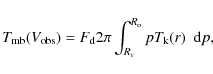
The characteristic brightness of a source (neglecting the cosmic background, whose temperature is much lower than
|
(7) |
Where S, the source function, depends on the frequency much less sharply than the line profile:
|
(8) |
Since we are assuming that the populations are thermalized (Eqs. (1), (2)) and, again, that
|
(9) |
Leading to the usual equations for the optically thick case,
| (10) |
and for the optically thin case,
| (11) |
Equation (10) holds for the range of velocities around the systemic one for which the opacity is still higher than 1 and
From these equations we can also deduce the dependence of ![]() on
on ![]() ,
in particular taking into account the dependence of
,
in particular taking into account the dependence of
![]() on
on ![]() (see Eq. (4)):
(see Eq. (4)): ![]()
![]()
![]() in the optically thick case and
in the optically thick case and ![]()
![]() 1/
1/![]() in
the optically thin case.
in
the optically thin case.
Finally, for a source with a typical size L, in arcsecond units,
observed with a telescope beam with typical half-power beam width equal
to ![]() ,
also in arcseconds,
the main beam temperature
,
also in arcseconds,
the main beam temperature
![]() (over the cosmic background)
will be
(over the cosmic background)
will be
|
(12) |
(We are assuming that the typical source size L represents the source observable diameter at half-maximum, and that the dilution factor within the beam,
3.2 Line shapes: optically thin emission
The typical profiles of molecular lines from CSEs around standard AGB stars, very extended and expanding at supersonic almost constant velocities, are well known. Parabolic, flat-topped or two-horn profiles are expected depending on whether the lines are optically thin or thick and on whether the source is spatially resolved by the telescope (e.g., Olofsson et al. 1982).
The profile shapes are of course modified by the presence of
significant local velocity dispersions, which yield profiles that are
in some way the convolution of the above prototypes with the local
distribution (often assumed to be described by a Gaussian function). A
discussion of the line formation when the local velocity dispersion is
not negligible requires detailed computations. Therefore, we assume
in this section that the turbulence velocity is much lower than the
macroscopic velocity field (which is very often the case in CSEs
around AGB stars, with expansion velocities
around 10 km s-1 and local dispersions ![]() 1 km s-1).
1 km s-1).
In the very inner circumstellar shells we do not expect such constant outward velocities. When significant acceleration is still present, simple sharply-peaked profiles are expected; see the general discussion and comparison with standard profiles in Bujarrabal et al. (1989).
Simple considerations can yield analytical insight into the expected
profiles from these regions. We recall that, in our sources, we can
assume spherical symmetry and isotropic expansion, thermalized
populations,
![]() ,
unresolved sources, and a constant
abundance.
,
unresolved sources, and a constant
abundance.
In the optically thin case, the velocity-integrated emission in a
certain CO line of a certain mass of gas M at a temperature ![]() is just proportional to
is just proportional to
![]() (from Eqs. (3) to
(12)). Therefore, the brightness temperature emitted by a geometrically
thin shell (radius: r) integrated over observable velocities,
(from Eqs. (3) to
(12)). Therefore, the brightness temperature emitted by a geometrically
thin shell (radius: r) integrated over observable velocities,
![]() (projected on a line of sight), would be
(projected on a line of sight), would be
|
(13) |
Some obvious geometrical considerations show that the brightness,
If we assume a constant mass-loss rate, ![]() ,
n(r)
,
n(r) ![]()
![]() /r2/V(r), and
/r2/V(r), and
|
(14) |
The total emission of the optically thin envelope, between its inner and outer radii,
|
(15) |
Where the integral extends only to shells such that
If we assume, for instance, a constant increase in V with r,
![]() ,
and constant
,
and constant ![]() ,
the variation
of
,
the variation
of
![]() with
with
![]() from Eq. (15) becomes
from Eq. (15) becomes
|
(16) |
Except for truncation for central velocities such that
If ![]() varies like 1/r, the solution is also sharply peaked:
varies like 1/r, the solution is also sharply peaked:
|
(17) |
for
Finally, we recall that the conversion of the proportionality relations
given here into true equations (i.e. the substitution of ![]() for
=) is straightforward using the complete expression for
for
=) is straightforward using the complete expression for ![]() as given
in Eq. (3).
as given
in Eq. (3).
3.3 Line shapes: optically thick emission
As in Sect. 3.2, our model CSE presents spherical symmetry and
isotropic expansion. Let us now assume that the emission from a
geometrically thin shell within a velocity range,
![]() ,
centered on the systemic velocity
,
centered on the systemic velocity
![]() ,
is optically
thick. In general,
,
is optically
thick. In general,
![]() /2 can be assumed to be equal to
the maximum expansion velocity in the CSE. The corresponding main-beam
temperature is then just proportional to the kinetic temperature,
/2 can be assumed to be equal to
the maximum expansion velocity in the CSE. The corresponding main-beam
temperature is then just proportional to the kinetic temperature,
![]() ,
and to the solid angle from which emission at this
velocity is emitted (Sect. 3.1). We also assume that the expansion
velocity V(r) is constant or monotonically increasing with the
distance to the center, in order to simplify the formulae, and again a
small local velocity dispersion. Also for the sake of simplicity in
formulae, we assume that
,
and to the solid angle from which emission at this
velocity is emitted (Sect. 3.1). We also assume that the expansion
velocity V(r) is constant or monotonically increasing with the
distance to the center, in order to simplify the formulae, and again a
small local velocity dispersion. Also for the sake of simplicity in
formulae, we assume that
![]() = 0; in other words, our
observed velocity
= 0; in other words, our
observed velocity
![]() is considered in this subsection to be
measured with respect to the characteristic velocity of the source.
is considered in this subsection to be
measured with respect to the characteristic velocity of the source.
The total emission in main-beam temperature units of the circumstellar
envelope (with inner and outer radii ![]() and
and ![]() ),
within
),
within ![]()
![]() (i.e. within
(i.e. within
![]()
![]()
![]() ), is then
), is then
|
(18) |
where Rv is the minimum radius emitting at
|
(19) |
Therefore, the main-beam brightness temperature in the optically thick case is given by
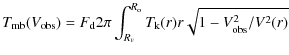
|
|||
![$\displaystyle \times\left[ \frac{V(r) - r V'(r)}{V^2(r)} \sqrt{V^2(r)-V^2_{\rm ...
...rac{r}{V(r)} \frac{V(r)V'(r)}{\sqrt{V^2(r) - V^2_{\rm obs}}} \right]
~{\rm d}r.$](/articles/aa/full_html/2010/08/aa13743-09/img85.png)
|
(20) |
These equations systematically lead to profiles with a central peak, but less sharp than in the optically thin case. For instance, if the expansion velocity is constant,
|
(21) |
In the case of a constant velocity gradient, V(r) =
|
(22) |
For the assumed velocity field,
For constant ![]() ,
parabolic profiles are again predicted:
,
parabolic profiles are again predicted:
![]()
![]() ,
assuming very small
,
assuming very small ![]() (otherwise the profiles are
parabolic except for truncation in the central velocities).
It is, however, more realistic to assume that the temperature decreases
outwards, which leads to more sharply peaked shapes. If, for instance,
(otherwise the profiles are
parabolic except for truncation in the central velocities).
It is, however, more realistic to assume that the temperature decreases
outwards, which leads to more sharply peaked shapes. If, for instance,
![]() [and, we recall,
[and, we recall,
![]() ], we get from Eq. (22) sharp
profiles that are exactly triangular if
], we get from Eq. (22) sharp
profiles that are exactly triangular if ![]()
![]()
![]() :
:
![\begin{displaymath}T_{\rm mb}(V_{\rm obs}) = F_{\rm d} 2 \pi T_{\rm k}(R_{\rm o}...
...1 - \frac{\vert V_{\rm obs}\vert}{V(R_{\rm o})} \right] \cdot
\end{displaymath}](/articles/aa/full_html/2010/08/aa13743-09/img100.png)
|
(23) |
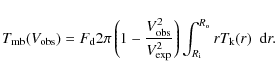
When the temperature decreases linearly from
| |
= | ![$\displaystyle F_{\rm d} \pi R^2_{\rm o} T_{\rm k}(R_{\rm i}) [1 - V^2_{\rm obs}/V^2(R_{\rm o})]$](/articles/aa/full_html/2010/08/aa13743-09/img103.png)
|
|
![$\displaystyle -\frac{2}{3}
F_{\rm d} \pi [T_{\rm k}(R_{\rm i}) - T_{\rm k}(R_{\rm o})] [1 - \vert V_{\rm obs}\vert^3/V^3(R_{\rm o})].$](/articles/aa/full_html/2010/08/aa13743-09/img104.png)
|
(24) |
In this case, the profile is more sharply peaked than the parabolic profile obtained for constant
These equations are particularly interesting for us, because probably the kinetics of the circumstellar shells in our sources shows a significant velocity gradient and our 12CO lines are optically thick. We therefore expect more or less triangular profiles with a central peak. As we will see below, other phenomena should also be considered to explain the asymmetry in the observed profiles.
3.3.1 Selfabsorption in optically thick envelopes
In discussion in Sects. 3.2 and 3.3, we have assumed that the local
velocity dispersion, presumably caused by turbulent movements, is much
smaller than the macroscopic velocities. A variety of line profiles
were found, but, in particular, in all cases the profiles were
symmetric around the systemic velocity
![]() .
If the local
velocity dispersion is not negligible (and the temperature is not
constant), selfabsorption must be taken into account. In the most usual
case, in which the temperature decreases outwards, selfabsorption is
important for the most negative velocities (gas approaching the
observer), since then outer cool regions absorb the emission of hotter,
inner regions. This is not the case for the positive velocities, in
which the hotter regions would be closer to the observer, its emission
dominating the observed line. The result is an asymmetric profile in
which the maximum is shifted to positive velocities, while keeping the
total emission range.
.
If the local
velocity dispersion is not negligible (and the temperature is not
constant), selfabsorption must be taken into account. In the most usual
case, in which the temperature decreases outwards, selfabsorption is
important for the most negative velocities (gas approaching the
observer), since then outer cool regions absorb the emission of hotter,
inner regions. This is not the case for the positive velocities, in
which the hotter regions would be closer to the observer, its emission
dominating the observed line. The result is an asymmetric profile in
which the maximum is shifted to positive velocities, while keeping the
total emission range.
Unfortunately, these effects are too complex to be discussed by means of analytical, simple formulae, such as those given before, and numerical calculations must be performed. In Sect. 3.4 we present a numerical model that takes selfabsorption into account, within an accurate description of radiative transfer in expanding envelopes. We also see in Sect. 4 how these phenomena are useful to better understand our observations of SSs, particularly the asymmetric profile of the J=2-1 line observed in R Aqr.
3.4 Numerical model of line formation
We used a numerical model to simulate the line formation in our case similar to that described by Teyssier et al. (2006), adapted to the high densities and temperatures expected in the inner circumstellar shells. See more details on the numerical code in that paper.
In the calculation of the level population, we have taken collisional and radiative excitation into account, considering a high number of rotational levels in two vibrational states. Our calculations confirm that, as shown in Sect. 3.1, the population of all relevant levels is very accurately thermalized because of the expected high densities. Therefore, our results practically do not depend on the details of the treatment of the excitation. The radiative transfer equation is accurately solved taking a local turbulence velocity and the macroscopic velocity field into account. We thus calculate the brightness in the direction to the observer along a number of lines of sight and for a number of projected velocities. These results are convolved with the beam shape assumed for the observed lines, obtaining a Rayleigh-Jeans-equivalent main-beam temperature for a number of LSR velocities, directly comparable to the observed profiles. Thanks to the small extent of the source, this convolution practically does not depend on the exact beam shape, so the beam width is the only relevant parameter in the calculation.
In this model, we are assuming that the emitting region is spherical
and expands isotropically. We also assume that the physical and
chemical conditions are in our case similar to those typical of inner
shells around standard AGB stars. This may be not true in symbiotic
systems, whose inner circumstellar layers could present an axis of
symmetry, anomalous density and velocity distributions, and other
peculiar properties. We think that our lack of knowledge on these
probably complex regions (from molecular line observations or from
other studies) prevents more detailed modeling. Observations of SiO
maser emission in R Aqr (e.g. Cotton et al. 2004; Pardo et al. 2004; Kamohara et al. 2010)
show properties completely similar to those found in standard AGB
stars. VLBI maps show, in particular, that the SiO maser in general
occupy a ring-like region (with radius
![]() cm) that is
comparable to those typical of AGB stars. Kamohara et al. find that
the spatial distribution, nevertheless, tends to show a certain axial
symmetry. The departures from spherical symmetry do not always show the
same pattern and are in many epochs quite small, but the axis
orientation has remained stable at a position angle of about
-10
cm) that is
comparable to those typical of AGB stars. Kamohara et al. find that
the spatial distribution, nevertheless, tends to show a certain axial
symmetry. The departures from spherical symmetry do not always show the
same pattern and are in many epochs quite small, but the axis
orientation has remained stable at a position angle of about
-10![]() during more than 10 years. The SiO data therefore indicate
that the inner shells around R Aqr are more or less spherical and,
because SiO masers are excited normally, must show physical conditions
similar to those usually present in AGB stars; at least up to a
distance of about
during more than 10 years. The SiO data therefore indicate
that the inner shells around R Aqr are more or less spherical and,
because SiO masers are excited normally, must show physical conditions
similar to those usually present in AGB stars; at least up to a
distance of about
![]() cm, i.e. in regions not much smaller that
the total region assumed to be responsible for the CO lines in our
model.
cm, i.e. in regions not much smaller that
the total region assumed to be responsible for the CO lines in our
model.
4 Results
We have detected 12CO J=2-1 and J=1-0 emission from the symbiotic stellar systems (SSs) R Aqr and CH Cyg (the detection of J=1-0 in R Aqr being tentative). We also present limits to the emission of 12CO J=2-1 and J=1-0 in another SS, HM Sge, and to the emission of 13CO J=2-1 and J=1-0 and SiO J=5-4 in R Aqr. A summary of our observational results can be seen in Table 1 and the detected lines are shown in Figs. 1, 2. We can interpret these data by means of the relatively simple formulation presented in Sects. 3.1-3.3, but some observational features require numerical calculations, using the code presented in Sect. 3.4. We see that the observations are explained reasonably well by those predictions, and other cases that do not seem compatible with our data, like the narrow two-horn profiles from rotating disks, will not be considered.
Table 1: Summary of observational results.
![\begin{figure}
\par\includegraphics[angle=270,width=9cm,clip]{13743fg2.eps}
\end{figure}](/articles/aa/full_html/2010/08/aa13743-09/img107.png)
|
Figure 2: 12CO lines detected in CH Cyg. |
| Open with DEXTER | |
4.1 CO lines in R Aqr
Let us apply the simple formulae in Sect. 3 to our observations of CO
in R Aqr. We first assume that the radius of the emitting region
is smaller than the component separation, i.e., that ![]()
![]() 09 (
09 (
![]() cm at a distance of 214 pc). Then, the upper
limit to the antenna temperature is given by the optically thick case
emission:
cm at a distance of 214 pc). Then, the upper
limit to the antenna temperature is given by the optically thick case
emission:
![]() (12COJ=2-1)
(12COJ=2-1) ![]()
![]() K. The observed intensity in R Aqr implies a typical kinetic
temperature of about 500 K. Slightly higher temperatures will be
derived if the line opacity is not extremely high, which, as we will
argue below, is probably the case. From Eq. (3), Sect. 3.1, and
assuming a CO abundance of about
K. The observed intensity in R Aqr implies a typical kinetic
temperature of about 500 K. Slightly higher temperatures will be
derived if the line opacity is not extremely high, which, as we will
argue below, is probably the case. From Eq. (3), Sect. 3.1, and
assuming a CO abundance of about
![]() ,
typical in CSEs
around O-rich Mira-type stars, we deduce that the assumption of
optically thick 12CO J=2-1 emission implies densities
,
typical in CSEs
around O-rich Mira-type stars, we deduce that the assumption of
optically thick 12CO J=2-1 emission implies densities
![]() cm-3. As we have discussed in Sect. 1, both deduced values of the
temperature and density agree with current expectations for the
innermost shells around AGB stars.
cm-3. As we have discussed in Sect. 1, both deduced values of the
temperature and density agree with current expectations for the
innermost shells around AGB stars.
We discussed the expected line ratios in our case in Sect. 3.1,
Eqs. (6), (10), (11), and (12). In the completely opaque case, the intensity
ratio of the J=2-1 and J=1-0 lines must be
![]() (J=2-1)/
(J=2-1)/
![]() (J=1-0)
(J=1-0) ![]()
![]() (J=1-0)/
(J=1-0)/
![]() (J=2-1)
(J=2-1) ![]() 3.5. In the fully optically thin case,
3.5. In the fully optically thin case,
![]() (2-1)/
(2-1)/
![]() (1-0)
(1-0) ![]()
![]() (2-1)/
(2-1)/![]() (1-0)
(1-0) ![]()
![]() (1-0)/
(1-0)/
![]() (2-1) = 4
(2-1) = 4
![]() (1-0)/
(1-0)/
![]() (2-1)
(2-1) ![]() 14. The line
14. The line
![]() ratio is
ratio is ![]() 6 (if we
believe that our CO J=1-0 line is detected,
6 (if we
believe that our CO J=1-0 line is detected, ![]() 6 otherwise; in any
case, the uncertainty is very large). Therefore, our observations
suggest that the CO J=1-0 line in this source is moderately optically
thin, typical values of
6 otherwise; in any
case, the uncertainty is very large). Therefore, our observations
suggest that the CO J=1-0 line in this source is moderately optically
thin, typical values of ![]() (J=1-0)
(J=1-0) ![]() 0.8-1 are enough to
explain the (tentatively) measured line ratio. Since the typical
0.8-1 are enough to
explain the (tentatively) measured line ratio. Since the typical ![]() ratio is
ratio is ![]() (J=2-1)/
(J=2-1)/![]() (J=1-0)
(J=1-0) ![]() 4, the J=2-1 line would be in
any case opaque. These values of
4, the J=2-1 line would be in
any case opaque. These values of ![]() (J=1-0) imply densities
(J=1-0) imply densities ![]() 109 cm-3 (from formulae in Sect. 3.1), very reasonable in this
context. The total mass in the emitting shell is therefore deduced to
be
109 cm-3 (from formulae in Sect. 3.1), very reasonable in this
context. The total mass in the emitting shell is therefore deduced to
be
![]()
![]() .
.
Other possibilities that could explain the observations are much less
probable. A significantly larger extent would imply temperature almost
decreasing with 1/L2, to keep the observed intensity of the J=2-1 line. For instance,
![]() cm would imply an average
temperature of
cm would imply an average
temperature of ![]() 45 K within the emitting region, surprisingly
low for shells around Mira-type stars (mostly taking the presence of a
hot companion into account). Values of L as low as
45 K within the emitting region, surprisingly
low for shells around Mira-type stars (mostly taking the presence of a
hot companion into account). Values of L as low as
![]() 1014 cm would imply typical temperatures of about 5000 K,
even higher than the surface temperature of the cool star.
These predictions of intensity, deduced from a simple but robust line
formation model, have been fully confirmed by computations performed
with the model presented in Sect. 3.4. (Calculations performed
with this code will be discussed in more detail below.)
1014 cm would imply typical temperatures of about 5000 K,
even higher than the surface temperature of the cool star.
These predictions of intensity, deduced from a simple but robust line
formation model, have been fully confirmed by computations performed
with the model presented in Sect. 3.4. (Calculations performed
with this code will be discussed in more detail below.)
The shape of our 12CO J=2-1 profile is clearly different from the wide profiles observed in the extended envelopes around standard AGB stars (parabolic, flat-topped or two-horned). The profile, which shows a relatively sharp central peak, is compatible with the expected profile for the compact, very small shells expected in SSs (Sects. 3.2, 3.3), in which a significant acceleration of the gas is expected to be present.
Therefore, both the intensity of the CO J=2-1 and J=1-0 lines and the
shape of J=2-1 are compatible with our expectations for the CO
emission in circumstellar regions closer than about
![]() cm.
cm.
To better understand the properties of the emitting region and check the above conclusions, we tried to fit our CO observations of R Aqr with the predictions of the numerical line formation model presented in Sect. 3.4. We must keep in mind that the source modeling and the determination of the properties of this shell can only be a first step in the study of these layers, because of the lack of information on them, including, in particular, the poor data on molecular emission. Moreover, in the inner circumstellar shells around the cool component of an interacting binary system, we can expect complex structures and velocity fields, perhaps difficult to compare with the smooth, continuous ejection of material by standard AGB stars, and yielding line shapes with features that cannot be accounted for by our simple shell model. The best we can do is to find a set of characteristic properties of the emitting region, namely, extent, velocity field, and physical conditions, that yield predicted line profiles compatible with the observations.
![\begin{figure}
\par\includegraphics[angle=270,width=9cm,clip]{13743fg3.ps}
\end{figure}](/articles/aa/full_html/2010/08/aa13743-09/img119.png)
|
Figure 3: Distributions of the expansion velocity and kinetic temperature (red dashed line) deduced from our simple modelization of the CO-rich, inner shells around R Aqr. |
| Open with DEXTER | |
The envelope extent is defined by its inner and outer radii, ![]() ,
,
![]() .
We imposed a low value of
.
We imposed a low value of ![]() ,
slightly higher than the stellar radius, and a value of
,
slightly higher than the stellar radius, and a value of ![]() equal to
equal to
![]() cm, to agree with general
considerations discussed above. We assumed that the velocity,
V(r), increases from a certain point in the inner envelope (supposed
to be related to dust formation).
We assume a turbulence velocity comparable to the minimum expansion
velocity,
cm, to agree with general
considerations discussed above. We assumed that the velocity,
V(r), increases from a certain point in the inner envelope (supposed
to be related to dust formation).
We assume a turbulence velocity comparable to the minimum expansion
velocity,
![]() .
The temperature is assumed to vary linearly
in the considered region, between
.
The temperature is assumed to vary linearly
in the considered region, between
![]() and
and
![]() ,
and the density varies assuming a constant mass-loss
rate,
,
and the density varies assuming a constant mass-loss
rate, ![]() ,
i.e.:
,
i.e.:
![]() .
For both
the kinetic temperature and the expansion velocity, only linear
functions are considered, in view of our poor knowledge on these
parameters in SSs. The CO abundance, X(CO), is assumed to be
constant and equal to
.
For both
the kinetic temperature and the expansion velocity, only linear
functions are considered, in view of our poor knowledge on these
parameters in SSs. The CO abundance, X(CO), is assumed to be
constant and equal to
![]() ,
a typical value in CSEs
around O-rich AGB stars. Since the level population is
practically thermalized, we can vary the value of X(CO) and obtain
practically the same results, provided that the density varies in the
opposite sense and the product
,
a typical value in CSEs
around O-rich AGB stars. Since the level population is
practically thermalized, we can vary the value of X(CO) and obtain
practically the same results, provided that the density varies in the
opposite sense and the product
![]() remains constant.
remains constant.
![\begin{figure}
\par\includegraphics[angle=270,width=9cm,clip]{13743fg4.ps}\vspace*{-2mm}
\end{figure}](/articles/aa/full_html/2010/08/aa13743-09/img124.png)
|
Figure 4: 12CO J=2-1 profile predicted by our best-fit model of the inner shells around R Aqr, red dashed line, superimposed on our observed profile. |
| Open with DEXTER | |
We have found a set of values for the above parameters that can explain
the observations. The temperature and velocity laws are given in Fig. 3. In the outer shells around standard AGB stars the
velocity gradient becomes very small and the expansion velocity
increases slowly up to a certain asymptotic value, but this regime
apparently is not reached in the compact shells around R Aqr we are
describing here. The best-fit value of the mass-loss rate is
![]()
![]() yr-1. In Fig. 4 we show the predicted profile, superimposed
to the observed one.
yr-1. In Fig. 4 we show the predicted profile, superimposed
to the observed one.
Because of the poor observational data on 12CO J=1-0, we have not
tried to fit the observed profiles, but we checked that the
predicted intensity,
![]()
![]() 5 mK, is compatible with the
observation.
5 mK, is compatible with the
observation.
The asymmetric line shape, with a slightly red-shifted maximum, is reproduced well by our model, due to absorption of the emission of inner shells by the cooler outer regions, only noticeable at relatively negative velocities (Sect. 3.3.1). The expansion velocity (a parameter almost directly given by the observed profile width) is also quite high, compared to other AGB shells, compatible with the idea that mass ejection is particularly efficient in SSs (Sect. 1).
Given the lack of information about the emitting region and the
relatively simple model we are using, it is obvious that the values
deduced here for the different parameters are indicative and relatively
uncertain. Nevertheless, we think that our being able to reasonably fit
the observations shows that our basic assumptions about the emitting
region (size, temperature and velocity ranges, densities, etc.) are
essentially correct. This conclusion is supported by observational
results of SiO maser emission in this object, see Sect. 3.4, which
suggest that inner shells around R Aqr (not much smaller than our CO
emitting region) are more or less spherical and show physical
conditions similar to those typical in AGB stars. On the other hand,
moderately oblate density distributions have been proposed for the
inner circumstellar regions in SSs (Gawryszczak et al. 2002; Podsiadlowski & Mohamed 2007), as caused by
gravitational focusing. From the existing data, we cannot distinguish
between these oblate distributions and more spherical ones. Since the
binary orbit in R Aqr is nearly edge-on, the assumption of such an
oblate structure would limit our requirements of relatively high column
densities to its equator. Therefore, the values of the mass-loss rates
for R Aqr would be, in this case, somewhat less than those given above,
and we would deduce lower values for ![]() by a factor of
by a factor of ![]() 2. A
similarly lower value of the mass-loss rate can be obtained, in
general, if we allow the radius of the spherical shell to increase
moderately, for instance, up to the separation between the stars, 2.3-
2. A
similarly lower value of the mass-loss rate can be obtained, in
general, if we allow the radius of the spherical shell to increase
moderately, for instance, up to the separation between the stars, 2.3-
![]() cm. The data could be also reproduced assuming the
source to be somewhat smaller than in our standard model, higher values
of the gas temperature and the mass-loss rate then being
deduced. (Stronger variations in the source size would lead to
unexpected properties of the emitting gas, as mentioned before.) Strong
variations in the total mass and mass-loss rate in the case of a
significantly clumpy medium are also improbable, provided that the
total size does not vary a lot, because the typical opacity and column
density required to explain the observations would not change.
cm. The data could be also reproduced assuming the
source to be somewhat smaller than in our standard model, higher values
of the gas temperature and the mass-loss rate then being
deduced. (Stronger variations in the source size would lead to
unexpected properties of the emitting gas, as mentioned before.) Strong
variations in the total mass and mass-loss rate in the case of a
significantly clumpy medium are also improbable, provided that the
total size does not vary a lot, because the typical opacity and column
density required to explain the observations would not change.
Published estimates of the mass-loss rates from the Mira component of R
Aqr (and in general for symbiotic Miras) are based either on radio
continuum observations or on FIR IRAS data
(e.g. Kenyon et al. 1988; Seaquist & Taylor 1990). The former method probes the
ionized portion of the wind, whereas the latter measures the amount of
dust in the system. In particular, Seaquist & Taylor (1990) estimated a
mass-loss rate from the Mira of
![]()
![]() yr-1 from 6 cm
radio flux, which would become
yr-1 from 6 cm
radio flux, which would become
![]()
![]() yr-1 for the distance value
adopted here and an expansion velocity
yr-1 for the distance value
adopted here and an expansion velocity
![]() km s-1.
(There is a typing error in Table IV of Kenyon et al. 1988. They
should give the same value for the gas mass-loss rate as Seaquist &
Taylor because both papers used the same data.)
km s-1.
(There is a typing error in Table IV of Kenyon et al. 1988. They
should give the same value for the gas mass-loss rate as Seaquist &
Taylor because both papers used the same data.)
The IRAS data for symbiotic stars were analyzed by Anandarao & Pottasch (1986),
Anandarao et al. (1988), and Kenyon et al. (1988). The first group, based on
analysis of the IRAS LRS data and the broad-band IRAS photometry, found
two dust shells in R Aqr: a hotter inner shell with a temperature of
about 800 K, a radius of about 6 AU or
![]() cm (assuming
cm (assuming
![]() pc), and a dust mass of
pc), and a dust mass of
![]()
![]() ,
which may overlap with the CO region, and an outer cold shell with
about 87 K, a radius of about 123 AU, and a mass of
,
which may overlap with the CO region, and an outer cold shell with
about 87 K, a radius of about 123 AU, and a mass of
![]()
![]() .
The hot inner shell alone can account for the LRS
fluxes, whereas the second outer shell explains the far-IR fluxes,
mainly in the 60 and 100 micron IRAS bands. A similarly complex dust
structure was found in all of seven studied symbiotic systems and was
interpreted as a signature of multiple circumstellar shells because of
a discontinuous mass distribution. Anandarao et al. (1988) also suggested
that the inner shells represent the basic envelopes of the cool
components, whereas the outer shells are circumbinary components. If
the inner shells indeed result from the present mass ejection by the
Mira, this value of dust mass requires a mass-loss rate of about
10-5
.
The hot inner shell alone can account for the LRS
fluxes, whereas the second outer shell explains the far-IR fluxes,
mainly in the 60 and 100 micron IRAS bands. A similarly complex dust
structure was found in all of seven studied symbiotic systems and was
interpreted as a signature of multiple circumstellar shells because of
a discontinuous mass distribution. Anandarao et al. (1988) also suggested
that the inner shells represent the basic envelopes of the cool
components, whereas the outer shells are circumbinary components. If
the inner shells indeed result from the present mass ejection by the
Mira, this value of dust mass requires a mass-loss rate of about
10-5 ![]() yr-1 (assuming gas/dust mass ratio
yr-1 (assuming gas/dust mass ratio ![]() 100 and
100 and
![]() km s-1), in good agreement with our estimate based on CO
line emission.
km s-1), in good agreement with our estimate based on CO
line emission.
On the other hand, the dust shell parameters derived from broad-band
IRAS photometry by Kenyon et al. (1988), temperature ![]() 450 K and radius
of
450 K and radius
of ![]() 70 AU, are significantly different from the above values, and
they are indeed incompatible with the LRS data. Their dust shell mass,
70 AU, are significantly different from the above values, and
they are indeed incompatible with the LRS data. Their dust shell mass,
![]()
![]() (recalculated for our distance), is
similar to the mass of the inner shell proposed by Anandarao et al.;
but, owingo the larger extent of the shell, the mass-loss rate is
(recalculated for our distance), is
similar to the mass of the inner shell proposed by Anandarao et al.;
but, owingo the larger extent of the shell, the mass-loss rate is
![]()
![]() yr-1 (assuming gas/dust mass ratio
yr-1 (assuming gas/dust mass ratio ![]() 100, and
100, and
![]() km s-1), an order of magnitude
lower than our CO-based estimate. Finally, Gromadzki et al. (2009) derive
a mass-loss rate
km s-1), an order of magnitude
lower than our CO-based estimate. Finally, Gromadzki et al. (2009) derive
a mass-loss rate ![]()
![]() 10-6
10-6 ![]() yr-1 for R Aqr, from
the K-[12] color versus
yr-1 for R Aqr, from
the K-[12] color versus ![]() relation calibrated for normal AGB
stars, but its extrapolation to our case is uncertain.
relation calibrated for normal AGB
stars, but its extrapolation to our case is uncertain.
In general, the comparison between the mass-loss rates derived from dust and molecular line emissions in R Aqr is very uncertain, because the interpretation of both molecular and FIR data under our extreme conditions is not standard and because the dust-to-gas ratio may be significantly different in shells around SSs and in standard AGB stars. The dust content in the molecule-rich shells in symbiotic systems may be lower than in CSEs around normal evolved stars, because we only detect CO line emission from very inner shells in which grains are not yet completely formed, as in fact suggested by the strong velocity gradient deduced from our modelization. On the other hand, it is clear that grains can survive the radiation from the hot companion much more easily, therefore we could detect dust emission from regions in which molecules do not exist.
The comparison of results on ionized and molecular gas also needs to be discussed. The high-density gas is, in general, much harder to ionize and photodissociate by the hot companion because of self-shielding. We have mentioned that hydrodynamical numerical simulations show that flows from the Mira in SSs can be concentrated towards the orbital plane, resulting in a large-scale density enhancement in the orbital plane and low-density polar regions (see e.g. Gawryszczak et al. 2002, and references therein). One can then expect the molecular material (and to a lesser extent the dust) to be placed near the orbital plane, as well as the presence of two ionized regions in the poles (and probably outside the orbit). The methods based on observations of molecular gas and dust would refer to the denser material, probably lying close to the orbital plane, whereas the radio continuum data would probe the low-mass regions. As a result, one should get higher mass values from molecular lines and dust than from radio continuum data. Our rates from CO are about 2 orders of magnitude higher than published values based on radio data, in agreement with these expectations.
4.2 CO lines in CH Cyg
The poor 12CO profiles observed in CH Cyg prevent any detailed
fitting of the line shape. Both lines roughly show a central peak and
could be compatible with the emission of a region with significant
velocity gradient. We can derive some characteristics of the emitting
region from the line intensity. First of all, we can see that the
J=2-1/J=1-0 intensity ratio is relatively high, compatible with the
optically thick ratio, ![]() 3.5 (Sect. 3.1; see also discussion for
R Aqr in 4.1). We also note that the component separation in the object
is
3.5 (Sect. 3.1; see also discussion for
R Aqr in 4.1). We also note that the component separation in the object
is ![]() 9 AU, less than for R Aqr. Therefore we can assume that both
lines are optically thick and both come from a very compact
region. From our discussion in Sect. 3.1, we can deduce that the
observed line intensities are compatible with an emitting region size
(typical diameter) of about 10 AU (typical radius
9 AU, less than for R Aqr. Therefore we can assume that both
lines are optically thick and both come from a very compact
region. From our discussion in Sect. 3.1, we can deduce that the
observed line intensities are compatible with an emitting region size
(typical diameter) of about 10 AU (typical radius ![]() 5 AU, somewhat
smaller than the component separation), and a typical kinetic temperature
of about 800 K. We stress that, because of the lack of good CO
profiles in this source, the assumption that the emission comes from a
small shell in expansion is less well founded than for R Aqr. This
uncertainty and the low S/N obviously result in less accurate
conclusions from the data.
5 AU, somewhat
smaller than the component separation), and a typical kinetic temperature
of about 800 K. We stress that, because of the lack of good CO
profiles in this source, the assumption that the emission comes from a
small shell in expansion is less well founded than for R Aqr. This
uncertainty and the low S/N obviously result in less accurate
conclusions from the data.
The detected profiles are, within the uncertainties, quite wide,
suggesting that high expansion velocities are present in the CO-rich
shells, ![]() 25 km s-1, even higher than those measured for R Aqr. The
mass-loss rates must also be quite high, also larger than for R Aqr, to
take the larger opacities and velocity dispersion into account (the
velocity dispersion enters both in the opacity, Eq. (4), and in the
estimate of the shell lifetime). We deduce, following the prescriptions
in Sect. 3.1,
25 km s-1, even higher than those measured for R Aqr. The
mass-loss rates must also be quite high, also larger than for R Aqr, to
take the larger opacities and velocity dispersion into account (the
velocity dispersion enters both in the opacity, Eq. (4), and in the
estimate of the shell lifetime). We deduce, following the prescriptions
in Sect. 3.1, ![]()
![]()
![]()
![]() yr-1. We suggest that the
high values of the mass-loss rate and expansion velocity are partially
caused by the CH Cyg system being tighter than that of R Aqr.
yr-1. We suggest that the
high values of the mass-loss rate and expansion velocity are partially
caused by the CH Cyg system being tighter than that of R Aqr.
The high mass-loss rate in CH Cyg may be surprising, in particular
because it is a semiregular (SR) variable, and it is well known that SR
variables in general show significantly lower mass-loss rates than
Mira-type variables. However, the case of CH Cyg is peculiar. CH Cyg
presents a complex variation pattern that probably includes two
periods of about 100 and 760 days, plus other long-term variations,
with a high overall variability amplitude, about 3 mag in the visible;
see the light curve by the AAVSO and Mikoajewski et al. (1992).
Miko![]() ajewski et al. indeed classify this source as SRa variable. The
basic properties and evolutionary status of the SR variables of type
SRa and SRb were comprehensively discussed by
Kerschbaum & Hron (1996,1992,1994), who find that SRa stars appear as
intermediate objects between Miras and SRb variables in all aspects,
including periods, amplitudes, and mass-loss rates. Gromadzki et al. (2007) find that most giants in symbiotic systems reveal more or
less regular pulsations with periods in the range 50-400 days. They
also conclude that the presence of such variability can account for
the relatively high mass-loss rates usually found in symbiotic stars as
compared with single field giants (Sects. 1, 5).
ajewski et al. indeed classify this source as SRa variable. The
basic properties and evolutionary status of the SR variables of type
SRa and SRb were comprehensively discussed by
Kerschbaum & Hron (1996,1992,1994), who find that SRa stars appear as
intermediate objects between Miras and SRb variables in all aspects,
including periods, amplitudes, and mass-loss rates. Gromadzki et al. (2007) find that most giants in symbiotic systems reveal more or
less regular pulsations with periods in the range 50-400 days. They
also conclude that the presence of such variability can account for
the relatively high mass-loss rates usually found in symbiotic stars as
compared with single field giants (Sects. 1, 5).
It is also remarkable that semiregular variables with amplitudes ![]() 2.5 mag (like W Hya, GY Aql, T Ari, etc.) tend to present strong SiO
maser emission, comparable to that of standard Miras
(Alcolea et al. 1990). Therefore, the density and general physical
conditions in the inner circumstellar layers should not differ
significantly from those of Mira-type variables. These and some other SR
stars (W Hya, GY Aql, RX Boo, EP Aqr, X Her, etc.) show dense extended
envelopes detected in CO. It is also well known that a number of
SRs (EP Aqr, RX Boo, X Her, RS Cnc, etc) show extended shells with a
clear axis of symmetry (e.g. Nakashima 2005), similar to those
found in Mira-type stars in binary systems, such as o Cet and V Hya
(e.g. Kahane et al. 1996).
2.5 mag (like W Hya, GY Aql, T Ari, etc.) tend to present strong SiO
maser emission, comparable to that of standard Miras
(Alcolea et al. 1990). Therefore, the density and general physical
conditions in the inner circumstellar layers should not differ
significantly from those of Mira-type variables. These and some other SR
stars (W Hya, GY Aql, RX Boo, EP Aqr, X Her, etc.) show dense extended
envelopes detected in CO. It is also well known that a number of
SRs (EP Aqr, RX Boo, X Her, RS Cnc, etc) show extended shells with a
clear axis of symmetry (e.g. Nakashima 2005), similar to those
found in Mira-type stars in binary systems, such as o Cet and V Hya
(e.g. Kahane et al. 1996).
On the other hand, it is obvious from our discussion in Sects. 4.1 and 5 that the mass ejection by the evolved component of an SS can be seriously affected by the stellar interaction, and we have seen that mass-loss rates in such systems tend to be higher than in isolated AGB stars (Sects. 1, 5). It is then to be expected that the interacting nature of the CH Cyg system strongly affects the structure, dynamics, and density of the inner circumstellar layers, helping to understand the measured high amount of gas in these regions.
The presence of a relatively high amount of mass in the inner circumstellar shells of CH Cyg is confirmed by its FIR dust emission and by the identification of a hot dust shell, a few times larger than the stellar photosphere, which significantly contributes to the total NIR flux (Pedretti et al. 2009). The values derived here for the mass-loss rate and typical temperature in the inner shells are quite similar to those found by Taranova & Shenavrin (2007) from analysis of the dust FIR emission of recently ejected material. Our mass-loss rates are also compatible with the total dust mass derived by Kenyon et al. (1988) and Hinkle et al. (2009), if we assume that dust emission comes from inner shells that are not much larger than those we are detecting in CO emission.
4.3 Other molecular lines
The other molecular observations in R Aqr, CH Cyg, and HM Sge did not
yield detections. The upper limits obtained for 13CO lines are
compatible with 12CO/13CO abundance ratios higher than 10, as is
usually found in similar objects. The nondetection of 12CO to a limit
of
![]() K in HM Sge, a source placed at more
than 1 kpc, is to be expected if the properties of the emitting region
are similar to those found for R Aqr and CH Cyg.
K in HM Sge, a source placed at more
than 1 kpc, is to be expected if the properties of the emitting region
are similar to those found for R Aqr and CH Cyg.
The nondetection of SiO J=5-4 thermal (v=0) emission in R Aqr is more
significant. This line is observed to be much weaker than 12CO J=2-1. Most silicon is expected to be in gas-phase SiO in these O-rich
regions in which dust grains are not formed, leading to relative
abundances of about
![]() .
The Einstein A
coefficient of SiO J=6-5 is
.
The Einstein A
coefficient of SiO J=6-5 is
![]() s-1, almost 1000
times more than that of 12CO J=2-1. Therefore, the SiO J=5-4 line
should be optically thick in R Aqr, if it comes from a region similar
to that of CO lines. However, SiO J=5-4 is more than 2 times weaker
than CO J=2-1, so the size of the SiO emitting region in R Aqr should be
at least 2 times smaller than for CO (taking the increase in
temperatures in inner regions into account). We therefore conclude
that the SiO thermal emission in R Aqr can only come from a relatively
small region, probably not much larger than that measured for SiO
masers (
s-1, almost 1000
times more than that of 12CO J=2-1. Therefore, the SiO J=5-4 line
should be optically thick in R Aqr, if it comes from a region similar
to that of CO lines. However, SiO J=5-4 is more than 2 times weaker
than CO J=2-1, so the size of the SiO emitting region in R Aqr should be
at least 2 times smaller than for CO (taking the increase in
temperatures in inner regions into account). We therefore conclude
that the SiO thermal emission in R Aqr can only come from a relatively
small region, probably not much larger than that measured for SiO
masers (![]() 1014 cm in diameter, Sect. 1). This conclusion is
interesting because SiO in standard AGB stars must be very abundant in
more extended layers, at least in regions in which the grains are not
completely formed, from which its intense mm-wave emission
comes. Indeed, the extent of the SiO thermal emission in standard AGB
stars has been found to be larger than 1015 cm
(Lucas et al. 1992). The relatively small SiO emitting region in R Aqr
should therefore be limited by photodissociation due to UV emission
from the hot companion, rather than by dynamical distortion of the
emitting region (Sects. 1, 5), because that phenomenon affects
the SiO abundance significantly more than for CO. We recall that CO
is the most extended molecule in CSEs because self-shielding yields
less efficient photodissociation for this molecule than for less
abundant species, see e.g. Mamon et al. (1988); Willacy & Millar (1997).
1014 cm in diameter, Sect. 1). This conclusion is
interesting because SiO in standard AGB stars must be very abundant in
more extended layers, at least in regions in which the grains are not
completely formed, from which its intense mm-wave emission
comes. Indeed, the extent of the SiO thermal emission in standard AGB
stars has been found to be larger than 1015 cm
(Lucas et al. 1992). The relatively small SiO emitting region in R Aqr
should therefore be limited by photodissociation due to UV emission
from the hot companion, rather than by dynamical distortion of the
emitting region (Sects. 1, 5), because that phenomenon affects
the SiO abundance significantly more than for CO. We recall that CO
is the most extended molecule in CSEs because self-shielding yields
less efficient photodissociation for this molecule than for less
abundant species, see e.g. Mamon et al. (1988); Willacy & Millar (1997).
5 Conclusions
We present observations of the 12CO and 13CO J=2-1 and J=1-0 transitions and of the SiO J=5-4 one in three symbiotic stellar systems (SSs), R Aqr, CH Cyg, and HM Sge. The 12CO J=2-1 and J=1-0 emissions were detected in R Aqr and CH Cyg. An accurate line profile of 12CO J=2-1 in R Aqr was obtained.
The observed lines are very weak. If we compare them with those usually
observed in standard evolved stars with similar properties (see
e.g. Bujarrabal et al. 1992), the CO lines in SSs are ![]() 100 times weaker,
even if we also consider objects, like young planetary nebulae, in
which molecule photodissociation already seems to be efficient.
100 times weaker,
even if we also consider objects, like young planetary nebulae, in
which molecule photodissociation already seems to be efficient.
The weak intensities of the observed lines suggests that CO emission
comes from a very compact region, which is much smaller than the region
responsible for low-J CO emission in circumstellar envelopes (CSEs)
around standard AGB stars (typical radius larger than 1016cm). This result is compatible with observations (mostly nondetections)
in SSs of other molecular lines, like the SiO, H2O, and OH masers,
see Sect. 1.
We have shown, from very general considerations, Sects. 3 and 4, that the
detected CO intensities are coincident with those expected for emission
coming from a circumstellar region comparable in radius to (or slightly
smaller than) the distance between the stellar components of the
system. We assumed that these molecule-rich layers in SSs have
physical conditions similar to those of the inner layers around
standard AGB stars. Particularly satisfactory is the fitting of the
lines observed in the most intense source, R Aqr, in which the stars
are separated by typically
![]() cm, see Sect. 1.
cm, see Sect. 1.
We also performed model calculations of the CO emission of these shells, assuming emitting region radii of that order and the physical conditions and dynamics expected in gas placed at similar distances around standard AGB stars (Sects. 3, 4). Our calculations reproduce the observed intensities within the observational uncertainties. We can also reproduce the 12CO J=2-1 line profile observed in R Aqr, see Sect. 4.1 and Fig. 4. Our model explains, in particular, the asymmetry observed in the profile, as a result of selfabsorption in an optically thick line and in the presence of significant gas acceleration and systematic temperature decrease with radius. All these properties are expected to be present in the very inner layers from which we are assuming that the CO emission comes.
The data obtained in CH Cyg are worse and their analysis is more
uncertain. To explain the observed intensities, we deduce a typical
radius of about 1014 cm, again slightly smaller than the distance
between the stars (Sects. 1, 4.2). In this region, the physical
conditions also seem comparable to those typical of AGB stars, although
the expansion velocity, ![]() 25 km s-1, is slightly higher than those
usual in CSEs around standard red giants.
25 km s-1, is slightly higher than those
usual in CSEs around standard red giants.
We so conclude that the nebulae around the SSs R Aqr and CH Cyg include
a very compact molecule-rich region, with radii
![]() cm, from which the molecular emission detected
in these objects comes. This region is comparable to or slightly
smaller in extent than the region within both components of the binary
system. We deduce in these regions outwards expansion velocities of
about 5-25 km s-1, with a significant acceleration of the gas,
temperatures decreasing with radius between about 1000 and 500 K, and
densities
cm, from which the molecular emission detected
in these objects comes. This region is comparable to or slightly
smaller in extent than the region within both components of the binary
system. We deduce in these regions outwards expansion velocities of
about 5-25 km s-1, with a significant acceleration of the gas,
temperatures decreasing with radius between about 1000 and 500 K, and
densities
![]() cm-3. The general
physical conditions and dynamics in this inner shell would then be
similar to those typical of standard AGB stars. This result is
supported by the ``normal'' observational properties of SiO maser
emission from R Aqr (Sects. 3.4, 4), which show that the CSE around
this star is relatively normal (i.e., that its main properties are
comparable to those of standard AGB stars) up to distances
cm-3. The general
physical conditions and dynamics in this inner shell would then be
similar to those typical of standard AGB stars. This result is
supported by the ``normal'' observational properties of SiO maser
emission from R Aqr (Sects. 3.4, 4), which show that the CSE around
this star is relatively normal (i.e., that its main properties are
comparable to those of standard AGB stars) up to distances
![]() cm, at least.
cm, at least.
We find relatively high values of the gas mass and mass-loss
rate. In R Aqr, we estimate that the total mass of the CO emitting
region is
![]()
![]() and that the value of
and that the value of
![]() ranges between
ranges between
![]() and 10-5
and 10-5 ![]() yr-1, in agreement with
results obtained from dust emission. These relatively high values
therefore confirm the general trend of SSs to present significantly
higher mass-loss rates than standard, isolated evolved stars
(Mikoajewska et al. 2002; Mikoajewska 1999). We must consider, however, that the
comparison between mass-loss rates in the very extended and isotropic
winds from standard AGB stars and the values of
yr-1, in agreement with
results obtained from dust emission. These relatively high values
therefore confirm the general trend of SSs to present significantly
higher mass-loss rates than standard, isolated evolved stars
(Mikoajewska et al. 2002; Mikoajewska 1999). We must consider, however, that the
comparison between mass-loss rates in the very extended and isotropic
winds from standard AGB stars and the values of ![]() deduced for our
sources is difficult. Here, we are really detecting gas that is
confined within the orbit of the companion, and its future dynamics is
difficult to know. It is probable that most of this material will never
leave the system (in this case we would not be dealing with a true mass
ejection) or will leave it by means of outbursts or bipolar jets. It is
also possible that the process of mass ejection in these stars is
significantly affected by the companion and cannot be easily compared
with that in isolated AGB stars. Hydrodynamical simulations
(Gawryszczak et al. 2002; Podsiadlowski & Mohamed 2007) indeed show that, in systems with orbital
parameters similar to those of CH Cyg and R Aqr, the radius of the dust
shell is comparable to the Roche lobe radius, so a wind Roche-lobe
overflow will occur.
deduced for our
sources is difficult. Here, we are really detecting gas that is
confined within the orbit of the companion, and its future dynamics is
difficult to know. It is probable that most of this material will never
leave the system (in this case we would not be dealing with a true mass
ejection) or will leave it by means of outbursts or bipolar jets. It is
also possible that the process of mass ejection in these stars is
significantly affected by the companion and cannot be easily compared
with that in isolated AGB stars. Hydrodynamical simulations
(Gawryszczak et al. 2002; Podsiadlowski & Mohamed 2007) indeed show that, in systems with orbital
parameters similar to those of CH Cyg and R Aqr, the radius of the dust
shell is comparable to the Roche lobe radius, so a wind Roche-lobe
overflow will occur.
We think we can safely conclude that the mass of the gas in the close surroundings of R Aqr and CH Cyg is relatively high and that its presence is probably related to the gravitational effects of the nearby companion, even if these processes are not well understood.
The few symbiotic systems showing molecular emission (as R Aqr and CH Cyg) are objects showing particularly large distances between the stars (Schwarz et al. 1995). It is then probable that in other SSs the molecule-rich region is an extremely small shell tightly surrounding the Mira-type component, which would explain its very weak molecular emission.
From the properties we derived for the CO-rich region and the nondetection of SiO thermal lines (Sect. 4.3), whose emitting region must therefore be significantly smaller than for CO, we suggest that the small extent of the molecule-rich gas in these sources mainly comes from molecule photodissociation by the hot dwarf star, which must be significantly more efficient for low-abundance molecules. Ionized gas has been found to be very extended in SSs, particularly in the well-studied R Aqr (see e.g. Corradi et al. 2003; Hollis et al. 1999a,b), where bipolar and disk-like ionized-gas structures are known to extend over more than one arcminute (several 1017 cm), apparently without any molecule-rich counterpart. It is obvious that the relatively standard inner shells around the red giant show very different properties than the spectacular outer parts of the nebula. Therefore, disruption of the CSE due to the strong stellar interaction in SSs must also play an important role in the confinement of gas (in particular, molecule-rich gas) in a compact and dense shell. Seaquist et al. (1995) proposed that the powerful wind from the companion may sweep away much of the material ejected by the Mira star. This effect would explain the strong discontinuity found between the general properties of the regions inside and outside the orbit of the companion and, following Seaquist et al. (1995), could increase the efficiency of photodissociation in the rest of the nebula, helping to explain the lack of molecular emission in SSs.
AcknowledgementsThis work has been partially supported by the Polish Research Grant No. N203 395534 and by the Spanish MICINN, within the program CONSOLIDER INGENIO 2010, under grant ``Molecular Astrophysics: The Herschel and Alma Era - ASTROMOL'' (Ref.: CSD2009-00038). We acknowledge with thanks the variable star observations from the AAVSO International Database contributed by observers worldwide and used in this research. This research has also made use of the SIMBAD database, operated at the CDS, Strasbourg, France.
References
- Alcolea, J., Bujarrabal, V., & Gomez-Gonzalez, J. 1990, A&A, 231, 431 [NASA ADS] [Google Scholar]
- Anandarao, B. G., & Pottasch, S. R. 1986, A&A, 162, 167 [NASA ADS] [Google Scholar]
- Anandarao, B. G., Taylor, A. R., & Pottasch, S. R. 1988, A&A, 203, 361 [NASA ADS] [Google Scholar]
- Andersen, A. C., Höfner, S., & Gautschy-Loidl, R. 2003, A&A, 400, 981 [NASA ADS] [CrossRef] [EDP Sciences] [Google Scholar]
- Belczynski, K., Miko▯ajewska, J., Munari, U., Ivison, R. J., & Friedjung, M. 2000, A&AS, 146, 407 [NASA ADS] [CrossRef] [EDP Sciences] [Google Scholar]
- Bujarrabal, V., Gomez-Gonzales, J., & Planesas, P. 1989, A&A, 219, 256 [NASA ADS] [Google Scholar]
- Bujarrabal, V., Alcolea, J., & Planesas, P. 1992, A&A, 257, 701 [NASA ADS] [Google Scholar]
- Bujarrabal, V., Castro-Carrizo, A., Alcolea, J., & Sánchez Contreras, C. 2001, A&A, 377, 868 [NASA ADS] [CrossRef] [EDP Sciences] [Google Scholar]
- Corradi, R., Miko▯ajewska, J., & Mahoney, T. 2003, Symbiotic stars probing stellar evolution, ASP Conf. Ser., 303 [Google Scholar]
- Cotton, W. D., Mennesson, B., Diamond, P. J., et al. 2004, A&A, 414, 275 [NASA ADS] [CrossRef] [EDP Sciences] [Google Scholar]
- Dyck, H. M., van Belle, G. T., & Thompson, R. R. 1998, AJ, 116, 981 [NASA ADS] [CrossRef] [Google Scholar]
- Eyres, S. P. S., Bode, M. F., Taylor, A. R., Crocker, M. M., & Davis, R. J. 2001, ApJ, 551, 512 [NASA ADS] [CrossRef] [Google Scholar]
- Gawryszczak, A. J., Miko▯ajewska, J., & Rózyczka, M. 2002, A&A, 385, 205 [NASA ADS] [CrossRef] [EDP Sciences] [Google Scholar]
- Groenewegen, M. A. T., Baas, F., Blommaert, J. A. D. L., et al. 1999, A&AS, 140, 197 [Google Scholar]
- Gromadzki, M., Miko▯ajewska, J., Borawska, M., & Lednicka, A. 2007, Baltic Astron., 16, 37 [NASA ADS] [Google Scholar]
- Gromadzki, M., & Miko▯ajewska, J. 2009, A&A, 495, 931 [NASA ADS] [CrossRef] [EDP Sciences] [Google Scholar]
- Gromadzki, M., Miko▯ajewska, J., Whitelock, P., & Marang, F. 2009, Acta Astron., 59, 169 [NASA ADS] [Google Scholar]
- Hinkle, K. H., Hall, D. N. B., & Ridgway, S. T. 1982, ApJ, 252, 697 [NASA ADS] [CrossRef] [Google Scholar]
- Hinkle, K. H., Fekel, F. C., & Joyce, R. R. 2009, ApJ, 692, 1360 [NASA ADS] [CrossRef] [Google Scholar]
- Hollis, J. M., Bertram, R., Wagner, R. M., & Lampland, C. O. 1999a, ApJ, 514, 895 [NASA ADS] [CrossRef] [Google Scholar]
- Hollis, J. M., Vogel, S. N., Van Buren, D. D., et al. 1999b, ApJ, 522, 297 [NASA ADS] [CrossRef] [Google Scholar]
- Höfner, S., Jorgensen, U. G., Loidl, R., & Aringer, B. 1998, A&A, 340, 497 [NASA ADS] [Google Scholar]
- Ivison, R. J., Seaquist, E. R., & Hall, P. J. 1994, MNRAS, 269, 218 [NASA ADS] [Google Scholar]
- Ivison, R. J., Yates, J. A., & Hall, P. J. 1998, MNRAS, 295, 813 [NASA ADS] [CrossRef] [Google Scholar]
- Kahane, C., Audinos, P., Barnbaum, C., & Morris, M. 1996, A&A, 314, 871 [NASA ADS] [Google Scholar]
- Kamohara, R., Bujarrabal, V., Honma, M., et al. 2010, A&A, 510, A69 [NASA ADS] [CrossRef] [EDP Sciences] [Google Scholar]
- Karovska, M., Carilli, C. L., Raymond, J. C., & Mattei, J. A. 2007, ApJ, 661, 1048 [NASA ADS] [CrossRef] [Google Scholar]
- Kellogg, E., Anderson, C., Korreck, K., et al. 2007, ApJ, 664, 1079 [NASA ADS] [CrossRef] [Google Scholar]
- Kenyon, S. J., Fernandez-Castro, T., & Stencel, R. E. 1988, AJ, 95, 1817 [NASA ADS] [CrossRef] [Google Scholar]
- Kerschbaum, F., & Hron, J. 1992, A&A, 263, 97 [NASA ADS] [Google Scholar]
- Kerschbaum, F., & Hron, J. 1994, A&AS, 106, 397 [NASA ADS] [Google Scholar]
- Kerschbaum, F., & Hron, J. 1996, A&A, 308, 489 [NASA ADS] [Google Scholar]
- Loup, C., Forveille, T., Omont, A., & Paul, J. F. 1993, A&AS, 99, 291 [NASA ADS] [Google Scholar]
- Lucas, R., Bujarrabal, V., Guilloteau, S., et al. 1992, A&A, 262, 491 [NASA ADS] [Google Scholar]
- Mamon, G. A., Glassgold, A. E., & Huggins, P. J. 1988, ApJ, 328, 797 [NASA ADS] [CrossRef] [Google Scholar]
- Miko▯ajewska, J. 1999, Optical and Infrared Spectroscopy of Circumstellar Matter, 188, 291 [NASA ADS] [Google Scholar]
- Miko▯ajewski, M., Miko▯ajewska, J., & Khudyakova, T.N. 1992, A&A, 254, 127 [NASA ADS] [Google Scholar]
- Miko▯ajewska, J., Ivison, R. J., & Omont, A. 2002, Adv. Space Res., 30, 2045 [NASA ADS] [CrossRef] [Google Scholar]
- Muerset, U., & Nussbaumer, H. 1994, A&A, 282, 586 [NASA ADS] [Google Scholar]
- Nakashima, J.-I. 2005, ApJ, 620, 943 [NASA ADS] [CrossRef] [Google Scholar]
- Olofsson, H., Johansson, L. E. B., Hjalmarson, A., & Nguyen-Quang-Rieu 1982, A&A, 107, 128 [NASA ADS] [Google Scholar]
- Pardo, J. R., Alcolea, J., Bujarrabal, V., et al. 2004, A&A, 424, 145 [NASA ADS] [CrossRef] [EDP Sciences] [Google Scholar]
- Pedretti, E., Monnier, J. D., Lacour, S., et al. 2009, MNRAS, 397, 325 [NASA ADS] [CrossRef] [Google Scholar]
- Podsiadlowski, P., & Mohamed, S. 2007, Baltic Astron., 16, 26 [Google Scholar]
- Ragland, S., Le Coroller, H., Pluzhnik, E., et al. 2008, ApJ, 679, 746 [NASA ADS] [CrossRef] [Google Scholar]
- Richards, A. M. S., Bode, M. F., Eyres, S. P. S., et al. 1999, MNRAS, 305, 380 [NASA ADS] [CrossRef] [Google Scholar]
- Sandin, C. 2008, MNRAS, 385, 215 [NASA ADS] [CrossRef] [Google Scholar]
- Schmid, H. M., Corradi, R., Krautter, J., & Schild, H. 2000, A&A, 355, 261 [NASA ADS] [Google Scholar]
- Schwarz, H. E., Nyman, L.-A., Seaquist, E. R., & Ivison, R. J. 1995, MNRAS, 303, 833 [Google Scholar]
- Seaquist, E. R., & Taylor, A. R. 1990, ApJ, 349, 313 [NASA ADS] [CrossRef] [Google Scholar]
- Seaquist, E. R., Ivison, R. J., & Hall, P. J. 1995, MNRAS, 276, 867 [NASA ADS] [Google Scholar]
- Taranova, O. G., & Shenavrin, V. I. 2007, Astron. Lett., 33, 531 [NASA ADS] [CrossRef] [Google Scholar]
- Teyssier, D., Hernandez, R., Bujarrabal, V., Yoshida, H., & Phillips, T. G. 2006, A&A, 450, 167 [NASA ADS] [CrossRef] [EDP Sciences] [Google Scholar]
- van Leeuwen, F. 2007, Hipparcos, the New Reduction of the Raw Data, Astrophysics and Space Science Library, 350. [Google Scholar]
- Willacy, K., & Millar, T. J. 1997, A&A, 324, 237 [NASA ADS] [Google Scholar]
- Whitelock, P. A., Feast, M. W., & van Leeuwen, F. 2008, MNRAS, 386, 313 [NASA ADS] [CrossRef] [Google Scholar]
Footnotes
- ... systems
- Based on observations carried out with the IRAM Pico Veleta 30 m telescope. IRAM is supported by INSU/CNRS (France), MPG (Germany) and IGN (Spain).
- ... EMIR
- Eight MIxer Receiver.
All Tables
Table 1: Summary of observational results.
All Figures
|
|
Figure 1: 12CO lines detected in R Aqr. |
| Open with DEXTER | |
| In the text | |
|
|
Figure 2: 12CO lines detected in CH Cyg. |
| Open with DEXTER | |
| In the text | |
|
|
Figure 3: Distributions of the expansion velocity and kinetic temperature (red dashed line) deduced from our simple modelization of the CO-rich, inner shells around R Aqr. |
| Open with DEXTER | |
| In the text | |
|
|
Figure 4: 12CO J=2-1 profile predicted by our best-fit model of the inner shells around R Aqr, red dashed line, superimposed on our observed profile. |
| Open with DEXTER | |
| In the text | |
Copyright ESO 2010
Current usage metrics show cumulative count of Article Views (full-text article views including HTML views, PDF and ePub downloads, according to the available data) and Abstracts Views on Vision4Press platform.
Data correspond to usage on the plateform after 2015. The current usage metrics is available 48-96 hours after online publication and is updated daily on week days.
Initial download of the metrics may take a while.