| Issue |
A&A
Volume 515, June 2010
|
|
|---|---|---|
| Article Number | A52 | |
| Number of page(s) | 7 | |
| Section | Planets and planetary systems | |
| DOI | https://doi.org/10.1051/0004-6361/200913755 | |
| Published online | 08 June 2010 | |
Bayesian analysis of caustic-crossing microlensing events
A. Cassan1,2 - K. Horne3 - N. Kains3 - Y. Tsapras4,5 - P. Browne3
1 - Institut d'Astrophysique de Paris, UMR 7095 CNRS, 98 bis boulevard Arago, 75014 Paris, France
2 -
Université Pierre & Marie Curie, Paris, France
3 -
Scottish Universities Physics Alliance, School of Physics &
Astronomy, University of St Andrews, North Haugh, KY169SS, UK
4 -
Las Cumbres Observatory, 6740B Cortona Dr, suite 102, Goleta, CA
93117, USA
5 -
School of Mathematical Sciences, Queen Mary University of London,
Mile End Road, London E1 4NS, UK
Received 27 November 2009 / Accepted 23 February 2010
Abstract
Aims. Caustic-crossing binary-lens microlensing events are
important anomalous events because they are capable of detecting an
extrasolar planet companion orbiting the lens star. Fast and robust
modelling methods are thus of prime interest in helping to decide
whether a planet is detected by an event. Cassan introduced a new set
of parameters to model binary-lens events, which are closely related to
properties of the light curve. In this work, we explain how Bayesian
priors can be added to this framework, and investigate on interesting
options.
Methods. We develop a mathematical formulation that allows us to
compute analytically the priors on the new parameters, given some
previous knowledge about other physical quantities. We explicitly
compute the priors for a number of interesting cases, and show how this
can be implemented in a fully Bayesian, Markov chain Monte Carlo
algorithm.
Results. Using Bayesian priors can accelerate microlens fitting
codes by reducing the time spent considering physically implausible
models, and helps us to discriminate between alternative models based
on the physical plausibility of their parameters.
Key words: gravitational lensing: micro - methods: analytical - methods: statistical - planetary systems
1 Introduction
Mao & Paczynski (1991) first suggested that observations of Galactic
gravitational microlensing events could lead to the discovery of extrasolar
planets. Microlensing involves the time-dependent brightening and then
dimming of a background source star as an intervening massive
object (the lens) crosses the observer line-of-sight. Light rays from
the source bend in the vicinity of the lens,
focusing them toward the observer.
Since 1994, survey teams such as
OGLE![]() (OGLE III, Udalski 2003)
and MOA
(OGLE III, Udalski 2003)
and MOA![]() (Bond et al. 2001) have reported more than four thousand microlensing
events toward the Galactic bulge to date. Several hundreds of these events
have been carefully selected and densely sampled by follow-up networks such
as PLANET
(Bond et al. 2001) have reported more than four thousand microlensing
events toward the Galactic bulge to date. Several hundreds of these events
have been carefully selected and densely sampled by follow-up networks such
as PLANET![]() ,
,
![]() FUN
FUN![]() ,
RoboNet
,
RoboNet![]() , and
MiNDSTEp
, and
MiNDSTEp![]() .
Although microlensing teams have so far published only nine exoplanet
detections, the method itself stands out because of its high
sensitivity to low-mass planets with orbits of several astronomical
units. It thus probes in the planet mass-separation plane a region
beyond reach of any other technique, as demonstrated by the detection
of the very first cool super-Earth, OGLE 2005-BLG-390Lb (Kubas et al. 2008; Beaulieu et al. 2006).
.
Although microlensing teams have so far published only nine exoplanet
detections, the method itself stands out because of its high
sensitivity to low-mass planets with orbits of several astronomical
units. It thus probes in the planet mass-separation plane a region
beyond reach of any other technique, as demonstrated by the detection
of the very first cool super-Earth, OGLE 2005-BLG-390Lb (Kubas et al. 2008; Beaulieu et al. 2006).
A number of microlensing events exhibit anomalous behaviour (i.e., they cannot be adequately modelled by the standard single-lens light curve, e.g., Paczynski 1986) and some of these anomalies can be attributed to lensing by binary objects. The types of light curves produced by binary lensing form a rich tapestry but, in general, binary systems with two equal mass components tend to exhibit pronounced, long anomalies in their light curves, whereas when the secondary companion is only a small fraction of the total mass, the anomalies can be quite short and subtle. It is primarily these latter types of anomalies that may be caused by star-planet binaries (Gould & Loeb 1992; Mao & Paczynski 1991). Nevertheless, because the true nature of the anomaly cannot always be established while the microlensing event is still ongoing, every binary-lens microlensing event constitutes a prime target for planet hunting.
In binary lensing, the lens system configuration delineates
regions of space on the source plane that are bound by gravitational
caustics. Caustics are closed curves with concave segments that meet in
outward pointing cusps, defined by the location where the Jacobian
determinant of the lens mapping equation vanishes, i.e., are lines of
infinite point-source magnification.
There are three kinds of caustic topologies, which depend on the values of
the binary lens mass ratio q and the two component projected
separation d in angular Einstein ring radius
![]() (Einstein 1936)
(Einstein 1936)
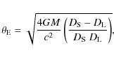
|
(1) |
where
In many cases, the source trajectory happens to cross a caustic. As
the source crosses the caustic curve and enters the enclosed area, a
new pair of images appears, causing a sudden increase in the observed
brightness. In a similar way, when the source exits the area defined by the
caustics, the two images merge and disappear, causing a rapid drop in
the observed brightness. These dramatic changes in
magnification result in readily recognisable jumps in microlensing
light curves. As emphasised by Cassan (2008), the ingress and
egress times
![]() and
and
![]() may be restricted to within very tight
intervals when caustic crossing features have been identified in the
light curve, and thus advantageously used as alternative modelling
parameters.
may be restricted to within very tight
intervals when caustic crossing features have been identified in the
light curve, and thus advantageously used as alternative modelling
parameters.
The new set of binary-lens modelling parameters introduced by
Cassan (2008) have the advantage that two of these
parameters are very closely related
to features that can be directly identified in the light
curve. Using this new formulation to analyse the data of OGLE 2007-BLG-472 in
its most straightforward implementation as a maximum likelihood analysis
(``minimising ![]() ''), Kains et al. (2009) unveiled a subtle
aspect of binary-lens modelling: relatively improbable physical
models with very large values of
''), Kains et al. (2009) unveiled a subtle
aspect of binary-lens modelling: relatively improbable physical
models with very large values of
![]() were found with
were found with ![]() values lower than other more plausible models.
To avoid finding parameter combinations that are physically
unlikely, dramatic progress can be achieved by switching to a Bayesian
analysis. This is desirable as the Bayesian approach makes use of prior
information on the underlying physical parameters, while
values lower than other more plausible models.
To avoid finding parameter combinations that are physically
unlikely, dramatic progress can be achieved by switching to a Bayesian
analysis. This is desirable as the Bayesian approach makes use of prior
information on the underlying physical parameters, while ![]() says
nothing about parameter plausibility.
says
nothing about parameter plausibility.
In this article, we show how to derive Bayesian priors for the
caustic-crossing binary-lens parameters defined by Cassan (2008). These are
based on physical priors on quantities that can be estimated from Galactic
models or calculated from already observed events (Sects. 2 and
3). In Sect. 4, we describe an
implementation of this Bayesian formalism within a Markov chain
Monte Carlo fitting scheme, using in particular priors on the
Einstein time
![]() (time for the source to travel an angular
distance
(time for the source to travel an angular
distance
![]() ).
).
2 Maximum likelihood versus Bayesian fitting
Cassan (2008) introduced a new parameterisation of the binary
lens microlens light curve model that is well suited to
describing caustic-crossing events. In this formalism, the caustic curve in the
source plane is parameterised by a curvilinear abscissa (or arc
length) from 0 to 2. The trajectory of a source
crossing a caustic, which is classically parameterised by its
impact parameter
![]() and position angle
and position angle ![]() ,
can alternatively
be defined by giving the values
,
can alternatively
be defined by giving the values
![]() at ingress and
at ingress and
![]() at
egress
at
egress![]() .
The two parameters timing the trajectory,
.
The two parameters timing the trajectory,
![]() (time to cross
one Einstein radius) and
(time to cross
one Einstein radius) and
![]() (date at minimum impact parameter
(date at minimum impact parameter
![]() ), are then replaced by the ingress and
egress times
), are then replaced by the ingress and
egress times
![]() and
and
![]() .
The caustic curve is specified in
the source (i.e., caustic) plane by a complex function
.
The caustic curve is specified in
the source (i.e., caustic) plane by a complex function
![]() (see Sect. 3.2), and once
(see Sect. 3.2), and once
![]() and
and
![]() are specified,
the source trajectory is fully defined.
This bijective switch of parameters,
are specified,
the source trajectory is fully defined.
This bijective switch of parameters,
![]() ,
takes advantage of the relatively high precision with which
,
takes advantage of the relatively high precision with which
![]() and
and
![]() can be inferred from the observations
(Kubas et al. 2005; Kains et al. 2009).
can be inferred from the observations
(Kubas et al. 2005; Kains et al. 2009).
Using these new parameters, Kains et al. (2009) analysed the caustic
crossing event OGLE 2007-BLG-472. The approach taken was
a maximum likelihood procedure, quantifying the ``goodness-of-fit''
by a ![]() statistic, and
minimising the
statistic, and
minimising the ![]() to optimise the fit.
A grid search in (d,q) with even spacing in
to optimise the fit.
A grid search in (d,q) with even spacing in ![]() and
and ![]() was conducted. For each (d,q) caustic configuration, a genetic
algorithm was used to explore widely the remaining parameter space.
While
was conducted. For each (d,q) caustic configuration, a genetic
algorithm was used to explore widely the remaining parameter space.
While
![]() covered the full range of possibilities,
covered the full range of possibilities,
![]() ,
,
![]() and
and
![]() evolved in very tight
intervals based on the values inferred from the light curve features
(caustic crossing magnification peaks).
These first fits were refined using a Markov chain Monte Carlo (MCMC)
algorithm, again holding (d,q) fixed while optimising the remaining
parameters. The best-fit models in each of the identified best-fit
regions were then found by allowing all parameters to vary.
evolved in very tight
intervals based on the values inferred from the light curve features
(caustic crossing magnification peaks).
These first fits were refined using a Markov chain Monte Carlo (MCMC)
algorithm, again holding (d,q) fixed while optimising the remaining
parameters. The best-fit models in each of the identified best-fit
regions were then found by allowing all parameters to vary.
As expected for binary lens events, the resulting
![]() maps
uncovered a variety of widely-separated model parameter regions
where a relatively low
maps
uncovered a variety of widely-separated model parameter regions
where a relatively low ![]() could be achieved.
The lowest
could be achieved.
The lowest ![]() models corresponded to very low q,
in the planet-mass regime. But with a short duration between the
caustic entry and exit, and a planetary caustic size scaling as
q1/2, these models implied an extremely long Einstein time
models corresponded to very low q,
in the planet-mass regime. But with a short duration between the
caustic entry and exit, and a planetary caustic size scaling as
q1/2, these models implied an extremely long Einstein time
![]() days, which
is very unlikely according to kinematics of stars motions within the
Milky Way. These best-fit maximum likelihood models were therefore
rejected on this physical argument.
This need to reject the lowest
days, which
is very unlikely according to kinematics of stars motions within the
Milky Way. These best-fit maximum likelihood models were therefore
rejected on this physical argument.
This need to reject the lowest ![]() models
highlights a weakness in the maximum likelihood approach,
which neglects prior distributions on the parameter space.
On the other hand, Bayesian parameter estimation takes proper
account of prior distributions in the parameter space
(see e.g., Trotta 2008, for a review of astrophysical applications).
models
highlights a weakness in the maximum likelihood approach,
which neglects prior distributions on the parameter space.
On the other hand, Bayesian parameter estimation takes proper
account of prior distributions in the parameter space
(see e.g., Trotta 2008, for a review of astrophysical applications).
In a Bayesian analysis, the posterior probability distribution over
the model parameters ![]() is a function of the data D
is a function of the data D
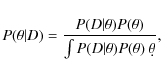
|
(2) |
where
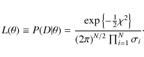
|
(3) |
Since maximising the likelihood corresponds to minimising
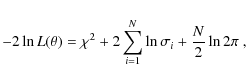
|
(4) |
a maximum likelihood is equivalent to a minimum in
3 A Bayesian prior for (s ,s
,s
 )
)
3.1 Distribution of (s,s
)
for isotropic trajectories
A uniform prior probability distribution in the parameter square
![]() is implicit in the maximum likelihood
analysis. Because of the non-linear correspondence between the two
sets of parameters, it should correspond to a rather unlikely prior
for the
is implicit in the maximum likelihood
analysis. Because of the non-linear correspondence between the two
sets of parameters, it should correspond to a rather unlikely prior
for the
![]() source trajectory parameters.
A more plausible prior would for example arrange for the source
trajectories to be uniformly distributed and isotropic in
orientation.
source trajectory parameters.
A more plausible prior would for example arrange for the source
trajectories to be uniformly distributed and isotropic in
orientation.
In Fig. 1, the top panel shows an intermediate
caustic with d=1.1 and q=0,1 (i.e., six cusps, in orange) with several crossing
trajectories. It can be seen that a straight
line may cross the caustic at two (black line), four (red line), or
six (blue line) locations, depending on the number and orientation
of the cusps. In the bottom panel, ![]() 104 of these trajectories
were randomly shot and their corresponding position in the
104 of these trajectories
were randomly shot and their corresponding position in the
![]() square reported, using the same colour convention.
Trajectories with a single pair of ingress and egress map into
unique black points, while for red and blue trajectory lines, there
are respectively two and three possible pairs of ingress and egress
points.
square reported, using the same colour convention.
Trajectories with a single pair of ingress and egress map into
unique black points, while for red and blue trajectory lines, there
are respectively two and three possible pairs of ingress and egress
points.
![\begin{figure}
\par\hspace*{5mm}\includegraphics[width=7.4cm]{13755fig1a.eps}\\
\includegraphics[width=9cm]{13755fig1b.eps}
\end{figure}](/articles/aa/full_html/2010/07/aa13755-09/img36.png)
|
Figure 1:
The top panel illustrates
the three kinds of possible source trajectories crossing a
caustic: the black line has a single pair of ingress and
egress points, while the red and blue lines have, respectively,
two and three ingress/egress points. The bottom panel shows
in the
|
| Open with DEXTER | |
We can understand some of the structures in the bottom panel of
Fig. 1 as follows:
vertical and horizontal lines marking the s values at the cusps
divide the
![]() square into boxes. No trajectories appear
in the boxes along the diagonal because the caustics curve
concavely outward. It is thus impossible for a line that enters
at some position between two cusps to exit at any point between
those two cusps. In a similar way, other empty regions correspond to
ingress/egress pairs that cannot be realised by straight lines
crossing the caustic.
The trajectories are seen to bunch up
around ingress/egress pairs occurring close to a cusp.
This happens because any trajectory entering close to a cusp is
very likely (for a wide range of angles) to also exit near
the same cusp.
square into boxes. No trajectories appear
in the boxes along the diagonal because the caustics curve
concavely outward. It is thus impossible for a line that enters
at some position between two cusps to exit at any point between
those two cusps. In a similar way, other empty regions correspond to
ingress/egress pairs that cannot be realised by straight lines
crossing the caustic.
The trajectories are seen to bunch up
around ingress/egress pairs occurring close to a cusp.
This happens because any trajectory entering close to a cusp is
very likely (for a wide range of angles) to also exit near
the same cusp.
3.2 Analytical formulation
We develop a mathematical formulation that allows us
to compute analytically priors on
![]() .
The lens
equation for a binary lens with separation d and mass ratio q defines the mapping of the position of a point-source
.
The lens
equation for a binary lens with separation d and mass ratio q defines the mapping of the position of a point-source ![]() on the
source plane to the positions of its three or five images at z on
the lens plane
on the
source plane to the positions of its three or five images at z on
the lens plane
where the more massive body is at the centre and the companion on the left-hand side. Following Witt (1990), the caustic lines
![\begin{displaymath}\frac{1}{1+q}\left[\frac{1}{z^2} +
\frac{q}{(z+d)^2}\right] = {\rm e}^{-{\rm i}\phi} ,
\end{displaymath}](/articles/aa/full_html/2010/07/aa13755-09/img40.png)
where z and
| Figure 2:
Bayesian prior
|
|
| Open with DEXTER | |
To write more condensed formulae, we use notations that
resemble two-dimensional vector operations.
Given two complex numbers
![]() and
and
![]() ,
we write
,
we write
![]() (``wedge
product'') and
(``wedge
product'') and
![]() (``scalar product''), which are both real numbers.
Moreover, a quantity related to a caustic entry (exit)
is indicated by a subscript ``
(``scalar product''), which are both real numbers.
Moreover, a quantity related to a caustic entry (exit)
is indicated by a subscript ``![]() '' (``
'' (``![]() '').
Using the usual convention that
'').
Using the usual convention that
![]() when the origin of the
coordinate system stays on the right-hand side of the source
trajectory, one can write
when the origin of the
coordinate system stays on the right-hand side of the source
trajectory, one can write

![\begin{displaymath}{t_{\rm0}}= \frac{t_{\rm out}+t_{\rm in}}{2} - (t_{\rm out}-t...
...eft\vert\zeta_{\rm out}-\zeta_{\rm in}\right\vert^2}\right],
\end{displaymath}](/articles/aa/full_html/2010/07/aa13755-09/img54.png)
where H is the Heaviside step function, and
|
(11) |
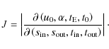
Since the dependencies of the classical parameters with respect to the new ones are
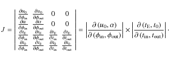
|
(12) |
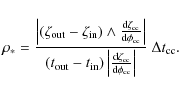
After some algebra, we find for the components of the two latter Jacobians
| |
= | 
|
|
| = | ![$\displaystyle \frac{\left(\zeta_{\rm out}-\zeta_{\rm in}\right)\cdot\zeta_{\rm ...
...m in}\right) \wedge
\frac{{\rm d}\zeta_{\rm in}}{{\rm d}\phi_{\rm in}}\right] ,$](/articles/aa/full_html/2010/07/aa13755-09/img65.png)
|
(13) | |
| = | ![$\displaystyle - \frac{\left(\zeta_{\rm out}-\zeta_{\rm in}\right)\cdot\zeta_{\r...
...in}\right) \wedge
\frac{{\rm d}\zeta_{\rm out}}{{\rm d}\phi_{\rm out}}\right] ,$](/articles/aa/full_html/2010/07/aa13755-09/img67.png)
|
(14) | |
| = | 
|
||
| = | 
|
(15) | |
| = | 
|
(16) | |
| = | (17) | ||
| = | (18) | ||
| = | ![$\displaystyle \frac{1}{2} + \left[\frac{1}{2}\frac{\zeta_{\rm out}+\zeta_{\rm i...
...zeta_{\rm in}}
{\left\vert\zeta_{\rm out}-\zeta_{\rm in}\right\vert^2}\right] ,$](/articles/aa/full_html/2010/07/aa13755-09/img78.png)
|
(19) | |
| = | ![$\displaystyle \frac{1}{2} - \left[\frac{1}{2}\frac{\zeta_{\rm out}+\zeta_{\rm i...
...zeta_{\rm in}}
{\left\vert\zeta_{\rm out}-\zeta_{\rm in}\right\vert^2}\right] ,$](/articles/aa/full_html/2010/07/aa13755-09/img80.png)
|
(20) |
so that


which gives
The derivatives
where
|
(25) |
In the limit of cusp-crossing trajectories, i.e.,
As expected, the Jacobian J is a function of
the two parameters
![]() ,
while the
bijection between the two set of parameters was possible by involving
,
while the
bijection between the two set of parameters was possible by involving
![]() .
However, J is not yet the
Bayesian prior
.
However, J is not yet the
Bayesian prior
![]() we seek. We have
yet to consider two aspects. Firstly, the parameters
we seek. We have
yet to consider two aspects. Firstly, the parameters
![]() are themselves affected by prior
probability distributions; this is discussed at the end of this
section and is the topic of Sect. 4.1.
Secondly, caustic crossing points
are either entries or exits since the trajectory is orientated from
are themselves affected by prior
probability distributions; this is discussed at the end of this
section and is the topic of Sect. 4.1.
Secondly, caustic crossing points
are either entries or exits since the trajectory is orientated from
![]() to
to
![]() (
(
![]() ), which is not
accounted for in Eq. (23).
To solve this second issue, we calculate the outward normal vector to the
caustics at point
), which is not
accounted for in Eq. (23).
To solve this second issue, we calculate the outward normal vector to the
caustics at point ![]() ,
,
as well as the normalised and orientated trajectory vector
and check whether
Defined in this way,
![]() is thus
the prior on
is thus
the prior on
![]() that we seek, in the special case
of isotropic source trajectories (uniform distributions for
that we seek, in the special case
of isotropic source trajectories (uniform distributions for
![]() and
and
![]() ), uniform microlensing events rate (
), uniform microlensing events rate (
![]() is a random
number), and uniform Einstein time
is a random
number), and uniform Einstein time
![]() .
In Fig. 2, we have plotted
.
In Fig. 2, we have plotted
![]() for
various (d,q) configurations as a
function of
for
various (d,q) configurations as a
function of
![]() (horizontal axis) and
(horizontal axis) and
![]() (vertical axis),
higher values of P appearing in white (linear scale).
From left to right, these configurations are: (a) intermediate with
d=1.1 and q=0.1; (b) wide+central and (c) wide+secondary, both
configurations for d=2 and q=0.1; (d) close+central and (e)
close+secondary caustic, both for
d=0.5 and q=0.1. One can compare the intermediate case plot with
Fig. 1. In Sect. 4.1, we investigate how
assuming different priors on the Einstein time
(vertical axis),
higher values of P appearing in white (linear scale).
From left to right, these configurations are: (a) intermediate with
d=1.1 and q=0.1; (b) wide+central and (c) wide+secondary, both
configurations for d=2 and q=0.1; (d) close+central and (e)
close+secondary caustic, both for
d=0.5 and q=0.1. One can compare the intermediate case plot with
Fig. 1. In Sect. 4.1, we investigate how
assuming different priors on the Einstein time
![]() affect the prior
on
affect the prior
on
![]() .
.
3.3 Extended sources
When the source approaches the caustic curves (at typically less than
three projected source radii), one needs to take into account extended
source effects in the modelling. As for
![]() and
and
![]() ,
it is usually possible to extract from the light curve a new
parameter that can be used instead of the source radius.
,
it is usually possible to extract from the light curve a new
parameter that can be used instead of the source radius.
It is well known that when the source crosses a straight
line caustic (which is in many cases a good approximation of a real
caustic), one can easily infer the duration of the crossing
from the shape of the caustic crossing feature itself
(Cassan et al. 2004; Schneider & Wagoner 1987; Albrow et al. 1999). Here, we
define this duration as the time for the source to cross
the caustic line by its full radius (i.e., from centre to limb), so that
![]() .
In this definition,
.
In this definition,
![]() is the source radius in Einstein ring radius units,
is the source radius in Einstein ring radius units,
![]() is the component of the source velocity perpendicular to
the caustic, and the subscript ``cc'' refers to either the caustic
entry (``in'') or exit (``out''). For a given absolute velocity
is the component of the source velocity perpendicular to
the caustic, and the subscript ``cc'' refers to either the caustic
entry (``in'') or exit (``out''). For a given absolute velocity
![]() ,
the source will take longer to cross the caustic if the
trajectory makes a tangential angle with it.
More precisely, the normal velocity is
proportional to the cosine of the angle between the trajectory and
the caustic normal
,
the source will take longer to cross the caustic if the
trajectory makes a tangential angle with it.
More precisely, the normal velocity is
proportional to the cosine of the angle between the trajectory and
the caustic normal
![]() .
Inserting into this equation the expressions for
.
Inserting into this equation the expressions for
![]() ,
,
![]() ,
and
,
and
![]() (Eqs. (9),
(26), and (27), respectively), we can compute the
source radius
(Eqs. (9),
(26), and (27), respectively), we can compute the
source radius
![]() as a function of
as a function of
![]()
This expression would be exact if the crossed caustic were a perfect and infinite straight line. In reality, however, caustic curves always have a curvature, and sometimes the source partly crosses a cusp. Nevertheless, there is no arguing that
4 Markov Chain Monte Carlo fitting
4.1 Examples of prior probability distributions
For a given set of fitting parameters
![]() ,
the prior of the probed model is given by
,
the prior of the probed model is given by
The prior
![\begin{figure}
\par\includegraphics[width=5cm]{13755fig3.eps}
\end{figure}](/articles/aa/full_html/2010/07/aa13755-09/img116.png)
|
Figure 3:
Prior
|
| Open with DEXTER | |
The first class of priors that we can use are uninformative priors. Since
the prior expresses information about the values of parameters before
any data has been taken, we know that parameters such as
![]() ,
,
![]() ,
or
,
or
![]() must have uninformative priors,
because we can only estimate their values by examining the light curve.
Although it is natural to use uniform priors for
must have uninformative priors,
because we can only estimate their values by examining the light curve.
Although it is natural to use uniform priors for
![]() ,
,
![]() or
or
![]() ,
for strictly positive parameters such as
,
for strictly positive parameters such as
![]() or
or
![]() ,
it is more suitable and commonly decided to
use an uninformative prior that is uniform in the logarithm of the parameter.
,
it is more suitable and commonly decided to
use an uninformative prior that is uniform in the logarithm of the parameter.
We illustrate the use of an uninformative prior (uniform priors in
![]() ,
in
,
in
![]() ,
,
![]() ,
and
,
and
![]() )
by computing
)
by computing
![]() for the solution configuration
of the binary lens event OGLE 2002-BLG-069
(Kubas et al. 2005; Cassan et al. 2004).
The configuration for that event was that of a source
crossing the central caustic of a close binary lens with parameters
d=0.46, q=0.58 and
for the solution configuration
of the binary lens event OGLE 2002-BLG-069
(Kubas et al. 2005; Cassan et al. 2004).
The configuration for that event was that of a source
crossing the central caustic of a close binary lens with parameters
d=0.46, q=0.58 and
![]() days.
The resulting prior
days.
The resulting prior
![]() is
plotted in Fig. 3, where the red cross shows the location of the caustic
crossings at
is
plotted in Fig. 3, where the red cross shows the location of the caustic
crossings at
![]() ,
,
![]() .
This falls
within a region of high probability, meaning that the corresponding
.
This falls
within a region of high probability, meaning that the corresponding
![]() prior would have been a
reasonable choice for this event.
prior would have been a
reasonable choice for this event.
The second class of priors are those that we can derive using
information known before the event is observed. In microlensing,
a convenient parameter on which such a prior can be placed is the
Einstein time
![]() .
This parameter depends on the
relative distances between the source, the lens, and the observer, the
kinematics of both the lens and the source and the lens' mass
function. Combining all these data can help us to determine
which ranges of values of
.
This parameter depends on the
relative distances between the source, the lens, and the observer, the
kinematics of both the lens and the source and the lens' mass
function. Combining all these data can help us to determine
which ranges of values of
![]() are more likely to be
observed. For the event OGLE-2007-BLG-472 (Kains et al. 2009), no prior
information was included on
are more likely to be
observed. For the event OGLE-2007-BLG-472 (Kains et al. 2009), no prior
information was included on
![]() (or the prior was assumed
to be uninformative), which cause the best-fit models to have
unrealistically long
(or the prior was assumed
to be uninformative), which cause the best-fit models to have
unrealistically long
![]() .
.
The method presented here can
indeed be extended to include informative priors on parameters
other than
![]() ,
such as the source flux distribution, the
blending light due to the lens, the relative proper motion of the
source and lens, or the source-radius caustic crossing-time, but this
would require us to link the analysis to a Monte Carlo model of the
Galaxy. Although our approach can be generalised to these possible
extensions, they are beyond the scope of the present
paper. Using
,
such as the source flux distribution, the
blending light due to the lens, the relative proper motion of the
source and lens, or the source-radius caustic crossing-time, but this
would require us to link the analysis to a Monte Carlo model of the
Galaxy. Although our approach can be generalised to these possible
extensions, they are beyond the scope of the present
paper. Using
![]() also has the advantage that its statistical
distribution is fairly well-constrained by observed single-lens light
curves, since this parameter is common to single- and binary-lens
events.
also has the advantage that its statistical
distribution is fairly well-constrained by observed single-lens light
curves, since this parameter is common to single- and binary-lens
events.
![\begin{figure}
\par\includegraphics[width=9cm, bb= 33 0 760 443]{13755fig4a.eps}...
...e*{2cm}\includegraphics[width=5cm]{13755fig4b.eps}\hspace*{2cm}}
\end{figure}](/articles/aa/full_html/2010/07/aa13755-09/img120.png)
|
Figure 4:
In the top panel, the histogram (blue rectangles) shows the
distribution of
|
| Open with DEXTER | |
Empirical distributions of
![]() can be obtained by
modelling a large number of observed microlensing events. The top
panel of Fig. 4 shows a histogram (blue rectangles) of
can be obtained by
modelling a large number of observed microlensing events. The top
panel of Fig. 4 shows a histogram (blue rectangles) of
![]() values found by fitting 788 single-lens microlensing
events from the 2006-2007 OGLE seasons (including blending). As
expected, the distribution is far from uniform but instead appears
roughly log-normal with a peak close to
values found by fitting 788 single-lens microlensing
events from the 2006-2007 OGLE seasons (including blending). As
expected, the distribution is far from uniform but instead appears
roughly log-normal with a peak close to
![]() and
and
![]() .
Theoretical
distributions of
.
Theoretical
distributions of
![]() can also be based on predictions
obtained with a Galactic model, such as the distribution
advocated by Wood & Mao (2005). This is plotted as a solid black
line on top of our histogram (Fig. 4, top panel) and is seen
to closely match the empirical distribution.
Nevertheless, the distribution of Wood & Mao (2005) lacks both
extremely long events (say
can also be based on predictions
obtained with a Galactic model, such as the distribution
advocated by Wood & Mao (2005). This is plotted as a solid black
line on top of our histogram (Fig. 4, top panel) and is seen
to closely match the empirical distribution.
Nevertheless, the distribution of Wood & Mao (2005) lacks both
extremely long events (say
![]() days) that can be interpreted
as black hole lenses, and extremely short events
(say
days) that can be interpreted
as black hole lenses, and extremely short events
(say
![]() days) that can be interpreted as
evidence of a population of free floating planets. But selection effects
cause these extreme events to be under-represented in the observed
days) that can be interpreted as
evidence of a population of free floating planets. But selection effects
cause these extreme events to be under-represented in the observed
![]() distribution, as can be seen in Fig. 4. For these exceptional cases,
special treatment would be required, for example using a prior on
distribution, as can be seen in Fig. 4. For these exceptional cases,
special treatment would be required, for example using a prior on
![]() that is more generous to extreme values in an attempt to compensate
for selection effects. For most of binary lens events, however, a mild
discrimination against black hole or loose planet lenses seems
appropriate.
that is more generous to extreme values in an attempt to compensate
for selection effects. For most of binary lens events, however, a mild
discrimination against black hole or loose planet lenses seems
appropriate.
Using the Wood & Mao (2005) distribution as a prior, we compute and
plot (Fig. 4, bottom panel) the corresponding distribution
![]() by assuming
by assuming
![]() days, d=1.1, and
q=0.1 (the same intermediate configuration as Fig. 2).
Figure 4 (bottom panel) shows that with this prior,
cusp-crossing trajectories are far less
likely to happen. For a trajectory near the cusps, this is because
the source has only a short distance to travel between the entry
and exit, while
days, d=1.1, and
q=0.1 (the same intermediate configuration as Fig. 2).
Figure 4 (bottom panel) shows that with this prior,
cusp-crossing trajectories are far less
likely to happen. For a trajectory near the cusps, this is because
the source has only a short distance to travel between the entry
and exit, while
![]() is constant, meaning that the
source's motion has to be very slow, leading to large
values of
is constant, meaning that the
source's motion has to be very slow, leading to large
values of
![]() ,
which are now ruled out
by the prior
,
which are now ruled out
by the prior![]() .
This effect can be seen directly in the plot of
.
This effect can be seen directly in the plot of
![]() ,
where strong ``wing'' features at the cusps
disappear, and other features appear (compare with Fig. 2).
,
where strong ``wing'' features at the cusps
disappear, and other features appear (compare with Fig. 2).
4.2 Posterior probability distributions: MCMC fitting
In practice, these and other statistics related to the posterior
parameter distribution can be
evaluated efficiently using a Markov chain Monte Carlo
to evaluate the probability-weighted integrals in Bayes' theorem.
A random walk in the parameter space is undertaken by
taking random steps drawn from a distribution of the parameters ![]() .
Each proposed step is accepted or rejected based on
the probability of the new point relative to the old one exceeding
some threshold, which is adjusted to maintain the acceptance rate
above roughly 20-30%.
The resulting chain locates and wanders around a local minimum,
sampling the parameters with a weight proportional to
the posterior probability.
.
Each proposed step is accepted or rejected based on
the probability of the new point relative to the old one exceeding
some threshold, which is adjusted to maintain the acceptance rate
above roughly 20-30%.
The resulting chain locates and wanders around a local minimum,
sampling the parameters with a weight proportional to
the posterior probability.
For a maximum likelihood analysis, the relative probability
used to accept or reject new steps is
![]() alone, where
alone, where
![]() is the
is the ![]() difference between the new and old
points; in a full Bayesian analysis, we multiply this exponential factor by the
ratio of new to old values of the prior
difference between the new and old
points; in a full Bayesian analysis, we multiply this exponential factor by the
ratio of new to old values of the prior
![]() ,
following
Eq. (29).
The posterior probability that the parameters
,
following
Eq. (29).
The posterior probability that the parameters ![]() lie in a defined
region
lie in a defined
region ![]() is then
is then
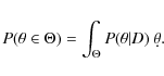
|
(30) |
The expected value of any function of parameters,
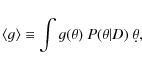
|
(31) |
and the variance about that expected value is
![\begin{displaymath}{\rm Var} \left[ g(\theta) \right] \equiv \int
\left( g(\th...
... - \left< g \right> \right)^2~
P(\theta\vert D)~ \d \theta .
\end{displaymath}](/articles/aa/full_html/2010/07/aa13755-09/img138.png)
|
(32) |
In a similar way, confidence intervals, parameter covariances, and confidence intervals can all be evaluated easily in the usual manner given the posterior probability distribution found with the MCMC algorithm, providing us with a complete statistical picture of the parameter space that we explore.
5 Conclusion
We have investigated plausible priors for Bayesian analysis of caustic-crossing microlensing light curves, based on an alternative parameterisation introduced by Cassan (2008). We have developed a mathematical formulation that allows us to compute analytically Bayesian priors for these parameters, given the knowledge we have about the physical quantities on which they depend. A number of relevant priors that may be used in a Bayesian, Markov chain Monte Carlo implementation of the given equations have been explored.
In the context of the rapid development of a new generation of networks of classical and robotic telescopes (e.g., Tsapras et al. 2009), as well as space-based observations such as with the ESA project satellite Euclid (Beaulieu et al. 2010), a current challenge facing the microlens planet search community is to fully automate the fitting of binary lens light curves in real time, after having detected an anomaly (e.g., Horne et al. 2009). This would enable anomalies that are detected in the observed light curves to be characterised as quickly as possible and for us to ascertain whether the anomalous behaviour is caused by a planet-mass companion of the lens star. Identifying parameters that could be estimated automatically by analysing the light curve (e.g., a magnification jump due to a caustic crossing) is already a step forward in accelerating the fitting codes by exploring a far more tighter parameter space. This was the motivation of Cassan (2008) in defining a new set of parameters. In this work, we have added the possibility of including Bayesian priors in the analysis, which would avoid the need to explore combinations of parameters that are unlikely to happen.
References
- Albrow, M. D., Beaulieu, J.-P., Caldwell, J. A. R., et al. 1999, ApJ, 522, 1022 [NASA ADS] [CrossRef] [Google Scholar]
- Beaulieu, J. P., Bennett, D. P., Batista, V., et al. 2010, unpublished[arXiv:1001.3349] [Google Scholar]
- Beaulieu, J.-P., Bennett, D. P., Fouqué, P., et al. 2006, Nature, 439, 437 [NASA ADS] [CrossRef] [PubMed] [Google Scholar]
- Bond, I. A., Abe, F., Dodd, R. J., et al. 2001, MNRAS, 327, 868 [NASA ADS] [CrossRef] [Google Scholar]
- Cassan, A. 2008, A&A, 491, 587 [NASA ADS] [CrossRef] [EDP Sciences] [Google Scholar]
- Cassan, A., Beaulieu, J. P., Brillant, S., et al. 2004, A&A, 419, L1 [NASA ADS] [CrossRef] [EDP Sciences] [Google Scholar]
- Einstein, A. 1936, Science, 84, 506 [NASA ADS] [CrossRef] [PubMed] [Google Scholar]
- Gould, A., & Loeb, A. 1992, ApJ, 396, 104 [NASA ADS] [CrossRef] [Google Scholar]
- Horne, K., Snodgrass, C., & Tsapras, Y. 2009, MNRAS, 396, 2087 [NASA ADS] [CrossRef] [Google Scholar]
- Kains, N., Cassan, A., Horne, K., et al. 2009, MNRAS, 395, 787 [NASA ADS] [CrossRef] [Google Scholar]
- Kubas, D., Cassan, A., Beaulieu, J. P., et al. 2005, A&A, 435, 941 [NASA ADS] [CrossRef] [EDP Sciences] [Google Scholar]
- Kubas, D., Cassan, A., Dominik, M., et al. 2008, A&A, 483, 317 [NASA ADS] [CrossRef] [EDP Sciences] [Google Scholar]
- Mao, S., & Paczynski, B. 1991, ApJ, 374, L37 [NASA ADS] [CrossRef] [Google Scholar]
- Paczynski, B. 1986, ApJ, 304, 1 [NASA ADS] [CrossRef] [Google Scholar]
- Schneider, P., & Wagoner, R. V. 1987, ApJ, 314, 154 [NASA ADS] [CrossRef] [Google Scholar]
- Trotta, R. 2008, Contemporary Physics, 49, 71 [NASA ADS] [CrossRef] [Google Scholar]
- Tsapras, Y., Street, R., Horne, K., et al. 2009, AN, 330, 4 [Google Scholar]
- Udalski, A. 2003, Acta Astron., 53, 291 [NASA ADS] [Google Scholar]
- Witt, H. J. 1990, A&A, 236, 311 [NASA ADS] [Google Scholar]
- Wood, A., & Mao, S. 2005, MNRAS, 362, 945 [NASA ADS] [CrossRef] [Google Scholar]
Footnotes
- ... OGLE
![[*]](/icons/foot_motif.png)
- http://www.astrouw.edu.pl/ ogle
- ... MOA
- http://www.phys.canterbury.ac.nz/moa
- ... PLANET
- http://planet.iap.fr
- ...
 FUN
FUN
- http://www.astronomy.ohio-state.edu/ microfun
- ... RoboNet
- http://robonet.lcogt.net
- ... MiNDSTEp
- http://www.mindstep-science.org
- ... egress
- We use the notations ``in'' and ``out'' in place of ``entry'' and ``exit'' of Cassan (2008) to write more condensed formulae.
- ... prior
- More precisely, when
 ,
Wood & Mao (2005)
,
Wood & Mao (2005)
 distribution
behaves like
distribution
behaves like 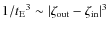 ,
and since
,
and since  ,
the net result is that near cusps,
,
the net result is that near cusps,  .
.
All Figures
|
|
Figure 1:
The top panel illustrates
the three kinds of possible source trajectories crossing a
caustic: the black line has a single pair of ingress and
egress points, while the red and blue lines have, respectively,
two and three ingress/egress points. The bottom panel shows
in the
|
| Open with DEXTER | |
| In the text | |
| |
Figure 2:
Bayesian prior
|
| Open with DEXTER | |
| In the text | |
|
|
Figure 3:
Prior
|
| Open with DEXTER | |
| In the text | |
|
|
Figure 4:
In the top panel, the histogram (blue rectangles) shows the
distribution of
|
| Open with DEXTER | |
| In the text | |
Copyright ESO 2010
Current usage metrics show cumulative count of Article Views (full-text article views including HTML views, PDF and ePub downloads, according to the available data) and Abstracts Views on Vision4Press platform.
Data correspond to usage on the plateform after 2015. The current usage metrics is available 48-96 hours after online publication and is updated daily on week days.
Initial download of the metrics may take a while.