| Issue |
A&A
Volume 515, June 2010
|
|
|---|---|---|
| Article Number | A16 | |
| Number of page(s) | 18 | |
| Section | Catalogs and data | |
| DOI | https://doi.org/10.1051/0004-6361/200913236 | |
| Published online | 02 June 2010 | |
Photometric multi-site campaign on the open cluster NGC 884
I. Detection of the variable stars![[*]](/icons/foot_motif.png)
S. Saesen1,![]() - F. Carrier1,
- F. Carrier1,![]() - A. Pigulski2
- C. Aerts1,3 - G. Handler4
- A. Narwid2 -
J. N. Fu5 - C. Zhang5
- X. J. Jiang6 -
J. Vanautgaerden1 - G. Kopacki2
- M. Steslicki2 - B. Acke1,
- A. Pigulski2
- C. Aerts1,3 - G. Handler4
- A. Narwid2 -
J. N. Fu5 - C. Zhang5
- X. J. Jiang6 -
J. Vanautgaerden1 - G. Kopacki2
- M. Steslicki2 - B. Acke1,![]() - E. Poretti7 - K. Uytterhoeven7,8
- C. Gielen1 - R. Østensen1
- W. De Meester1 -
M. D. Reed9 - Z. Ko
- E. Poretti7 - K. Uytterhoeven7,8
- C. Gielen1 - R. Østensen1
- W. De Meester1 -
M. D. Reed9 - Z. Ko![]() aczkowski2
- G. Michalska2 - E. Schmidt4
- K. Yakut1,10,11 - A. Leitner4
- B. Kalomeni12 - M. Cherix13
- M. Spano13 - S. Prins1
- V. Van Helshoecht1 -
W. Zima1 - R. Huygen1
- B. Vandenbussche1 - P. Lenz4,14
- D. Ladjal1 -
E. Puga Antolín1 -
T. Verhoelst1,
aczkowski2
- G. Michalska2 - E. Schmidt4
- K. Yakut1,10,11 - A. Leitner4
- B. Kalomeni12 - M. Cherix13
- M. Spano13 - S. Prins1
- V. Van Helshoecht1 -
W. Zima1 - R. Huygen1
- B. Vandenbussche1 - P. Lenz4,14
- D. Ladjal1 -
E. Puga Antolín1 -
T. Verhoelst1,![]() - J. De Ridder1 -
P. Niarchos15 - A. Liakos15
- D. Lorenz4 - S. Dehaes1
- M. Reyniers1 - G. Davignon1
- S.-L. Kim16 -
D. H. Kim16 -
Y.-J. Lee16 - C.-U. Lee16
- J.-H. Kwon16 - E. Broeders1
- H. Van Winckel1 -
E. Vanhollebeke1 - C. Waelkens1
- G. Raskin1 - Y. Blom1
- J. R. Eggen9 -
P. Degroote1 - P. Beck4
- J. Puschnig4 -
L. Schmitzberger4 -
G. A. Gelven9 -
B. Steininger4 - J. Blommaert1
- R. Drummond1 - M. Briquet1,
- J. De Ridder1 -
P. Niarchos15 - A. Liakos15
- D. Lorenz4 - S. Dehaes1
- M. Reyniers1 - G. Davignon1
- S.-L. Kim16 -
D. H. Kim16 -
Y.-J. Lee16 - C.-U. Lee16
- J.-H. Kwon16 - E. Broeders1
- H. Van Winckel1 -
E. Vanhollebeke1 - C. Waelkens1
- G. Raskin1 - Y. Blom1
- J. R. Eggen9 -
P. Degroote1 - P. Beck4
- J. Puschnig4 -
L. Schmitzberger4 -
G. A. Gelven9 -
B. Steininger4 - J. Blommaert1
- R. Drummond1 - M. Briquet1,![]() - J. Debosscher1
- J. Debosscher1
1 - Instituut voor Sterrenkunde, Katholieke Universiteit Leuven,
Celestijnenlaan 200 D, 3001 Leuven, Belgium
2 - Instytut Astronomiczny Uniwersytetu Wroc![]() awskiego, Kopernika 11, 51-622 Wroc
awskiego, Kopernika 11, 51-622 Wroc![]() aw, Poland
aw, Poland
3 - Department of Astrophysics, Radboud University Nijmegen, PO Box
9010, 6500 GL Nijmegen, The Netherlands
4 - Institut für Astronomie, Universität Wien, Türkenschanzstrasse 17,
1180 Wien, Austria
5 - Department of Astronomy, Beijing Normal University, Beijing 100875,
PR China
6 - National Astronomical Observatories, Chinese Academy of Sciences,
Beijing 100012, PR China
7 - INAF - Osservatorio Astronomico di Brera, via Bianchi 46, 23807
Merate, Italy
8 - Laboratoire AIM, CEA/DSM-CNRS-Université Paris Diderot, CEA,
IRFU, SAp, Centre de Saclay, 91191 Gif-sur-Yvette, France
9
- Department of Physics, Astronomy, & Materials Science,
Missouri
State University, 901 S. National, Springfield, MO 65897, USA
10 - Institute of Astronomy, University of Cambridge, Madingley Road,
Cambridge CB3 0HA, UK
11 - Department of Astronomy & Space Sciences, Ege University,
35100 Izmir, Turkey
12 - Izmir Institute of Technology, Department of Physics, 35430 Izmir,
Turkey
13 - Observatoire de Genève, Université de Genève, Chemin des
Maillettes 51, 1290 Sauverny, Switzerland
14 - Copernicus Astronomical Centre, Bartycka 18, 00-716 Warsaw, Poland
15
- Department of Astrophysics, Astronomy and Mechanics, National and
Kapodistrian University of Athens, Panepistimiopolis, 157 84 Zografos,
Athens, Greece
16 - Korea Astronomy and Space Science Institute, Daejeon 305-348,
South Korea
Received 3 September 2009 / Accepted 9 December 2009
Abstract
Context. Recent progress in the seismic
interpretation of field ![]() Cep
stars has resulted in improvements of the physics in the stellar
structure and evolution models of massive stars. Further asteroseismic
constraints can be obtained from studying ensembles of stars in a young
open cluster, which all have similar age, distance and chemical
composition.
Cep
stars has resulted in improvements of the physics in the stellar
structure and evolution models of massive stars. Further asteroseismic
constraints can be obtained from studying ensembles of stars in a young
open cluster, which all have similar age, distance and chemical
composition.
Aims. To improve our comprehension of the ![]() Cep
stars, we studied the young open cluster NGC 884 to discover
new B-type pulsators, besides the two known
Cep
stars, we studied the young open cluster NGC 884 to discover
new B-type pulsators, besides the two known ![]() Cep stars, and other
variable stars.
Cep stars, and other
variable stars.
Methods. An extensive multi-site campaign was set up
to gather accurate CCD photometry time series in four
filters (U, B, V,
I)
of a field of NGC 884. Fifteen different instruments collected
almost 77 500 CCD images in 1286 h. The
images were
calibrated and reduced to transform the CCD frames into
interpretable differential light curves. Various variability indicators
and frequency analyses were applied to detect variable stars in the
field. Absolute photometry was taken to deduce some general cluster and
stellar properties.
Results. We achieved an accuracy for the brightest
stars of 5.7 mmag in V, 6.9 mmag
in B, 5.0 mmag in I
and 5.3 mmag in U. The noise level
in the amplitude spectra is 50 ![]() mag in the V band.
Our campaign confirms the previously known pulsators, and we report
more than one hundred new multi- and mono-periodic B-, A- and F-type
stars. Their interpretation in terms of classical instability domains
is not straightforward, pointing to imperfections in theoretical
instability computations. In addition, we have discovered six new
eclipsing binaries and four candidates as well as other irregular
variable stars in the observed field.
mag in the V band.
Our campaign confirms the previously known pulsators, and we report
more than one hundred new multi- and mono-periodic B-, A- and F-type
stars. Their interpretation in terms of classical instability domains
is not straightforward, pointing to imperfections in theoretical
instability computations. In addition, we have discovered six new
eclipsing binaries and four candidates as well as other irregular
variable stars in the observed field.
Key words: open clusters and associations: individual: NGC 884 - techniques: photometric - stars: variables: general - stars: oscillations - binaries: eclipsing
1 Introduction
The ![]() Cep
stars are a homogeneous group of B0-B3 stars whose pulsational
behaviour is interpreted in terms of the
Cep
stars are a homogeneous group of B0-B3 stars whose pulsational
behaviour is interpreted in terms of the ![]() mechanism activated
by the metal opacity bump. Given that mainly low-degree low-order
pressure (p-) and gravity (g-)
modes are excited, these stars are good potential targets for in-depth
seismic studies of the interior structure of massive stars.
mechanism activated
by the metal opacity bump. Given that mainly low-degree low-order
pressure (p-) and gravity (g-)
modes are excited, these stars are good potential targets for in-depth
seismic studies of the interior structure of massive stars.
The best-studied ![]() Cep
stars are V836 Cen (Aerts
et al. 2003),
Cep
stars are V836 Cen (Aerts
et al. 2003), ![]() Eridani (Pamyatnykh et al. 2004; Dziembowski
& Pamyatnykh 2008; Ausseloos et al. 2004,
and references given in these papers),
Eridani (Pamyatnykh et al. 2004; Dziembowski
& Pamyatnykh 2008; Ausseloos et al. 2004,
and references given in these papers), ![]() Ophiuchi (Handler
et al. 2005; Briquet et al. 2007,2005),
12 Lacertae (Desmet
et al. 2009; Dziembowski & Pamyatnykh 2008;
Handler
et al. 2006),
Ophiuchi (Handler
et al. 2005; Briquet et al. 2007,2005),
12 Lacertae (Desmet
et al. 2009; Dziembowski & Pamyatnykh 2008;
Handler
et al. 2006), ![]() Canis Majoris (Mazumdar et al. 2006) and
Canis Majoris (Mazumdar et al. 2006) and
![]() Peg
(Handler et al. 2009).
The detailed seismic analysis of these selected stars led to several
new insights into their internal physics. Non-rigid rotation and core
convective overshoot are needed to explain the observed pulsation
frequencies. Moreover, for some of the observed modes of
Peg
(Handler et al. 2009).
The detailed seismic analysis of these selected stars led to several
new insights into their internal physics. Non-rigid rotation and core
convective overshoot are needed to explain the observed pulsation
frequencies. Moreover, for some of the observed modes of ![]() Eridani
and 12 Lacertae excitation problems were encountered (Daszynska-Daszkiewicz et al. 2005).
Eridani
and 12 Lacertae excitation problems were encountered (Daszynska-Daszkiewicz et al. 2005).
The next challenging step in the asteroseismology of ![]() Cep
stars is to measure those stars with much higher signal-to-noise from
space (e.g., Degroote
et al. 2009b)
and to study them in
clusters. Obviously, we would greatly benefit from the fact that the
cluster members have a common origin and formation, implying much
tighter constraints when modelling their observed pulsation behaviour.
Furthermore, clusters are ideally suited for gathering
CCD photometry, providing high-accuracy measurements for
thousands
of stars simultaneously.
Cep
stars is to measure those stars with much higher signal-to-noise from
space (e.g., Degroote
et al. 2009b)
and to study them in
clusters. Obviously, we would greatly benefit from the fact that the
cluster members have a common origin and formation, implying much
tighter constraints when modelling their observed pulsation behaviour.
Furthermore, clusters are ideally suited for gathering
CCD photometry, providing high-accuracy measurements for
thousands
of stars simultaneously.
Three clusters were initially selected for this purpose:
one southern cluster, NGC 3293, which contains eleven
known ![]() Cep
stars (Balona 1994), and
two northern clusters, NGC 6910 and NGC 884, which
contain four and two bona fide
Cep
stars (Balona 1994), and
two northern clusters, NGC 6910 and NGC 884, which
contain four and two bona fide ![]() Cep stars,
respectively (Koaczkowski
et al. 2004; Krzesinski & Pigulski 1997).
Preliminary results for these multi-site cluster campaigns can be found
in Handler
et al. (2007,2008) for NGC 3293, in Pigulski et al. (2007)
and Pigulski (2008) for
NGC 6910 and in Pigulski
et al. (2007) and Saesen et al. (2009,2008)
for NGC 884. In these preliminary reports, the discovery of
some new
Cep stars,
respectively (Koaczkowski
et al. 2004; Krzesinski & Pigulski 1997).
Preliminary results for these multi-site cluster campaigns can be found
in Handler
et al. (2007,2008) for NGC 3293, in Pigulski et al. (2007)
and Pigulski (2008) for
NGC 6910 and in Pigulski
et al. (2007) and Saesen et al. (2009,2008)
for NGC 884. In these preliminary reports, the discovery of
some new ![]() Cep
and other variable stars was already announced.
Cep
and other variable stars was already announced.
This paper deals with the detailed analysis of NGC 884 and is the first in a series on this subject, presenting our data set and discussing the general variability in this cluster.
2 The target cluster NGC 884
NGC 884 (![]() Persei,
Persei,
![]() ,
,
![]() )
is a rich young open cluster located in the Perseus constellation.
Together with NGC 869 (h Persei) it forms the Perseus
double
cluster, which is well documented in the literature.
)
is a rich young open cluster located in the Perseus constellation.
Together with NGC 869 (h Persei) it forms the Perseus
double
cluster, which is well documented in the literature.
The possible co-evolution of both clusters puzzled many
researchers. Some claim that h and ![]() Persei have the same distance modulus
and age, others state that h Persei is closer and younger than
Persei have the same distance modulus
and age, others state that h Persei is closer and younger than
![]() Persei.
For an extensive overview of the photographic, photo-electric and
photometric studies on the co-evolution of the two clusters based on
the age, reddening and distance
moduli, we refer to Southworth
et al. (2004a). They conclude that the most recent
studies (Keller
et al. 2001; Slesnick et al. 2002; Marco &
Bernabeu 2001; Capilla & Fabregat 2002)
converge towards an identical distance modulus of 11.7
Persei.
For an extensive overview of the photographic, photo-electric and
photometric studies on the co-evolution of the two clusters based on
the age, reddening and distance
moduli, we refer to Southworth
et al. (2004a). They conclude that the most recent
studies (Keller
et al. 2001; Slesnick et al. 2002; Marco &
Bernabeu 2001; Capilla & Fabregat 2002)
converge towards an identical distance modulus of 11.7 ![]() 0.05 mag and a log (age/yr) of 7.10
0.05 mag and a log (age/yr) of 7.10 ![]() 0.01 dex. The average reddening of
0.01 dex. The average reddening of ![]() Persei amounts to
E(B-V)=0.56
Persei amounts to
E(B-V)=0.56 ![]() 0.05.
0.05.
Slettebak (1968)
collected rotational
velocities for luminous B giant stars located in the vicinity
of
the double cluster. He reports that the measured stellar rotation
velocities are about 50% higher than for field counterparts,
supported by his observation of an unusual high number of
Be stars in the clusters. More recent projected rotational
velocity measurements of Strom
et al. (2005) confirm that the B stars
in h and ![]() Persei
rotate on average faster than field stars of similar mass and age. More
searches for and studies of Be stars in the clusters have been
carried out, leading to the detection of 20 Be stars
in
Persei
rotate on average faster than field stars of similar mass and age. More
searches for and studies of Be stars in the clusters have been
carried out, leading to the detection of 20 Be stars
in ![]() Persei
(see Malchenko & Tarasov 2008,
and references therein).
Persei
(see Malchenko & Tarasov 2008,
and references therein).
The first variability search in the cluster NGC 884
was conducted by Percy (1972)
in the extreme nucleus of the cluster by means of photo-electric
measurements. He identified three candidate variable stars on a time
scale longer than ten hours, Oo 2088, Oo 2227 and
Oo 2262 (Oosterhoff numbers, see Oosterhoff
1937), and one on a shorter time scale of six hours,
Oo 2299. Waelkens
et al. (1990)
set up a photometric campaign spanning eight years. They report that at
least half of the brighter stars are variable and that most of them
seem to be Be stars. The time sampling of both data sets was
not
suitable to search for ![]() Cep
stars. The campaign
and analysis by Krzesinski &
Pigulski (1997)
yielded more detailed results. Based on a photometric
CCD search
in the central region of NGC 884, they discovered two
Cep
stars. The campaign
and analysis by Krzesinski &
Pigulski (1997)
yielded more detailed results. Based on a photometric
CCD search
in the central region of NGC 884, they discovered two ![]() Cep
stars, Oo 2246 and Oo 2299, showing two and one
pulsation
frequencies, respectively. Furthermore, nine other variables were
found: two eclipsing binaries (Oo 2301,
Oo 2311), three
Be stars (Oo 2088, Oo 2165,
Oo 2242), two
supergiants (Oo 2227, Oo 2417), possibly one
ellipsoidal
binary (Oo 2371), and one variable star of unknown nature
(Oo 2140). Afterwards, a larger cluster field was studied by Krzesinski (1998) and
Krzesinski & Pigulski (2000),
each of them leading to one more
Cep
stars, Oo 2246 and Oo 2299, showing two and one
pulsation
frequencies, respectively. Furthermore, nine other variables were
found: two eclipsing binaries (Oo 2301,
Oo 2311), three
Be stars (Oo 2088, Oo 2165,
Oo 2242), two
supergiants (Oo 2227, Oo 2417), possibly one
ellipsoidal
binary (Oo 2371), and one variable star of unknown nature
(Oo 2140). Afterwards, a larger cluster field was studied by Krzesinski (1998) and
Krzesinski & Pigulski (2000),
each of them leading to one more ![]() Cep candidate:
Oo 2444 and Oo 2809, but the data sets were
insufficient to
confirm their pulsational character. Finally, two papers prior to our
study are devoted to binaries: Southworth
et al. (2004b) investigated the eclipsing binary
Oo 2311 in detail and Malchenko
(2007)
the ellipsoidal variable Oo 2371. Given the
occurrence of
several variables as well as at least one eclipsing binary, we judged
Cep candidate:
Oo 2444 and Oo 2809, but the data sets were
insufficient to
confirm their pulsational character. Finally, two papers prior to our
study are devoted to binaries: Southworth
et al. (2004b) investigated the eclipsing binary
Oo 2311 in detail and Malchenko
(2007)
the ellipsoidal variable Oo 2371. Given the
occurrence of
several variables as well as at least one eclipsing binary, we judged ![]() Persei
to be well suited for our asteroseismology project.
Persei
to be well suited for our asteroseismology project.
3 Equipment and observations
In 2005, a multi-site campaign was set up to gather differential
time-resolved multi-colour CCD photometry of a field of the
cluster NGC 884 that contains the two previously known ![]() Cep
stars. The goal was to collect accurate measurements with a long time
base to make the detection of pulsation frequencies at milli-magnitude
level possible for a large number of cluster stars of the spectral
type B. The observations were taken in different filters to be
able to identify their modes.
Cep
stars. The goal was to collect accurate measurements with a long time
base to make the detection of pulsation frequencies at milli-magnitude
level possible for a large number of cluster stars of the spectral
type B. The observations were taken in different filters to be
able to identify their modes.
The entire campaign spanned 800 days spread over
three
observation seasons. During the first season
(August 2005-March 2006), four telescopes assembled
250 h of data. The main campaign took place in the second
season
(July 2006-March 2007), when nine more telescopes
joined the
project and gathered 940 h of measurements. In the third
season
(July 2007-October 2007), only the two dedicated
telescopes,
the 120-cm Mercator telescope at Observatorio del Roque de los
Muchachos (ORM) and the 60-cm at Bia![]() ków
Observatory, observed NGC 884 for 100 more hours.
In total, an international team consisting of
61 observers used 15 different instruments attached
to
13 telescopes to collect almost
77 500 CCD images
in the UBVI filters and 92 h of
photo-electric data in the ubvy and
UB1BB2V1VG filters.
ków
Observatory, observed NGC 884 for 100 more hours.
In total, an international team consisting of
61 observers used 15 different instruments attached
to
13 telescopes to collect almost
77 500 CCD images
in the UBVI filters and 92 h of
photo-electric data in the ubvy and
UB1BB2V1VG filters.
In Table 1,
an
overview of the different observing sites with their equipment
(telescope, instrument characteristics and filters) is given. Almost
all sites used CCD cameras, only Observatorio Astronómico
Nacional
de San Pedro Mártir (OAN-SPM) and ORM made use of photometers.
Simultaneous Strömgren ![]() and Geneva UB1BB2V1VG measurements
of (suspected)
and Geneva UB1BB2V1VG measurements
of (suspected) ![]() Cep
stars were collected using the Danish photometer at OAN-SPM and the
P7 photometer at ORM respectively. For both photometers,
a suitable diaphragm was used to measure the target star only
each
time. At ORM the photometer was only used from September until
October 2006, when technical problems with the Merope CCD were
encountered. The precision
of the photo-electric photometry reaches 2.5 mmag at OAN-SPM
and
10 mmag at ORM.
Cep
stars were collected using the Danish photometer at OAN-SPM and the
P7 photometer at ORM respectively. For both photometers,
a suitable diaphragm was used to measure the target star only
each
time. At ORM the photometer was only used from September until
October 2006, when technical problems with the Merope CCD were
encountered. The precision
of the photo-electric photometry reaches 2.5 mmag at OAN-SPM
and
10 mmag at ORM.
Figure 1
displays
an image with the largest field of view (FOV) of NGC 884
covered
by our campaign, denoting the FOVs of all other sites. Since the FOV at
ORM was so small, two fields of NGC 884 were observed
alternating
during the second and third season to cover all the ![]() Cep
stars known at that time. A world map indicating all the
observatories can be found in Saesen
et al. (2008).
The spread in longitude of the different sites helps to avoid daily
alias confusion in the frequency analysis. The effectiveness of this
approach is described in Saesen
et al. (2009).
Cep
stars known at that time. A world map indicating all the
observatories can be found in Saesen
et al. (2008).
The spread in longitude of the different sites helps to avoid daily
alias confusion in the frequency analysis. The effectiveness of this
approach is described in Saesen
et al. (2009).
The distribution of the data in time per observing site is
shown in Fig. 2,
while Table 2
contains a summary of the observations. The noted precision indicates
the mean standard deviation of the final light curves of ten bright
stars with sufficient observations. For ORM, the first number
is
for the first season and the second number for the second and third
season, when another pointing was used. The column with
![]() denotes
the noise in the amplitude spectrum of the V light
curve and is calculated as
denotes
the noise in the amplitude spectrum of the V light
curve and is calculated as
![]() =
=
![]() ,
with
,
with
![]() the precision in the V filter
and NV
the number of V frames.
This is a measure of the relative importance of a certain site to the
frequency resolution. It can be deduced that the data from the
Bia
the precision in the V filter
and NV
the number of V frames.
This is a measure of the relative importance of a certain site to the
frequency resolution. It can be deduced that the data from the
Bia![]() ków and
Xinglong observatories are the most significant.
ków and
Xinglong observatories are the most significant.
The observing strategy was the same for all sites: exposure times were adjusted according to the observing conditions to optimise the signal-to-noise for the known B-type stars, while avoiding saturation and non-linear effects of the camera. The images were preferably taken in focus and with autoguider if present, to keep the star's image sharp to avoid contamination or confusion in the observed half-crowded field. V was the main filter, and where possible, also B, I and sometimes U were used. The observations could be taken also during nautical night, as long as the airmass of NGC 884 was below 2.5. A considerable amount of calibration frames was asked for as we were attempting precise measurements. Their description and analysis is discussed in the next section.
Table 1: Observing sites and equipment.
Table 2: Observations summary.
![\begin{figure}
\par\includegraphics[width=8.8cm,clip]{13236_frame.ps} %
\end{figure}](/articles/aa/full_html/2010/07/aa13236-09/img35.png)
|
Figure 1:
Image of NGC 884 with the largest FOV (26 |
| Open with DEXTER | |
| Figure 2: Distribution of the data in time per observing site. The list of observatories from top to bottom goes from west to east. |
|
| Open with DEXTER | |
4 Calibrations
In general, the calibration of the CCD images consisted of bias and dark subtraction, flat fielding and in some cases non-linearity and shutter corrections. They were mostly performed in standard ways and are described in more detail in the sections below.
4.1 Bias and dark subtraction
The first step in removing the bias from all images was subtracting the mean level of the overscan region, if available, and trimming this region. This corrected for the average signal introduced by reading the CCD. We tested the relation between this average overscan level and the average bias frame level. Only for one site (ORM) there was a linear dependence which we removed, for all other sites the difference was just a constant offset. After subtracting the overscan level, we corrected for the residual bias pattern, the pixel-to-pixel structure in the read noise on an image. This was mostly done on a nightly basis by taking the mean of several bias frames minus their overscan level (a so-called master bias), which was then subtracted from all other images (darks, flat fields, science frames).
What remained in the dark frames is the thermal noise, characteristic of the CCD's temperature and exposure time. We constructed a suitable master dark by averaging darks per night and with appropriate duration, and subtracted it to neutralise this effect. The CCDs were temperature controlled so as to keep the dark flux constant, and at several sites its value was even negligible due to the efficient strong cooling of the chip.
4.2 Non-linearity correction
The CCD gain can deviate from a perfectly linear reponse, especially for fluxes close to the saturation limit. Since several target stars are bright, we could end up in this non-linear regime. For CCDs where this effect was known, we kept the signal below the level where the non-linearity commences. For unexplored CCDs, we made linearity tests which consisted of flat fields with different exposure times. In most cases, a dome lamp was used with an adjusted intensity so that saturation occurred on a 30-s exposure. A flat-field sequence was then composed of 1-3, ..., 30 s exposures taken at a random order. In order to reduce uncertainties, at least four such sequences were made to average out the results. Reference images to check the stability of the light source were also collected, but the erratic order of exposure times also helped to mitigate any systematics in the lamp intensity.
As an example we describe here the analysis of the non-linear
response of the CCD at OFXB and its correction procedure. The values we
use in this description are averaged over the whole image.
In the
perfect case, the flux rate on the CCD would be constant

with
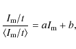
with
By further investigation of the linearity tests with corrected fluxes, we noticed a remaining spatial dependent effect that could not be attributed to the shutter (see Sect. 4.3). This was caused by a smooth pixel-to-pixel variation of the coefficients a and b in the fitted linear relation, which we did not account for. Therefore, the linearity correction was performed for every pixel separately, which improved the photometry by a factor of ten.
![\begin{figure}
\par\includegraphics[width=8.8cm,clip]{13236_lintest.eps} %
\end{figure}](/articles/aa/full_html/2010/07/aa13236-09/img43.png)
|
Figure 3: Linearity test for the CCD of a) OFXB b) Michelbach c) SOAO and d) Vienna. |
| Open with DEXTER | |
Three other cameras also reacted in a non-linear way: the ones at Michelbach Observatory and SOAO show the same discrepancy as OFXB, and the CCD at Vienna Observatory exhibits a higher order effect, but only at low fluxes. We corrected for all these CCD effects.
4.3 Shutter correction
Since the exposure times at the 1.2-m Mercator telescope (ORM) were short, we corrected the images for the shutter effect. As a mechanical shutter needs time to open and close, some regions in the CCD are exposed longer or shorter depending on their position. To quantify and correct for this unwanted effect, we took a similar series of flat fields as needed for the linearity test, only this time with shorter exposure times. If we divided one very short exposure, where the shutter opening and closing time plays an important role by one of the longer exposures, where the shutter effect is negligible, we could actually nicely see the blades of the shutter (see Fig. 4).
![\begin{figure}
\par\includegraphics[width=5cm,clip]{13236_shutter.eps} %
\end{figure}](/articles/aa/full_html/2010/07/aa13236-09/img44.png)
|
Figure 4:
Image showing the calculated |
| Open with DEXTER | |
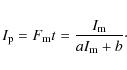
To measure this effect, we handled the problem in the same way as
before, only this time the flux rate was not the variable
parameter, but the exposure time. In the perfect case, the
flux
measured in a given pixel would be

with F again the constant flux rate and t the exposure time. Since at that pixel we have a slightly longer exposure time

By making a linear least-squares fit between this measured flux and the exposure time of the shutter test sequence, we hence obtained the

For all other observing sites except SOAO, the shutter effect was negligible or we could not quantify the effect because of a lack of calibration frames. For SOAO, the correction of the shutter effect was calculated and corrected for in the same way as described above.
4.4 Flat fielding
The final correction applied to the CCD images is flat fielding. It corrects for the pixel-to-pixel sensitivity variations. For every filter and every night, we created a master flat by scaling the flat fields to the normalised level of 1 and taking the mean image while rejecting the extreme values, after checking the flat field's stability by division of one flat by another. Finally the flat field correction was made by dividing the image to be corrected by the master flat. If possible, we took sky flats without tracking (possible stars in the field would then not fall on the same pixels), otherwise dome flats were used. Sometimes we noticed a small difference between dusk and dawn flat fields due to the telescope position. But since we did not dispose of the appropriate calibration frames to correct for it, we took a nightly average. Regions with vignetting on the CCD were trimmed off.
At some observatories, the read-out time of the CCD was very long, so that it was impossible to gather a sufficient number of flat fields in every observed filter per night. In that case, we checked over which time period the flats were stable and combined them together over several nights to construct a master flat. ORM was such an observatory, but the flats from July and August 2006 were not at all stable, caused by the installation of a heat shield in the nitrogen dewar. The flat field change was even noticeable between dusk and dawn and is spatially dependent. Therefore we made a polynomial fit over time for every pixel to interpolate the measured flux variation to gain appropriate flats throughout the night.
5 Reduction to differential light curves
The following sections report on the reduction from the calibrated CCD images to differential light curves, which was conducted for each observatory individually (Sects. 5.1-5.4) and the merging of the data of all sites (Sect. 5.5). The reduction method for the photo-electric data taken at ORM with P7 is described in Rufener (1985,1964). For the reduction of the photo-electric measurements of OAN-SPM, we refer to Poretti & Zerbi (1993) and references therein.
5.1 Flux extraction with Daophot
To extract the magnitudes of the different stars on the frames, we used the DAOPHOT II (Stetson 1987) and ALLSTAR (Stetson & Harris 1988) packages.
As a first step we made an extensive master list of 3165 stars in our total field of view by means of a deep and large frame with the best seeing. For this purpose, we utilised the subroutines FIND and PHOT to search for stars and compute their aperture photometry. Although DAOPHOT handles e.g. pixel defects and cosmic rays, the image was checked to reject false star detections. Then we performed profile photometry. The point-spread function (PSF) consisted of an analytical function (appropriate for the instrument, see Table 2) and an empirical table to adapt the PSF in the best way to the image. In general we allowed this function to vary quadratically over the field. Sufficient PSF stars were chosen with PICK for the derivation of the profile shape with the PS subroutine. Subsequently an iterative process was followed to refine this PSF by subtracting neighbouring stars with the calculated profile by ALLSTAR and generating a new PSF with less blended stars until the PSF converged. At last, ALLSTAR fitted all field stars to achieve the best determined CCD coordinates of each star and to obtain their magnitudes. In the end we subtracted all stars in the frame and inspected the resulting image visually. If we could detect any other stars not contained in our master list, we performed the described procedure again on the subtracted image to include them. In addition, a PSF star list was created by selecting isolated and bright stars uniformly spread over the image. The point-spread function calculation was based on these stars instead of further applying the PICK routine.
To convert the star list from one instrument to another, we made a cubic bivariate polynomial transformation of the CCD coordinates X and Y, based on the coordinates of 20 manually cross-identified stars that are well spread over the field. In this way, we obtained a master star list for each CCD. In order to convert an instrument star list of a certain site to each frame, taking only a shift and small rotation into account was sufficient. To do so, we searched for two pre-selected, well-separated, bright but not saturated stars on the image. As a consequence, the strategy to derive the profile photometry as described above could be automated and was used for the fainter stars. This PSF photometry also had the advantage to provide a precise measure of the FWHM (full-width at half-maximum) of the stars, of the mean sky brightness and of the position of the stars in the field.
For the brightest stars, aperture photometry yielded the most precise results. As in our cluster some stars overlap others, we used the routine NEDA to first subtract neighbour stars PSF-wise before determining the aperture photometry. Multiple apertures ranging from 1 until 4 FWHM in steps of 0.25 FWHM and several background radii were tested for every instrument, the one with the most accurate outcome was applied. We tested that using the same aperture for every star yielded best results and so no further correction is needed since the same amount of light is measured for every star.
Some instruments and telescopes dealt with technical problems resulting in distorted images, and sometimes there was bad tracking during the observations. Sporadically, condensation on the cameras occurred and glows were apparent on the images. The weather was not always ideal either. If the images looked really bad, the automatic reduction procedure failed. If the reduction procedure succeeded, but the resulting photometry was inaccurate or inconsistent, the measurements were rejected in the following stage in which we calculated the differential photometry.
5.2 Multi-differential photometry
Our aim was to quantify the relative light variations of the measured stars with high precision. In this view, multi-differential photometry, which takes advantage of the ensemble of stars in our field of view, is exactly what we needed. Comparing each star with a set of reference stars indeed reduced the effects of extinction, instrumental drifts and other non-stellar noise sources if their fluctuations in time were consistent over the full frame, but it would still contain the variability information we searched for.
For each instrument we applied an iterative algorithm to compute this relative photometry. In an outer loop, the set of reference stars was iteratively optimised, whereas in an inner loop, the light curve for a given set of reference stars was improved. As a starting point, an initial set of reference stars was extracted from a fixed list of bright stars.
The inner loop of the iteration consisted in adapting the
light
curve of the reference stars to gain new mean and smaller standard
deviation estimates. In the first three iterations,
the zero
point for image j was calculated as the
mean of the variation of the reference stars
with

where
In the outer loop, the differential magnitudes mc,j
of all stars were computed as
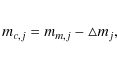
with mm,j the DAOPHOT magnitude of image j and
On average, the final differential photometry was based on 25 reference stars. Images with poor results, where the photometry of the final set of reference stars was used as benchmark, were eliminated at the end. Often this represented 6 to 10% of the total amount of data, but it strongly depended on the instrument.
As a consequence of our choice for bright comparison stars, our approach is optimised for B-type cluster members since they have similar magnitudes and colours as the reference stars. Other stars are typically much fainter, so that their photon noise dominates the uncertainties of the magnitudes.
To improve the overall quality of the data, we removed some outliers with sigma clipping. We used an iterative loop which stops after points were no longer rejected. However, we never discarded several successive measurements as these could originate from an eclipse. Normally the programme converged after a few iterations. The data of the Vienna Observatory (V filter only), Baker Observatory and TUG (T40) were completely rejected since their precision was inferior to the other sites or their photometry was unreliable due to technical problems.
5.3 Error determination
As can be noticed in Table 2, we were dealing with a diverse data set concerning the accuracy. To improve the signal-to-noise (S/N) level in a frequency analysis, it was therefore essential to weight the time series (Handler 2003). In order to have appropriate weights, we aimed at getting error estimates per data point which were as realistic as possible. They had to reflect the quality of the measurements in a time series of a certain instrument and at the same time be intercomparable for the different inhomogenous data sets.
In general it is not easy to make a whole picture of the total error budget. The error derivation of DAOPHOT accounts for the readout noise, photon noise, the flat-fielding error and the interpolation error caused by calculating the aperture and PSF photometry. Besides these, there is also scintillation noise, noise caused by the zero point computation by means of the comparison stars and other CCD-related noise sources depending on the colour of the stars, their position etc. Some analytical expressions to evaluate the most important noise sources are available in the literature (e.g., Kjeldsen & Frandsen 1992).
We preferred to work empirically and determined an error
approximation
together with the relative photometry. We assumed that the standard
deviation of the contribution of each reference star to the calculated
zero point of a certain image j
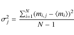
contained all noise sources. For the bright stars, which have a photon noise comparable to the photon noise of the reference stars, we can use this value directly as the noise estimate of image j since
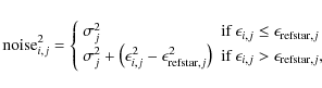
where
We verified if this indeed corresponded to the intercomparable
error
determination we searched for. To this end, we used
the
relation between the noise in the time domain
![]() ,
i.e., the mean measured error of the star computed by us, and the noise
in the frequency domain
,
i.e., the mean measured error of the star computed by us, and the noise
in the frequency domain
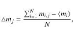
![]() ,
i.e., the amplitude noise in the periodogram, for a given
star i, given by
,
i.e., the amplitude noise in the periodogram, for a given
star i, given by
with N the number of measurements of star i. We checked this correlation for the brightest 300 stars in the field. An example for Bia
![\begin{figure}
\par\includegraphics[width=8.5cm,clip]{13236_errcomp.eps}
\end{figure}](/articles/aa/full_html/2010/07/aa13236-09/img60.png)
|
Figure 5:
Comparison of the mean measured error
|
| Open with DEXTER | |
5.4 Detrending
Even after taking differential photometry, residual trends can
still
exist in the light curves, e.g. due to instrumental drifts or
changes in the atmospheric transparency. As we were also
interested in low frequencies, where the residual trends will cause
high noise levels, we wanted to correct the time series for these
trends. In order to do so, we applied the Sys-Rem algorithm by
Tamuz et al. (2005),
which was specifically
developped to remove correlated noise by searching for linear
systematic effects that are present in the data of a lot of stars. The
algorithm minimises the global expression
where mij and
Sys-Rem used the error on the measurements to downweigh bad measurements. However, we noticed that including faint stars in the sample to also correct bright stars degrades the photometric results of the latter. Hence we only used the whole set of stars to ameliorate the data of the faintest stars, and we used a sub-sample of bright stars for the application of Sys-Rem to the brightest ones. Stars showing clear long-term variability were also excluded from the sample.
The number of effects to be removed is a free parameter in the
algorithm and should be handled with care. Indeed, we wanted to
eliminate as many instrumental trends as possible, but certainly no
stellar variability. For every instrument we examined the periodograms
averaged for the 100 and 300 brightest stars to
evaluate when
sufficient trends are taken out the data. At the same time the
periodograms of the known ![]() Cep stars
were inspected to make sure the known stellar variability was not
affected. An example for Bia
Cep stars
were inspected to make sure the known stellar variability was not
affected. An example for Bia![]() ków Observatory is shown in Fig. 6,
and it can be clearly seen that the accuracy improved.
In most cases, up to three linear systematic effects
were
removed.
ków Observatory is shown in Fig. 6,
and it can be clearly seen that the accuracy improved.
In most cases, up to three linear systematic effects
were
removed.
![\begin{figure}
\par\includegraphics[width=8.8cm,clip]{13236_sysrem.eps}
\end{figure}](/articles/aa/full_html/2010/07/aa13236-09/img63.png)
|
Figure 6:
Periodogram examples from Biaków Observatory to show the impact
of Sys-Rem. a) The average periodogram of
the 300 brightest stars in the field, left:
without detrending, right: with three effects
removed. b) Idem for the known |
| Open with DEXTER | |
5.5 Merging
At this point the individual time series were fully processed and could be joined per filter (U, B, V, I). No phase shifts nor amplitude variations were expected for the data of the various sites for the oscillating B-stars and so only a magnitude shift, which can depend on the star, was computed.
To determine this magnitude shift, we made use of overlapping
observation periods. We started with data from Bia![]() ków
Observatory, which holds the most accurate measurements, and added the
other instruments one by one, beginning with the site that had the most
intervals in common. We smoothed the light curves and interpolated the
data points before calculating the mean shift to account for variations
in the time series. If no measurements were taken at
the same
time, the light curves were just shifted by matching their mean values.
ków
Observatory, which holds the most accurate measurements, and added the
other instruments one by one, beginning with the site that had the most
intervals in common. We smoothed the light curves and interpolated the
data points before calculating the mean shift to account for variations
in the time series. If no measurements were taken at
the same
time, the light curves were just shifted by matching their mean values.
6 Time-series analysis
To obtain the final light curves, the merged data sets were once more sigma-clipped and detrended with Sys-Rem. The final precision for the brightest stars is 5.7 mmag in V, 6.9 mmag in B, 5.0 mmag in I and 5.3 mmag in U. We also eliminated the light curves of about 25% of the stars, since those stars were poorly measured.
Given the better precision in the V filter and the overwhelming number of data points, the search for variable stars and an automated frequency analysis were carried out in this filter. The U-, B-, and I-filter data will be used in subsequent papers which will present a more detailed frequency analysis of the pulsating stars and eclipsing binaries found in our data.
6.1 Detection of variable stars
The following four tools were used to search for variability, whether
periodic or not. First, the standard deviation of the light
curve
gave an impression of the intrinsic variability. However, also the mean
magnitude of the star had to be considered, so that the bright
variable stars with low
amplitudes were selected and not the faint constant stars.
To take
the brightness of the star into account, we calculated the ``relative
standard deviation'' of the light curve, i.e.,
![]() ,
where
,
where ![]() is
the moving average of the bulk of (constant) stars over their
magnitude, as denoted by the grey line in Fig. 7a.
is
the moving average of the bulk of (constant) stars over their
magnitude, as denoted by the grey line in Fig. 7a.
The Abbé test gave another indication of variability.
It depends on the point-to-point variations and is sensible to
the
derivative of the light curve. For a particular star, its
value
was calculated as
where the sum is taken over the different data points. The value of the Abbé test is close to one for constant stars, larger than one for stars that are variable on shorter time scales than the characteristic sampling of the light curve and significantly smaller than one for variability on longer time scales.
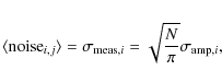
We also determined the reduced ![]() of the light curves
of the light curves
where N is the number of measurements and ei is the error on the magnitude mi, as calculated in Sect. 5.3. Its value expresses to what extent the light curve can be considered to have a constant value, the mean magnitude, and so whether there is or not noticeable variability above the noise level. Diagrams of these four indicators (
![\begin{figure}
\par\includegraphics[width=8.8cm,clip]{13236_vartest.eps}\vspace*{-3mm}
\end{figure}](/articles/aa/full_html/2010/07/aa13236-09/img70.png)
|
Figure 7:
Different diagnostics to detect variability: a) the
standard deviation of the light curve, b) the
relative standard deviation, c) the Abbé
test and
d) the reduced |
| Open with DEXTER | |
A powerful tool to detect periodic variability is frequency analysis. For every star, weighted Lomb-Scargle diagrams (see Sect. 6.2) were calculated from 0 to 50 d-1. As this method assumes sinusoidal variations, phase dispersion minimisation diagrams (Stellingwerf 1978) were computed as well. In these periodograms we searched for significant frequency peaks.
In addition, we searched for variable stars by applying the automated classification software by Debosscher et al. (2007). This code was developed primarily for space data (Debosscher et al. 2009), but was previously also applied to the OGLE database of variables (Sarro et al. 2009).
Furthermore, also visual inspection of the light curves ranging over a couple to tens of days gives a strong indication of variability, especially for the brighter stars. After exploring the different diagnostics for variable star detection, we ended up with a list of about 400 stars that were selected for further analysis.
6.2 Frequency analysis
As a consequence of the large number of (candidate) variable stars, we applied an automatic procedure for the frequency analysis of the V data, which is a common procedure adopted in the classification of variable star work when treating numerous stars (e.g., Debosscher et al. 2009). This approach cannot be optimal for each individual case, and the results have to be regarded in this way. We thus limit ourselves to report on the dominant frequency only in this work (see Table A.1), even though numerous variables are multi-periodic. An optimal and detailed frequency analysis of the multi-periodic pulsators in the cluster will be the subject of a subsequent paper. For a discussion on the spectral window of the data, we refer to Saesen et al. (2009).
Due to changes in observing conditions and instrumentation with different inherent noise levels, there was a large variation in the data quality of the light curve. Following Handler (2003), it was therefore crucial to apply weights when periodograms were computed to suppress bad measurements and enhance the best observing sites. Accordingly, we used the generalised Lomb-Scargle periodogram of Zechmeister & Kürster (2009), where we gave each data point a weight inversely proportional to the square of the error of the measurement: wi=1/ei2. Moreover, this method takes also a floating mean into account besides the harmonic terms in sine and cosine when calculating the Lomb-Scargle fit (Lomb 1976; Scargle 1982). The spectra were computed from 0 d-1 to 50 d-1 in steps of 1/5T, where T is the total time span of the light curve.
In these periodograms, a frequency peak was considered as
significant
when its amplitude was above four times the noise level, i.e.,
a signal-to-noise ratio greater than 4.0 in amplitude
(Breger et al. 1993).
The noise at a certain frequency was calculated as the mean amplitude
of the
subsequent periodogram, i.e., the periodogram of the data prewhitened
for the suspected frequency. The interval over which we evaluated the
average changed according to the frequency value to account for the
increasing noise at lower frequencies: we used an interval of
1 d-1 for
![]() d-1,
of 1.9 d-1 for
d-1,
of 1.9 d-1 for
![]() d-1,
of 3.9 d-1 for
d-1,
of 3.9 d-1 for
![]() d-1
and of 5 d-1 for
d-1
and of 5 d-1 for
![]() d-1.
d-1.
Our strategy for the automatic computations was the following: subsequent frequencies were found by the standard procedure of prewhitening. In up to ten steps of prewhitening, the frequency with the highest amplitude was selected regardless of its S/N, as long as the periodogram contained at least one significant peak. In this way, also residual trends, characterised by low frequencies, and their alias frequencies were removed from the data set, and thus a lower noise level was reached. Starting from the 11th periodogram, peaks with the highest signal-to-noise level were selected. The calculations were stopped once no more significant peaks (S/N > 4) were present in the periodogram. We did not perform an optimisation of the frequency value due to the large calculation time and the excessive number of variables. This can, however, induce the effect of finding almost the same frequency value again after prewhitening.
Since some light curves were not perfectly merged, we adopted
the routine described above, excluding frequencies f=n ![]()
![]() with
with
![]() .
A constant magnitude shift was calculated to put the residuals
of
the different observing sites at the same
mean level, and this shift was then applied to the original data. Then
we repeated this process, now allowing all frequencies. After one more
frequency search, the residuals were sigma-clipped and a last frequency
analysis was carried out.
.
A constant magnitude shift was calculated to put the residuals
of
the different observing sites at the same
mean level, and this shift was then applied to the original data. Then
we repeated this process, now allowing all frequencies. After one more
frequency search, the residuals were sigma-clipped and a last frequency
analysis was carried out.
The results of this period investigation, which was carried out in the best way we could for an automated analysis, are described from Sect. 8 onward. Frequency values that will be used for stellar modelling need to be derived from a detailed, manual and multi-colour analysis of the 185 variable stars, where the frequency derivation schemes will be optimised according to the pulsator type. This will be presented in subsequent papers for the pulsators.
7 Absolute photometry
Absolute photometry of a cluster is a powerful tool to simultaneously determine general cluster parameters like the distance, reddening and age, and stellar parameters for the cluster members like their spectral type and position in the HR diagram. As pointed out in Sect. 2, NGC 884 is a well-studied cluster, but we wanted to take a homogeneous and independent data set of the observed field. As these observations were not directly part of the multi-site campaign, we describe them explicitly together with the specific data reduction and the determination of the cluster parameters. The stellar parameters like cluster membership, effective temperature and gravity, will be deduced and combined with spectroscopy in a subsequent paper.
7.1 Observations and data reduction
During seven nights in December 2008 and January 2009, absolute photometry of NGC 884 was taken with the CCD camera Merope at the Mercator telescope at ORM. Since the FoV of this CCD is small, four slightly overlapping fields were mapped to contain as many field stars observed in the multi-site campaign as possible. The seven Geneva filters U, B1, B, B2, V1, V and G were used in long and short exposures to have enough signal for the fainter stars while not saturating the bright ones. Three to four different measurements spread over different nights were carried out to average out possible variations. The calibration and reduction of these data were performed as described above in Sects. 4 and 5.
In between the measurements of the cluster, Geneva standard stars were observed to account for atmospheric changes. They were carefully chosen over different spectral types and observed at various air masses to quantify the extinction of the night. Because the standard stars were very bright and isolated, they were often defocused, and their light was measured by means of aperture photometry with a large radius. A correction factor, determined by bright isolated cluster stars, was applied to the cluster data to quantify their flux in the same way as the standard stars.
First, the measured magnitudes
![]() were corrected for the exposure time
were corrected for the exposure time
![]() with the formula
with the formula
We then determined the extinction in each night for each filter through the measured and catalogue values (Rufener 1988; Burki 2010) of the standard stars
where k is the extinction coefficient, Fz the airmass of the star and
Despite the effort to match the physical passbands of the
CCD system to the reference photometric system,
a discrepancy
between the observed and catalogue values of the standard stars
emerged. It depended on the colours of the stars and was
partly
due to some flux leakage at red wavelenghts of the camera. Therefore an
additional transformation to the standard Geneva system is needed. Bratschi (1998) studied the
transformation
from the natural to the standard Geneva system based on
CCD measurements of 242 standard stars.
He remarked that
the colour-colour residuals clearly show that the connection between
these two systems is not a simple relation governed by a single colour
index, but rather a relation between the full photometric property of
the stars and residuals. Since using all colour indices may not be the
most robust and simple way for a transformation as the colour indices
are strongly related, he tested whether to use all or a subset
of
indices. Bratschi (1998)
concluded that all indices are needed to remove small local
discrepancies of
the residuals in relation to the different colours, leading to a
significant improvement of the quality of reduction. Following Bratschi (1998), we fitted the
most general linear transform to the data of the standard stars
In this expression, C stands for the six measured Geneva colours on the one hand and the measured V magnitude on the other hand, leading to seven equations in total. The different coefficients aij were determined with a linear least squares fitting and the cluster data were then transformed to the standard system.
In each step described above, we calculated the error propagation. Furthermore, a weighted mean over the different final measurements of each star was taken to average out unwanted variations, leaving us with one final value of the star in each Geneva filter.
7.2 Cluster parameters
A number of photometric diagrams in the Geneva system are appropriate
to study cluster parameters. These include (X,Y),
(X,V),
(B2-V1,B2-U)
and (B2-V1,V),
where X and Y
are the so-called reddening-free parameters. For their definition and
meaning, we refer to Carrier
et al. (1999) and references therein. In Carrier et al. (1999),
the procedures to deduce the reddening, distance and age of the cluster
are explained. We checked the validity of the assumption of uniform
reddening in the cluster. For this purpose, we determined the
reddening
E(B2-V1)
of the cluster with the calibration of Cramer
(1993)
by means of selected B-type cluster members and omitting the known
Be stars, since they are additionally reddened by a
surrounding
disk. The spread in the reddening values was large, having
a peak-to-peak difference of
E(B2-V1)=0.21,
which corresponds to
![]() in the Johnson system
following the relations
in the Johnson system
following the relations
![]() and E(B2-V1)=0.75 E(B-V)
given by Cramer
(1984,1999).
Moreover, these reddening variations seemed not randomly spread over
the cluster, but show instead spatial correlations. Hence
we performed a simulation by randomly permuting the reddening
values and measuring the rate of coordinate dependence by the slopes of
a linear least-squares fit in function of the CCD X
and Y coordinates. This simulation pointed
out that the probability of the correlation to be due to
noise is smaller than 10-5 and so
proved the non-uniformity of the reddening throughout the cluster,
shown in Fig. 8.
and E(B2-V1)=0.75 E(B-V)
given by Cramer
(1984,1999).
Moreover, these reddening variations seemed not randomly spread over
the cluster, but show instead spatial correlations. Hence
we performed a simulation by randomly permuting the reddening
values and measuring the rate of coordinate dependence by the slopes of
a linear least-squares fit in function of the CCD X
and Y coordinates. This simulation pointed
out that the probability of the correlation to be due to
noise is smaller than 10-5 and so
proved the non-uniformity of the reddening throughout the cluster,
shown in Fig. 8.
![\begin{figure}
\par\includegraphics[angle=270,width=8.8cm,clip]{13236_reddening.eps} %
\end{figure}](/articles/aa/full_html/2010/07/aa13236-09/img84.png)
|
Figure 8:
Colour-scale plot of the non-uniform reddening
|
| Open with DEXTER | |
After dereddening all stars by an interpolation of the calibrated
reddening values, we adjusted a zero-age main sequence (ZAMS) (Mermilliod 1981) to the
photometric diagrams, and this hinted at an over-estimation of the
reddening value by ![]() =
0.04
=
0.04 ![]() 0.01 in the Johnson system. The origin of this offset remains
unknown. The ZAMS fitting finally resulted in a distance
estimate
of about 2.2 kpc. To derive the age, we fitted the isochrones
of Schaller et al. (1992)
and Bertelli et al. (1994).
The models of Schaller
et al. (1992)
we used took standard overshooting, a standard mass loss and
solar
metallicity into account, and we used the models of Table 5 of
Bertelli et al. (1994),
suited for solar metallicity. The isochrone fitting lead to
a log age of 7.15
0.01 in the Johnson system. The origin of this offset remains
unknown. The ZAMS fitting finally resulted in a distance
estimate
of about 2.2 kpc. To derive the age, we fitted the isochrones
of Schaller et al. (1992)
and Bertelli et al. (1994).
The models of Schaller
et al. (1992)
we used took standard overshooting, a standard mass loss and
solar
metallicity into account, and we used the models of Table 5 of
Bertelli et al. (1994),
suited for solar metallicity. The isochrone fitting lead to
a log age of 7.15 ![]() 0.15 where part of the error is due to
systematic differences among the theoretical models. Figure 9 denotes the
dereddened and extinction corrected colour-magnitude
(B2-V1,V)-diagram,
showing a set of isochrones. All the derived values agree well with the
literature values mentioned in Sect. 2.
0.15 where part of the error is due to
systematic differences among the theoretical models. Figure 9 denotes the
dereddened and extinction corrected colour-magnitude
(B2-V1,V)-diagram,
showing a set of isochrones. All the derived values agree well with the
literature values mentioned in Sect. 2.
![\begin{figure}
\par\includegraphics[width=8.5cm,clip]{13236_hr.eps}\vspace*{-3mm}
\end{figure}](/articles/aa/full_html/2010/07/aa13236-09/img86.png)
|
Figure 9: Dereddened and extinction corrected colour-magnitude (B2-V1,V)-diagram, showing four isochrones: two for log age = 7.1 and 7.2 from Schaller et al. (1992) in blue and two for the same age from Bertelli et al. (1994) in green. |
| Open with DEXTER | |
8 Variable stars
For the discussion below we divided the variable stars according to their spectral type, determined by the absolute photometry, which was taken for all stars in a homogeneous and consistent way. Thanks to the design of the Geneva small band filters, B2-V1 is an excellent effective temperature indicator, and the orthogonal reddening-free parameters X and Y show the spectral type of a star, whether it belongs to the cluster or not (Kunzli et al. 1997). If no absolute photometry was available for the star of interest, (V-I,V)- and (B-V,V)-diagrams based on relative photometry were inspected. We also compared literature values for spectral types with the outcome of our photometric diagrams. Further, we classify the stars by their observed variability behaviour: multi-periodic, mono-periodic (possibly with the presence of harmonics) or irregular. The eclipsing binaries are treated in a separate subsection.
All figures for the discovered variable stars can be found in the electronic Appendix A, where we show for each star the V light curve, a phase plot folded with the main frequency, the photometric diagrams, the window function and the generalised Lomb-Scargle diagrams in the different steps of subsequent prewhitening in the V-filter. Each separate category of variables will be described here with some typical and atypical examples. For an extensive overview of the properties of the known classes of pulsating stars, we refer to Chapter 2 of Aerts et al. (2009).
Below we adopted a numbering scheme to discuss the stars. Cross referencing to WEBDA numbering (http://www.univie.ac.at/webda/), which is based on the Oosterhoff (1937) numbering and extended to include additional stars coming from other studies, is available in Table A.1 in the electronic Appendix A. This table also contains an overview of the coordinates of the star, its spectral type, its mean Geneva V, B2-V1 and B2-U photometry and its main frequency and amplitude. We recall that we do not list all the frequencies found from the automated analysis in Table A.1. We will provide the final frequencies from a detailed analysis tuned to the various types of pulsators, which may be slightly different from those found here, in a follow-up paper for further use in stellar modelling.
8.1 Variable B-type stars
8.1.1 Multi-periodic B-type stars
Figures showing the multi-periodic B-type stars can be found in the
electronic Appendix A
as Figs. A.1-A.72. The
classical multi-periodic B-type stars are ![]() Cep and
SPB stars.
Cep and
SPB stars. ![]() Cep
stars are early B-type stars showing p-modes with frequency values
ranging from 3 to 12 d-1.
SPB stars are later B-type stars exciting g-modes with lower
frequencies from 0.3 to 1 d-1.
Hybrid B-pulsators, showing at the same time p- and g-modes,
also exist.
Cep
stars are early B-type stars showing p-modes with frequency values
ranging from 3 to 12 d-1.
SPB stars are later B-type stars exciting g-modes with lower
frequencies from 0.3 to 1 d-1.
Hybrid B-pulsators, showing at the same time p- and g-modes,
also exist.
A typical new ![]() Cep
star is the early-B star 00011, where we observed three
independent frequencies, f1=4.582 d-1,
f2=5.393 d-1
and f5=4.449 d-1
and one harmonic frequency, f4=2
f1
(see Figs. 10, 11). We have to
be careful with the interpretation of frequency f3=1.053 d-1:
although it deviates more than the resolution (0.001 d-1)
from 1.003 d-1, the application of
Sys-Rem can have enhanced this difference.
Cep
star is the early-B star 00011, where we observed three
independent frequencies, f1=4.582 d-1,
f2=5.393 d-1
and f5=4.449 d-1
and one harmonic frequency, f4=2
f1
(see Figs. 10, 11). We have to
be careful with the interpretation of frequency f3=1.053 d-1:
although it deviates more than the resolution (0.001 d-1)
from 1.003 d-1, the application of
Sys-Rem can have enhanced this difference.
![\begin{figure}
\par\includegraphics[width=8cm,clip]{13236_00011.lc.eps}\vspace*{...
...space*{1mm}
\includegraphics[width=8.5cm,clip]{13236_00011.abs.eps}
\end{figure}](/articles/aa/full_html/2010/07/aa13236-09/img87.png)
|
Figure 10: Light curve ( top), phase plot ( middle) and photometric diagrams ( bottom) of star 00011. The light curve and phase plot are made from the V-filter observations and the different colours denote the different observing sites: ORM - orange, OFXB - dark pink, Michelbach - light blue, Biaków - yellow, Athens - light pink, EUO - dark blue, TUG - brown, Xinglong - green and SOAO - purple. The phase plot is folded with the main frequency, denoted in the X-label and whose value is listed in Table A.1. The different colours in the photometric diagrams indicate the spectral types: B0-B2.5 - dark blue, B2.5-B9 - light blue, A - green, F0-F2 - yellow, F3-F5 - orange, F6-G - red, K-M - brown. The big dot with error bars shows the position of star 00011 in these figures. |
| Open with DEXTER | |
![\begin{figure}
\par\includegraphics[width=8cm,clip]{13236_00011.per.eps} %
\vspace*{-3mm}
\end{figure}](/articles/aa/full_html/2010/07/aa13236-09/img88.png)
|
Figure 11: Frequency analysis for star 00011. We show the window function ( top) and the generalised Lomb-Scargle periodograms in the different steps of subsequent prewhitening in the V-filter. The detected frequencies are marked by a yellow band, the red line corresponds to the noise level and the orange line to the S/N=4 level. |
| Open with DEXTER | |
A typical SPB star is star 02320 (Figs. A.63, A.64). This star has three significant frequencies: f1=0.883 d-1, f2=0.964 d-1 and f3=1.284 d-1.
We also found stars exciting p- and g-modes simultaneously.
For example star 00030 (Figs. A.15, A.16) has two
low frequencies f1=0.340 d-1
and f2=0.269 d-1,
which are typical values for SPB-type pulsations, and it shows one
frequency in the ![]() Cep
star range: f4=7.189 d-1,
while f3=0.994 d-1
is again too close to 1.003 d-1 to be
accepted as intrinsic to the star.
Cep
star range: f4=7.189 d-1,
while f3=0.994 d-1
is again too close to 1.003 d-1 to be
accepted as intrinsic to the star.
We also found some anomalies in the typical classification of
variable
B-stars. First of all, star 02320 is actually the only
SPB candidate in the multi-periodic B-star sample. All other
later
B-type stars exhibit pulsations with higher frequency values than
expected, e.g. the intrinsic frequencies of late-B
star 00183
(Figs. A.47, A.48) are f1=3.680 d-1
and f2=3.904 d-1,
which fall in the interval of ![]() Cep
frequencies. This can however also be a rapidly rotating
SPB star,
since rotation can induce significant frequency shifts for
low-frequency g-modes. However, it could also be a member of a
new
class of low-amplitude pulsators bridging the red edge of the
SPB strip and the blue edge of the
Cep
frequencies. This can however also be a rapidly rotating
SPB star,
since rotation can induce significant frequency shifts for
low-frequency g-modes. However, it could also be a member of a
new
class of low-amplitude pulsators bridging the red edge of the
SPB strip and the blue edge of the ![]() Sct strip,
as recently found from CoRoT data by Degroote et al. (2009a).
Sct strip,
as recently found from CoRoT data by Degroote et al. (2009a).
Another peculiar star is star 00024 (Figs. A.11, A.12),
an early Be-star that revealed two significant frequencies
that are low for classical ![]() Cep
pulsations: f1 = 1.569 d-1
and f4 = 1.777 d-1.
The frequencies are also rather high to be of the SPB class.
The
phase behaviour looks different from a simple sine wave: looking at
other known Be stars, this behaviour seems quite typical for
these
stars, since frequencies and/or amplitudes may change over time as
recently found from uninterrupted CoRoT photometry (e.g., Neiner
et al. 2009; Huat et al. 2009).
Cep
pulsations: f1 = 1.569 d-1
and f4 = 1.777 d-1.
The frequencies are also rather high to be of the SPB class.
The
phase behaviour looks different from a simple sine wave: looking at
other known Be stars, this behaviour seems quite typical for
these
stars, since frequencies and/or amplitudes may change over time as
recently found from uninterrupted CoRoT photometry (e.g., Neiner
et al. 2009; Huat et al. 2009).
Star 02451 (Figs. A.69, A.70) showed
clear variations around 25 and 29 d-1,
frequency values we would expect for ![]() Sct stars.
Because of its B-star appearance in the photometric diagrams, the star
is therefore probably no cluster member.
Sct stars.
Because of its B-star appearance in the photometric diagrams, the star
is therefore probably no cluster member.
8.1.2 Mono-periodic B-type stars
The figures of the frequency analysis for mono-periodic B-type stars can be found in the electronic Appendix A in Figs. A.73-A.150. For the mono-periodic cases, the same nature of pulsations as described above is also observed. However, because we did not find more than one independent frequency, we cannot be sure that the variations are caused by oscillations. Possibilities like spotted stars or ellipsoidal binaries cannot be ruled out, especially if we also deduce harmonics.
Star 00082 (Figs. A.95, A.96) is a typical example: f1 = 0.639 d-1 and f2 = 2 f1 and the phase plot folded with the main frequency is therefore clearly not sinusoidal. Because of the high amplitude of f1, it is possible that we are dealing with non-sinusoidal SPB-oscillations, but it could also be a spot.
In this sample we also have some B-type supergiants that vary
with SPB-type periods. These were originally discovered by Waelkens et al. (1998)
in the Hipparcos mission and were studied in detail
by Lefever et al. (2007).
For instance, star 00008 (Figs. A.75, A.76),
is listed as B2I supergiant (Slesnick
et al. 2002) and has one clear frequency at f2=0.211 d-1.
Possibly ![]() is also present, which is not so surprising since the oscillations of
supergiant stars are often non-sinusoidal.
is also present, which is not so surprising since the oscillations of
supergiant stars are often non-sinusoidal.
8.1.3 Irregular B-type stars
For some stars, the automatic frequency analysis failed, since long-term trends dominate the light curves. This is the case for Be stars that undergo an outburst. For instance, the light curve of star 00009 (Fig. 12) revealed a huge outburst in the beginning of the second observing season and a smaller one in the third observing season. Smaller variations are possibly still hidden in the time series, but a more detailed analysis should point this out.
| Figure 12: Light curve of Be-star 00009, showing outbursts. The different colours denote the different observing sites as in Fig. 10, the light brown data come from the Vienna Observatory. |
|
| Open with DEXTER | |
Other Be stars without significant frequencies do not always show an outburst, but frequency and/or amplitude changes prevented us from detecting the frequency values. Zooms of the light curve sometimes show clear periodicity on time-scales of several hours. Their light curves and some zooms are shown in Figs. A.152-A.159. Star 00003 behaves in the same way (see Fig. A.151), but is not known to be a Be star.
8.2 A- and F-type stars
8.2.1 Multi-periodic A- and F-type stars
Figures showing the multi-periodic A- and F-type stars can be found in
Figs. A.160-A.197 of the
electronic Appendix A.
These
stars are probably ![]() Sct
stars, exciting p-modes with frequencies ranging from 4 d-1
to 50 d-1 or
Sct
stars, exciting p-modes with frequencies ranging from 4 d-1
to 50 d-1 or ![]() Dor stars with
g-modes in the frequency interval from 0.2 d-1to 3 d-1.
Dor stars with
g-modes in the frequency interval from 0.2 d-1to 3 d-1.
For example, A-type star 00315 (Figs. A.168, A.169) shows two
significant ![]() Sct frequencies
f1=35.337 d-1
and f4=21.123 d-1.
F-type star 00371 (Figs. A.180, A.181) shows
four distinct
Sct frequencies
f1=35.337 d-1
and f4=21.123 d-1.
F-type star 00371 (Figs. A.180, A.181) shows
four distinct ![]() Dor frequencies
between 0.243 d-1 and 1.083 d-1.
Dor frequencies
between 0.243 d-1 and 1.083 d-1.
As for the B-type stars, hybrid pulsators showing both p- and g-modes were also discovered among the A-F type stars. F-type star 00187 (Figs. A.160, A.161) could be such a star. After prewhitening for f1=1.888 d-1 and f2=0.983 d-1, the higher frequencies f5=8.135 d-1 and f11=42.565 d-1 appeared.
An interesting case is A-star 00344 (Figs. A.174, A.175).
In this star we observed the frequencies f1=0.840 d-1
and f2=0.875 d-1,
which are too low for
a ![]() Sct star.
These periodicities could be of SPB or
Sct star.
These periodicities could be of SPB or ![]() Dor
nature, but following the absolute photometry, the star's spectral type
is incompatible with this. The same holds for the star 00577
(Figs. A.230, A.231). Here the
photometric diagrams indicated
that this is an F-star, but the periodogram shows a higher
frequency value than for the
Dor
nature, but following the absolute photometry, the star's spectral type
is incompatible with this. The same holds for the star 00577
(Figs. A.230, A.231). Here the
photometric diagrams indicated
that this is an F-star, but the periodogram shows a higher
frequency value than for the ![]() Dor pulsators: f3=8.258 d-1.
Dor pulsators: f3=8.258 d-1.
8.2.2 Mono-periodic A- and F-type stars
Mono-periodic ![]() Sct
and
Sct
and ![]() Dor
stars also exist. The
Dor
stars also exist. The ![]() Sct stars
can be unambiguously separated from rotating variables on the basis of
their short periods, while
Sct stars
can be unambiguously separated from rotating variables on the basis of
their short periods, while ![]() Dor stars cannot,
due to their longer periods. All examples can be found in
Figs. A.198-A.245. We remark
that no harmonics were found for the
mono-periodic A-type stars.
Dor stars cannot,
due to their longer periods. All examples can be found in
Figs. A.198-A.245. We remark
that no harmonics were found for the
mono-periodic A-type stars.
8.3 Other variable stars
Besides stars with another spectral type than B, A or F, stars for which the spectral type is uncertain or where no information on this is at our disposal are also treated in this subsection. Their frequency analyses are summarised in Figs. A.246-A.285 for the multi-periodic stars and in Figs. A.286-A.325 for the mono-periodic stars. Using the frequency values alone, it seems not possible to reliably classify the stars.
For the main-sequence G-type stars we only expected solar-like oscillations, spots, or ellipsoidal binaries, but we had some cases with a few close frequency values and sometimes nearly a harmonic frequency. For example star 00681 (Figs. A.252, A.253) has the significant frequencies f1=1.818 d-1 and f2=1.808 d-1. This is probably a sign of bad prewhitening since we did not optimise the frequency value before prewhitening.
In addition, six irregular variable stars were also found. They are listed as supergiants in SIMBAD: 00001 (M4I), 00002 (B2I), 02427 (M1I), 02428 (M1I) and 03165 (A2I), except 03164 (sdM1). However, the spectral type of star 03164 is probably wrong in SIMBAD, and this star is listed as M0I supergiant in Slesnick et al. (2002). For these stars we avoid to show the photometric diagrams, since the values are uncertain. For completeness, we do show the light curves and some zooms in Figs. A.326-A.331.
8.4 Eclipsing binaries
Apart from the two known cases announced in Krzesinski & Pigulski (1997), we discovered six new and four candidate eclipsing binaries. Classical frequency analysis methods did not succeed to find their periods, so we estimated them from the eclipse minima and by visual inspection of the phase plots. The star numbers of the confirmed eclipsing binaries together with their periods are given in Table 3. Their phase plots can be found in the electronic Appendix A in Figs. A.332-A.339. The four candidate eclipsing binaries, stars 00033, 00045, 00110 and 00316, show dips in their light curves that could point to an eclipse. Extracts of these parts of their light curve are shown in Figs. A.340-A.343. A separate paper including long-term spectroscopy is in preparation and is devoted to star 00010 (Southworth et al., in preparation), while the other eclipsing binaries we discovered will be modelled together in a subsequent paper. The studies on these eclipsing binaries will be performed to deduce more cluster characteristics, which will serve as input for any future modelling.
Table 3: The (candidate) eclipsing binaries.
9 Summary and conclusion
We have carried out an extensive multi-site campaign to gather time-resolved multi-colour CCD photometry of a field of the open cluster NGC 884. The aim was to search for variable stars, in particular B-type pulsators. In total, an international team consisting of 61 observers used 15 different instruments attached to 13 telescopes to collect almost 77 500 CCD images and 92 h of photo-electric data in U, B, V and I filters.
We performed the calibration of the CCD images by standard bias and dark subtractions, non-linearity and shutter corrections and flat fielding. We extracted the fluxes of the stars with the DAOPHOT II (Stetson 1987) and ALLSTAR (Stetson & Harris 1988) packages, in which we combined PSF and aperture photometry. We applied multi-differential photometry to correct for atmospheric extinction and detrended the data sets with the Sys-Rem algorithm by Tamuz et al. (2005). We succeeded in deducing realistic and inter-comparable error estimates for the measurements. For the brightest stars, we obtained an overall V accuracy of 5.7 mmag, 6.9 mmag in B, 5.0 mmag in I and 5.3 mmag in U.
The search for variable stars among the 3165 observed
stars was
based on several indicators like the standard deviation of the light
curve, the Abbé test, the reduced ![]() value, frequency analysis and visual inspection. About
400 candidate variable stars were subjected to an automated
weighted frequency analysis revealing 36 multi-periodic and
39 mono-periodic B-stars, 19 multi-periodic and
24 mono-periodic A- and F-stars and 20 multi-periodic
and
20 mono-periodic variable stars of unknown nature. Moreover,
15 irregular variable stars were found, of which
eight are
Be stars and six (super)giant stars. We also detected, apart
from
two known cases, six new and four candidate eclipsing binaries.
value, frequency analysis and visual inspection. About
400 candidate variable stars were subjected to an automated
weighted frequency analysis revealing 36 multi-periodic and
39 mono-periodic B-stars, 19 multi-periodic and
24 mono-periodic A- and F-stars and 20 multi-periodic
and
20 mono-periodic variable stars of unknown nature. Moreover,
15 irregular variable stars were found, of which
eight are
Be stars and six (super)giant stars. We also detected, apart
from
two known cases, six new and four candidate eclipsing binaries.
The interpretation of these variable stars is not always
straightforward and needs further investigation. In general,
it seems that we cannot rely anymore on the simple
classification
of B-type stars by means of the theoretical instability domains for ![]() Cep
and SPB stars as in e.g. Miglio
et al. (2007). This was also pointed out by Degroote et al. (2009a)
based on their analysis of B-type stars in the CoRoT exoplanet field
data. We arrive at the same conclusions, derived from an independent
data set with totally different characteristics: numerous stars have
frequency
ranges extending from the gravity-mode range corresponding to periods
of days to the pressure-mode regime corresponding to periods of a few
hours. A part of the anomalies in the classical categorisation
can
be explained by rotation, since, as discussed in
Sect. 2,
it is well known that the average rotational velocities for
the brightest stars in this cluster is high (Slettebak
1968)
and this affects the observed frequency values. However, the
complication probably also arises because both the CoRoT data
and
our cluster data exceed the previous data sets of B-type pulsators by
far in terms of number of targets and photometric precision in the
amplitude spectra. We have thus lowered the threshold of finding new
low-amplitude pulsators, and these seem to come in more flavours than
anticipated so far.
Cep
and SPB stars as in e.g. Miglio
et al. (2007). This was also pointed out by Degroote et al. (2009a)
based on their analysis of B-type stars in the CoRoT exoplanet field
data. We arrive at the same conclusions, derived from an independent
data set with totally different characteristics: numerous stars have
frequency
ranges extending from the gravity-mode range corresponding to periods
of days to the pressure-mode regime corresponding to periods of a few
hours. A part of the anomalies in the classical categorisation
can
be explained by rotation, since, as discussed in
Sect. 2,
it is well known that the average rotational velocities for
the brightest stars in this cluster is high (Slettebak
1968)
and this affects the observed frequency values. However, the
complication probably also arises because both the CoRoT data
and
our cluster data exceed the previous data sets of B-type pulsators by
far in terms of number of targets and photometric precision in the
amplitude spectra. We have thus lowered the threshold of finding new
low-amplitude pulsators, and these seem to come in more flavours than
anticipated so far.
Earlier variability studies on NGC 884 showed the
detection of only very few B-type pulsators: there are two confirmed
and two candidate ![]() Cep
star s in the cluster (see Sect. 2). Waelkens et al. (1990)
and Pigulski et al.
(2001)
were puzzled by this fact, since NGC 884 has roughly the same
age
as NGC 3293, the southern open cluster which yields most known
Cep
star s in the cluster (see Sect. 2). Waelkens et al. (1990)
and Pigulski et al.
(2001)
were puzzled by this fact, since NGC 884 has roughly the same
age
as NGC 3293, the southern open cluster which yields most known
![]() Cep stars
(Stankov & Handler 2005).
Waelkens et al. (1990)
proposed that these observations lend support to the old idea that
large rotational velocities tend to be incompatible with the
Cep stars
(Stankov & Handler 2005).
Waelkens et al. (1990)
proposed that these observations lend support to the old idea that
large rotational velocities tend to be incompatible with the ![]() Cep
phenomenon. Pigulski
et al. (2001)
speculated that the metallicity gradient in the Galaxy may be
responsible for this difference. Our data set revealed
36 multi-periodic and
39 mono-periodic B-type variables, so the lack of
detection
of these oscillators in the past was maybe an observational constraint
due to limited precision and field-of-view, as well as to
short
time bases and too low duty cycles, certainly when noting that most
amplitudes of the variations we detect are low.
Cep
phenomenon. Pigulski
et al. (2001)
speculated that the metallicity gradient in the Galaxy may be
responsible for this difference. Our data set revealed
36 multi-periodic and
39 mono-periodic B-type variables, so the lack of
detection
of these oscillators in the past was maybe an observational constraint
due to limited precision and field-of-view, as well as to
short
time bases and too low duty cycles, certainly when noting that most
amplitudes of the variations we detect are low.
We identified periodic changes in several Be stars. We also
noticed that their phase plot is quite chaotic: it shows more
scatter around the mean light curve in comparison with other pulsating
stars with the same brightness (e.g., ![]() Cep
stars). It could originate from frequencies and/or amplitudes
that
change over time. Some other periodically varying B-type stars have the
same photometric behaviour, suggesting a similar Be nature,
although we do not have direct spectroscopic evidence. This erratic
behaviour in the phase plot was already pointed out by Jerzykiewicz et al.
(2003).
These findings on Be pulsators again fully agree with recent
results from the CoRoT mission, where outbursts could be
interpreted as beating between pressure- and
gravity-modes with time dependent amplitudes (e.g., Neiner
et al. 2009; Huat et al. 2009).
Cep
stars). It could originate from frequencies and/or amplitudes
that
change over time. Some other periodically varying B-type stars have the
same photometric behaviour, suggesting a similar Be nature,
although we do not have direct spectroscopic evidence. This erratic
behaviour in the phase plot was already pointed out by Jerzykiewicz et al.
(2003).
These findings on Be pulsators again fully agree with recent
results from the CoRoT mission, where outbursts could be
interpreted as beating between pressure- and
gravity-modes with time dependent amplitudes (e.g., Neiner
et al. 2009; Huat et al. 2009).
In a subsequent paper we will perform a manual and more
detailed
frequency analysis of the pulsators, especially the B-type stars. For
the moment we did not find clear connections between the dominant
frequency and various observed properties of the stars, but we will
come back on this issue once we studied the different classes of
variable stars in detail. After a detailed frequency analysis we can
also take all detected frequencies into account, instead of only the
dominant one which is treated in this paper. A mode
identification
will also be carried out based on the multi-colour photometry,
to determine the degree ![]() of the oscillations. The eclipsing binaries will be treated as well in
more detail in another paper to deduce more cluster characteristics.
Hereafter, an asteroseismic modelling of the pulsators in the cluster
will be performed, assuming that they have the same age and that they
had the same chemical composition at birth since they were born out of
the same cloud. Given the numerous B-type pulsators discovered in this
cluster, an in-depth evaluation of the stellar evolution
models
seems very promising.
of the oscillations. The eclipsing binaries will be treated as well in
more detail in another paper to deduce more cluster characteristics.
Hereafter, an asteroseismic modelling of the pulsators in the cluster
will be performed, assuming that they have the same age and that they
had the same chemical composition at birth since they were born out of
the same cloud. Given the numerous B-type pulsators discovered in this
cluster, an in-depth evaluation of the stellar evolution
models
seems very promising.
The research leading to these results has received funding from the European Research Council under the European Community's Seventh Framework Programme (FP7/2007-2013)/ERC grant agreement No. 227224 (PROSPERITY), from the Research Council of K.U.Leuven grant agreement GOA/2008/04, from the Fund for Scientific Research of Flanders grant G.0332.06 and from the European Helio- and Asteroseismology Network (HELAS), a major international collaboration funded by the European Commission's Sixth Framework Programme. A.P., G.M. and Z.K. were supported by the NN203 302635 grant from the MNiSW. K.U. acknowledges financial support from a European Community Marie Curie Intra-European Fellowship, contract number MEIF-CT-2006-024476. This research has made use of the WEBDA database, operated at the Institute for Astronomy of the University of Vienna as well as NASA's Astrophysics Data System and the SIMBAD database, operated at CDS, Strasbourg, France.
Note added in proof.
After acceptance of our paper, we became aware of a new stellar
population study of ![]() Persei
based on photometric and
spectroscopic data of numerous cluster members, among which several of
our target stars. This study is of relevance for the follow-up papers
we
have planned. We refer the reader to Thayne et al. (2010, ApJS, 186,
191)
for the results of this interesting study which is complementary to
ours.
Persei
based on photometric and
spectroscopic data of numerous cluster members, among which several of
our target stars. This study is of relevance for the follow-up papers
we
have planned. We refer the reader to Thayne et al. (2010, ApJS, 186,
191)
for the results of this interesting study which is complementary to
ours.
References
- Aerts, C., Thoul, A., Daszynska, J., et al. 2003, Science, 300, 1926 [NASA ADS] [CrossRef] [PubMed] [Google Scholar]
- Aerts, C., Christensen-Dalsgaard, J., & Kurtz, D. W. 2009, Asteroseismology (Springer) [Google Scholar]
- Ausseloos, M., Scuflaire, R., Thoul, A., & Aerts, C. 2004, MNRAS, 355, 352 [NASA ADS] [CrossRef] [Google Scholar]
- Balona, L. A. 1994, MNRAS, 267, 1060 [NASA ADS] [CrossRef] [Google Scholar]
- Bertelli, G., Bressan, A., Chiosi, C., Fagotto, F., & Nasi, E. 1994, A&AS, 106, 275 [NASA ADS] [Google Scholar]
- Bratschi, P. 1998, Ph.D. Thesis, Geneva Observatory, Switzerland [Google Scholar]
- Breger, M., Stich, J., Garrido, R., et al. 1993, A&A, 271, 482 [NASA ADS] [Google Scholar]
- Briquet, M., Lefever, K., Uytterhoeven, K., & Aerts, C. 2005, MNRAS, 362, 619 [NASA ADS] [CrossRef] [Google Scholar]
- Briquet, M., Morel, T., Thoul, A., et al. 2007, MNRAS, 381, 1482 [NASA ADS] [CrossRef] [Google Scholar]
- Burki, G. 2010, http://obswww.unige.ch/gcpd/ph13.html [Google Scholar]
- Capilla, G., & Fabregat, J. 2002, A&A, 394, 479 [NASA ADS] [CrossRef] [EDP Sciences] [Google Scholar]
- Carrier, F., Burki, G., & Richard, C. 1999, A&A, 341, 469 [Google Scholar]
- Cramer, N. 1984, A&A, 132, 283 [NASA ADS] [Google Scholar]
- Cramer, N. 1993, A&A, 269, 457 [NASA ADS] [Google Scholar]
- Cramer, N. 1999, New Astron. Rev., 43, 343 [NASA ADS] [CrossRef] [Google Scholar]
- Daszynska-Daszkiewicz, J., Dziembowski, W. A., & Pamyatnykh, A. A. 2005, A&A, 441, 641 [NASA ADS] [CrossRef] [EDP Sciences] [Google Scholar]
- Debosscher, J., Sarro, L. M., Aerts, C., et al. 2007, A&A, 475, 1159 [NASA ADS] [CrossRef] [EDP Sciences] [Google Scholar]
- Debosscher, J., Sarro, L. M., López, M., et al. 2009, A&A, 506, 519 [NASA ADS] [CrossRef] [EDP Sciences] [Google Scholar]
- Degroote, P., Aerts, C., Ollivier, M., et al. 2009a, A&A, 506, 471 [NASA ADS] [CrossRef] [EDP Sciences] [Google Scholar]
- Degroote, P., Briquet, M., Catala, C., et al. 2009b, A&A, 506, 111 [NASA ADS] [CrossRef] [EDP Sciences] [Google Scholar]
- Desmet, M., Briquet, M., Thoul, A., et al. 2009, MNRAS, 396, 1460 [NASA ADS] [CrossRef] [MathSciNet] [Google Scholar]
- Dziembowski, W. A., & Pamyatnykh, A. A. 2008, MNRAS, 385, 2061 [NASA ADS] [CrossRef] [Google Scholar]
- Handler, G. 2003, Baltic Astron., 12, 253 [Google Scholar]
- Handler, G., Shobbrook, R. R., & Mokgwetsi, T. 2005, MNRAS, 362, 612 [NASA ADS] [CrossRef] [Google Scholar]
- Handler, G., Jerzykiewicz, M., Rodríguez, E., et al. 2006, MNRAS, 365, 327 [NASA ADS] [CrossRef] [Google Scholar]
- Handler, G., Tuvikene, T., Lorenz, D., et al. 2007, Commun. Asteroseismol., 150, 193 [NASA ADS] [CrossRef] [Google Scholar]
- Handler, G., Tuvikene, T., Lorenz, D., et al. 2008, Commun. Asteroseismol., 157, 315 [NASA ADS] [Google Scholar]
- Handler, G., Matthews, J. M., Eaton, J. A., et al. 2009, ApJ, 698, L56 [NASA ADS] [CrossRef] [Google Scholar]
- Huat, A., Hubert, A., Baudin, F., et al. 2009, A&A, 506, 95 [NASA ADS] [CrossRef] [EDP Sciences] [Google Scholar]
- Jerzykiewicz, M., Kopacki, G., Molenda-Zakowicz, J., & Ko▯aczkowski, Z. 2003, Acta Astron., 53, 151 [NASA ADS] [Google Scholar]
- Keller, S. C., Grebel, E. K., Miller, G. J., & Yoss, K. M. 2001, AJ, 122, 248 [NASA ADS] [CrossRef] [Google Scholar]
- Kjeldsen, H., & Frandsen, S. 1992, PASP, 104, 413 [NASA ADS] [CrossRef] [Google Scholar]
- Ko▯aczkowski, Z., Pigulski, A., Kopacki, G., & Michalska, G. 2004, Acta Astron., 54, 33 [NASA ADS] [Google Scholar]
- Krzesinski, J. 1998, in A Half Century of Stellar Pulsation Interpretation, ed. P. A. Bradley, & J. A. Guzik, ASP Conf. Ser., 135, 157 [Google Scholar]
- Krzesinski, J., & Pigulski, A. 1997, A&A, 325, 987 [NASA ADS] [Google Scholar]
- Krzesinski, J., & Pigulski, A. 2000, in The Impact of Large-Scale Surveys on Pulsating Star Research, ed. L. Szabados, & D. Kurtz, IAU Colloq., 176, ASP Conf. Ser., 203, 496 [Google Scholar]
- Kunzli, M., North, P., Kurucz, R. L., & Nicolet, B. 1997, A&AS, 122, 51 [NASA ADS] [CrossRef] [EDP Sciences] [Google Scholar]
- Lefever, K., Puls, J., & Aerts, C. 2007, A&A, 463, 1093 [NASA ADS] [CrossRef] [EDP Sciences] [Google Scholar]
- Lomb, N. R. 1976, Ap&SS, 39, 447 [NASA ADS] [CrossRef] [Google Scholar]
- Malchenko, S. L. 2007, in 14th Young Scientists Conference on Astronomy and Space Physics, ed. G. Ivashchenko, & A. Golovin, 59 [Google Scholar]
- Malchenko, S. L., & Tarasov, A. E. 2008, ApJ, 51, 250 [Google Scholar]
- Marco, A., & Bernabeu, G. 2001, A&A, 372, 477 [NASA ADS] [CrossRef] [EDP Sciences] [Google Scholar]
- Mazumdar, A., Briquet, M., Desmet, M., & Aerts, C. 2006, A&A, 459, 589 [NASA ADS] [CrossRef] [EDP Sciences] [Google Scholar]
- Mermilliod, J. C. 1981, A&A, 97, 235 [NASA ADS] [Google Scholar]
- Miglio, A., Montalbán, J., & Dupret, M.-A. 2007, MNRAS, 375, L21 [NASA ADS] [CrossRef] [Google Scholar]
- Neiner, C., Gutiérrez-Soto, J., Baudin, F., et al. 2009, A&A, 506, 143 [NASA ADS] [CrossRef] [EDP Sciences] [Google Scholar]
- Oosterhoff, P. T. 1937, Annalen van de Sterrewacht te Leiden, 17, 1 [Google Scholar]
- Pamyatnykh, A. A., Handler, G., & Dziembowski, W. A. 2004, MNRAS, 350, 1022 [NASA ADS] [CrossRef] [Google Scholar]
- Percy, J. R. 1972, PASP, 84, 420 [NASA ADS] [CrossRef] [Google Scholar]
- Pigulski, A. 2008, J. Phys. Conf. Ser., 118, 012011 [NASA ADS] [CrossRef] [Google Scholar]
- Pigulski, A., Handler, G., Michalska, G., et al. 2007, Commun. Asteroseismol., 150, 191 [NASA ADS] [CrossRef] [Google Scholar]
- Pigulski, A., Kopacki, G., & Ko▯aczkowski, Z. 2001, Acta Astron., 51, 159 [NASA ADS] [Google Scholar]
- Poretti, E., & Zerbi, F. 1993, A&A, 268, 369 [NASA ADS] [Google Scholar]
- Rufener, F. 1964, Publ. Obs. Genève, Ser. A, 66, 413 [Google Scholar]
- Rufener, F. 1985, in Calibration of Fundamental Stellar Quantities, ed. D. S. Hayes, L. E. Pasinetti, & A. G. D. Philip, IAU Symp., 111, 253 [Google Scholar]
- Rufener, F. 1988, Catalogue of stars measured in the Geneva Observatory photometric system, ed. F. Rufener, 4 [Google Scholar]
- Saesen, S., Pigulski, A., Carrier, F., et al. 2008, J. Phys. Conf. Ser., 118, 012071 [NASA ADS] [CrossRef] [Google Scholar]
- Saesen, S., Carrier, F., Pigulski, A., et al. 2009, Commun. Asteroseismol., 158, 179 [NASA ADS] [Google Scholar]
- Sarro, L. M., Debosscher, J., López, M., & Aerts, C. 2009, A&A, 494, 739 [NASA ADS] [CrossRef] [EDP Sciences] [Google Scholar]
- Scargle, J. D. 1982, ApJ, 263, 835 [NASA ADS] [CrossRef] [Google Scholar]
- Schaller, G., Schaerer, D., Meynet, G., & Maeder, A. 1992, A&AS, 96, 269 [Google Scholar]
- Slesnick, C. L., Hillenbrand, L. A., & Massey, P. 2002, ApJ, 576, 880 [NASA ADS] [CrossRef] [Google Scholar]
- Slettebak, A. 1968, ApJ, 154, 933 [NASA ADS] [CrossRef] [Google Scholar]
- Southworth, J., Maxted, P. F. L., & Smalley, B. 2004a, MNRAS, 349, 547 [NASA ADS] [CrossRef] [Google Scholar]
- Southworth, J., Zucker, S., Maxted, P. F. L., & Smalley, B. 2004b, MNRAS, 355, 986 [NASA ADS] [CrossRef] [Google Scholar]
- Stankov, A., & Handler, G. 2005, ApJS, 158, 193 [NASA ADS] [CrossRef] [Google Scholar]
- Stellingwerf, R. F. 1978, ApJ, 224, 953 [NASA ADS] [CrossRef] [Google Scholar]
- Stetson, P. B. 1987, PASP, 99, 191 [NASA ADS] [CrossRef] [Google Scholar]
- Stetson, P. B., & Harris, W. E. 1988, AJ, 96, 909 [NASA ADS] [CrossRef] [Google Scholar]
- Strom, S. E., Wolff, S. C., & Dror, D. H. A. 2005, AJ, 129, 809 [NASA ADS] [CrossRef] [Google Scholar]
- Tamuz, O., Mazeh, T., & Zucker, S. 2005, MNRAS, 356, 1466 [NASA ADS] [CrossRef] [Google Scholar]
- Waelkens, C., Lampens, P., Heynderickx, D., et al. 1990, A&AS, 83, 11 [NASA ADS] [Google Scholar]
- Waelkens, C., Aerts, C., Kestens, E., Grenon, M., & Eyer, L. 1998, A&A, 330, 215 [NASA ADS] [Google Scholar]
- Zechmeister, M., & Kürster, M. 2009, A&A, 496, 577 [NASA ADS] [CrossRef] [EDP Sciences] [Google Scholar]
Appendix A: Additional tables and figures
Table A.1:
Overview of the variable stars treated in Sects. 8.1-8.3. The
subsequent columns denote our star identification used in this paper,
the WEBDA star number if available, the ![]() and
and ![]() coordinates
of the star, the spectral type taken from SIMBAD, the mean
Geneva V, B2-V1
and B2-U photometry,
the main frequency and its amplitude and the section and figures of
this paper where the star is treated. Sections 8.1.1-8.1.3 refer to
the multi-periodic, mono-periodic and irregular B stars,
Sects. 8.2.1
and 8.2.2
to the multi- and mono-periodic A and F stars and
Sect. 8.3
to the other variable stars.
coordinates
of the star, the spectral type taken from SIMBAD, the mean
Geneva V, B2-V1
and B2-U photometry,
the main frequency and its amplitude and the section and figures of
this paper where the star is treated. Sections 8.1.1-8.1.3 refer to
the multi-periodic, mono-periodic and irregular B stars,
Sects. 8.2.1
and 8.2.2
to the multi- and mono-periodic A and F stars and
Sect. 8.3
to the other variable stars.
Online Material
![\begin{figure}
\par\includegraphics[width=7.7cm,clip]{13236_00004.lc.eps}\vspace...
...ace*{0.5mm}
\includegraphics[width=7.7cm,clip]{13236_00004.abs.eps}
\end{figure}](/articles/aa/full_html/2010/07/aa13236-09/img94.png)
|
Figure A.1: Same as Fig. 10, but for star 00004. |
| Open with DEXTER | |
![\begin{figure}
\par\includegraphics[width=7.7cm,clip]{13236_00004.per.eps}
\end{figure}](/articles/aa/full_html/2010/07/aa13236-09/img95.png)
|
Figure A.2: Same as Fig. 11, but for star 00004. |
| Open with DEXTER | |
![\begin{figure}\includegraphics[width=7.7cm,clip]{13236_00011.lc.eps}\vspace*{1mm...
...ace*{0.5mm}
\includegraphics[width=7.7cm,clip]{13236_00011.abs.eps}
\end{figure}](/articles/aa/full_html/2010/07/aa13236-09/img96.png)
|
Figure A.3: Same as Fig. 10, but for star 00011. |
| Open with DEXTER | |
![\begin{figure}
\par\includegraphics[width=7.7cm,clip]{13236_00011.per.eps}
\end{figure}](/articles/aa/full_html/2010/07/aa13236-09/img97.png)
|
Figure A.4: Same as Fig. 11, but for star 00011. |
| Open with DEXTER | |
![\begin{figure}
\par\includegraphics[width=7.7cm,clip]{13236_00012.lc.eps}\vspace...
...ace*{0.5mm}
\includegraphics[width=7.7cm,clip]{13236_00012.abs.eps}
\end{figure}](/articles/aa/full_html/2010/07/aa13236-09/img98.png)
|
Figure A.5: Same as Fig. 10, but for star 00012. |
| Open with DEXTER | |
![\begin{figure}\includegraphics[width=7.7cm,clip]{13236_00012.per.eps}
\end{figure}](/articles/aa/full_html/2010/07/aa13236-09/img99.png)
|
Figure A.6: Same as Fig. 11, but for star 00012. |
| Open with DEXTER | |
![\begin{figure}
\par\includegraphics[width=7.7cm,clip]{13236_00013.lc.eps}\vspace...
...ace*{0.5mm}
\includegraphics[width=7.7cm,clip]{13236_00013.abs.eps}
\end{figure}](/articles/aa/full_html/2010/07/aa13236-09/img100.png)
|
Figure A.7: Same as Fig. 10, but for star 00013. |
| Open with DEXTER | |
![\begin{figure}
\par\includegraphics[width=7.7cm,clip]{13236_00013.per.eps}
\end{figure}](/articles/aa/full_html/2010/07/aa13236-09/img101.png)
|
Figure A.8: Same as Fig. 11, but for star 00013. |
| Open with DEXTER | |
![\begin{figure}
\par\includegraphics[width=7.7cm,clip]{13236_00014.lc.eps}\vspace...
...ace*{0.5mm}
\includegraphics[width=7.7cm,clip]{13236_00014.abs.eps}
\end{figure}](/articles/aa/full_html/2010/07/aa13236-09/img102.png)
|
Figure A.9: Same as Fig. 10, but for star 00014. |
| Open with DEXTER | |
![\begin{figure}
\par\includegraphics[width=7.7cm,clip]{13236_00014.per.eps}
\end{figure}](/articles/aa/full_html/2010/07/aa13236-09/img103.png)
|
Figure A.10: Same as Fig. 11, but for star 00014. |
| Open with DEXTER | |
![\begin{figure}
\includegraphics[width=7.7cm,clip]{13236_00024.lc.eps}\vspace*{1m...
...ace*{0.5mm}
\includegraphics[width=7.7cm,clip]{13236_00024.abs.eps}
\end{figure}](/articles/aa/full_html/2010/07/aa13236-09/img104.png)
|
Figure A.11: Same as Fig. 10, but for star 00024. |
| Open with DEXTER | |
![\begin{figure}
\par\includegraphics[width=7.7cm,clip]{13236_00024.per.eps}
\end{figure}](/articles/aa/full_html/2010/07/aa13236-09/img105.png)
|
Figure A.12: Same as Fig. 11, but for star 00024. |
| Open with DEXTER | |
![\begin{figure}
\par\includegraphics[width=7.7cm,clip]{13236_00027.lc.eps}\vspace...
...ace*{0.5mm}
\includegraphics[width=7.7cm,clip]{13236_00027.abs.eps}
\end{figure}](/articles/aa/full_html/2010/07/aa13236-09/img106.png)
|
Figure A.13: Same as Fig. 10, but for star 00027. |
| Open with DEXTER | |
![\begin{figure}
\par\includegraphics[width=7.3cm,clip]{13236_00027.per.eps}
\end{figure}](/articles/aa/full_html/2010/07/aa13236-09/img107.png)
|
Figure A.14: Same as Fig. 11, but for star 00027. |
| Open with DEXTER | |
![\begin{figure}\includegraphics[width=7.3cm,clip]{13236_00030.lc.eps}\vspace*{0.5...
...ace*{0.5mm}
\includegraphics[width=7.3cm,clip]{13236_00030.abs.eps}
\end{figure}](/articles/aa/full_html/2010/07/aa13236-09/img108.png)
|
Figure A.15: Same as Fig. 10, but for star 00030. |
| Open with DEXTER | |
![\begin{figure}
\par\includegraphics[width=7.7cm,clip]{13236_00030.per.eps}
\end{figure}](/articles/aa/full_html/2010/07/aa13236-09/img109.png)
|
Figure A.16: Same as Fig. 11, but for star 00030. |
| Open with DEXTER | |
![\begin{figure}
\par\includegraphics[width=7.7cm,clip]{13236_00041.lc.eps}\vspace...
...ace*{0.5mm}
\includegraphics[width=7.7cm,clip]{13236_00041.abs.eps}
\end{figure}](/articles/aa/full_html/2010/07/aa13236-09/img110.png)
|
Figure A.17: Same as Fig. 10, but for star 00041. |
| Open with DEXTER | |
![\begin{figure}
\par\includegraphics[width=7.7cm,clip]{13236_00041.per.eps}
\end{figure}](/articles/aa/full_html/2010/07/aa13236-09/img111.png)
|
Figure A.18: Same as Fig. 11, but for star 00041. |
| Open with DEXTER | |
![\begin{figure}
\par\includegraphics[width=7.7cm,clip]{13236_00045.lc.eps}\vspace...
...ace*{0.5mm}
\includegraphics[width=7.7cm,clip]{13236_00045.abs.eps}
\end{figure}](/articles/aa/full_html/2010/07/aa13236-09/img112.png)
|
Figure A.19: Same as Fig. 10, but for star 00045. |
| Open with DEXTER | |
![\begin{figure}
\par\includegraphics[width=7.7cm,clip]{13236_00045.per.eps}
\end{figure}](/articles/aa/full_html/2010/07/aa13236-09/img113.png)
|
Figure A.20: Same as Fig. 11, but for star 00045. |
| Open with DEXTER | |
![\begin{figure}
\par\includegraphics[width=7.7cm,clip]{13236_00055.lc.eps}\vspace...
...ace*{0.5mm}
\includegraphics[width=7.7cm,clip]{13236_00055.abs.eps}
\end{figure}](/articles/aa/full_html/2010/07/aa13236-09/img114.png)
|
Figure A.21: Same as Fig. 10, but for star 00055. |
| Open with DEXTER | |
![\begin{figure}
\par\includegraphics[width=7.7cm,clip]{13236_00055.per.eps}
\end{figure}](/articles/aa/full_html/2010/07/aa13236-09/img115.png)
|
Figure A.22: Same as Fig. 11, but for star 00055. |
| Open with DEXTER | |
![\begin{figure}
\par\includegraphics[width=7.3cm,clip]{13236_00073.lc.eps}\vspace...
...ace*{0.5mm}
\includegraphics[width=7.3cm,clip]{13236_00073.abs.eps}
\end{figure}](/articles/aa/full_html/2010/07/aa13236-09/img116.png)
|
Figure A.23: Same as Fig. 10, but for star 00073. |
| Open with DEXTER | |
![\begin{figure}\includegraphics[width=7.3cm,clip]{13236_00073.per.eps}
\end{figure}](/articles/aa/full_html/2010/07/aa13236-09/img117.png)
|
Figure A.24: Same as Fig. 11, but for star 00073. |
| Open with DEXTER | |
![\begin{figure}
\par\includegraphics[width=7.3cm,clip]{13236_00079.lc.eps}\vspace...
...ce*{0.45mm}
\includegraphics[width=7.3cm,clip]{13236_00079.abs.eps}
\end{figure}](/articles/aa/full_html/2010/07/aa13236-09/img118.png)
|
Figure A.25: Same as Fig. 10, but for star 00079. |
| Open with DEXTER | |
![\begin{figure}\includegraphics[width=7.3cm,clip]{13236_00079.per.eps}
\end{figure}](/articles/aa/full_html/2010/07/aa13236-09/img119.png)
|
Figure A.26: Same as Fig. 11, but for star 00079. |
| Open with DEXTER | |
![\begin{figure}
\par\includegraphics[width=7.3cm,clip]{13236_00084.lc.eps}\vspace...
...ace*{0.5mm}
\includegraphics[width=7.3cm,clip]{13236_00084.abs.eps}
\end{figure}](/articles/aa/full_html/2010/07/aa13236-09/img120.png)
|
Figure A.27: Same as Fig. 10, but for star 00084. |
| Open with DEXTER | |
![\begin{figure}\includegraphics[width=7.3cm,clip]{13236_00084.per.eps}
\end{figure}](/articles/aa/full_html/2010/07/aa13236-09/img121.png)
|
Figure A.28: Same as Fig. 11, but for star 00084. |
| Open with DEXTER | |
![\begin{figure}
\par\includegraphics[width=7.7cm,clip]{13236_00088.lc.eps}\par\in...
...ase.eps}\par\includegraphics[width=7.7cm,clip]{13236_00088.abs.eps}
\end{figure}](/articles/aa/full_html/2010/07/aa13236-09/img122.png)
|
Figure A.29: Same as Fig. 10, but for star 00088. |
| Open with DEXTER | |
![\begin{figure}
\par\includegraphics[width=7.7cm,clip]{13236_00088.per.eps}
\end{figure}](/articles/aa/full_html/2010/07/aa13236-09/img123.png)
|
Figure A.30: Same as Fig. 11, but for star 00088. |
| Open with DEXTER | |
![\begin{figure}
\par\includegraphics[width=7.7cm,clip]{13236_00100.lc.eps}\par\in...
...ase.eps}\par\includegraphics[width=7.7cm,clip]{13236_00100.abs.eps}
\end{figure}](/articles/aa/full_html/2010/07/aa13236-09/img124.png)
|
Figure A.31: Same as Fig. 10, but for star 00100. |
| Open with DEXTER | |
![\begin{figure}
\par\includegraphics[width=7.7cm,clip]{13236_00100.per.eps}
\end{figure}](/articles/aa/full_html/2010/07/aa13236-09/img125.png)
|
Figure A.32: Same as Fig. 11, but for star 00100. |
| Open with DEXTER | |
![\begin{figure}
\par\includegraphics[width=7.7cm,clip]{13236_00103.lc.eps}\par\in...
...ase.eps}\par\includegraphics[width=7.7cm,clip]{13236_00103.abs.eps}
\end{figure}](/articles/aa/full_html/2010/07/aa13236-09/img126.png)
|
Figure A.33: Same as Fig. 10, but for star 00103. |
| Open with DEXTER | |
![\begin{figure}
\par\includegraphics[width=7.7cm,clip]{13236_00103.per.eps}
\end{figure}](/articles/aa/full_html/2010/07/aa13236-09/img127.png)
|
Figure A.34: Same as Fig. 11, but for star 00103. |
| Open with DEXTER | |
![\begin{figure}
\par\includegraphics[width=7.7cm,clip]{13236_00115.lc.eps}\vspace...
...ace*{0.5mm}
\includegraphics[width=7.7cm,clip]{13236_00115.abs.eps}
\end{figure}](/articles/aa/full_html/2010/07/aa13236-09/img128.png)
|
Figure A.35: Same as Fig. 10, but for star 00115. |
| Open with DEXTER | |
![\begin{figure}
\par\includegraphics[width=7.7cm,clip]{13236_00115.per.eps}
\end{figure}](/articles/aa/full_html/2010/07/aa13236-09/img129.png)
|
Figure A.36: Same as Fig. 11, but for star 00115. |
| Open with DEXTER | |
![\begin{figure}
\par\includegraphics[width=7.7cm,clip]{13236_00118.lc.eps}\vspace...
...ace*{0.5mm}
\includegraphics[width=7.7cm,clip]{13236_00118.abs.eps}
\end{figure}](/articles/aa/full_html/2010/07/aa13236-09/img130.png)
|
Figure A.37: Same as Fig. 10, but for star 00118. |
| Open with DEXTER | |
![\begin{figure}
\par\includegraphics[width=7.7cm,clip]{13236_00118.per.eps}
\end{figure}](/articles/aa/full_html/2010/07/aa13236-09/img131.png)
|
Figure A.38: Same as Fig. 11, but for star 00118. |
| Open with DEXTER | |
![\begin{figure}
\par\includegraphics[width=7.7cm,clip]{13236_00128.lc.eps}\vspace...
...ace*{0.5mm}
\includegraphics[width=7.7cm,clip]{13236_00128.abs.eps}
\end{figure}](/articles/aa/full_html/2010/07/aa13236-09/img132.png)
|
Figure A.39: Same as Fig. 10, but for star 00128. |
| Open with DEXTER | |
![\begin{figure}\includegraphics[width=7.7cm,clip]{13236_00128.per.eps}
\end{figure}](/articles/aa/full_html/2010/07/aa13236-09/img133.png)
|
Figure A.40: Same as Fig. 11, but for star 00128. |
| Open with DEXTER | |
![\begin{figure}
\par\includegraphics[width=7.3cm,clip]{13236_00138.lc.eps}\vspace...
...ace*{0.5mm}
\includegraphics[width=7.3cm,clip]{13236_00138.abs.eps}
\end{figure}](/articles/aa/full_html/2010/07/aa13236-09/img134.png)
|
Figure A.41: Same as Fig. 10, but for star 00138. |
| Open with DEXTER | |
![\begin{figure}\includegraphics[width=7.3cm,clip]{13236_00138.per.eps}
\end{figure}](/articles/aa/full_html/2010/07/aa13236-09/img135.png)
|
Figure A.42: Same as Fig. 11, but for star 00138. |
| Open with DEXTER | |
![\begin{figure}
\par\includegraphics[width=7.7cm,clip]{13236_00145.lc.eps}\vspace...
...ace*{0.5mm}
\includegraphics[width=7.7cm,clip]{13236_00145.abs.eps}
\end{figure}](/articles/aa/full_html/2010/07/aa13236-09/img136.png)
|
Figure A.43: Same as Fig. 10, but for star 00145. |
| Open with DEXTER | |
![\begin{figure}
\par\includegraphics[width=7.7cm,clip]{13236_00145.per.eps}
\end{figure}](/articles/aa/full_html/2010/07/aa13236-09/img137.png)
|
Figure A.44: Same as Fig. 11, but for star 00145. |
| Open with DEXTER | |
![\begin{figure}
\par\includegraphics[width=7.7cm,clip]{13236_00166.lc.eps}\vspace...
...ace*{0.5mm}
\includegraphics[width=7.7cm,clip]{13236_00166.abs.eps}
\end{figure}](/articles/aa/full_html/2010/07/aa13236-09/img138.png)
|
Figure A.45: Same as Fig. 10, but for star 00166. |
| Open with DEXTER | |
![\begin{figure}
\par\includegraphics[width=7.7cm,clip]{13236_00166.per.eps}
\end{figure}](/articles/aa/full_html/2010/07/aa13236-09/img139.png)
|
Figure A.46: Same as Fig. 11, but for star 00166. |
| Open with DEXTER | |
![\begin{figure}
\par\includegraphics[width=7.3cm,clip]{13236_00183.lc.eps}\vspace...
...pace*{0.5mm}
\includegraphics[width=7.3cm,clip]{13236_00183.abs.eps}\end{figure}](/articles/aa/full_html/2010/07/aa13236-09/img140.png)
|
Figure A.47: Same as Fig. 10, but for star 00183. |
| Open with DEXTER | |
![\begin{figure}\includegraphics[width=7.3cm,clip]{13236_00183.per.eps}\end{figure}](/articles/aa/full_html/2010/07/aa13236-09/img141.png)
|
Figure A.48: Same as Fig. 11, but for star 00183. |
| Open with DEXTER | |
![\begin{figure}
\par\includegraphics[width=7.7cm,clip]{13236_00196.lc.eps}\vspace...
...ace*{0.5mm}
\includegraphics[width=7.7cm,clip]{13236_00196.abs.eps}
\end{figure}](/articles/aa/full_html/2010/07/aa13236-09/img142.png)
|
Figure A.49: Same as Fig. 10, but for star 00196. |
| Open with DEXTER | |
![\begin{figure}
\par\includegraphics[width=7.7cm,clip]{13236_00196.per.eps}
\end{figure}](/articles/aa/full_html/2010/07/aa13236-09/img143.png)
|
Figure A.50: Same as Fig. 11, but for star 00196. |
| Open with DEXTER | |
![\begin{figure}
\par\includegraphics[width=7.7cm,clip]{13236_00202.lc.eps}\vspace...
...ace*{0.5mm}
\includegraphics[width=7.7cm,clip]{13236_00202.abs.eps}
\end{figure}](/articles/aa/full_html/2010/07/aa13236-09/img144.png)
|
Figure A.51: Same as Fig. 10, but for star 00202. |
| Open with DEXTER | |
![\begin{figure}
\par\includegraphics[width=7.7cm,clip]{13236_00202.per.eps}
\end{figure}](/articles/aa/full_html/2010/07/aa13236-09/img145.png)
|
Figure A.52: Same as Fig. 11, but for star 00202. |
| Open with DEXTER | |
![\begin{figure}
\par\includegraphics[width=7.7cm,clip]{13236_00218.lc.eps}\vspace...
...ace*{0.5mm}
\includegraphics[width=7.7cm,clip]{13236_00218.abs.eps}
\end{figure}](/articles/aa/full_html/2010/07/aa13236-09/img146.png)
|
Figure A.53: Same as Fig. 10, but for star 00218. |
| Open with DEXTER | |
![\begin{figure}
\par\includegraphics[width=7.7cm,clip]{13236_00218.per.eps}
\end{figure}](/articles/aa/full_html/2010/07/aa13236-09/img147.png)
|
Figure A.54: Same as Fig. 11, but for star 00218. |
| Open with DEXTER | |
![\begin{figure}
\par\includegraphics[width=7.7cm,clip]{13236_02230.lc.eps}\vspace...
...ace*{0.5mm}
\includegraphics[width=7.7cm,clip]{13236_02230.rel.eps}
\end{figure}](/articles/aa/full_html/2010/07/aa13236-09/img148.png)
|
Figure A.55: Same as Fig. 10, but for star 02230. |
| Open with DEXTER | |
![\begin{figure}
\par\includegraphics[width=7.7cm,clip]{13236_02230.per.eps}
\end{figure}](/articles/aa/full_html/2010/07/aa13236-09/img149.png)
|
Figure A.56: Same as Fig. 11, but for star 02230. |
| Open with DEXTER | |
![\begin{figure}
\par\includegraphics[width=7.7cm,clip]{13236_02293.lc.eps}\vspace...
...ace*{0.5mm}
\includegraphics[width=7.7cm,clip]{13236_02293.rel.eps}
\end{figure}](/articles/aa/full_html/2010/07/aa13236-09/img150.png)
|
Figure A.57: Same as Fig. 10, but for star 02293. |
| Open with DEXTER | |
![\begin{figure}
\par\includegraphics[width=7.7cm,clip]{13236_02293.per.eps}
\end{figure}](/articles/aa/full_html/2010/07/aa13236-09/img151.png)
|
Figure A.58: Same as Fig. 11, but for star 02293. |
| Open with DEXTER | |
![\begin{figure}
\par\includegraphics[width=7.7cm,clip]{13236_02299.lc.eps}\vspace...
...ace*{0.5mm}
\includegraphics[width=7.7cm,clip]{13236_02299.rel.eps}
\end{figure}](/articles/aa/full_html/2010/07/aa13236-09/img152.png)
|
Figure A.59: Same as Fig. 10, but for star 02299. |
| Open with DEXTER | |
![\begin{figure}
\par\includegraphics[width=7.7cm,clip]{13236_02299.per.eps}
\end{figure}](/articles/aa/full_html/2010/07/aa13236-09/img153.png)
|
Figure A.60: Same as Fig. 11, but for star 02299. |
| Open with DEXTER | |
![\begin{figure}
\par\includegraphics[width=7.7cm,clip]{13236_02300.lc.eps}\vspace...
...ace*{0.5mm}
\includegraphics[width=7.7cm,clip]{13236_02300.abs.eps}
\end{figure}](/articles/aa/full_html/2010/07/aa13236-09/img154.png)
|
Figure A.61: Same as Fig. 10, but for star 02300. |
| Open with DEXTER | |
![\begin{figure}
\par\includegraphics[width=7.7cm,clip]{13236_02300.per.eps}
\end{figure}](/articles/aa/full_html/2010/07/aa13236-09/img155.png)
|
Figure A.62: Same as Fig. 11, but for star 02300. |
| Open with DEXTER | |
![\begin{figure}
\par\includegraphics[width=7.7cm,clip]{13236_02320.lc.eps}\vspace...
...ace*{0.5mm}
\includegraphics[width=7.7cm,clip]{13236_02320.rel.eps}
\end{figure}](/articles/aa/full_html/2010/07/aa13236-09/img156.png)
|
Figure A.63: Same as Fig. 10, but for star 02320. |
| Open with DEXTER | |
![\begin{figure}
\par\includegraphics[width=7.7cm,clip]{13236_02320.per.eps}
\end{figure}](/articles/aa/full_html/2010/07/aa13236-09/img157.png)
|
Figure A.64: Same as Fig. 11, but for star 02320. |
| Open with DEXTER | |
![\begin{figure}
\par\includegraphics[width=7.7cm,clip]{13236_02430.lc.eps}\vspace...
...ace*{0.5mm}
\includegraphics[width=7.7cm,clip]{13236_02430.rel.eps}
\end{figure}](/articles/aa/full_html/2010/07/aa13236-09/img158.png)
|
Figure A.65: Same as Fig. 10, but for star 02430. |
| Open with DEXTER | |
![\begin{figure}
\par\includegraphics[width=7.7cm,clip]{13236_02430.per.eps}
\end{figure}](/articles/aa/full_html/2010/07/aa13236-09/img159.png)
|
Figure A.66: Same as Fig. 11, but for star 02430. |
| Open with DEXTER | |
![\begin{figure}
\par\includegraphics[width=7.7cm,clip]{13236_02436.lc.eps}\vspace...
...ace*{0.5mm}
\includegraphics[width=7.7cm,clip]{13236_02436.rel.eps}
\end{figure}](/articles/aa/full_html/2010/07/aa13236-09/img160.png)
|
Figure A.67: Same as Fig. 10, but for star 02436. |
| Open with DEXTER | |
![\begin{figure}
\par\includegraphics[width=7.7cm,clip]{13236_02436.per.eps}
\end{figure}](/articles/aa/full_html/2010/07/aa13236-09/img161.png)
|
Figure A.68: Same as Fig. 11, but for star 02436. |
| Open with DEXTER | |
![\begin{figure}
\par\includegraphics[width=7.7cm,clip]{13236_02451.lc.eps}\vspace...
...ace*{0.5mm}
\includegraphics[width=7.7cm,clip]{13236_02451.rel.eps}
\end{figure}](/articles/aa/full_html/2010/07/aa13236-09/img162.png)
|
Figure A.69: Same as Fig. 10, but for star 02451. |
| Open with DEXTER | |
![\begin{figure}
\par\includegraphics[width=7.7cm,clip]{13236_02451.per.eps}
\end{figure}](/articles/aa/full_html/2010/07/aa13236-09/img163.png)
|
Figure A.70: Same as Fig. 11, but for star 02451. |
| Open with DEXTER | |
![\begin{figure}
\par\includegraphics[width=7.7cm,clip]{13236_02540.lc.eps}\vspace...
...ace*{0.5mm}
\includegraphics[width=7.7cm,clip]{13236_02540.rel.eps}
\end{figure}](/articles/aa/full_html/2010/07/aa13236-09/img164.png)
|
Figure A.71: Same as Fig. 10, but for star 02540. |
| Open with DEXTER | |
![\begin{figure}
\par\includegraphics[width=7.7cm,clip]{13236_02540.per.eps}
\end{figure}](/articles/aa/full_html/2010/07/aa13236-09/img165.png)
|
Figure A.72: Same as Fig. 11, but for star 02540. |
| Open with DEXTER | |
![\begin{figure}
\par\includegraphics[width=7.7cm,clip]{13236_00006.lc.eps}\vspace...
...ace*{0.5mm}
\includegraphics[width=7.7cm,clip]{13236_00006.abs.eps}
\end{figure}](/articles/aa/full_html/2010/07/aa13236-09/img166.png)
|
Figure A.73: Same as Fig. 10, but for star 00006. |
| Open with DEXTER | |
![\begin{figure}
\par\includegraphics[width=7.7cm,clip]{13236_00006.per.eps}
\end{figure}](/articles/aa/full_html/2010/07/aa13236-09/img167.png)
|
Figure A.74: Same as Fig. 11, but for star 00006. |
| Open with DEXTER | |
![\begin{figure}
\par\includegraphics[width=7.7cm,clip]{13236_00008.lc.eps}\vspace...
...ace*{0.5mm}
\includegraphics[width=7.7cm,clip]{13236_00008.abs.eps}
\end{figure}](/articles/aa/full_html/2010/07/aa13236-09/img168.png)
|
Figure A.75: Same as Fig. 10, but for star 00008. |
| Open with DEXTER | |
![\begin{figure}
\par\includegraphics[width=7.3cm,clip]{13236_00008.per.eps}
\end{figure}](/articles/aa/full_html/2010/07/aa13236-09/img169.png)
|
Figure A.76: Same as Fig. 11, but for star 00008. |
| Open with DEXTER | |
![\begin{figure}
\includegraphics[width=7.3cm,clip]{13236_00017.lc.eps}\vspace*{0....
...ace*{0.5mm}
\includegraphics[width=7.3cm,clip]{13236_00017.abs.eps}
\end{figure}](/articles/aa/full_html/2010/07/aa13236-09/img170.png)
|
Figure A.77: Same as Fig. 10, but for star 00017. |
| Open with DEXTER | |
![\begin{figure}
\par\includegraphics[width=7.3cm,clip]{13236_00017.per.eps}
\end{figure}](/articles/aa/full_html/2010/07/aa13236-09/img171.png)
|
Figure A.78: Same as Fig. 11, but for star 00017. |
| Open with DEXTER | |
![\begin{figure}\includegraphics[width=7.3cm,clip]{13236_00018.lc.eps}\vspace*{0.5...
...ace*{0.5mm}
\includegraphics[width=7.3cm,clip]{13236_00018.abs.eps}
\end{figure}](/articles/aa/full_html/2010/07/aa13236-09/img172.png)
|
Figure A.79: Same as Fig. 10, but for star 00018. |
| Open with DEXTER | |
![\begin{figure}
\par\includegraphics[width=7.7cm,clip]{13236_00018.per.eps}\end{figure}](/articles/aa/full_html/2010/07/aa13236-09/img173.png)
|
Figure A.80: Same as Fig. 11, but for star 00018. |
| Open with DEXTER | |
![\begin{figure}
\par\includegraphics[width=7.7cm,clip]{13236_00029.lc.eps}\vspace...
...ace*{0.5mm}
\includegraphics[width=7.7cm,clip]{13236_00029.abs.eps}
\end{figure}](/articles/aa/full_html/2010/07/aa13236-09/img174.png)
|
Figure A.81: Same as Fig. 10, but for star 00029. |
| Open with DEXTER | |
![\begin{figure}
\par\includegraphics[width=7.7cm,clip]{13236_00029.per.eps}
\end{figure}](/articles/aa/full_html/2010/07/aa13236-09/img175.png)
|
Figure A.82: Same as Fig. 11, but for star 00029. |
| Open with DEXTER | |
![\begin{figure}
\par\includegraphics[width=7.7cm,clip]{13236_00039.lc.eps}\vspace...
...ace*{0.5mm}
\includegraphics[width=7.7cm,clip]{13236_00039.abs.eps}
\end{figure}](/articles/aa/full_html/2010/07/aa13236-09/img176.png)
|
Figure A.83: Same as Fig. 10, but for star 00039. |
| Open with DEXTER | |
![\begin{figure}
\par\includegraphics[width=7.7cm,clip]{13236_00039.per.eps}
\end{figure}](/articles/aa/full_html/2010/07/aa13236-09/img177.png)
|
Figure A.84: Same as Fig. 11, but for star 00039. |
| Open with DEXTER | |
![\begin{figure}\includegraphics[width=7.7cm,clip]{13236_00042.lc.eps}\vspace*{1mm...
...ace*{0.5mm}
\includegraphics[width=7.7cm,clip]{13236_00042.abs.eps}
\end{figure}](/articles/aa/full_html/2010/07/aa13236-09/img178.png)
|
Figure A.85: Same as Fig. 10, but for star 00042. |
| Open with DEXTER | |
![\begin{figure}
\par\includegraphics[width=7.7cm,clip]{13236_00042.per.eps}
\end{figure}](/articles/aa/full_html/2010/07/aa13236-09/img179.png)
|
Figure A.86: Same as Fig. 11, but for star 00042. |
| Open with DEXTER | |
![\begin{figure}
\par\includegraphics[width=7.7cm,clip]{13236_00043.lc.eps}\vspace...
...ace*{0.5mm}
\includegraphics[width=7.7cm,clip]{13236_00043.abs.eps}
\end{figure}](/articles/aa/full_html/2010/07/aa13236-09/img180.png)
|
Figure A.87: Same as Fig. 10, but for star 00043. |
| Open with DEXTER | |
![\begin{figure}
\par\includegraphics[width=7.7cm,clip]{13236_00043.per.eps}
\end{figure}](/articles/aa/full_html/2010/07/aa13236-09/img181.png)
|
Figure A.88: Same as Fig. 11, but for star 00043. |
| Open with DEXTER | |
![\begin{figure}\includegraphics[width=7.7cm,clip]{13236_00057.lc.eps}\vspace*{1mm...
...ace*{0.5mm}
\includegraphics[width=7.7cm,clip]{13236_00057.abs.eps}
\end{figure}](/articles/aa/full_html/2010/07/aa13236-09/img182.png)
|
Figure A.89: Same as Fig. 10, but for star 00057. |
| Open with DEXTER | |
![\begin{figure}
\par\includegraphics[width=7.7cm,clip]{13236_00057.per.eps}
\end{figure}](/articles/aa/full_html/2010/07/aa13236-09/img183.png)
|
Figure A.90: Same as Fig. 11, but for star 00057. |
| Open with DEXTER | |
![\begin{figure}
\par\includegraphics[width=7.7cm,clip]{13236_00068.lc.eps}\vspace...
...ace*{0.5mm}
\includegraphics[width=7.7cm,clip]{13236_00068.abs.eps}
\end{figure}](/articles/aa/full_html/2010/07/aa13236-09/img184.png)
|
Figure A.91: Same as Fig. 10, but for star 00068. |
| Open with DEXTER | |
![\begin{figure}
\par\includegraphics[width=7.7cm,clip]{13236_00068.per.eps}
\end{figure}](/articles/aa/full_html/2010/07/aa13236-09/img185.png)
|
Figure A.92: Same as Fig. 11, but for star 00068. |
| Open with DEXTER | |
![\begin{figure}
\par\includegraphics[width=7.7cm,clip]{13236_00072.lc.eps}\vspace...
...ace*{0.5mm}
\includegraphics[width=7.7cm,clip]{13236_00072.abs.eps}
\end{figure}](/articles/aa/full_html/2010/07/aa13236-09/img186.png)
|
Figure A.93: Same as Fig. 10, but for star 00072. |
| Open with DEXTER | |
![\begin{figure}
\par\includegraphics[width=7.7cm,clip]{13236_00072.per.eps}
\end{figure}](/articles/aa/full_html/2010/07/aa13236-09/img187.png)
|
Figure A.94: Same as Fig. 11, but for star 00072. |
| Open with DEXTER | |
![\begin{figure}
\par\includegraphics[width=7.7cm,clip]{13236_00082.lc.eps}\vspace...
...ace*{0.5mm}
\includegraphics[width=7.7cm,clip]{13236_00082.abs.eps}
\end{figure}](/articles/aa/full_html/2010/07/aa13236-09/img188.png)
|
Figure A.95: Same as Fig. 10, but for star 00082. |
| Open with DEXTER | |
![\begin{figure}\includegraphics[width=7.7cm,clip]{13236_00082.per.eps}
\end{figure}](/articles/aa/full_html/2010/07/aa13236-09/img189.png)
|
Figure A.96: Same as Fig. 11, but for star 00082. |
| Open with DEXTER | |
![\begin{figure}
\par\includegraphics[width=7.7cm,clip]{13236_00086.lc.eps}\vspace...
...ace*{0.5mm}
\includegraphics[width=7.7cm,clip]{13236_00086.abs.eps}
\end{figure}](/articles/aa/full_html/2010/07/aa13236-09/img190.png)
|
Figure A.97: Same as Fig. 10, but for star 00086. |
| Open with DEXTER | |
![\begin{figure}
\par\includegraphics[width=7.7cm,clip]{13236_00086.per.eps}
\end{figure}](/articles/aa/full_html/2010/07/aa13236-09/img191.png)
|
Figure A.98: Same as Fig. 11, but for star 00086. |
| Open with DEXTER | |
![\begin{figure}
\par\includegraphics[width=7.7cm,clip]{13236_00095.lc.eps}\vspace...
...ace*{0.5mm}
\includegraphics[width=7.7cm,clip]{13236_00095.abs.eps}
\end{figure}](/articles/aa/full_html/2010/07/aa13236-09/img192.png)
|
Figure A.99: Same as Fig. 10, but for star 00095. |
| Open with DEXTER | |
![\begin{figure}
\par\includegraphics[width=7.7cm,clip]{13236_00095.per.eps}\end{figure}](/articles/aa/full_html/2010/07/aa13236-09/img193.png)
|
Figure A.100: Same as Fig. 11, but for star 00095. |
| Open with DEXTER | |
![\begin{figure}
\par\includegraphics[width=7.7cm,clip]{13236_00099.lc.eps}\vspace...
...ace*{0.5mm}
\includegraphics[width=7.7cm,clip]{13236_00099.abs.eps}
\end{figure}](/articles/aa/full_html/2010/07/aa13236-09/img194.png)
|
Figure A.101: Same as Fig. 10, but for star 00099. |
| Open with DEXTER | |
![\begin{figure}
\par\includegraphics[width=7.7cm,clip]{13236_00099.per.eps}
\end{figure}](/articles/aa/full_html/2010/07/aa13236-09/img195.png)
|
Figure A.102: Same as Fig. 11, but for star 00099. |
| Open with DEXTER | |
![\begin{figure}
\par\includegraphics[width=7.3cm,clip]{13236_00104.lc.eps}\vspace...
...ace*{0.5mm}
\includegraphics[width=7.3cm,clip]{13236_00104.abs.eps}
\end{figure}](/articles/aa/full_html/2010/07/aa13236-09/img196.png)
|
Figure A.103: Same as Fig. 10, but for star 00104. |
| Open with DEXTER | |
![\begin{figure}\includegraphics[width=7.3cm,clip]{13236_00104.per.eps}
\end{figure}](/articles/aa/full_html/2010/07/aa13236-09/img197.png)
|
Figure A.104: Same as Fig. 11, but for star 00104. |
| Open with DEXTER | |
![\begin{figure}
\par\includegraphics[width=7.7cm,clip]{13236_00123.lc.eps}\vspace...
...ace*{0.5mm}
\includegraphics[width=7.7cm,clip]{13236_00123.rel.eps}
\end{figure}](/articles/aa/full_html/2010/07/aa13236-09/img198.png)
|
Figure A.105: Same as Fig. 10, but for star 00123. |
| Open with DEXTER | |
![\begin{figure}
\par\includegraphics[width=7.7cm,clip]{13236_00123.per.eps}
\end{figure}](/articles/aa/full_html/2010/07/aa13236-09/img199.png)
|
Figure A.106: Same as Fig. 11, but for star 00123. |
| Open with DEXTER | |
![\begin{figure}
\par\includegraphics[width=7.7cm,clip]{13236_00131.lc.eps}\vspace...
...ace*{0.5mm}
\includegraphics[width=7.7cm,clip]{13236_00131.abs.eps}
\end{figure}](/articles/aa/full_html/2010/07/aa13236-09/img200.png)
|
Figure A.107: Same as Fig. 10, but for star 00131. |
| Open with DEXTER | |
![\begin{figure}
\par\includegraphics[width=7.7cm,clip]{13236_00131.per.eps}
\end{figure}](/articles/aa/full_html/2010/07/aa13236-09/img201.png)
|
Figure A.108: Same as Fig. 11, but for star 00131. |
| Open with DEXTER | |
![\begin{figure}
\par\includegraphics[width=7.7cm,clip]{13236_00139.lc.eps}\vspace...
...ace*{0.5mm}
\includegraphics[width=7.7cm,clip]{13236_00139.abs.eps}
\end{figure}](/articles/aa/full_html/2010/07/aa13236-09/img202.png)
|
Figure A.109: Same as Fig. 10, but for star 00139. |
| Open with DEXTER | |
![\begin{figure}
\par\includegraphics[width=7.7cm,clip]{13236_00139.per.eps}
\end{figure}](/articles/aa/full_html/2010/07/aa13236-09/img203.png)
|
Figure A.110: Same as Fig. 11, but for star 00139. |
| Open with DEXTER | |
![\begin{figure}
\par\includegraphics[width=7.7cm,clip]{13236_00142.lc.eps}\vspace...
...ace*{0.5mm}
\includegraphics[width=7.7cm,clip]{13236_00142.abs.eps}
\end{figure}](/articles/aa/full_html/2010/07/aa13236-09/img204.png)
|
Figure A.111: Same as Fig. 10, but for star 00142. |
| Open with DEXTER | |
![\begin{figure}
\par\includegraphics[width=7.7cm,clip]{13236_00142.per.eps}
\end{figure}](/articles/aa/full_html/2010/07/aa13236-09/img205.png)
|
Figure A.112: Same as Fig. 11, but for star 00142. |
| Open with DEXTER | |
![\begin{figure}
\par\includegraphics[width=7.3cm,clip]{13236_00146.lc.eps}\vspace...
...ace*{0.5mm}
\includegraphics[width=7.3cm,clip]{13236_00146.abs.eps}
\end{figure}](/articles/aa/full_html/2010/07/aa13236-09/img206.png)
|
Figure A.113: Same as Fig. 10, but for star 00146. |
| Open with DEXTER | |
![\begin{figure}\includegraphics[width=7.3cm,clip]{13236_00146.per.eps}
\end{figure}](/articles/aa/full_html/2010/07/aa13236-09/img207.png)
|
Figure A.114: Same as Fig. 11, but for star 00146. |
| Open with DEXTER | |
![\begin{figure}
\par\includegraphics[width=7.7cm,clip]{13236_00162.lc.eps}\vspace...
...ace*{0.5mm}
\includegraphics[width=7.7cm,clip]{13236_00162.abs.eps}
\end{figure}](/articles/aa/full_html/2010/07/aa13236-09/img208.png)
|
Figure A.115: Same as Fig. 10, but for star 00162. |
| Open with DEXTER | |
![\begin{figure}\includegraphics[width=7.7cm,clip]{13236_00162.per.eps}
\end{figure}](/articles/aa/full_html/2010/07/aa13236-09/img209.png)
|
Figure A.116: Same as Fig. 11, but for star 00162. |
| Open with DEXTER | |
![\begin{figure}
\par\includegraphics[width=7.7cm,clip]{13236_00163.lc.eps}\vspace...
...ace*{0.5mm}
\includegraphics[width=7.7cm,clip]{13236_00163.abs.eps}
\end{figure}](/articles/aa/full_html/2010/07/aa13236-09/img210.png)
|
Figure A.117: Same as Fig. 10, but for star 00163. |
| Open with DEXTER | |
![\begin{figure}
\par\includegraphics[width=7.7cm,clip]{13236_00163.per.eps}
\end{figure}](/articles/aa/full_html/2010/07/aa13236-09/img211.png)
|
Figure A.118: Same as Fig. 11, but for star 00163. |
| Open with DEXTER | |
![\begin{figure}
\par\includegraphics[width=7.7cm,clip]{13236_00188.lc.eps}\vspace...
...ace*{0.5mm}
\includegraphics[width=7.7cm,clip]{13236_00188.abs.eps}
\end{figure}](/articles/aa/full_html/2010/07/aa13236-09/img212.png)
|
Figure A.119: Same as Fig. 10, but for star 00188. |
| Open with DEXTER | |
![\begin{figure}
\par\includegraphics[width=7.7cm,clip]{13236_00188.per.eps}
\end{figure}](/articles/aa/full_html/2010/07/aa13236-09/img213.png)
|
Figure A.120: Same as Fig. 11, but for star 00188. |
| Open with DEXTER | |
![\begin{figure}
\par\includegraphics[width=7.7cm,clip]{13236_00201.lc.eps}\vspace...
...ace*{0.5mm}
\includegraphics[width=7.7cm,clip]{13236_00201.abs.eps}
\end{figure}](/articles/aa/full_html/2010/07/aa13236-09/img214.png)
|
Figure A.121: Same as Fig. 10, but for star 00201. |
| Open with DEXTER | |
![\begin{figure}\includegraphics[width=7.7cm,clip]{13236_00201.per.eps}
\end{figure}](/articles/aa/full_html/2010/07/aa13236-09/img215.png)
|
Figure A.122: Same as Fig. 11, but for star 00201. |
| Open with DEXTER | |
![\begin{figure}
\par\includegraphics[width=7.7cm,clip]{13236_00238.lc.eps}\vspace...
...ace*{0.5mm}
\includegraphics[width=7.7cm,clip]{13236_00238.abs.eps}
\end{figure}](/articles/aa/full_html/2010/07/aa13236-09/img216.png)
|
Figure A.123: Same as Fig. 10, but for star 00238. |
| Open with DEXTER | |
![\begin{figure}
\par\includegraphics[width=7.7cm,clip]{13236_00238.per.eps}
\end{figure}](/articles/aa/full_html/2010/07/aa13236-09/img217.png)
|
Figure A.124: Same as Fig. 11, but for star 00238. |
| Open with DEXTER | |
![\begin{figure}
\par\includegraphics[width=7.7cm,clip]{13236_02196.lc.eps}\vspace...
...ace*{0.5mm}
\includegraphics[width=7.7cm,clip]{13236_02196.rel.eps}
\end{figure}](/articles/aa/full_html/2010/07/aa13236-09/img218.png)
|
Figure A.125: Same as Fig. 10, but for star 02196. |
| Open with DEXTER | |
![\begin{figure}
\par\includegraphics[width=7.7cm,clip]{13236_02196.per.eps}
\end{figure}](/articles/aa/full_html/2010/07/aa13236-09/img219.png)
|
Figure A.126: Same as Fig. 11, but for star 02196. |
| Open with DEXTER | |
![\begin{figure}
\par\includegraphics[width=7.7cm,clip]{13236_02231.lc.eps}\vspace...
...ace*{0.5mm}
\includegraphics[width=7.7cm,clip]{13236_02231.rel.eps}
\end{figure}](/articles/aa/full_html/2010/07/aa13236-09/img220.png)
|
Figure A.127: Same as Fig. 10, but for star 02231. |
| Open with DEXTER | |
![\begin{figure}
\par\includegraphics[width=7.7cm,clip]{13236_02231.per.eps}
\end{figure}](/articles/aa/full_html/2010/07/aa13236-09/img221.png)
|
Figure A.128: Same as Fig. 11, but for star 02231. |
| Open with DEXTER | |
![\begin{figure}
\par\includegraphics[width=7.7cm,clip]{13236_02233.lc.eps}\vspace...
...ace*{0.5mm}
\includegraphics[width=7.7cm,clip]{13236_02233.rel.eps}
\end{figure}](/articles/aa/full_html/2010/07/aa13236-09/img222.png)
|
Figure A.129: Same as Fig. 10, but for star 02233. |
| Open with DEXTER | |
![\begin{figure}
\par\includegraphics[width=7.7cm,clip]{13236_02233.per.eps}
\end{figure}](/articles/aa/full_html/2010/07/aa13236-09/img223.png)
|
Figure A.130: Same as Fig. 11, but for star 02233. |
| Open with DEXTER | |
![\begin{figure}
\par\includegraphics[width=7.7cm,clip]{13236_02234.lc.eps}\vspace...
...ace*{0.5mm}
\includegraphics[width=7.7cm,clip]{13236_02234.rel.eps}
\end{figure}](/articles/aa/full_html/2010/07/aa13236-09/img224.png)
|
Figure A.131: Same as Fig. 10, but for star 02234. |
| Open with DEXTER | |
![\begin{figure}
\par\includegraphics[width=7.7cm,clip]{13236_02234.per.eps}
\end{figure}](/articles/aa/full_html/2010/07/aa13236-09/img225.png)
|
Figure A.132: Same as Fig. 11, but for star 02234. |
| Open with DEXTER | |
![\begin{figure}
\par\includegraphics[width=7.7cm,clip]{13236_02321.lc.eps}\vspace...
...ace*{0.5mm}
\includegraphics[width=7.7cm,clip]{13236_02321.rel.eps}
\end{figure}](/articles/aa/full_html/2010/07/aa13236-09/img226.png)
|
Figure A.133: Same as Fig. 10, but for star 02321. |
| Open with DEXTER | |
![\begin{figure}
\par\includegraphics[width=7.7cm,clip]{13236_02321.per.eps}
\end{figure}](/articles/aa/full_html/2010/07/aa13236-09/img227.png)
|
Figure A.134: Same as Fig. 11, but for star 02321. |
| Open with DEXTER | |
![\begin{figure}
\par\includegraphics[width=7.7cm,clip]{13236_02351.lc.eps}\vspace...
...ace*{0.5mm}
\includegraphics[width=7.7cm,clip]{13236_02351.rel.eps}
\end{figure}](/articles/aa/full_html/2010/07/aa13236-09/img228.png)
|
Figure A.135: Same as Fig. 10, but for star 02351. |
| Open with DEXTER | |
![\begin{figure}
\par\includegraphics[width=7.7cm,clip]{13236_02351.per.eps}
\end{figure}](/articles/aa/full_html/2010/07/aa13236-09/img229.png)
|
Figure A.136: Same as Fig. 11, but for star 02351. |
| Open with DEXTER | |
![\begin{figure}
\par\includegraphics[width=7.7cm,clip]{13236_02438.lc.eps}\vspace...
...ace*{0.5mm}
\includegraphics[width=7.7cm,clip]{13236_02438.rel.eps}
\end{figure}](/articles/aa/full_html/2010/07/aa13236-09/img230.png)
|
Figure A.137: Same as Fig. 10, but for star 02438. |
| Open with DEXTER | |
![\begin{figure}
\par\includegraphics[width=7.7cm,clip]{13236_02438.per.eps}
\end{figure}](/articles/aa/full_html/2010/07/aa13236-09/img231.png)
|
Figure A.138: Same as Fig. 11, but for star 02438. |
| Open with DEXTER | |
![\begin{figure}
\par\includegraphics[width=7.7cm,clip]{13236_02465.lc.eps}\vspace...
...ace*{0.5mm}
\includegraphics[width=7.7cm,clip]{13236_02465.rel.eps}
\end{figure}](/articles/aa/full_html/2010/07/aa13236-09/img232.png)
|
Figure A.139: Same as Fig. 10, but for star 02465. |
| Open with DEXTER | |
![\begin{figure}
\par\includegraphics[width=7.7cm,clip]{13236_02465.per.eps}
\end{figure}](/articles/aa/full_html/2010/07/aa13236-09/img233.png)
|
Figure A.140: Same as Fig. 11, but for star 02465. |
| Open with DEXTER | |
![\begin{figure}
\par\includegraphics[width=7.7cm,clip]{13236_02468.lc.eps}\vspace...
...ace*{0.5mm}
\includegraphics[width=7.7cm,clip]{13236_02468.rel.eps}
\end{figure}](/articles/aa/full_html/2010/07/aa13236-09/img234.png)
|
Figure A.141: Same as Fig. 10, but for star 02468. |
| Open with DEXTER | |
![\begin{figure}
\par\includegraphics[width=7.7cm,clip]{13236_02468.per.eps}
\end{figure}](/articles/aa/full_html/2010/07/aa13236-09/img235.png)
|
Figure A.142: Same as Fig. 11, but for star 02468. |
| Open with DEXTER | |
![\begin{figure}
\par\includegraphics[width=7.7cm,clip]{13236_02475.lc.eps}\vspace...
...ace*{0.5mm}
\includegraphics[width=7.7cm,clip]{13236_02475.rel.eps}
\end{figure}](/articles/aa/full_html/2010/07/aa13236-09/img236.png)
|
Figure A.143: Same as Fig. 10, but for star 02475. |
| Open with DEXTER | |
![\begin{figure}
\par\includegraphics[width=7.7cm,clip]{13236_02475.per.eps}
\end{figure}](/articles/aa/full_html/2010/07/aa13236-09/img237.png)
|
Figure A.144: Same as Fig. 11, but for star 02475. |
| Open with DEXTER | |
![\begin{figure}
\par\includegraphics[width=7.7cm,clip]{13236_02520.lc.eps}\vspace...
...ace*{0.5mm}
\includegraphics[width=7.7cm,clip]{13236_02520.rel.eps}
\end{figure}](/articles/aa/full_html/2010/07/aa13236-09/img238.png)
|
Figure A.145: Same as Fig. 10, but for star 02520. |
| Open with DEXTER | |
![\begin{figure}
\par\includegraphics[width=7.7cm,clip]{13236_02520.per.eps}
\end{figure}](/articles/aa/full_html/2010/07/aa13236-09/img239.png)
|
Figure A.146: Same as Fig. 11, but for star 02520. |
| Open with DEXTER | |
![\begin{figure}
\par\includegraphics[width=7.7cm,clip]{13236_02542.lc.eps}\vspace...
...ace*{0.5mm}
\includegraphics[width=7.7cm,clip]{13236_02542.rel.eps}
\end{figure}](/articles/aa/full_html/2010/07/aa13236-09/img240.png)
|
Figure A.147: Same as Fig. 10, but for star 02542. |
| Open with DEXTER | |
![\begin{figure}
\par\includegraphics[width=7.7cm,clip]{13236_02542.per.eps}
\end{figure}](/articles/aa/full_html/2010/07/aa13236-09/img241.png)
|
Figure A.148: Same as Fig. 11, but for star 02542. |
| Open with DEXTER | |
![\begin{figure}
\par\includegraphics[width=7.7cm,clip]{13236_02552.lc.eps}\vspace...
...ace*{0.5mm}
\includegraphics[width=7.7cm,clip]{13236_02552.rel.eps}
\end{figure}](/articles/aa/full_html/2010/07/aa13236-09/img242.png)
|
Figure A.149: Same as Fig. 10, but for star 02552. |
| Open with DEXTER | |
![\begin{figure}
\par\includegraphics[width=7.7cm,clip]{13236_02552.per.eps}
\end{figure}](/articles/aa/full_html/2010/07/aa13236-09/img243.png)
|
Figure A.150: Same as Fig. 11, but for star 02552. |
| Open with DEXTER | |
![\begin{figure}
\par\includegraphics[width=7.7cm,clip]{13236_00003.lc.eps}\vspace...
...*{0.5mm}
\includegraphics[width=7.7cm,clip]{13236_00003.abs.eps}
\end{figure}](/articles/aa/full_html/2010/07/aa13236-09/img244.png)
|
Figure A.151: Same as Fig. 10, but for star 00003. |
| Open with DEXTER | |
![\begin{figure}
\par\includegraphics[width=7.7cm,clip]{13236_00007.lc.eps}\vspace...
...*{0.5mm}
\includegraphics[width=7.7cm,clip]{13236_00007.abs.eps}
\end{figure}](/articles/aa/full_html/2010/07/aa13236-09/img245.png)
|
Figure A.152: Same as Fig. 10, but for star 00007. |
| Open with DEXTER | |
![\begin{figure}
\par\includegraphics[width=7.7cm,clip]{13236_00009.lc.eps}\vspace...
...degraphics[width=7.7cm,clip]{13236_00009.abs.eps}\vspace*{0.5mm}
\end{figure}](/articles/aa/full_html/2010/07/aa13236-09/img246.png)
|
Figure A.153: Same as Fig. 10, but for star 00009. |
| Open with DEXTER | |
![\begin{figure}
\par\includegraphics[width=7.7cm,clip]{13236_00015.lc.eps}\vspace...
...*{0.5mm}
\includegraphics[width=7.7cm,clip]{13236_00015.abs.eps}
\end{figure}](/articles/aa/full_html/2010/07/aa13236-09/img247.png)
|
Figure A.154: Same as Fig. 10, but for star 00015. |
| Open with DEXTER | |
![\begin{figure}
\par\includegraphics[width=7.7cm,clip]{13236_00037.lc.eps}\vspace...
...*{0.5mm}
\includegraphics[width=7.7cm,clip]{13236_00037.abs.eps}
\end{figure}](/articles/aa/full_html/2010/07/aa13236-09/img248.png)
|
Figure A.155: Same as Fig. 10, but for star 00037. |
| Open with DEXTER | |
![\begin{figure}
\par\includegraphics[width=7.7cm,clip]{13236_00059.lc.eps}\vspace...
...*{0.5mm}
\includegraphics[width=7.7cm,clip]{13236_00059.abs.eps}
\end{figure}](/articles/aa/full_html/2010/07/aa13236-09/img249.png)
|
Figure A.156: Same as Fig. 10, but for star 00059. |
| Open with DEXTER | |
![\begin{figure}
\par\includegraphics[width=7.7cm,clip]{13236_02431.lc.eps}\vspace...
...*{0.5mm}
\includegraphics[width=7.7cm,clip]{13236_02431.rel.eps}
\end{figure}](/articles/aa/full_html/2010/07/aa13236-09/img250.png)
|
Figure A.157: Same as Fig. 10, but for star 02431. |
| Open with DEXTER | |
![\begin{figure}
\par\includegraphics[width=7.7cm,clip]{13236_02434.lc.eps}\vspace*{1mm}
\includegraphics[width=7.7cm,clip]{13236_02434.zoom.eps}
\end{figure}](/articles/aa/full_html/2010/07/aa13236-09/img251.png)
|
Figure A.158: Same as Fig. 10, but for star 02434. |
| Open with DEXTER | |
| Figure A.159: Same as Fig. 10, but for star 02447. |
|
| Open with DEXTER | |
![\begin{figure}
\par\includegraphics[width=7.7cm,clip]{13236_00187.lc.eps}\vspace...
...ace*{0.5mm}
\includegraphics[width=7.7cm,clip]{13236_00187.abs.eps}
\end{figure}](/articles/aa/full_html/2010/07/aa13236-09/img253.png)
|
Figure A.160: Same as Fig. 10, but for star 00187. |
| Open with DEXTER | |
![\begin{figure}
\par\includegraphics[width=7.7cm,clip]{13236_00187.per.eps}
\end{figure}](/articles/aa/full_html/2010/07/aa13236-09/img254.png)
|
Figure A.161: Same as Fig. 11, but for star 00187. |
| Open with DEXTER | |
![\begin{figure}
\par\includegraphics[width=7.7cm,clip]{13236_00236.lc.eps}\vspace...
...ace*{0.5mm}
\includegraphics[width=7.7cm,clip]{13236_00236.abs.eps}
\end{figure}](/articles/aa/full_html/2010/07/aa13236-09/img255.png)
|
Figure A.162: Same as Fig. 10, but for star 00236. |
| Open with DEXTER | |
![\begin{figure}
\par\includegraphics[width=7.3cm,clip]{13236_00236.per.eps}
\end{figure}](/articles/aa/full_html/2010/07/aa13236-09/img256.png)
|
Figure A.163: Same as Fig. 11, but for star 00236. |
| Open with DEXTER | |
![\begin{figure}\includegraphics[width=7.3cm,clip]{13236_00267.lc.eps}\vspace*{0.4...
...ace*{0.4mm}
\includegraphics[width=7.3cm,clip]{13236_00267.abs.eps}
\end{figure}](/articles/aa/full_html/2010/07/aa13236-09/img257.png)
|
Figure A.164: Same as Fig. 10, but for star 00267. |
| Open with DEXTER | |
![\begin{figure}
\par\includegraphics[width=7.7cm,clip]{13236_00267.per.eps}\end{figure}](/articles/aa/full_html/2010/07/aa13236-09/img258.png)
|
Figure A.165: Same as Fig. 11, but for star 00267. |
| Open with DEXTER | |
![\begin{figure}
\par\includegraphics[width=7.7cm,clip]{13236_00298.lc.eps}\vspace...
...ace*{0.5mm}
\includegraphics[width=7.7cm,clip]{13236_00298.abs.eps}
\end{figure}](/articles/aa/full_html/2010/07/aa13236-09/img259.png)
|
Figure A.166: Same as Fig. 10, but for star 00298. |
| Open with DEXTER | |
![\begin{figure}
\par\includegraphics[width=7.7cm,clip]{13236_00298.per.eps}
\end{figure}](/articles/aa/full_html/2010/07/aa13236-09/img260.png)
|
Figure A.167: Same as Fig. 11, but for star 00298. |
| Open with DEXTER | |
![\begin{figure}
\par\includegraphics[width=7.7cm,clip]{13236_00315.lc.eps}\vspace...
...ace*{0.5mm}
\includegraphics[width=7.7cm,clip]{13236_00315.abs.eps}
\end{figure}](/articles/aa/full_html/2010/07/aa13236-09/img261.png)
|
Figure A.168: Same as Fig. 10, but for star 00315. |
| Open with DEXTER | |
![\begin{figure}
\par\includegraphics[width=7.7cm,clip]{13236_00315.per.eps}
\end{figure}](/articles/aa/full_html/2010/07/aa13236-09/img262.png)
|
Figure A.169: Same as Fig. 11, but for star 00315. |
| Open with DEXTER | |
![\begin{figure}
\par\includegraphics[width=7.7cm,clip]{13236_00322.lc.eps}\vspace...
...ace*{0.5mm}
\includegraphics[width=7.7cm,clip]{13236_00322.abs.eps}
\end{figure}](/articles/aa/full_html/2010/07/aa13236-09/img263.png)
|
Figure A.170: Same as Fig. 10, but for star 00322. |
| Open with DEXTER | |
![\begin{figure}
\par\includegraphics[width=7.7cm,clip]{13236_00322.per.eps}
\end{figure}](/articles/aa/full_html/2010/07/aa13236-09/img264.png)
|
Figure A.171: Same as Fig. 11, but for star 00322. |
| Open with DEXTER | |
![\begin{figure}
\par\includegraphics[width=7.7cm,clip]{13236_00342.lc.eps}\vspace...
...ace*{0.5mm}
\includegraphics[width=7.7cm,clip]{13236_00342.abs.eps}
\end{figure}](/articles/aa/full_html/2010/07/aa13236-09/img265.png)
|
Figure A.172: Same as Fig. 10, but for star 00342. |
| Open with DEXTER | |
![\begin{figure}
\par\includegraphics[width=7.7cm,clip]{13236_00342.per.eps}
\end{figure}](/articles/aa/full_html/2010/07/aa13236-09/img266.png)
|
Figure A.173: Same as Fig. 11, but for star 00342. |
| Open with DEXTER | |
![\begin{figure}
\par\includegraphics[width=7.7cm,clip]{13236_00344.lc.eps}\vspace...
...ace*{0.5mm}
\includegraphics[width=7.7cm,clip]{13236_00344.abs.eps}
\end{figure}](/articles/aa/full_html/2010/07/aa13236-09/img267.png)
|
Figure A.174: Same as Fig. 10, but for star 00344. |
| Open with DEXTER | |
![\begin{figure}
\includegraphics[width=7.7cm,clip]{13236_00344.per.eps}
\end{figure}](/articles/aa/full_html/2010/07/aa13236-09/img268.png)
|
Figure A.175: Same as Fig. 11, but for star 00344. |
| Open with DEXTER | |
![\begin{figure}
\par\includegraphics[width=7.7cm,clip]{13236_00364.lc.eps}\vspace...
...ace*{0.5mm}
\includegraphics[width=7.7cm,clip]{13236_00364.abs.eps}
\end{figure}](/articles/aa/full_html/2010/07/aa13236-09/img269.png)
|
Figure A.176: Same as Fig. 10, but for star 00364. |
| Open with DEXTER | |
![\begin{figure}
\par\includegraphics[width=7.7cm,clip]{13236_00364.per.eps}
\end{figure}](/articles/aa/full_html/2010/07/aa13236-09/img270.png)
|
Figure A.177: Same as Fig. 11, but for star 00364. |
| Open with DEXTER | |
![\begin{figure}
\par\includegraphics[width=7.7cm,clip]{13236_00370.lc.eps}\vspace...
...ace*{0.5mm}
\includegraphics[width=7.7cm,clip]{13236_00370.abs.eps}
\end{figure}](/articles/aa/full_html/2010/07/aa13236-09/img271.png)
|
Figure A.178: Same as Fig. 10, but for star 00370. |
| Open with DEXTER | |
![\begin{figure}
\par\includegraphics[width=7.7cm,clip]{13236_00370.per.eps}
\end{figure}](/articles/aa/full_html/2010/07/aa13236-09/img272.png)
|
Figure A.179: Same as Fig. 11, but for star 00370. |
| Open with DEXTER | |
![\begin{figure}
\par\includegraphics[width=7.7cm,clip]{13236_00371.lc.eps}\vspace...
...ace*{0.5mm}
\includegraphics[width=7.7cm,clip]{13236_00371.abs.eps}
\end{figure}](/articles/aa/full_html/2010/07/aa13236-09/img273.png)
|
Figure A.180: Same as Fig. 10, but for star 00371. |
| Open with DEXTER | |
![\begin{figure}
\par\includegraphics[width=7.7cm,clip]{13236_00371.per.eps}
\end{figure}](/articles/aa/full_html/2010/07/aa13236-09/img274.png)
|
Figure A.181: Same as Fig. 11, but for star 00371. |
| Open with DEXTER | |
![\begin{figure}
\par\includegraphics[width=7.7cm,clip]{13236_00381.lc.eps}\vspace...
...ace*{0.5mm}
\includegraphics[width=7.7cm,clip]{13236_00381.abs.eps}
\end{figure}](/articles/aa/full_html/2010/07/aa13236-09/img275.png)
|
Figure A.182: Same as Fig. 10, but for star 00381. |
| Open with DEXTER | |
![\begin{figure}
\par\includegraphics[width=7.7cm,clip]{13236_00381.per.eps}
\end{figure}](/articles/aa/full_html/2010/07/aa13236-09/img276.png)
|
Figure A.183: Same as Fig. 11, but for star 00381. |
| Open with DEXTER | |
![\begin{figure}
\par\includegraphics[width=7.7cm,clip]{13236_00384.lc.eps}\vspace...
...ace*{0.5mm}
\includegraphics[width=7.7cm,clip]{13236_00384.abs.eps}
\end{figure}](/articles/aa/full_html/2010/07/aa13236-09/img277.png)
|
Figure A.184: Same as Fig. 10, but for star 00384. |
| Open with DEXTER | |
![\begin{figure}
\par\includegraphics[width=7.7cm,clip]{13236_00384.per.eps}
\end{figure}](/articles/aa/full_html/2010/07/aa13236-09/img278.png)
|
Figure A.185: Same as Fig. 11, but for star 00384. |
| Open with DEXTER | |
![\begin{figure}
\par\includegraphics[width=7.7cm,clip]{13236_00388.lc.eps}\vspace...
...ace*{0.5mm}
\includegraphics[width=7.7cm,clip]{13236_00388.abs.eps}
\end{figure}](/articles/aa/full_html/2010/07/aa13236-09/img279.png)
|
Figure A.186: Same as Fig. 10, but for star 00388. |
| Open with DEXTER | |
![\begin{figure}
\par\includegraphics[width=7.7cm,clip]{13236_00388.per.eps}
\end{figure}](/articles/aa/full_html/2010/07/aa13236-09/img280.png)
|
Figure A.187: Same as Fig. 11, but for star 00388. |
| Open with DEXTER | |
![\begin{figure}
\par\includegraphics[width=7.7cm,clip]{13236_00419.lc.eps}\vspace...
...ace*{0.5mm}
\includegraphics[width=7.7cm,clip]{13236_00419.abs.eps}
\end{figure}](/articles/aa/full_html/2010/07/aa13236-09/img281.png)
|
Figure A.188: Same as Fig. 10, but for star 00419. |
| Open with DEXTER | |
![\begin{figure}
\par\includegraphics[width=7.7cm,clip]{13236_00419.per.eps}
\end{figure}](/articles/aa/full_html/2010/07/aa13236-09/img282.png)
|
Figure A.189: Same as Fig. 11, but for star 00419. |
| Open with DEXTER | |
![\begin{figure}
\par\includegraphics[width=7.7cm,clip]{13236_00471.lc.eps}\vspace...
...ace*{0.5mm}
\includegraphics[width=7.7cm,clip]{13236_00471.abs.eps}
\end{figure}](/articles/aa/full_html/2010/07/aa13236-09/img283.png)
|
Figure A.190: Same as Fig. 10, but for star 00471. |
| Open with DEXTER | |
![\begin{figure}
\par\includegraphics[width=7.7cm,clip]{13236_00471.per.eps}
\end{figure}](/articles/aa/full_html/2010/07/aa13236-09/img284.png)
|
Figure A.191: Same as Fig. 11, but for star 00471. |
| Open with DEXTER | |
![\begin{figure}
\par\includegraphics[width=7.6cm,clip]{13236_00540.lc.eps}\vspace...
...ace*{0.5mm}
\includegraphics[width=7.6cm,clip]{13236_00540.abs.eps}
\end{figure}](/articles/aa/full_html/2010/07/aa13236-09/img285.png)
|
Figure A.192: Same as Fig. 10, but for star 00540. |
| Open with DEXTER | |
![\begin{figure}\includegraphics[width=7.6cm,clip]{13236_00540.per.eps}
\end{figure}](/articles/aa/full_html/2010/07/aa13236-09/img286.png)
|
Figure A.193: Same as Fig. 11, but for star 00540. |
| Open with DEXTER | |
![\begin{figure}
\par\includegraphics[width=7.7cm,clip]{13236_00586.lc.eps}\vspace...
...ace*{0.5mm}
\includegraphics[width=7.7cm,clip]{13236_00586.abs.eps}
\end{figure}](/articles/aa/full_html/2010/07/aa13236-09/img287.png)
|
Figure A.194: Same as Fig. 10, but for star 00586. |
| Open with DEXTER | |
![\begin{figure}
\par\includegraphics[width=7.7cm,clip]{13236_00586.per.eps}
\end{figure}](/articles/aa/full_html/2010/07/aa13236-09/img288.png)
|
Figure A.195: Same as Fig. 11, but for star 00586. |
| Open with DEXTER | |
![\begin{figure}
\par\includegraphics[width=7.7cm,clip]{13236_02249.lc.eps}\vspace...
...ace*{0.5mm}
\includegraphics[width=7.7cm,clip]{13236_02249.rel.eps}
\end{figure}](/articles/aa/full_html/2010/07/aa13236-09/img289.png)
|
Figure A.196: Same as Fig. 10, but for star 02249. |
| Open with DEXTER | |
![\begin{figure}
\par\includegraphics[width=7.7cm,clip]{13236_02249.per.eps}
\end{figure}](/articles/aa/full_html/2010/07/aa13236-09/img290.png)
|
Figure A.197: Same as Fig. 11, but for star 02249. |
| Open with DEXTER | |
![\begin{figure}
\par\includegraphics[width=7.7cm,clip]{13236_00332.lc.eps}\vspace...
...ace*{0.5mm}
\includegraphics[width=7.7cm,clip]{13236_00332.abs.eps}
\end{figure}](/articles/aa/full_html/2010/07/aa13236-09/img291.png)
|
Figure A.198: Same as Fig. 10, but for star 00332. |
| Open with DEXTER | |
![\begin{figure}
\par\includegraphics[width=7.7cm,clip]{13236_00332.per.eps}
\end{figure}](/articles/aa/full_html/2010/07/aa13236-09/img292.png)
|
Figure A.199: Same as Fig. 11, but for star 00332. |
| Open with DEXTER | |
![\begin{figure}
\par\includegraphics[width=7.7cm,clip]{13236_00376.lc.eps}\vspace...
...ace*{0.5mm}
\includegraphics[width=7.7cm,clip]{13236_00376.rel.eps}
\end{figure}](/articles/aa/full_html/2010/07/aa13236-09/img293.png)
|
Figure A.200: Same as Fig. 10, but for star 00376. |
| Open with DEXTER | |
![\begin{figure}
\par\includegraphics[width=7.7cm,clip]{13236_00376.per.eps}
\end{figure}](/articles/aa/full_html/2010/07/aa13236-09/img294.png)
|
Figure A.201: Same as Fig. 11, but for star 00376. |
| Open with DEXTER | |
![\begin{figure}
\par\includegraphics[width=7.7cm,clip]{13236_00389.lc.eps}\vspace...
...ace*{0.5mm}
\includegraphics[width=7.7cm,clip]{13236_00389.rel.eps}
\end{figure}](/articles/aa/full_html/2010/07/aa13236-09/img295.png)
|
Figure A.202: Same as Fig. 10, but for star 00389. |
| Open with DEXTER | |
![\begin{figure}
\par\includegraphics[width=7.7cm,clip]{13236_00389.per.eps}
\end{figure}](/articles/aa/full_html/2010/07/aa13236-09/img296.png)
|
Figure A.203: Same as Fig. 11, but for star 00389. |
| Open with DEXTER | |
![\begin{figure}
\par\includegraphics[width=7.7cm,clip]{13236_00412.lc.eps}\vspace...
...ace*{0.5mm}
\includegraphics[width=7.7cm,clip]{13236_00412.abs.eps}
\end{figure}](/articles/aa/full_html/2010/07/aa13236-09/img297.png)
|
Figure A.204: Same as Fig. 10, but for star 00412. |
| Open with DEXTER | |
![\begin{figure}
\par\includegraphics[width=7.7cm,clip]{13236_00412.per.eps}
\end{figure}](/articles/aa/full_html/2010/07/aa13236-09/img298.png)
|
Figure A.205: Same as Fig. 11, but for star 00412. |
| Open with DEXTER | |
![\begin{figure}
\par\includegraphics[width=7.7cm,clip]{13236_00417.lc.eps}\vspace...
...ace*{0.5mm}
\includegraphics[width=7.7cm,clip]{13236_00417.abs.eps}
\end{figure}](/articles/aa/full_html/2010/07/aa13236-09/img299.png)
|
Figure A.206: Same as Fig. 10, but for star 00417. |
| Open with DEXTER | |
![\begin{figure}
\par\includegraphics[width=7.7cm,clip]{13236_00417.per.eps}
\end{figure}](/articles/aa/full_html/2010/07/aa13236-09/img300.png)
|
Figure A.207: Same as Fig. 11, but for star 00417. |
| Open with DEXTER | |
![\begin{figure}
\par\includegraphics[width=7.7cm,clip]{13236_00421.lc.eps}\vspace...
...ace*{0.5mm}
\includegraphics[width=7.7cm,clip]{13236_00421.abs.eps}
\end{figure}](/articles/aa/full_html/2010/07/aa13236-09/img301.png)
|
Figure A.208: Same as Fig. 10, but for star 00421. |
| Open with DEXTER | |
![\begin{figure}
\par\includegraphics[width=7.7cm,clip]{13236_00421.per.eps}
\end{figure}](/articles/aa/full_html/2010/07/aa13236-09/img302.png)
|
Figure A.209: Same as Fig. 11, but for star 00421. |
| Open with DEXTER | |
![\begin{figure}
\par\includegraphics[width=7.7cm,clip]{13236_00428.lc.eps}\vspace...
...ace*{0.5mm}
\includegraphics[width=7.7cm,clip]{13236_00428.abs.eps}
\end{figure}](/articles/aa/full_html/2010/07/aa13236-09/img303.png)
|
Figure A.210: Same as Fig. 10, but for star 00428. |
| Open with DEXTER | |
![\begin{figure}
\par\includegraphics[width=7.7cm,clip]{13236_00428.per.eps}
\end{figure}](/articles/aa/full_html/2010/07/aa13236-09/img304.png)
|
Figure A.211: Same as Fig. 11, but for star 00428. |
| Open with DEXTER | |
![\begin{figure}
\par\includegraphics[width=7.7cm,clip]{13236_00438.lc.eps}\vspace...
...ace*{0.5mm}
\includegraphics[width=7.7cm,clip]{13236_00438.abs.eps}
\end{figure}](/articles/aa/full_html/2010/07/aa13236-09/img305.png)
|
Figure A.212: Same as Fig. 10, but for star 00438. |
| Open with DEXTER | |
![\begin{figure}
\par\includegraphics[width=7.7cm,clip]{13236_00438.per.eps}
\end{figure}](/articles/aa/full_html/2010/07/aa13236-09/img306.png)
|
Figure A.213: Same as Fig. 11, but for star 00438. |
| Open with DEXTER | |
![\begin{figure}
\par\includegraphics[width=7.7cm,clip]{13236_00443.lc.eps}\vspace...
...ace*{0.5mm}
\includegraphics[width=7.7cm,clip]{13236_00443.abs.eps}
\end{figure}](/articles/aa/full_html/2010/07/aa13236-09/img307.png)
|
Figure A.214: Same as Fig. 10, but for star 00443. |
| Open with DEXTER | |
![\begin{figure}
\par\includegraphics[width=7.3cm,clip]{13236_00443.per.eps}
\end{figure}](/articles/aa/full_html/2010/07/aa13236-09/img308.png)
|
Figure A.215: Same as Fig. 11, but for star 00443. |
| Open with DEXTER | |
![\begin{figure}\includegraphics[width=7.3cm,clip]{13236_00450.lc.eps}\vspace*{0.5...
...ace*{0.5mm}
\includegraphics[width=7.3cm,clip]{13236_00450.abs.eps}
\end{figure}](/articles/aa/full_html/2010/07/aa13236-09/img309.png)
|
Figure A.216: Same as Fig. 10, but for star 00450. |
| Open with DEXTER | |
![\begin{figure}
\par\includegraphics[width=7.7cm,clip]{13236_00450.per.eps}
\end{figure}](/articles/aa/full_html/2010/07/aa13236-09/img310.png)
|
Figure A.217: Same as Fig. 11, but for star 00450. |
| Open with DEXTER | |
![\begin{figure}
\par\includegraphics[width=7.7cm,clip]{13236_00462.lc.eps}\vspace...
...ace*{0.5mm}
\includegraphics[width=7.7cm,clip]{13236_00462.abs.eps}
\end{figure}](/articles/aa/full_html/2010/07/aa13236-09/img311.png)
|
Figure A.218: Same as Fig. 10, but for star 00462. |
| Open with DEXTER | |
![\begin{figure}
\par\includegraphics[width=7.7cm,clip]{13236_00462.per.eps}
\end{figure}](/articles/aa/full_html/2010/07/aa13236-09/img312.png)
|
Figure A.219: Same as Fig. 11, but for star 00462. |
| Open with DEXTER | |
![\begin{figure}
\par\includegraphics[width=7.7cm,clip]{13236_00497.lc.eps}\vspace...
...ace*{0.5mm}
\includegraphics[width=7.7cm,clip]{13236_00497.abs.eps}
\end{figure}](/articles/aa/full_html/2010/07/aa13236-09/img313.png)
|
Figure A.220: Same as Fig. 10, but for star 00497. |
| Open with DEXTER | |
![\begin{figure}
\par\includegraphics[width=7.7cm,clip]{13236_00497.per.eps}
\end{figure}](/articles/aa/full_html/2010/07/aa13236-09/img314.png)
|
Figure A.221: Same as Fig. 11, but for star 00497. |
| Open with DEXTER | |
![\begin{figure}
\par\includegraphics[width=7.7cm,clip]{13236_00503.lc.eps}\vspace...
...ace*{0.5mm}
\includegraphics[width=7.7cm,clip]{13236_00503.abs.eps}
\end{figure}](/articles/aa/full_html/2010/07/aa13236-09/img315.png)
|
Figure A.222: Same as Fig. 10, but for star 00503. |
| Open with DEXTER | |
![\begin{figure}
\par\includegraphics[width=7.7cm,clip]{13236_00503.per.eps}
\end{figure}](/articles/aa/full_html/2010/07/aa13236-09/img316.png)
|
Figure A.223: Same as Fig. 11, but for star 00503. |
| Open with DEXTER | |
![\begin{figure}
\par\includegraphics[width=7.7cm,clip]{13236_00509.lc.eps}\vspace...
...ace*{0.5mm}
\includegraphics[width=7.7cm,clip]{13236_00509.abs.eps}
\end{figure}](/articles/aa/full_html/2010/07/aa13236-09/img317.png)
|
Figure A.224: Same as Fig. 10, but for star 00509. |
| Open with DEXTER | |
![\begin{figure}
\par\includegraphics[width=7.7cm,clip]{13236_00509.per.eps}
\end{figure}](/articles/aa/full_html/2010/07/aa13236-09/img318.png)
|
Figure A.225: Same as Fig. 11, but for star 00509. |
| Open with DEXTER | |
![\begin{figure}
\par\includegraphics[width=7.7cm,clip]{13236_00527.lc.eps}\vspace...
...ace*{0.5mm}
\includegraphics[width=7.7cm,clip]{13236_00527.abs.eps}
\end{figure}](/articles/aa/full_html/2010/07/aa13236-09/img319.png)
|
Figure A.226: Same as Fig. 10, but for star 00527. |
| Open with DEXTER | |
![\begin{figure}
\par\includegraphics[width=7.7cm,clip]{13236_00527.per.eps}
\end{figure}](/articles/aa/full_html/2010/07/aa13236-09/img320.png)
|
Figure A.227: Same as Fig. 11, but for star 00527. |
| Open with DEXTER | |
![\begin{figure}
\par\includegraphics[width=7.7cm,clip]{13236_00570.lc.eps}\vspace...
...ace*{0.5mm}
\includegraphics[width=7.7cm,clip]{13236_00570.abs.eps}
\end{figure}](/articles/aa/full_html/2010/07/aa13236-09/img321.png)
|
Figure A.228: Same as Fig. 10, but for star 00570. |
| Open with DEXTER | |
![\begin{figure}
\par\includegraphics[width=7.7cm,clip]{13236_00570.per.eps}
\end{figure}](/articles/aa/full_html/2010/07/aa13236-09/img322.png)
|
Figure A.229: Same as Fig. 11, but for star 00570. |
| Open with DEXTER | |
![\begin{figure}
\par\includegraphics[width=7.7cm,clip]{13236_00577.lc.eps}\vspace...
...ace*{0.5mm}
\includegraphics[width=7.7cm,clip]{13236_00577.abs.eps}
\end{figure}](/articles/aa/full_html/2010/07/aa13236-09/img323.png)
|
Figure A.230: Same as Fig. 10, but for star 00577. |
| Open with DEXTER | |
![\begin{figure}
\par\includegraphics[width=7.7cm,clip]{13236_00577.per.eps}
\end{figure}](/articles/aa/full_html/2010/07/aa13236-09/img324.png)
|
Figure A.231: Same as Fig. 11, but for star 00577. |
| Open with DEXTER | |
![\begin{figure}
\par\includegraphics[width=7.7cm,clip]{13236_00744.lc.eps}\vspace...
...ace*{0.5mm}
\includegraphics[width=7.7cm,clip]{13236_00744.abs.eps}
\end{figure}](/articles/aa/full_html/2010/07/aa13236-09/img325.png)
|
Figure A.232: Same as Fig. 10, but for star 00744. |
| Open with DEXTER | |
![\begin{figure}
\par\includegraphics[width=7.7cm,clip]{13236_00744.per.eps}
\end{figure}](/articles/aa/full_html/2010/07/aa13236-09/img326.png)
|
Figure A.233: Same as Fig. 11, but for star 00744. |
| Open with DEXTER | |
![\begin{figure}
\par\includegraphics[width=7.7cm,clip]{13236_02205.lc.eps}\vspace...
...ace*{0.5mm}
\includegraphics[width=7.7cm,clip]{13236_02205.rel.eps}
\end{figure}](/articles/aa/full_html/2010/07/aa13236-09/img327.png)
|
Figure A.234: Same as Fig. 10, but for star 02205. |
| Open with DEXTER | |
![\begin{figure}
\par\includegraphics[width=7.7cm,clip]{13236_02205.per.eps}
\end{figure}](/articles/aa/full_html/2010/07/aa13236-09/img328.png)
|
Figure A.235: Same as Fig. 11, but for star 02205. |
| Open with DEXTER | |
![\begin{figure}
\par\includegraphics[width=7.7cm,clip]{13236_02376.lc.eps}\vspace...
...ace*{0.5mm}
\includegraphics[width=7.7cm,clip]{13236_02376.rel.eps}
\end{figure}](/articles/aa/full_html/2010/07/aa13236-09/img329.png)
|
Figure A.236: Same as Fig. 10, but for star 02376. |
| Open with DEXTER | |
![\begin{figure}
\par\includegraphics[width=7.7cm,clip]{13236_02376.per.eps}
\end{figure}](/articles/aa/full_html/2010/07/aa13236-09/img330.png)
|
Figure A.237: Same as Fig. 11, but for star 02376. |
| Open with DEXTER | |
![\begin{figure}
\par\includegraphics[width=7.7cm,clip]{13236_02414.lc.eps}\vspace...
...ace*{0.5mm}
\includegraphics[width=7.7cm,clip]{13236_02414.abs.eps}
\end{figure}](/articles/aa/full_html/2010/07/aa13236-09/img331.png)
|
Figure A.238: Same as Fig. 10, but for star 02414. |
| Open with DEXTER | |
![\begin{figure}
\par\includegraphics[width=7.7cm,clip]{13236_02414.per.eps}
\end{figure}](/articles/aa/full_html/2010/07/aa13236-09/img332.png)
|
Figure A.239: Same as Fig. 11, but for star 02414. |
| Open with DEXTER | |
![\begin{figure}
\par\includegraphics[width=7.7cm,clip]{13236_02727.lc.eps}\vspace...
...ace*{0.5mm}
\includegraphics[width=7.7cm,clip]{13236_02727.rel.eps}
\end{figure}](/articles/aa/full_html/2010/07/aa13236-09/img333.png)
|
Figure A.240: Same as Fig. 10, but for star 02727. |
| Open with DEXTER | |
![\begin{figure}
\par\includegraphics[width=7.7cm,clip]{13236_02727.per.eps}
\end{figure}](/articles/aa/full_html/2010/07/aa13236-09/img334.png)
|
Figure A.241: Same as Fig. 11, but for star 02727. |
| Open with DEXTER | |
![\begin{figure}
\par\includegraphics[width=7.7cm,clip]{13236_02740.lc.eps}\vspace...
...ace*{0.5mm}
\includegraphics[width=7.7cm,clip]{13236_02740.rel.eps}
\end{figure}](/articles/aa/full_html/2010/07/aa13236-09/img335.png)
|
Figure A.242: Same as Fig. 10, but for star 02740. |
| Open with DEXTER | |
![\begin{figure}
\par\includegraphics[width=7.7cm,clip]{13236_02740.per.eps}
\end{figure}](/articles/aa/full_html/2010/07/aa13236-09/img336.png)
|
Figure A.243: Same as Fig. 11, but for star 02740. |
| Open with DEXTER | |
![\begin{figure}
\par\includegraphics[width=7.7cm,clip]{13236_02833.lc.eps}\vspace...
...ace*{0.5mm}
\includegraphics[width=7.7cm,clip]{13236_02833.rel.eps}
\end{figure}](/articles/aa/full_html/2010/07/aa13236-09/img337.png)
|
Figure A.244: Same as Fig. 10, but for star 02833. |
| Open with DEXTER | |
![\begin{figure}
\par\includegraphics[width=7.7cm,clip]{13236_02833.per.eps}
\end{figure}](/articles/aa/full_html/2010/07/aa13236-09/img338.png)
|
Figure A.245: Same as Fig. 11, but for star 02833. |
| Open with DEXTER | |
![\begin{figure}
\par\includegraphics[width=7.7cm,clip]{13236_00521.lc.eps}\vspace...
...ace*{0.5mm}
\includegraphics[width=7.7cm,clip]{13236_00521.abs.eps}
\end{figure}](/articles/aa/full_html/2010/07/aa13236-09/img339.png)
|
Figure A.246: Same as Fig. 10, but for star 00521. |
| Open with DEXTER | |
![\begin{figure}
\par\includegraphics[width=7.7cm,clip]{13236_00521.per.eps}
\end{figure}](/articles/aa/full_html/2010/07/aa13236-09/img340.png)
|
Figure A.247: Same as Fig. 11, but for star 00521. |
| Open with DEXTER | |
![\begin{figure}
\par\includegraphics[width=7.7cm,clip]{13236_00565.lc.eps}\vspace...
...ace*{0.5mm}
\includegraphics[width=7.7cm,clip]{13236_00565.abs.eps}
\end{figure}](/articles/aa/full_html/2010/07/aa13236-09/img341.png)
|
Figure A.248: Same as Fig. 10, but for star 00565. |
| Open with DEXTER | |
![\begin{figure}
\par\includegraphics[width=7.7cm,clip]{13236_00565.per.eps}
\end{figure}](/articles/aa/full_html/2010/07/aa13236-09/img342.png)
|
Figure A.249: Same as Fig. 11, but for star 00565. |
| Open with DEXTER | |
![\begin{figure}
\par\includegraphics[width=7.7cm,clip]{13236_00631.lc.eps}\vspace...
...ace*{0.5mm}
\includegraphics[width=7.7cm,clip]{13236_00631.abs.eps}
\end{figure}](/articles/aa/full_html/2010/07/aa13236-09/img343.png)
|
Figure A.250: Same as Fig. 10, but for star 00631. |
| Open with DEXTER | |
![\begin{figure}
\par\includegraphics[width=7.7cm,clip]{13236_00631.per.eps}
\end{figure}](/articles/aa/full_html/2010/07/aa13236-09/img344.png)
|
Figure A.251: Same as Fig. 11, but for star 00631. |
| Open with DEXTER | |
![\begin{figure}
\par\includegraphics[width=7.7cm,clip]{13236_00681.lc.eps}\vspace...
...ace*{0.5mm}
\includegraphics[width=7.7cm,clip]{13236_00681.abs.eps}
\end{figure}](/articles/aa/full_html/2010/07/aa13236-09/img345.png)
|
Figure A.252: Same as Fig. 10, but for star 00681. |
| Open with DEXTER | |
![\begin{figure}\includegraphics[width=7.7cm,clip]{13236_00681.per.eps}
\end{figure}](/articles/aa/full_html/2010/07/aa13236-09/img346.png)
|
Figure A.253: Same as Fig. 11, but for star 00681. |
| Open with DEXTER | |
![\begin{figure}
\par\includegraphics[width=7.7cm,clip]{13236_00719.lc.eps}\vspace...
...ace*{0.5mm}
\includegraphics[width=7.7cm,clip]{13236_00719.abs.eps}
\end{figure}](/articles/aa/full_html/2010/07/aa13236-09/img347.png)
|
Figure A.254: Same as Fig. 10, but for star 00719. |
| Open with DEXTER | |
![\begin{figure}
\par\includegraphics[width=7.7cm,clip]{13236_00719.per.eps}
\end{figure}](/articles/aa/full_html/2010/07/aa13236-09/img348.png)
|
Figure A.255: Same as Fig. 11, but for star 00719. |
| Open with DEXTER | |
![\begin{figure}\includegraphics[width=7.7cm,clip]{13236_00726.lc.eps}\vspace*{1mm...
...ace*{0.5mm}
\includegraphics[width=7.7cm,clip]{13236_00726.abs.eps}
\end{figure}](/articles/aa/full_html/2010/07/aa13236-09/img349.png)
|
Figure A.256: Same as Fig. 10, but for star 00726. |
| Open with DEXTER | |
![\begin{figure}
\par\includegraphics[width=7.7cm,clip]{13236_00726.per.eps}
\end{figure}](/articles/aa/full_html/2010/07/aa13236-09/img350.png)
|
Figure A.257: Same as Fig. 11, but for star 00726. |
| Open with DEXTER | |
![\begin{figure}
\par\includegraphics[width=7.7cm,clip]{13236_00765.lc.eps}\vspace...
...ace*{0.5mm}
\includegraphics[width=7.7cm,clip]{13236_00765.abs.eps}
\end{figure}](/articles/aa/full_html/2010/07/aa13236-09/img351.png)
|
Figure A.258: Same as Fig. 10, but for star 00765. |
| Open with DEXTER | |
![\begin{figure}
\par\includegraphics[width=7.7cm,clip]{13236_00765.per.eps}
\end{figure}](/articles/aa/full_html/2010/07/aa13236-09/img352.png)
|
Figure A.259: Same as Fig. 11, but for star 00765. |
| Open with DEXTER | |
![\begin{figure}
\par\includegraphics[width=7.7cm,clip]{13236_00805.lc.eps}\vspace...
...ace*{0.5mm}
\includegraphics[width=7.7cm,clip]{13236_00805.abs.eps}
\end{figure}](/articles/aa/full_html/2010/07/aa13236-09/img353.png)
|
Figure A.260: Same as Fig. 10, but for star 00805. |
| Open with DEXTER | |
![\begin{figure}
\par\includegraphics[width=7.7cm,clip]{13236_00805.per.eps}
\end{figure}](/articles/aa/full_html/2010/07/aa13236-09/img354.png)
|
Figure A.261: Same as Fig. 11, but for star 00805. |
| Open with DEXTER | |
![\begin{figure}
\par\includegraphics[width=7.7cm,clip]{13236_00816.lc.eps}\vspace...
...ace*{0.5mm}
\includegraphics[width=7.7cm,clip]{13236_00816.abs.eps}
\end{figure}](/articles/aa/full_html/2010/07/aa13236-09/img355.png)
|
Figure A.262: Same as Fig. 10, but for star 00816. |
| Open with DEXTER | |
![\begin{figure}\includegraphics[width=7.7cm,clip]{13236_00816.per.eps}
\end{figure}](/articles/aa/full_html/2010/07/aa13236-09/img356.png)
|
Figure A.263: Same as Fig. 11, but for star 00816. |
| Open with DEXTER | |
![\begin{figure}
\par\includegraphics[width=7.7cm,clip]{13236_00827.lc.eps}\vspace...
...ace*{0.5mm}
\includegraphics[width=7.7cm,clip]{13236_00827.abs.eps}
\end{figure}](/articles/aa/full_html/2010/07/aa13236-09/img357.png)
|
Figure A.264: Same as Fig. 10, but for star 00827. |
| Open with DEXTER | |
![\begin{figure}
\par\includegraphics[width=7.7cm,clip]{13236_00827.per.eps}
\end{figure}](/articles/aa/full_html/2010/07/aa13236-09/img358.png)
|
Figure A.265: Same as Fig. 11, but for star 00827. |
| Open with DEXTER | |
![\begin{figure}\includegraphics[width=7.7cm,clip]{13236_01098.lc.eps}\vspace*{1mm...
...ace*{0.5mm}
\includegraphics[width=7.7cm,clip]{13236_01098.abs.eps}
\end{figure}](/articles/aa/full_html/2010/07/aa13236-09/img359.png)
|
Figure A.266: Same as Fig. 10, but for star 01098. |
| Open with DEXTER | |
![\begin{figure}
\par\includegraphics[width=7.7cm,clip]{13236_01098.per.eps}
\end{figure}](/articles/aa/full_html/2010/07/aa13236-09/img360.png)
|
Figure A.267: Same as Fig. 11, but for star 01098. |
| Open with DEXTER | |
![\begin{figure}
\par\includegraphics[width=7.7cm,clip]{13236_02334.lc.eps}\vspace...
...ace*{0.5mm}
\includegraphics[width=7.7cm,clip]{13236_02334.rel.eps}
\end{figure}](/articles/aa/full_html/2010/07/aa13236-09/img361.png)
|
Figure A.268: Same as Fig. 10, but for star 02334. |
| Open with DEXTER | |
![\begin{figure}
\par\includegraphics[width=7.7cm,clip]{13236_02334.per.eps}
\end{figure}](/articles/aa/full_html/2010/07/aa13236-09/img362.png)
|
Figure A.269: Same as Fig. 11, but for star 02334. |
| Open with DEXTER | |
![\begin{figure}
\par\includegraphics[width=7.7cm,clip]{13236_02478.lc.eps}\vspace...
...ace*{0.5mm}
\includegraphics[width=7.7cm,clip]{13236_02478.rel.eps}
\end{figure}](/articles/aa/full_html/2010/07/aa13236-09/img363.png)
|
Figure A.270: Same as Fig. 10, but for star 02478. |
| Open with DEXTER | |
![\begin{figure}
\par\includegraphics[width=7.7cm,clip]{13236_02478.per.eps}
\end{figure}](/articles/aa/full_html/2010/07/aa13236-09/img364.png)
|
Figure A.271: Same as Fig. 11, but for star 02478. |
| Open with DEXTER | |
![\begin{figure}
\par\includegraphics[width=7.7cm,clip]{13236_02507.lc.eps}\vspace...
...ace*{0.5mm}
\includegraphics[width=7.7cm,clip]{13236_02507.rel.eps}
\end{figure}](/articles/aa/full_html/2010/07/aa13236-09/img365.png)
|
Figure A.272: Same as Fig. 10, but for star 02507. |
| Open with DEXTER | |
![\begin{figure}
\par\includegraphics[width=7.7cm,clip]{13236_02507.per.eps}
\end{figure}](/articles/aa/full_html/2010/07/aa13236-09/img366.png)
|
Figure A.273: Same as Fig. 11, but for star 02507. |
| Open with DEXTER | |
![\begin{figure}
\par\includegraphics[width=7.7cm,clip]{13236_02513.lc.eps}\vspace*{1mm}
\includegraphics[width=7.7cm,clip]{13236_02513.phase.eps}
\end{figure}](/articles/aa/full_html/2010/07/aa13236-09/img367.png)
|
Figure A.274: Same as Fig. 10, but for star 02513. |
| Open with DEXTER | |
![\begin{figure}
\par\includegraphics[width=7.7cm,clip]{13236_02513.per.eps}
\end{figure}](/articles/aa/full_html/2010/07/aa13236-09/img368.png)
|
Figure A.275: Same as Fig. 11, but for star 02513. |
| Open with DEXTER | |
![\begin{figure}
\par\includegraphics[width=7.7cm,clip]{13236_02534.lc.eps}\vspace...
...ace*{0.5mm}
\includegraphics[width=7.7cm,clip]{13236_02534.rel.eps}
\end{figure}](/articles/aa/full_html/2010/07/aa13236-09/img369.png)
|
Figure A.276: Same as Fig. 10, but for star 02534. |
| Open with DEXTER | |
![\begin{figure}
\par\includegraphics[width=7.7cm,clip]{13236_02534.per.eps}
\end{figure}](/articles/aa/full_html/2010/07/aa13236-09/img370.png)
|
Figure A.277: Same as Fig. 11, but for star 02534. |
| Open with DEXTER | |
![\begin{figure}
\par\includegraphics[width=7.7cm,clip]{13236_02543.lc.eps}\vspace...
...degraphics[width=7.7cm,clip]{13236_02543.phase.eps}\vspace*{0.5mm}\end{figure}](/articles/aa/full_html/2010/07/aa13236-09/img371.png)
|
Figure A.278: Same as Fig. 10, but for star 02543. |
| Open with DEXTER | |
![\begin{figure}
\par\includegraphics[width=7.7cm,clip]{13236_02543.per.eps}
\end{figure}](/articles/aa/full_html/2010/07/aa13236-09/img372.png)
|
Figure A.279: Same as Fig. 11, but for star 02543. |
| Open with DEXTER | |
![\begin{figure}
\par\includegraphics[width=7.7cm,clip]{13236_02909.lc.eps}\vspace...
...ace*{0.5mm}
\includegraphics[width=7.7cm,clip]{13236_02909.rel.eps}
\end{figure}](/articles/aa/full_html/2010/07/aa13236-09/img373.png)
|
Figure A.280: Same as Fig. 10, but for star 02909. |
| Open with DEXTER | |
![\begin{figure}
\par\includegraphics[width=7.7cm,clip]{13236_02909.per.eps}
\end{figure}](/articles/aa/full_html/2010/07/aa13236-09/img374.png)
|
Figure A.281: Same as Fig. 11, but for star 02909. |
| Open with DEXTER | |
![\begin{figure}
\par\includegraphics[width=7.7cm,clip]{13236_02953.lc.eps}\vspace*{1mm}
\includegraphics[width=7.7cm,clip]{13236_02953.phase.eps}
\end{figure}](/articles/aa/full_html/2010/07/aa13236-09/img375.png)
|
Figure A.282: Same as Fig. 10, but for star 02953. |
| Open with DEXTER | |
![\begin{figure}
\par\includegraphics[width=7.7cm,clip]{13236_02953.per.eps}
\end{figure}](/articles/aa/full_html/2010/07/aa13236-09/img376.png)
|
Figure A.283: Same as Fig. 11, but for star 02953. |
| Open with DEXTER | |
![\begin{figure}
\par\includegraphics[width=7.7cm,clip]{13236_03114.lc.eps}\vspace...
...degraphics[width=7.7cm,clip]{13236_03114.phase.eps}\vspace*{0.5mm}\end{figure}](/articles/aa/full_html/2010/07/aa13236-09/img377.png)
|
Figure A.284: Same as Fig. 10, but for star 03114. |
| Open with DEXTER | |
![\begin{figure}
\par\includegraphics[width=7.7cm,clip]{13236_03114.per.eps}
\end{figure}](/articles/aa/full_html/2010/07/aa13236-09/img378.png)
|
Figure A.285: Same as Fig. 11, but for star 03114. |
| Open with DEXTER | |
![\begin{figure}
\par\includegraphics[width=7.7cm,clip]{13236_00091.lc.eps}\vspace...
...ace*{0.5mm}
\includegraphics[width=7.7cm,clip]{13236_00091.abs.eps}
\end{figure}](/articles/aa/full_html/2010/07/aa13236-09/img379.png)
|
Figure A.286: Same as Fig. 10, but for star 00091. |
| Open with DEXTER | |
![\begin{figure}
\par\includegraphics[width=7.7cm,clip]{13236_00091.per.eps}
\end{figure}](/articles/aa/full_html/2010/07/aa13236-09/img380.png)
|
Figure A.287: Same as Fig. 11, but for star 00091. |
| Open with DEXTER | |
![\begin{figure}
\par\includegraphics[width=7.7cm,clip]{13236_00507.lc.eps}\vspace...
...ace*{0.5mm}
\includegraphics[width=7.7cm,clip]{13236_00507.abs.eps}
\end{figure}](/articles/aa/full_html/2010/07/aa13236-09/img381.png)
|
Figure A.288: Same as Fig. 10, but for star 00507. |
| Open with DEXTER | |
![\begin{figure}\includegraphics[width=7.7cm,clip]{13236_00507.per.eps}
\end{figure}](/articles/aa/full_html/2010/07/aa13236-09/img382.png)
|
Figure A.289: Same as Fig. 11, but for star 00507. |
| Open with DEXTER | |
![\begin{figure}
\par\includegraphics[width=7.7cm,clip]{13236_00549.lc.eps}\vspace...
...ace*{0.5mm}
\includegraphics[width=7.7cm,clip]{13236_00549.abs.eps}
\end{figure}](/articles/aa/full_html/2010/07/aa13236-09/img383.png)
|
Figure A.290: Same as Fig. 10, but for star 00549. |
| Open with DEXTER | |
![\begin{figure}\includegraphics[width=7.7cm,clip]{13236_00549.per.eps}
\end{figure}](/articles/aa/full_html/2010/07/aa13236-09/img384.png)
|
Figure A.291: Same as Fig. 11, but for star 00549. |
| Open with DEXTER | |
![\begin{figure}
\par\includegraphics[width=7.7cm,clip]{13236_00660.lc.eps}\vspace...
...ace*{0.5mm}
\includegraphics[width=7.7cm,clip]{13236_00660.abs.eps}
\end{figure}](/articles/aa/full_html/2010/07/aa13236-09/img385.png)
|
Figure A.292: Same as Fig. 10, but for star 00660. |
| Open with DEXTER | |
![\begin{figure}
\par\includegraphics[width=7.7cm,clip]{13236_00660.per.eps}
\end{figure}](/articles/aa/full_html/2010/07/aa13236-09/img386.png)
|
Figure A.293: Same as Fig. 11, but for star 00660. |
| Open with DEXTER | |
![\begin{figure}
\par\includegraphics[width=7.7cm,clip]{13236_00667.lc.eps}\vspace...
...ace*{0.5mm}
\includegraphics[width=7.7cm,clip]{13236_00667.abs.eps}
\end{figure}](/articles/aa/full_html/2010/07/aa13236-09/img387.png)
|
Figure A.294: Same as Fig. 10, but for star 00667. |
| Open with DEXTER | |
![\begin{figure}
\par\includegraphics[width=7.7cm,clip]{13236_00667.per.eps}
\end{figure}](/articles/aa/full_html/2010/07/aa13236-09/img388.png)
|
Figure A.295: Same as Fig. 11, but for star 00667. |
| Open with DEXTER | |
![\begin{figure}
\par\includegraphics[width=7.7cm,clip]{13236_00706.lc.eps}\vspace...
...ace*{0.5mm}
\includegraphics[width=7.7cm,clip]{13236_00706.abs.eps}
\end{figure}](/articles/aa/full_html/2010/07/aa13236-09/img389.png)
|
Figure A.296: Same as Fig. 10, but for star 00706. |
| Open with DEXTER | |
![\begin{figure}
\par\includegraphics[width=7.7cm,clip]{13236_00706.per.eps}
\end{figure}](/articles/aa/full_html/2010/07/aa13236-09/img390.png)
|
Figure A.297: Same as Fig. 11, but for star 00706. |
| Open with DEXTER | |
![\begin{figure}
\par\includegraphics[width=7.7cm,clip]{13236_00710.lc.eps}\vspace...
...ace*{0.5mm}
\includegraphics[width=7.7cm,clip]{13236_00710.abs.eps}
\end{figure}](/articles/aa/full_html/2010/07/aa13236-09/img391.png)
|
Figure A.298: Same as Fig. 10, but for star 00710. |
| Open with DEXTER | |
![\begin{figure}
\par\includegraphics[width=7.7cm,clip]{13236_00710.per.eps}
\end{figure}](/articles/aa/full_html/2010/07/aa13236-09/img392.png)
|
Figure A.299: Same as Fig. 11, but for star 00710. |
| Open with DEXTER | |
![\begin{figure}
\par\includegraphics[width=7.7cm,clip]{13236_00738.lc.eps}\vspace...
...ace*{0.5mm}
\includegraphics[width=7.7cm,clip]{13236_00738.abs.eps}
\end{figure}](/articles/aa/full_html/2010/07/aa13236-09/img393.png)
|
Figure A.300: Same as Fig. 10, but for star 00738. |
| Open with DEXTER | |
![\begin{figure}
\par\includegraphics[width=7.7cm,clip]{13236_00738.per.eps}
\end{figure}](/articles/aa/full_html/2010/07/aa13236-09/img394.png)
|
Figure A.301: Same as Fig. 11, but for star 00738. |
| Open with DEXTER | |
![\begin{figure}
\par\includegraphics[width=7.7cm,clip]{13236_00834.lc.eps}\vspace...
...ace*{0.5mm}
\includegraphics[width=7.7cm,clip]{13236_00834.abs.eps}
\end{figure}](/articles/aa/full_html/2010/07/aa13236-09/img395.png)
|
Figure A.302: Same as Fig. 10, but for star 00834. |
| Open with DEXTER | |
![\begin{figure}
\par\includegraphics[width=7.7cm,clip]{13236_00834.per.eps}
\end{figure}](/articles/aa/full_html/2010/07/aa13236-09/img396.png)
|
Figure A.303: Same as Fig. 11, but for star 00834. |
| Open with DEXTER | |
![\begin{figure}
\par\includegraphics[width=7.7cm,clip]{13236_00907.lc.eps}\vspace...
...ace*{0.5mm}
\includegraphics[width=7.7cm,clip]{13236_00907.abs.eps}
\end{figure}](/articles/aa/full_html/2010/07/aa13236-09/img397.png)
|
Figure A.304: Same as Fig. 10, but for star 00907. |
| Open with DEXTER | |
![\begin{figure}
\par\includegraphics[width=7.7cm,clip]{13236_00907.per.eps}
\end{figure}](/articles/aa/full_html/2010/07/aa13236-09/img398.png)
|
Figure A.305: Same as Fig. 11, but for star 00907. |
| Open with DEXTER | |
![\begin{figure}
\par\includegraphics[width=7.7cm,clip]{13236_00940.lc.eps}\vspace...
...ace*{0.5mm}
\includegraphics[width=7.7cm,clip]{13236_00940.abs.eps}
\end{figure}](/articles/aa/full_html/2010/07/aa13236-09/img399.png)
|
Figure A.306: Same as Fig. 10, but for star 00940. |
| Open with DEXTER | |
![\begin{figure}
\par\includegraphics[width=7.7cm,clip]{13236_00940.per.eps}
\end{figure}](/articles/aa/full_html/2010/07/aa13236-09/img400.png)
|
Figure A.307: Same as Fig. 11, but for star 00940. |
| Open with DEXTER | |
![\begin{figure}
\par\includegraphics[width=7.7cm,clip]{13236_02476.lc.eps}\vspace*{1mm}
\includegraphics[width=7.7cm,clip]{13236_02476.phase.eps}
\end{figure}](/articles/aa/full_html/2010/07/aa13236-09/img401.png)
|
Figure A.308: Same as Fig. 10, but for star 02476. |
| Open with DEXTER | |
![\begin{figure}
\par\includegraphics[width=7.7cm,clip]{13236_02476.per.eps}
\end{figure}](/articles/aa/full_html/2010/07/aa13236-09/img402.png)
|
Figure A.309: Same as Fig. 11, but for star 02476. |
| Open with DEXTER | |
![\begin{figure}
\par\includegraphics[width=7.7cm,clip]{13236_02480.lc.eps}\vspace...
...ace*{0.5mm}
\includegraphics[width=7.7cm,clip]{13236_02480.rel.eps}
\end{figure}](/articles/aa/full_html/2010/07/aa13236-09/img403.png)
|
Figure A.310: Same as Fig. 10, but for star 02480. |
| Open with DEXTER | |
![\begin{figure}
\par\includegraphics[width=7.7cm,clip]{13236_02480.per.eps}
\end{figure}](/articles/aa/full_html/2010/07/aa13236-09/img404.png)
|
Figure A.311: Same as Fig. 11, but for star 02480. |
| Open with DEXTER | |
![\begin{figure}
\par\includegraphics[width=7.7cm,clip]{13236_02684.lc.eps}\vspace...
...ace*{0.5mm}
\includegraphics[width=7.7cm,clip]{13236_02684.rel.eps}
\end{figure}](/articles/aa/full_html/2010/07/aa13236-09/img405.png)
|
Figure A.312: Same as Fig. 10, but for star 02684. |
| Open with DEXTER | |
![\begin{figure}
\par\includegraphics[width=7.7cm,clip]{13236_02684.per.eps}
\end{figure}](/articles/aa/full_html/2010/07/aa13236-09/img406.png)
|
Figure A.313: Same as Fig. 11, but for star 02684. |
| Open with DEXTER | |
![\begin{figure}
\par\includegraphics[width=7.7cm,clip]{13236_02826.lc.eps}\vspace*{1mm}
\includegraphics[width=7.7cm,clip]{13236_02826.phase.eps}
\end{figure}](/articles/aa/full_html/2010/07/aa13236-09/img407.png)
|
Figure A.314: Same as Fig. 10, but for star 02826. |
| Open with DEXTER | |
![\begin{figure}
\par\includegraphics[width=7.7cm,clip]{13236_02826.per.eps}
\end{figure}](/articles/aa/full_html/2010/07/aa13236-09/img408.png)
|
Figure A.315: Same as Fig. 11, but for star 02826. |
| Open with DEXTER | |
![\begin{figure}
\par\includegraphics[width=7.7cm,clip]{13236_02860.lc.eps}\vspace*{1mm}
\includegraphics[width=7.7cm,clip]{13236_02860.phase.eps}
\end{figure}](/articles/aa/full_html/2010/07/aa13236-09/img409.png)
|
Figure A.316: Same as Fig. 10, but for star 02860. |
| Open with DEXTER | |
![\begin{figure}
\par\includegraphics[width=7.7cm,clip]{13236_02860.per.eps}
\end{figure}](/articles/aa/full_html/2010/07/aa13236-09/img410.png)
|
Figure A.317: Same as Fig. 11, but for star 02860. |
| Open with DEXTER | |
![\begin{figure}
\par\includegraphics[width=7.7cm,clip]{13236_02865.lc.eps}\vspace...
...ace*{0.5mm}
\includegraphics[width=7.7cm,clip]{13236_02865.rel.eps}
\end{figure}](/articles/aa/full_html/2010/07/aa13236-09/img411.png)
|
Figure A.318: Same as Fig. 10, but for star 02865. |
| Open with DEXTER | |
![\begin{figure}
\par\includegraphics[width=7.7cm,clip]{13236_02865.per.eps}
\end{figure}](/articles/aa/full_html/2010/07/aa13236-09/img412.png)
|
Figure A.319: Same as Fig. 11, but for star 02865. |
| Open with DEXTER | |
![\begin{figure}
\par\includegraphics[width=7.7cm,clip]{13236_02900.lc.eps}\vspace*{1mm}
\includegraphics[width=7.7cm,clip]{13236_02900.phase.eps}
\end{figure}](/articles/aa/full_html/2010/07/aa13236-09/img413.png)
|
Figure A.320: Same as Fig. 10, but for star 02900. |
| Open with DEXTER | |
![\begin{figure}
\par\includegraphics[width=7.7cm,clip]{13236_02900.per.eps}
\end{figure}](/articles/aa/full_html/2010/07/aa13236-09/img414.png)
|
Figure A.321: Same as Fig. 11, but for star 02900. |
| Open with DEXTER | |
![\begin{figure}
\par\includegraphics[width=7.7cm,clip]{13236_03122.lc.eps}\vspace*{1mm}
\includegraphics[width=7.7cm,clip]{13236_03122.phase.eps}
\end{figure}](/articles/aa/full_html/2010/07/aa13236-09/img415.png)
|
Figure A.322: Same as Fig. 10, but for star 03122. |
| Open with DEXTER | |
![\begin{figure}
\par\includegraphics[width=7.7cm,clip]{13236_03122.per.eps}
\end{figure}](/articles/aa/full_html/2010/07/aa13236-09/img416.png)
|
Figure A.323: Same as Fig. 11, but for star 03122. |
| Open with DEXTER | |
![\begin{figure}
\par\includegraphics[width=7.7cm,clip]{13236_03146.lc.eps}\vspace*{1mm}
\includegraphics[width=7.7cm,clip]{13236_03146.phase.eps}
\end{figure}](/articles/aa/full_html/2010/07/aa13236-09/img417.png)
|
Figure A.324: Same as Fig. 10, but for star 03146. |
| Open with DEXTER | |
![\begin{figure}
\par\includegraphics[width=7.7cm,clip]{13236_03146.per.eps}
\end{figure}](/articles/aa/full_html/2010/07/aa13236-09/img418.png)
|
Figure A.325: Same as Fig. 11, but for star 03146. |
| Open with DEXTER | |
| Figure A.326: Same as Fig. 10, but for star 00001. |
|
| Open with DEXTER | |
![\begin{figure}
\par\includegraphics[width=7.4cm,clip]{13236_00002.lc.eps}\vspace*{0.5mm}
\includegraphics[width=7.4cm,clip]{13236_00002.zoom.eps}
\end{figure}](/articles/aa/full_html/2010/07/aa13236-09/img420.png)
|
Figure A.327: Same as Fig. 10, but for star 00002. |
| Open with DEXTER | |
| Figure A.328: Same as Fig. 10, but for star 02427. |
|
| Open with DEXTER | |
| Figure A.329: Same as Fig. 10, but for star 02428. |
|
| Open with DEXTER | |
| Figure A.330: Same as Fig. 10, but for star 03164. |
|
| Open with DEXTER | |
| Figure A.331: Same as Fig. 10, but for star 03165. |
|
| Open with DEXTER | |
| Figure A.332: Phaseplot of star 00010. |
|
| Open with DEXTER | |
| Figure A.333: Phaseplot of star 00028. |
|
| Open with DEXTER | |
| Figure A.334: Phaseplot of star 00048. |
|
| Open with DEXTER | |
| Figure A.335: Phaseplot of star 00051. |
|
| Open with DEXTER | |
| Figure A.336: Phaseplot of star 00058. |
|
| Open with DEXTER | |
| Figure A.337: Phaseplot of star 02217. |
|
| Open with DEXTER | |
| Figure A.338: Phaseplot of star 02227. |
|
| Open with DEXTER | |
| Figure A.339: Phaseplot of star 02302. |
|
| Open with DEXTER | |
![\begin{figure}
\par\includegraphics[width=7.7cm,clip]{13236_00033.lceb.eps}
\end{figure}](/articles/aa/full_html/2010/07/aa13236-09/img433.png)
|
Figure A.340: Extract of light curve of star 00033. |
| Open with DEXTER | |
| Figure A.341: Extract of light curve of star 00045. |
|
| Open with DEXTER | |
| Figure A.342: Extract of light curve of star 00110. |
|
| Open with DEXTER | |
![\begin{figure}\includegraphics[width=7.7cm,clip]{13236_00316.lceb.eps}
\end{figure}](/articles/aa/full_html/2010/07/aa13236-09/img436.png)
|
Figure A.343: Extract of light curve of star 00316. |
| Open with DEXTER | |
Footnotes
- ... stars
- The photometric data of the variable stars are only available in electronic form at the CDS via anonymous ftp to cdsarc.u-strasbg.fr (130.79.128.5) or via http://cdsweb.u-strasbg.fr/cgi-bin/qcat?J/A+A/515/A16
- ...
- Aspirant Fellow of the Fund for Scientific Research, Flanders.
- ...
- Postdoctoral Fellow of the Fund for Scientific Research, Flanders.
All Tables
Table 1: Observing sites and equipment.
Table 2: Observations summary.
Table 3: The (candidate) eclipsing binaries.
Table A.1:
Overview of the variable stars treated in Sects. 8.1-8.3. The
subsequent columns denote our star identification used in this paper,
the WEBDA star number if available, the ![]() and
and ![]() coordinates
of the star, the spectral type taken from SIMBAD, the mean
Geneva V, B2-V1
and B2-U photometry,
the main frequency and its amplitude and the section and figures of
this paper where the star is treated. Sections 8.1.1-8.1.3 refer to
the multi-periodic, mono-periodic and irregular B stars,
Sects. 8.2.1
and 8.2.2
to the multi- and mono-periodic A and F stars and
Sect. 8.3
to the other variable stars.
coordinates
of the star, the spectral type taken from SIMBAD, the mean
Geneva V, B2-V1
and B2-U photometry,
the main frequency and its amplitude and the section and figures of
this paper where the star is treated. Sections 8.1.1-8.1.3 refer to
the multi-periodic, mono-periodic and irregular B stars,
Sects. 8.2.1
and 8.2.2
to the multi- and mono-periodic A and F stars and
Sect. 8.3
to the other variable stars.
All Figures
|
|
Figure 1:
Image of NGC 884 with the largest FOV (26 |
| Open with DEXTER | |
| In the text | |
| |
Figure 2: Distribution of the data in time per observing site. The list of observatories from top to bottom goes from west to east. |
| Open with DEXTER | |
| In the text | |
|
|
Figure 3: Linearity test for the CCD of a) OFXB b) Michelbach c) SOAO and d) Vienna. |
| Open with DEXTER | |
| In the text | |
|
|
Figure 4:
Image showing the calculated |
| Open with DEXTER | |
| In the text | |
|
|
Figure 5:
Comparison of the mean measured error
|
| Open with DEXTER | |
| In the text | |
|
|
Figure 6:
Periodogram examples from Biaków Observatory to show the impact
of Sys-Rem. a) The average periodogram of
the 300 brightest stars in the field, left:
without detrending, right: with three effects
removed. b) Idem for the known |
| Open with DEXTER | |
| In the text | |
|
|
Figure 7:
Different diagnostics to detect variability: a) the
standard deviation of the light curve, b) the
relative standard deviation, c) the Abbé
test and
d) the reduced |
| Open with DEXTER | |
| In the text | |
|
|
Figure 8:
Colour-scale plot of the non-uniform reddening
|
| Open with DEXTER | |
| In the text | |
|
|
Figure 9: Dereddened and extinction corrected colour-magnitude (B2-V1,V)-diagram, showing four isochrones: two for log age = 7.1 and 7.2 from Schaller et al. (1992) in blue and two for the same age from Bertelli et al. (1994) in green. |
| Open with DEXTER | |
| In the text | |
|
|
Figure 10: Light curve ( top), phase plot ( middle) and photometric diagrams ( bottom) of star 00011. The light curve and phase plot are made from the V-filter observations and the different colours denote the different observing sites: ORM - orange, OFXB - dark pink, Michelbach - light blue, Biaków - yellow, Athens - light pink, EUO - dark blue, TUG - brown, Xinglong - green and SOAO - purple. The phase plot is folded with the main frequency, denoted in the X-label and whose value is listed in Table A.1. The different colours in the photometric diagrams indicate the spectral types: B0-B2.5 - dark blue, B2.5-B9 - light blue, A - green, F0-F2 - yellow, F3-F5 - orange, F6-G - red, K-M - brown. The big dot with error bars shows the position of star 00011 in these figures. |
| Open with DEXTER | |
| In the text | |
|
|
Figure 11: Frequency analysis for star 00011. We show the window function ( top) and the generalised Lomb-Scargle periodograms in the different steps of subsequent prewhitening in the V-filter. The detected frequencies are marked by a yellow band, the red line corresponds to the noise level and the orange line to the S/N=4 level. |
| Open with DEXTER | |
| In the text | |
| |
Figure 12: Light curve of Be-star 00009, showing outbursts. The different colours denote the different observing sites as in Fig. 10, the light brown data come from the Vienna Observatory. |
| Open with DEXTER | |
| In the text | |
|
|
Figure A.1: Same as Fig. 10, but for star 00004. |
| Open with DEXTER | |
| In the text | |
|
|
Figure A.2: Same as Fig. 11, but for star 00004. |
| Open with DEXTER | |
| In the text | |
|
|
Figure A.3: Same as Fig. 10, but for star 00011. |
| Open with DEXTER | |
| In the text | |
|
|
Figure A.4: Same as Fig. 11, but for star 00011. |
| Open with DEXTER | |
| In the text | |
|
|
Figure A.5: Same as Fig. 10, but for star 00012. |
| Open with DEXTER | |
| In the text | |
|
|
Figure A.6: Same as Fig. 11, but for star 00012. |
| Open with DEXTER | |
| In the text | |
|
|
Figure A.7: Same as Fig. 10, but for star 00013. |
| Open with DEXTER | |
| In the text | |
|
|
Figure A.8: Same as Fig. 11, but for star 00013. |
| Open with DEXTER | |
| In the text | |
|
|
Figure A.9: Same as Fig. 10, but for star 00014. |
| Open with DEXTER | |
| In the text | |
|
|
Figure A.10: Same as Fig. 11, but for star 00014. |
| Open with DEXTER | |
| In the text | |
|
|
Figure A.11: Same as Fig. 10, but for star 00024. |
| Open with DEXTER | |
| In the text | |
|
|
Figure A.12: Same as Fig. 11, but for star 00024. |
| Open with DEXTER | |
| In the text | |
|
|
Figure A.13: Same as Fig. 10, but for star 00027. |
| Open with DEXTER | |
| In the text | |
|
|
Figure A.14: Same as Fig. 11, but for star 00027. |
| Open with DEXTER | |
| In the text | |
|
|
Figure A.15: Same as Fig. 10, but for star 00030. |
| Open with DEXTER | |
| In the text | |
|
|
Figure A.16: Same as Fig. 11, but for star 00030. |
| Open with DEXTER | |
| In the text | |
|
|
Figure A.17: Same as Fig. 10, but for star 00041. |
| Open with DEXTER | |
| In the text | |
|
|
Figure A.18: Same as Fig. 11, but for star 00041. |
| Open with DEXTER | |
| In the text | |
|
|
Figure A.19: Same as Fig. 10, but for star 00045. |
| Open with DEXTER | |
| In the text | |
|
|
Figure A.20: Same as Fig. 11, but for star 00045. |
| Open with DEXTER | |
| In the text | |
|
|
Figure A.21: Same as Fig. 10, but for star 00055. |
| Open with DEXTER | |
| In the text | |
|
|
Figure A.22: Same as Fig. 11, but for star 00055. |
| Open with DEXTER | |
| In the text | |
|
|
Figure A.23: Same as Fig. 10, but for star 00073. |
| Open with DEXTER | |
| In the text | |
|
|
Figure A.24: Same as Fig. 11, but for star 00073. |
| Open with DEXTER | |
| In the text | |
|
|
Figure A.25: Same as Fig. 10, but for star 00079. |
| Open with DEXTER | |
| In the text | |
|
|
Figure A.26: Same as Fig. 11, but for star 00079. |
| Open with DEXTER | |
| In the text | |
|
|
Figure A.27: Same as Fig. 10, but for star 00084. |
| Open with DEXTER | |
| In the text | |
|
|
Figure A.28: Same as Fig. 11, but for star 00084. |
| Open with DEXTER | |
| In the text | |
|
|
Figure A.29: Same as Fig. 10, but for star 00088. |
| Open with DEXTER | |
| In the text | |
|
|
Figure A.30: Same as Fig. 11, but for star 00088. |
| Open with DEXTER | |
| In the text | |
|
|
Figure A.31: Same as Fig. 10, but for star 00100. |
| Open with DEXTER | |
| In the text | |
|
|
Figure A.32: Same as Fig. 11, but for star 00100. |
| Open with DEXTER | |
| In the text | |
|
|
Figure A.33: Same as Fig. 10, but for star 00103. |
| Open with DEXTER | |
| In the text | |
|
|
Figure A.34: Same as Fig. 11, but for star 00103. |
| Open with DEXTER | |
| In the text | |
|
|
Figure A.35: Same as Fig. 10, but for star 00115. |
| Open with DEXTER | |
| In the text | |
|
|
Figure A.36: Same as Fig. 11, but for star 00115. |
| Open with DEXTER | |
| In the text | |
|
|
Figure A.37: Same as Fig. 10, but for star 00118. |
| Open with DEXTER | |
| In the text | |
|
|
Figure A.38: Same as Fig. 11, but for star 00118. |
| Open with DEXTER | |
| In the text | |
|
|
Figure A.39: Same as Fig. 10, but for star 00128. |
| Open with DEXTER | |
| In the text | |
|
|
Figure A.40: Same as Fig. 11, but for star 00128. |
| Open with DEXTER | |
| In the text | |
|
|
Figure A.41: Same as Fig. 10, but for star 00138. |
| Open with DEXTER | |
| In the text | |
|
|
Figure A.42: Same as Fig. 11, but for star 00138. |
| Open with DEXTER | |
| In the text | |
|
|
Figure A.43: Same as Fig. 10, but for star 00145. |
| Open with DEXTER | |
| In the text | |
|
|
Figure A.44: Same as Fig. 11, but for star 00145. |
| Open with DEXTER | |
| In the text | |
|
|
Figure A.45: Same as Fig. 10, but for star 00166. |
| Open with DEXTER | |
| In the text | |
|
|
Figure A.46: Same as Fig. 11, but for star 00166. |
| Open with DEXTER | |
| In the text | |
|
|
Figure A.47: Same as Fig. 10, but for star 00183. |
| Open with DEXTER | |
| In the text | |
|
|
Figure A.48: Same as Fig. 11, but for star 00183. |
| Open with DEXTER | |
| In the text | |
|
|
Figure A.49: Same as Fig. 10, but for star 00196. |
| Open with DEXTER | |
| In the text | |
|
|
Figure A.50: Same as Fig. 11, but for star 00196. |
| Open with DEXTER | |
| In the text | |
|
|
Figure A.51: Same as Fig. 10, but for star 00202. |
| Open with DEXTER | |
| In the text | |
|
|
Figure A.52: Same as Fig. 11, but for star 00202. |
| Open with DEXTER | |
| In the text | |
|
|
Figure A.53: Same as Fig. 10, but for star 00218. |
| Open with DEXTER | |
| In the text | |
|
|
Figure A.54: Same as Fig. 11, but for star 00218. |
| Open with DEXTER | |
| In the text | |
|
|
Figure A.55: Same as Fig. 10, but for star 02230. |
| Open with DEXTER | |
| In the text | |
|
|
Figure A.56: Same as Fig. 11, but for star 02230. |
| Open with DEXTER | |
| In the text | |
|
|
Figure A.57: Same as Fig. 10, but for star 02293. |
| Open with DEXTER | |
| In the text | |
|
|
Figure A.58: Same as Fig. 11, but for star 02293. |
| Open with DEXTER | |
| In the text | |
|
|
Figure A.59: Same as Fig. 10, but for star 02299. |
| Open with DEXTER | |
| In the text | |
|
|
Figure A.60: Same as Fig. 11, but for star 02299. |
| Open with DEXTER | |
| In the text | |
|
|
Figure A.61: Same as Fig. 10, but for star 02300. |
| Open with DEXTER | |
| In the text | |
|
|
Figure A.62: Same as Fig. 11, but for star 02300. |
| Open with DEXTER | |
| In the text | |
|
|
Figure A.63: Same as Fig. 10, but for star 02320. |
| Open with DEXTER | |
| In the text | |
|
|
Figure A.64: Same as Fig. 11, but for star 02320. |
| Open with DEXTER | |
| In the text | |
|
|
Figure A.65: Same as Fig. 10, but for star 02430. |
| Open with DEXTER | |
| In the text | |
|
|
Figure A.66: Same as Fig. 11, but for star 02430. |
| Open with DEXTER | |
| In the text | |
|
|
Figure A.67: Same as Fig. 10, but for star 02436. |
| Open with DEXTER | |
| In the text | |
|
|
Figure A.68: Same as Fig. 11, but for star 02436. |
| Open with DEXTER | |
| In the text | |
|
|
Figure A.69: Same as Fig. 10, but for star 02451. |
| Open with DEXTER | |
| In the text | |
|
|
Figure A.70: Same as Fig. 11, but for star 02451. |
| Open with DEXTER | |
| In the text | |
|
|
Figure A.71: Same as Fig. 10, but for star 02540. |
| Open with DEXTER | |
| In the text | |
|
|
Figure A.72: Same as Fig. 11, but for star 02540. |
| Open with DEXTER | |
| In the text | |
|
|
Figure A.73: Same as Fig. 10, but for star 00006. |
| Open with DEXTER | |
| In the text | |
|
|
Figure A.74: Same as Fig. 11, but for star 00006. |
| Open with DEXTER | |
| In the text | |
|
|
Figure A.75: Same as Fig. 10, but for star 00008. |
| Open with DEXTER | |
| In the text | |
|
|
Figure A.76: Same as Fig. 11, but for star 00008. |
| Open with DEXTER | |
| In the text | |
|
|
Figure A.77: Same as Fig. 10, but for star 00017. |
| Open with DEXTER | |
| In the text | |
|
|
Figure A.78: Same as Fig. 11, but for star 00017. |
| Open with DEXTER | |
| In the text | |
|
|
Figure A.79: Same as Fig. 10, but for star 00018. |
| Open with DEXTER | |
| In the text | |
|
|
Figure A.80: Same as Fig. 11, but for star 00018. |
| Open with DEXTER | |
| In the text | |
|
|
Figure A.81: Same as Fig. 10, but for star 00029. |
| Open with DEXTER | |
| In the text | |
|
|
Figure A.82: Same as Fig. 11, but for star 00029. |
| Open with DEXTER | |
| In the text | |
|
|
Figure A.83: Same as Fig. 10, but for star 00039. |
| Open with DEXTER | |
| In the text | |
|
|
Figure A.84: Same as Fig. 11, but for star 00039. |
| Open with DEXTER | |
| In the text | |
|
|
Figure A.85: Same as Fig. 10, but for star 00042. |
| Open with DEXTER | |
| In the text | |
|
|
Figure A.86: Same as Fig. 11, but for star 00042. |
| Open with DEXTER | |
| In the text | |
|
|
Figure A.87: Same as Fig. 10, but for star 00043. |
| Open with DEXTER | |
| In the text | |
|
|
Figure A.88: Same as Fig. 11, but for star 00043. |
| Open with DEXTER | |
| In the text | |
|
|
Figure A.89: Same as Fig. 10, but for star 00057. |
| Open with DEXTER | |
| In the text | |
|
|
Figure A.90: Same as Fig. 11, but for star 00057. |
| Open with DEXTER | |
| In the text | |
|
|
Figure A.91: Same as Fig. 10, but for star 00068. |
| Open with DEXTER | |
| In the text | |
|
|
Figure A.92: Same as Fig. 11, but for star 00068. |
| Open with DEXTER | |
| In the text | |
|
|
Figure A.93: Same as Fig. 10, but for star 00072. |
| Open with DEXTER | |
| In the text | |
|
|
Figure A.94: Same as Fig. 11, but for star 00072. |
| Open with DEXTER | |
| In the text | |
|
|
Figure A.95: Same as Fig. 10, but for star 00082. |
| Open with DEXTER | |
| In the text | |
|
|
Figure A.96: Same as Fig. 11, but for star 00082. |
| Open with DEXTER | |
| In the text | |
|
|
Figure A.97: Same as Fig. 10, but for star 00086. |
| Open with DEXTER | |
| In the text | |
|
|
Figure A.98: Same as Fig. 11, but for star 00086. |
| Open with DEXTER | |
| In the text | |
|
|
Figure A.99: Same as Fig. 10, but for star 00095. |
| Open with DEXTER | |
| In the text | |
|
|
Figure A.100: Same as Fig. 11, but for star 00095. |
| Open with DEXTER | |
| In the text | |
|
|
Figure A.101: Same as Fig. 10, but for star 00099. |
| Open with DEXTER | |
| In the text | |
|
|
Figure A.102: Same as Fig. 11, but for star 00099. |
| Open with DEXTER | |
| In the text | |
|
|
Figure A.103: Same as Fig. 10, but for star 00104. |
| Open with DEXTER | |
| In the text | |
|
|
Figure A.104: Same as Fig. 11, but for star 00104. |
| Open with DEXTER | |
| In the text | |
|
|
Figure A.105: Same as Fig. 10, but for star 00123. |
| Open with DEXTER | |
| In the text | |
|
|
Figure A.106: Same as Fig. 11, but for star 00123. |
| Open with DEXTER | |
| In the text | |
|
|
Figure A.107: Same as Fig. 10, but for star 00131. |
| Open with DEXTER | |
| In the text | |
|
|
Figure A.108: Same as Fig. 11, but for star 00131. |
| Open with DEXTER | |
| In the text | |
|
|
Figure A.109: Same as Fig. 10, but for star 00139. |
| Open with DEXTER | |
| In the text | |
|
|
Figure A.110: Same as Fig. 11, but for star 00139. |
| Open with DEXTER | |
| In the text | |
|
|
Figure A.111: Same as Fig. 10, but for star 00142. |
| Open with DEXTER | |
| In the text | |
|
|
Figure A.112: Same as Fig. 11, but for star 00142. |
| Open with DEXTER | |
| In the text | |
|
|
Figure A.113: Same as Fig. 10, but for star 00146. |
| Open with DEXTER | |
| In the text | |
|
|
Figure A.114: Same as Fig. 11, but for star 00146. |
| Open with DEXTER | |
| In the text | |
|
|
Figure A.115: Same as Fig. 10, but for star 00162. |
| Open with DEXTER | |
| In the text | |
|
|
Figure A.116: Same as Fig. 11, but for star 00162. |
| Open with DEXTER | |
| In the text | |
|
|
Figure A.117: Same as Fig. 10, but for star 00163. |
| Open with DEXTER | |
| In the text | |
|
|
Figure A.118: Same as Fig. 11, but for star 00163. |
| Open with DEXTER | |
| In the text | |
|
|
Figure A.119: Same as Fig. 10, but for star 00188. |
| Open with DEXTER | |
| In the text | |
|
|
Figure A.120: Same as Fig. 11, but for star 00188. |
| Open with DEXTER | |
| In the text | |
|
|
Figure A.121: Same as Fig. 10, but for star 00201. |
| Open with DEXTER | |
| In the text | |
|
|
Figure A.122: Same as Fig. 11, but for star 00201. |
| Open with DEXTER | |
| In the text | |
|
|
Figure A.123: Same as Fig. 10, but for star 00238. |
| Open with DEXTER | |
| In the text | |
|
|
Figure A.124: Same as Fig. 11, but for star 00238. |
| Open with DEXTER | |
| In the text | |
|
|
Figure A.125: Same as Fig. 10, but for star 02196. |
| Open with DEXTER | |
| In the text | |
|
|
Figure A.126: Same as Fig. 11, but for star 02196. |
| Open with DEXTER | |
| In the text | |
|
|
Figure A.127: Same as Fig. 10, but for star 02231. |
| Open with DEXTER | |
| In the text | |
|
|
Figure A.128: Same as Fig. 11, but for star 02231. |
| Open with DEXTER | |
| In the text | |
|
|
Figure A.129: Same as Fig. 10, but for star 02233. |
| Open with DEXTER | |
| In the text | |
|
|
Figure A.130: Same as Fig. 11, but for star 02233. |
| Open with DEXTER | |
| In the text | |
|
|
Figure A.131: Same as Fig. 10, but for star 02234. |
| Open with DEXTER | |
| In the text | |
|
|
Figure A.132: Same as Fig. 11, but for star 02234. |
| Open with DEXTER | |
| In the text | |
|
|
Figure A.133: Same as Fig. 10, but for star 02321. |
| Open with DEXTER | |
| In the text | |
|
|
Figure A.134: Same as Fig. 11, but for star 02321. |
| Open with DEXTER | |
| In the text | |
|
|
Figure A.135: Same as Fig. 10, but for star 02351. |
| Open with DEXTER | |
| In the text | |
|
|
Figure A.136: Same as Fig. 11, but for star 02351. |
| Open with DEXTER | |
| In the text | |
|
|
Figure A.137: Same as Fig. 10, but for star 02438. |
| Open with DEXTER | |
| In the text | |
|
|
Figure A.138: Same as Fig. 11, but for star 02438. |
| Open with DEXTER | |
| In the text | |
|
|
Figure A.139: Same as Fig. 10, but for star 02465. |
| Open with DEXTER | |
| In the text | |
|
|
Figure A.140: Same as Fig. 11, but for star 02465. |
| Open with DEXTER | |
| In the text | |
|
|
Figure A.141: Same as Fig. 10, but for star 02468. |
| Open with DEXTER | |
| In the text | |
|
|
Figure A.142: Same as Fig. 11, but for star 02468. |
| Open with DEXTER | |
| In the text | |
|
|
Figure A.143: Same as Fig. 10, but for star 02475. |
| Open with DEXTER | |
| In the text | |
|
|
Figure A.144: Same as Fig. 11, but for star 02475. |
| Open with DEXTER | |
| In the text | |
|
|
Figure A.145: Same as Fig. 10, but for star 02520. |
| Open with DEXTER | |
| In the text | |
|
|
Figure A.146: Same as Fig. 11, but for star 02520. |
| Open with DEXTER | |
| In the text | |
|
|
Figure A.147: Same as Fig. 10, but for star 02542. |
| Open with DEXTER | |
| In the text | |
|
|
Figure A.148: Same as Fig. 11, but for star 02542. |
| Open with DEXTER | |
| In the text | |
|
|
Figure A.149: Same as Fig. 10, but for star 02552. |
| Open with DEXTER | |
| In the text | |
|
|
Figure A.150: Same as Fig. 11, but for star 02552. |
| Open with DEXTER | |
| In the text | |
|
|
Figure A.151: Same as Fig. 10, but for star 00003. |
| Open with DEXTER | |
| In the text | |
|
|
Figure A.152: Same as Fig. 10, but for star 00007. |
| Open with DEXTER | |
| In the text | |
|
|
Figure A.153: Same as Fig. 10, but for star 00009. |
| Open with DEXTER | |
| In the text | |
|
|
Figure A.154: Same as Fig. 10, but for star 00015. |
| Open with DEXTER | |
| In the text | |
|
|
Figure A.155: Same as Fig. 10, but for star 00037. |
| Open with DEXTER | |
| In the text | |
|
|
Figure A.156: Same as Fig. 10, but for star 00059. |
| Open with DEXTER | |
| In the text | |
|
|
Figure A.157: Same as Fig. 10, but for star 02431. |
| Open with DEXTER | |
| In the text | |
|
|
Figure A.158: Same as Fig. 10, but for star 02434. |
| Open with DEXTER | |
| In the text | |
| |
Figure A.159: Same as Fig. 10, but for star 02447. |
| Open with DEXTER | |
| In the text | |
|
|
Figure A.160: Same as Fig. 10, but for star 00187. |
| Open with DEXTER | |
| In the text | |
|
|
Figure A.161: Same as Fig. 11, but for star 00187. |
| Open with DEXTER | |
| In the text | |
|
|
Figure A.162: Same as Fig. 10, but for star 00236. |
| Open with DEXTER | |
| In the text | |
|
|
Figure A.163: Same as Fig. 11, but for star 00236. |
| Open with DEXTER | |
| In the text | |
|
|
Figure A.164: Same as Fig. 10, but for star 00267. |
| Open with DEXTER | |
| In the text | |
|
|
Figure A.165: Same as Fig. 11, but for star 00267. |
| Open with DEXTER | |
| In the text | |
|
|
Figure A.166: Same as Fig. 10, but for star 00298. |
| Open with DEXTER | |
| In the text | |
|
|
Figure A.167: Same as Fig. 11, but for star 00298. |
| Open with DEXTER | |
| In the text | |
|
|
Figure A.168: Same as Fig. 10, but for star 00315. |
| Open with DEXTER | |
| In the text | |
|
|
Figure A.169: Same as Fig. 11, but for star 00315. |
| Open with DEXTER | |
| In the text | |
|
|
Figure A.170: Same as Fig. 10, but for star 00322. |
| Open with DEXTER | |
| In the text | |
|
|
Figure A.171: Same as Fig. 11, but for star 00322. |
| Open with DEXTER | |
| In the text | |
|
|
Figure A.172: Same as Fig. 10, but for star 00342. |
| Open with DEXTER | |
| In the text | |
|
|
Figure A.173: Same as Fig. 11, but for star 00342. |
| Open with DEXTER | |
| In the text | |
|
|
Figure A.174: Same as Fig. 10, but for star 00344. |
| Open with DEXTER | |
| In the text | |
|
|
Figure A.175: Same as Fig. 11, but for star 00344. |
| Open with DEXTER | |
| In the text | |
|
|
Figure A.176: Same as Fig. 10, but for star 00364. |
| Open with DEXTER | |
| In the text | |
|
|
Figure A.177: Same as Fig. 11, but for star 00364. |
| Open with DEXTER | |
| In the text | |
|
|
Figure A.178: Same as Fig. 10, but for star 00370. |
| Open with DEXTER | |
| In the text | |
|
|
Figure A.179: Same as Fig. 11, but for star 00370. |
| Open with DEXTER | |
| In the text | |
|
|
Figure A.180: Same as Fig. 10, but for star 00371. |
| Open with DEXTER | |
| In the text | |
|
|
Figure A.181: Same as Fig. 11, but for star 00371. |
| Open with DEXTER | |
| In the text | |
|
|
Figure A.182: Same as Fig. 10, but for star 00381. |
| Open with DEXTER | |
| In the text | |
|
|
Figure A.183: Same as Fig. 11, but for star 00381. |
| Open with DEXTER | |
| In the text | |
|
|
Figure A.184: Same as Fig. 10, but for star 00384. |
| Open with DEXTER | |
| In the text | |
|
|
Figure A.185: Same as Fig. 11, but for star 00384. |
| Open with DEXTER | |
| In the text | |
|
|
Figure A.186: Same as Fig. 10, but for star 00388. |
| Open with DEXTER | |
| In the text | |
|
|
Figure A.187: Same as Fig. 11, but for star 00388. |
| Open with DEXTER | |
| In the text | |
|
|
Figure A.188: Same as Fig. 10, but for star 00419. |
| Open with DEXTER | |
| In the text | |
|
|
Figure A.189: Same as Fig. 11, but for star 00419. |
| Open with DEXTER | |
| In the text | |
|
|
Figure A.190: Same as Fig. 10, but for star 00471. |
| Open with DEXTER | |
| In the text | |
|
|
Figure A.191: Same as Fig. 11, but for star 00471. |
| Open with DEXTER | |
| In the text | |
|
|
Figure A.192: Same as Fig. 10, but for star 00540. |
| Open with DEXTER | |
| In the text | |
|
|
Figure A.193: Same as Fig. 11, but for star 00540. |
| Open with DEXTER | |
| In the text | |
|
|
Figure A.194: Same as Fig. 10, but for star 00586. |
| Open with DEXTER | |
| In the text | |
|
|
Figure A.195: Same as Fig. 11, but for star 00586. |
| Open with DEXTER | |
| In the text | |
|
|
Figure A.196: Same as Fig. 10, but for star 02249. |
| Open with DEXTER | |
| In the text | |
|
|
Figure A.197: Same as Fig. 11, but for star 02249. |
| Open with DEXTER | |
| In the text | |
|
|
Figure A.198: Same as Fig. 10, but for star 00332. |
| Open with DEXTER | |
| In the text | |
|
|
Figure A.199: Same as Fig. 11, but for star 00332. |
| Open with DEXTER | |
| In the text | |
|
|
Figure A.200: Same as Fig. 10, but for star 00376. |
| Open with DEXTER | |
| In the text | |
|
|
Figure A.201: Same as Fig. 11, but for star 00376. |
| Open with DEXTER | |
| In the text | |
|
|
Figure A.202: Same as Fig. 10, but for star 00389. |
| Open with DEXTER | |
| In the text | |
|
|
Figure A.203: Same as Fig. 11, but for star 00389. |
| Open with DEXTER | |
| In the text | |
|
|
Figure A.204: Same as Fig. 10, but for star 00412. |
| Open with DEXTER | |
| In the text | |
|
|
Figure A.205: Same as Fig. 11, but for star 00412. |
| Open with DEXTER | |
| In the text | |
|
|
Figure A.206: Same as Fig. 10, but for star 00417. |
| Open with DEXTER | |
| In the text | |
|
|
Figure A.207: Same as Fig. 11, but for star 00417. |
| Open with DEXTER | |
| In the text | |
|
|
Figure A.208: Same as Fig. 10, but for star 00421. |
| Open with DEXTER | |
| In the text | |
|
|
Figure A.209: Same as Fig. 11, but for star 00421. |
| Open with DEXTER | |
| In the text | |
|
|
Figure A.210: Same as Fig. 10, but for star 00428. |
| Open with DEXTER | |
| In the text | |
|
|
Figure A.211: Same as Fig. 11, but for star 00428. |
| Open with DEXTER | |
| In the text | |
|
|
Figure A.212: Same as Fig. 10, but for star 00438. |
| Open with DEXTER | |
| In the text | |
|
|
Figure A.213: Same as Fig. 11, but for star 00438. |
| Open with DEXTER | |
| In the text | |
|
|
Figure A.214: Same as Fig. 10, but for star 00443. |
| Open with DEXTER | |
| In the text | |
|
|
Figure A.215: Same as Fig. 11, but for star 00443. |
| Open with DEXTER | |
| In the text | |
|
|
Figure A.216: Same as Fig. 10, but for star 00450. |
| Open with DEXTER | |
| In the text | |
|
|
Figure A.217: Same as Fig. 11, but for star 00450. |
| Open with DEXTER | |
| In the text | |
|
|
Figure A.218: Same as Fig. 10, but for star 00462. |
| Open with DEXTER | |
| In the text | |
|
|
Figure A.219: Same as Fig. 11, but for star 00462. |
| Open with DEXTER | |
| In the text | |
|
|
Figure A.220: Same as Fig. 10, but for star 00497. |
| Open with DEXTER | |
| In the text | |
|
|
Figure A.221: Same as Fig. 11, but for star 00497. |
| Open with DEXTER | |
| In the text | |
|
|
Figure A.222: Same as Fig. 10, but for star 00503. |
| Open with DEXTER | |
| In the text | |
|
|
Figure A.223: Same as Fig. 11, but for star 00503. |
| Open with DEXTER | |
| In the text | |
|
|
Figure A.224: Same as Fig. 10, but for star 00509. |
| Open with DEXTER | |
| In the text | |
|
|
Figure A.225: Same as Fig. 11, but for star 00509. |
| Open with DEXTER | |
| In the text | |
|
|
Figure A.226: Same as Fig. 10, but for star 00527. |
| Open with DEXTER | |
| In the text | |
|
|
Figure A.227: Same as Fig. 11, but for star 00527. |
| Open with DEXTER | |
| In the text | |
|
|
Figure A.228: Same as Fig. 10, but for star 00570. |
| Open with DEXTER | |
| In the text | |
|
|
Figure A.229: Same as Fig. 11, but for star 00570. |
| Open with DEXTER | |
| In the text | |
|
|
Figure A.230: Same as Fig. 10, but for star 00577. |
| Open with DEXTER | |
| In the text | |
|
|
Figure A.231: Same as Fig. 11, but for star 00577. |
| Open with DEXTER | |
| In the text | |
|
|
Figure A.232: Same as Fig. 10, but for star 00744. |
| Open with DEXTER | |
| In the text | |
|
|
Figure A.233: Same as Fig. 11, but for star 00744. |
| Open with DEXTER | |
| In the text | |
|
|
Figure A.234: Same as Fig. 10, but for star 02205. |
| Open with DEXTER | |
| In the text | |
|
|
Figure A.235: Same as Fig. 11, but for star 02205. |
| Open with DEXTER | |
| In the text | |
|
|
Figure A.236: Same as Fig. 10, but for star 02376. |
| Open with DEXTER | |
| In the text | |
|
|
Figure A.237: Same as Fig. 11, but for star 02376. |
| Open with DEXTER | |
| In the text | |
|
|
Figure A.238: Same as Fig. 10, but for star 02414. |
| Open with DEXTER | |
| In the text | |
|
|
Figure A.239: Same as Fig. 11, but for star 02414. |
| Open with DEXTER | |
| In the text | |
|
|
Figure A.240: Same as Fig. 10, but for star 02727. |
| Open with DEXTER | |
| In the text | |
|
|
Figure A.241: Same as Fig. 11, but for star 02727. |
| Open with DEXTER | |
| In the text | |
|
|
Figure A.242: Same as Fig. 10, but for star 02740. |
| Open with DEXTER | |
| In the text | |
|
|
Figure A.243: Same as Fig. 11, but for star 02740. |
| Open with DEXTER | |
| In the text | |
|
|
Figure A.244: Same as Fig. 10, but for star 02833. |
| Open with DEXTER | |
| In the text | |
|
|
Figure A.245: Same as Fig. 11, but for star 02833. |
| Open with DEXTER | |
| In the text | |
|
|
Figure A.246: Same as Fig. 10, but for star 00521. |
| Open with DEXTER | |
| In the text | |
|
|
Figure A.247: Same as Fig. 11, but for star 00521. |
| Open with DEXTER | |
| In the text | |
|
|
Figure A.248: Same as Fig. 10, but for star 00565. |
| Open with DEXTER | |
| In the text | |
|
|
Figure A.249: Same as Fig. 11, but for star 00565. |
| Open with DEXTER | |
| In the text | |
|
|
Figure A.250: Same as Fig. 10, but for star 00631. |
| Open with DEXTER | |
| In the text | |
|
|
Figure A.251: Same as Fig. 11, but for star 00631. |
| Open with DEXTER | |
| In the text | |
|
|
Figure A.252: Same as Fig. 10, but for star 00681. |
| Open with DEXTER | |
| In the text | |
|
|
Figure A.253: Same as Fig. 11, but for star 00681. |
| Open with DEXTER | |
| In the text | |
|
|
Figure A.254: Same as Fig. 10, but for star 00719. |
| Open with DEXTER | |
| In the text | |
|
|
Figure A.255: Same as Fig. 11, but for star 00719. |
| Open with DEXTER | |
| In the text | |
|
|
Figure A.256: Same as Fig. 10, but for star 00726. |
| Open with DEXTER | |
| In the text | |
|
|
Figure A.257: Same as Fig. 11, but for star 00726. |
| Open with DEXTER | |
| In the text | |
|
|
Figure A.258: Same as Fig. 10, but for star 00765. |
| Open with DEXTER | |
| In the text | |
|
|
Figure A.259: Same as Fig. 11, but for star 00765. |
| Open with DEXTER | |
| In the text | |
|
|
Figure A.260: Same as Fig. 10, but for star 00805. |
| Open with DEXTER | |
| In the text | |
|
|
Figure A.261: Same as Fig. 11, but for star 00805. |
| Open with DEXTER | |
| In the text | |
|
|
Figure A.262: Same as Fig. 10, but for star 00816. |
| Open with DEXTER | |
| In the text | |
|
|
Figure A.263: Same as Fig. 11, but for star 00816. |
| Open with DEXTER | |
| In the text | |
|
|
Figure A.264: Same as Fig. 10, but for star 00827. |
| Open with DEXTER | |
| In the text | |
|
|
Figure A.265: Same as Fig. 11, but for star 00827. |
| Open with DEXTER | |
| In the text | |
|
|
Figure A.266: Same as Fig. 10, but for star 01098. |
| Open with DEXTER | |
| In the text | |
|
|
Figure A.267: Same as Fig. 11, but for star 01098. |
| Open with DEXTER | |
| In the text | |
|
|
Figure A.268: Same as Fig. 10, but for star 02334. |
| Open with DEXTER | |
| In the text | |
|
|
Figure A.269: Same as Fig. 11, but for star 02334. |
| Open with DEXTER | |
| In the text | |
|
|
Figure A.270: Same as Fig. 10, but for star 02478. |
| Open with DEXTER | |
| In the text | |
|
|
Figure A.271: Same as Fig. 11, but for star 02478. |
| Open with DEXTER | |
| In the text | |
|
|
Figure A.272: Same as Fig. 10, but for star 02507. |
| Open with DEXTER | |
| In the text | |
|
|
Figure A.273: Same as Fig. 11, but for star 02507. |
| Open with DEXTER | |
| In the text | |
|
|
Figure A.274: Same as Fig. 10, but for star 02513. |
| Open with DEXTER | |
| In the text | |
|
|
Figure A.275: Same as Fig. 11, but for star 02513. |
| Open with DEXTER | |
| In the text | |
|
|
Figure A.276: Same as Fig. 10, but for star 02534. |
| Open with DEXTER | |
| In the text | |
|
|
Figure A.277: Same as Fig. 11, but for star 02534. |
| Open with DEXTER | |
| In the text | |
|
|
Figure A.278: Same as Fig. 10, but for star 02543. |
| Open with DEXTER | |
| In the text | |
|
|
Figure A.279: Same as Fig. 11, but for star 02543. |
| Open with DEXTER | |
| In the text | |
|
|
Figure A.280: Same as Fig. 10, but for star 02909. |
| Open with DEXTER | |
| In the text | |
|
|
Figure A.281: Same as Fig. 11, but for star 02909. |
| Open with DEXTER | |
| In the text | |
|
|
Figure A.282: Same as Fig. 10, but for star 02953. |
| Open with DEXTER | |
| In the text | |
|
|
Figure A.283: Same as Fig. 11, but for star 02953. |
| Open with DEXTER | |
| In the text | |
|
|
Figure A.284: Same as Fig. 10, but for star 03114. |
| Open with DEXTER | |
| In the text | |
|
|
Figure A.285: Same as Fig. 11, but for star 03114. |
| Open with DEXTER | |
| In the text | |
|
|
Figure A.286: Same as Fig. 10, but for star 00091. |
| Open with DEXTER | |
| In the text | |
|
|
Figure A.287: Same as Fig. 11, but for star 00091. |
| Open with DEXTER | |
| In the text | |
|
|
Figure A.288: Same as Fig. 10, but for star 00507. |
| Open with DEXTER | |
| In the text | |
|
|
Figure A.289: Same as Fig. 11, but for star 00507. |
| Open with DEXTER | |
| In the text | |
|
|
Figure A.290: Same as Fig. 10, but for star 00549. |
| Open with DEXTER | |
| In the text | |
|
|
Figure A.291: Same as Fig. 11, but for star 00549. |
| Open with DEXTER | |
| In the text | |
|
|
Figure A.292: Same as Fig. 10, but for star 00660. |
| Open with DEXTER | |
| In the text | |
|
|
Figure A.293: Same as Fig. 11, but for star 00660. |
| Open with DEXTER | |
| In the text | |
|
|
Figure A.294: Same as Fig. 10, but for star 00667. |
| Open with DEXTER | |
| In the text | |
|
|
Figure A.295: Same as Fig. 11, but for star 00667. |
| Open with DEXTER | |
| In the text | |
|
|
Figure A.296: Same as Fig. 10, but for star 00706. |
| Open with DEXTER | |
| In the text | |
|
|
Figure A.297: Same as Fig. 11, but for star 00706. |
| Open with DEXTER | |
| In the text | |
|
|
Figure A.298: Same as Fig. 10, but for star 00710. |
| Open with DEXTER | |
| In the text | |
|
|
Figure A.299: Same as Fig. 11, but for star 00710. |
| Open with DEXTER | |
| In the text | |
|
|
Figure A.300: Same as Fig. 10, but for star 00738. |
| Open with DEXTER | |
| In the text | |
|
|
Figure A.301: Same as Fig. 11, but for star 00738. |
| Open with DEXTER | |
| In the text | |
|
|
Figure A.302: Same as Fig. 10, but for star 00834. |
| Open with DEXTER | |
| In the text | |
|
|
Figure A.303: Same as Fig. 11, but for star 00834. |
| Open with DEXTER | |
| In the text | |
|
|
Figure A.304: Same as Fig. 10, but for star 00907. |
| Open with DEXTER | |
| In the text | |
|
|
Figure A.305: Same as Fig. 11, but for star 00907. |
| Open with DEXTER | |
| In the text | |
|
|
Figure A.306: Same as Fig. 10, but for star 00940. |
| Open with DEXTER | |
| In the text | |
|
|
Figure A.307: Same as Fig. 11, but for star 00940. |
| Open with DEXTER | |
| In the text | |
|
|
Figure A.308: Same as Fig. 10, but for star 02476. |
| Open with DEXTER | |
| In the text | |
|
|
Figure A.309: Same as Fig. 11, but for star 02476. |
| Open with DEXTER | |
| In the text | |
|
|
Figure A.310: Same as Fig. 10, but for star 02480. |
| Open with DEXTER | |
| In the text | |
|
|
Figure A.311: Same as Fig. 11, but for star 02480. |
| Open with DEXTER | |
| In the text | |
|
|
Figure A.312: Same as Fig. 10, but for star 02684. |
| Open with DEXTER | |
| In the text | |
|
|
Figure A.313: Same as Fig. 11, but for star 02684. |
| Open with DEXTER | |
| In the text | |
|
|
Figure A.314: Same as Fig. 10, but for star 02826. |
| Open with DEXTER | |
| In the text | |
|
|
Figure A.315: Same as Fig. 11, but for star 02826. |
| Open with DEXTER | |
| In the text | |
|
|
Figure A.316: Same as Fig. 10, but for star 02860. |
| Open with DEXTER | |
| In the text | |
|
|
Figure A.317: Same as Fig. 11, but for star 02860. |
| Open with DEXTER | |
| In the text | |
|
|
Figure A.318: Same as Fig. 10, but for star 02865. |
| Open with DEXTER | |
| In the text | |
|
|
Figure A.319: Same as Fig. 11, but for star 02865. |
| Open with DEXTER | |
| In the text | |
|
|
Figure A.320: Same as Fig. 10, but for star 02900. |
| Open with DEXTER | |
| In the text | |
|
|
Figure A.321: Same as Fig. 11, but for star 02900. |
| Open with DEXTER | |
| In the text | |
|
|
Figure A.322: Same as Fig. 10, but for star 03122. |
| Open with DEXTER | |
| In the text | |
|
|
Figure A.323: Same as Fig. 11, but for star 03122. |
| Open with DEXTER | |
| In the text | |
|
|
Figure A.324: Same as Fig. 10, but for star 03146. |
| Open with DEXTER | |
| In the text | |
|
|
Figure A.325: Same as Fig. 11, but for star 03146. |
| Open with DEXTER | |
| In the text | |
| |
Figure A.326: Same as Fig. 10, but for star 00001. |
| Open with DEXTER | |
| In the text | |
|
|
Figure A.327: Same as Fig. 10, but for star 00002. |
| Open with DEXTER | |
| In the text | |
| |
Figure A.328: Same as Fig. 10, but for star 02427. |
| Open with DEXTER | |
| In the text | |
| |
Figure A.329: Same as Fig. 10, but for star 02428. |
| Open with DEXTER | |
| In the text | |
| |
Figure A.330: Same as Fig. 10, but for star 03164. |
| Open with DEXTER | |
| In the text | |
| |
Figure A.331: Same as Fig. 10, but for star 03165. |
| Open with DEXTER | |
| In the text | |
| |
Figure A.332: Phaseplot of star 00010. |
| Open with DEXTER | |
| In the text | |
| |
Figure A.333: Phaseplot of star 00028. |
| Open with DEXTER | |
| In the text | |
| |
Figure A.334: Phaseplot of star 00048. |
| Open with DEXTER | |
| In the text | |
| |
Figure A.335: Phaseplot of star 00051. |
| Open with DEXTER | |
| In the text | |
| |
Figure A.336: Phaseplot of star 00058. |
| Open with DEXTER | |
| In the text | |
| |
Figure A.337: Phaseplot of star 02217. |
| Open with DEXTER | |
| In the text | |
| |
Figure A.338: Phaseplot of star 02227. |
| Open with DEXTER | |
| In the text | |
| |
Figure A.339: Phaseplot of star 02302. |
| Open with DEXTER | |
| In the text | |
|
|
Figure A.340: Extract of light curve of star 00033. |
| Open with DEXTER | |
| In the text | |
| |
Figure A.341: Extract of light curve of star 00045. |
| Open with DEXTER | |
| In the text | |
| |
Figure A.342: Extract of light curve of star 00110. |
| Open with DEXTER | |
| In the text | |
|
|
Figure A.343: Extract of light curve of star 00316. |
| Open with DEXTER | |
| In the text | |
Copyright ESO 2010
Current usage metrics show cumulative count of Article Views (full-text article views including HTML views, PDF and ePub downloads, according to the available data) and Abstracts Views on Vision4Press platform.
Data correspond to usage on the plateform after 2015. The current usage metrics is available 48-96 hours after online publication and is updated daily on week days.
Initial download of the metrics may take a while.