Θ1 Orionis C - A triple system?

H. Lehmann; E. Vitrichenko; V. Bychkov; L. Bychkova; V. Klochkova

doi:10.1051/0004-6361/201013992

Home

All issues

Volume 514 (May 2010)

A&A, 514 (2010) A34

Full HTML

Free Access

Issue		A&A Volume 514, May 2010


Article Number		A34
Number of page(s)		8
Section		Stellar atmospheres
DOI		https://doi.org/10.1051/0004-6361/201013992
Published online		07 May 2010

A&A 514, A34 (2010)

${\it\Theta }^{\rm 1}$ Orionis C - A triple system?

H. Lehmann¹ - E. Vitrichenko² - V. Bychkov³ - L. Bychkova³ - V. Klochkova³

1 - Thüringer Landessternwarte Tautenburg, Karl-Schwarzschild-Observatorium, 07778 Tautenburg, Germany
2 - Space Research Institute, Russian Academy of Sciences, 117880 Moscow, Russia
3 - Special Astrophysical Observatory, Russian Academy of Sciences, Nizhnij Arkhyz, Zelenchuk region, 357147 Karachai-Cherkesia, Russia

Received 4 January 2010 / Accepted 26 January 2010

Abstract
Context. As the brightest star in the Trapezium cluster, ${\it\Theta }^{\rm 1}$ Ori C is the youngest and nearest to us among O-stars. It is considered to be a multiple system where the main component is an oblique magnetic rotator.
Aims. Here, we aim at explaining the structure of the ${\it\Theta }^{\rm 1}$ Ori C system. We check for a new hypothesis about the presence of a third component and try to derive the corresponding orbital solutions and the absolute masses of the components.
Methods. We measured new radial velocities (RVs) of ${\it\Theta }^{\rm 1}$ Ori C and and combined them with data from literature. For the analysis, we used multiple frequency search and iterative calculations of orbits based on the method of differential corrections, applying successive prewhitening to the data in both methods. Results are compared with those obtained from speckle observations.
Results. We detected the impact of the known distant companion in the RVs of the primary and can now calculate a spectroscopic orbital solution that is consistent with the observed astrometric positions. We find evidence that ${\it\Theta }^{\rm 1}$ Ori C is at least a triple system consisting of the primary, the known astrometric companion in a wide eccentric orbit with a period of 11 yr, and a second companion in a close eccentric orbit with a period of 61 $.\!\!^{\rm d}$ 5. We assign the additionally found period of 15 $.\!\!^{\rm d}$ 4 d to the rotation of the primary, which is in a 1:4 resonance with the close orbit. Derived masses are 31 $M_{\hbox{$\odot$ }}$ for the primary, 12 $M_{\hbox{$\odot$ }}$ for the distant, and 1 $M_{\hbox{$\odot$ }}$ for the close companion.

Key words: stars: early-type - binaries: general - stars: individual: ${\it\Theta }^{\rm 1}$ Ori C - binaries: spectroscopic - binaries: visual

1 Introduction

Two of the four brightest Orion Trapezium stars, BM Ori = ${\it {\Theta}}^1$ Ori B and V1016 Ori = ${\it {\Theta}}^1$ Ori A, are eclipsing. The brightest star ${\it\Theta }^{\rm 1}$ Ori C exhibits brightness variations with an amplitude of $\triangle V$ = 0 $.\!\!^{\rm m}$ 06 (Kukarkin et al. 1982). Genderen et al. (1989), on the other hand, claim that the magnitude of this star is constant with an accuracy up to a few mmag. Radial velocities (RVs) of the star were measured for the first time by Frost et al. (1926) who discovered its variability. Struve & Titus (1944) obtained a dense series of RV observations, but did not search for variability. Sparse, but highly accurate data was obtained by Conti (1972), who concluded that the RV is constant.

Based on a dense series of precise RV measurements using the photospheric C IV 5801 Å line, Stahl et al. (1993) conclude that it varies. The authors did not derive an orbital solution, however. Vitrichenko (2002) analyzed the RVs measured from the IUE spectra (Folker 1994) along with all available data from other observations. He concludes that ${\it\Theta }^{\rm 1}$ Ori C is a triple system where three companions orbit its common center of mass. The periods of the two companions were determined to about 120 yr and probably 61 or 66 days. Stahl et al. (2008) present 206 RV measurements and convincingly show that the RV is variable. Again, the authors do not derive an orbital solution. Multicolor photoelectric observations of the combined stellar fluxes indicate that the observed radiation is emitted by three sources with temperatures of 37 500 K, 4000 K, and 190 K (Vitrichenko 2000) where the first source is the main star. The third, cold source could be a dust cloud with emission from interstellar silicate grains, while the second source is definitely a star located at the very beginning (near the birth line) of the track of a 15 $M_{\hbox{$\odot$ }}$ star in the Hertzsprung-Russell diagram.

The star ${\it\Theta }^{\rm 1}$ Ori C exhibits a multitude of variations. Spectral variations were discovered for the first time by Conti (1972) who observed that the He II 4686 Å line profile varied on a time scale of a few days showing the appearance and disappearance of a blue-shifted emission line component. A systematic variation in the spectral class of the star from O6 to O4 within seven days was observed by Walborn (1981). Stahl et al. (1993) studied the H $\alpha$ emission component and discovered its variability with a 15 $.\!\!^{\rm d}$ 4 period. Walborn & Nichols (1994) discovered the variability in the C IV 1548 and 1550 Å line profiles with a period of (15.41 $\pm$ 0.02) d. This period agrees with the period of the H $\alpha$ emission. Gagne et al. (1997) found that the X-ray flux from the star is variable with a period of (16 $\pm$ 4) d which does not contradict the previously mentioned periods. The authors suggest that the variations are caused by an oblique magnetic rotator with a large-scale magnetic field modulating the stellar wind. Babel & Montmerle (1997) propose a dipole with a surface field strength of at least 300 Gauss for the structure of such magnetic field.

Stahl et al. (1996) analyzed the spectrum variability of ${\it\Theta }^{\rm 1}$ Ori C and confirm the results by Walborn & Nichols (1994). When investigating the behavior of the equivalent widths of the H $\alpha$ and C IV 1548 and 1550 Å lines, they found a period of ( $15.422\pm0.002$ ) d.They attributed this periodicity to the rotation of the star rather than to its binary nature, however. Strong evidence that the 15 $.\!\!^{\rm d}$ 4 period is the rotation period of ${\it\Theta }^{\rm 1}$ Ori C comes from Simon-Diaz et al. (2006) who determined the $v\sin{i}$ of the primary and find the value to be in good agreement with the assumed rotation period.

Based on speckle interferometry, Weigelt et al. (1999) discovered the companion (star C2 in our designation) at an angular distance of $0\hbox{$.\!\!^{\prime\prime}$ }03$ from the primary. The authors measured the K-magnitude of the companion to 5 $.\!\!^{\rm m}$ 95 and its color index H-K to 0 $.\!\!^{\rm m}$ 24. An upper limit of $6~M_{\hbox{$\odot$ }}$ was derived for the mass of the companion according to its expected position in the Hertzsprung-Russell diagram. The orbit of the secondary has been determined in a later work by Kraus et al. (2009) using near IR long-baseline and speckle interferometry. The derived orbital elements imply a high-eccentric orbit (e = 0.6) and an orbital period of 11 $.\!\!^{\rm d}$ 3. They estimate the system mass to (44 $\pm$ 7) $M_{\hbox{$\odot$ }}$ and find a dynamical distance of (410 $\pm$ 20) pc. Comparing the RVs given by Stahl et al. (2008) with the found orbital solution, the authors derived a mass ratio M₂/M₁ of 0.23.

Table 1: Journal of observations.

Table 2: Line list for the determination of the RVs of the primary.

Table 3: New RV measurements (in km s^-1).¹

Table 4: Fe V lines measured in the IUE spectra.

Table 5: RVs measured from the IUE spectra.

2 Radial velocities

We used the spectra received by the IUE satellite (camera SWP, Folker 1994) as listed in Vitrichenko (2002), the data from Stahl et al. (2008), the spectra from the Elodie Archive, the spectra received by Stetsenko et al. (2007) and kindly provided to us, and our newly obtained spectra as described in Table 1.

The reduction of the newly obtained spectra included bias and straylight subtraction, filtering of cosmic rays, flat-fielding, optimum extraction of echelle orders, wavelength calibration using a Th-Ar lamp, normalization to the assumed local continuum, and weighted merging of orders. TLS spectra were additionally corrected for instrumental zero point shifts using a large number of telluric O₂ lines in each spectrum. As a measure of the effectively achieved spectral resolution, we measured the mean half-width of the telluric lines from Gaussian fits, which is given in the last column of Table 1.

The RVs were measured by determining the positions of the spectral lines using a Gaussian fit of the line profiles. The complete line list is given in Table 2. Three of the lines, C III 5826, Si IV 6701, and O III 6508 Å, could only be measured from the TLS spectra. Table 3 lists the sources and observation dates of our spectra together with the determined RVs. They were also measured from the IUE spectra using the Fe V lines. The highest observed ionization stage is Fe V, and no line of Fe VI was observed in any spectrum. Table 4 lists the Fe V lines used. To improve the signal-to-noise ratio, all spectra were filtered using a sliding window with a width corresponding to 12 kms^-1. Table 5 lists the determined RVs.

3 The orbital solution assuming one wide orbit

The orbit of the primary was calculated from the RVs given in Tables 3 and 5 and from the RVs taken from Stahl et al. (2008). The derived period and orbital elements are listed in Table 6, together with the orbital solution derived by Vitrichenko in 2002. The $\gamma$ -velocity and $\it K$ -values of both solutions coincide within the limits of errors, although the periods are completely different. We assume that Vitrichenko (2002) derived a multiple of the true orbital period. These RVs are shown in Fig. 1. The large scatter of the measured values around the calculated curve can probably be reduced by assuming additional components in the ${\it\Theta }^{\rm 1}$ Ori C system.

Table 6: Elements of the spectroscopic orbit of the primary.

$\begin{figure} \par\includegraphics[width=5.5cm,angle=-90,clip]{13992fg1.eps} \end{figure}$	Figure 1: RVs of the primary folded with the period of 10.5 yr. RVs shown by plus signs without circles have been rejected from the calculation of the orbital solution and the corresponding plotted curve.
Open with DEXTER

According to Kraus et al. (2007), the mean ratio of the fluxes in the V band for the primary C, and its astrometric companion C2 is $F_{\rm C2}/F_{\rm C} =0.32\pm 0.02$ . In this case, the luminosities of the stars relative to the system luminosity are $L_{\rm C}=0.76$ , $L_{\rm C2}=0.24$ . The relative luminosity of the primary can be roughly determined from

$\begin{displaymath}L_{\rm C}\approx W_{\lambda}^{0}/W_{\lambda}^{t}, \end{displaymath}$

(1)

where $W_{\rm\lambda}^{0}$ is the sum of the observed equivalent widths of all lines from Table 2, and $W_{\rm\lambda}^{t}$ the sum of the equivalent width of these lines measured from a synthetic spectrum. With the parameters of the synthetic spectrum of $T_{{\rm eff}}=37~200$ K, $M_ {\rm\nu}=-4\hbox{$.\!\!^{\rm m}$ }0$ , $\log{g}=4.1$ , and $\zeta_{\rm t}=16$ kms^-1 taken from Vitrichenko (2004) we obtain $L_{\rm C}=0.9\pm~0.3$ . Vitrichenko (2000) found $L_{\rm C}=1.00\pm 0.02$ from the analysis of the continuous spectrum. Within the limits of errors, this agrees well with the value calculated from Eq. (1). From all three results we can expect that the lines of possible companions in the composite spectrum are very faint, which is the reason that they could not be detected so far.

4 The close companion C1

4.1 Frequency analysis

For the frequency analysis of the RVs of the primary we used the program PERIOD04, together with a successive prewhitening of the data. After each step of prewhitening, we optimized all the frequencies found so far, together with the corresponding amplitudes and phases, to search in the next step for other frequencies. In this way we found significant contributions at periods of 4082, 15.416, 61.557, 30.723, and 155.33 d, corresponding to the frequencies f₁ to f₅ listed in Table 7 (model 1) in the order of detection. Both f₂ and f₄ seem to be multiples of f₃, and f₁ corresponds to the period of the wide orbit, which is known to be highly eccentric. For these reasons we tried to establish a two-frequency model (F₁, F₂, see Table 7), including the 4082 d period and its first two harmonics counting for the wide orbit and its eccentricity and the 61.557 d period plus its first three harmonics. In the result the previously found 155 d period vanished and no other period could be found in the data. Figure 2 shows the finding periodograms for F₁ and F₂.

$\begin{figure} \par\includegraphics[angle=-90,width=9cm, clip]{13992fg2a.eps}\vs... ...*{1.5mm} \includegraphics[angle=-90,width=9cm, clip]{13992fg2b.eps} \end{figure}$	Figure 2: Periodograms (power spectra). Top: Original data, indicating F₁. Bottom: After prewhitening for F₁ and its harmonics, indicating F₂.
Open with DEXTER

4.2 Orbital solutions

The existence of the close companion C1 has already been suspected by Vitrichenko (2002), and two possible periods of 60.8 or 66.3 d have been suggested. We assume that F₂ is related to the orbital period of such a companion. To check this assumption, we used the method of differential corrections to the orbital elements and computed optimized orbital solutions, where we iteratively prewhitened the RVs for the contributions found from the wide orbit and, vice versa, from the close orbit.

$\begin{figure} \par\includegraphics[angle=-90,width=9cm, clip=]{13992fg3a.eps}\v... ...{1.5mm} \includegraphics[angle=-90,width=9cm, clip=]{13992fg3b.eps} \end{figure}$	Figure 3: Periodograms (power spectra). Top: After subtracting the contributions from the wide and close orbits, indicating the frequency of rotation. Bottom: Residuals after subtracting also the contribution due to rotation.
Open with DEXTER

Table 7: Frequencies and amplitudes found in the RVs of ${\it\Theta }^{\rm 1}$ Ori C.

Finally, we checked the residuals after subtracting both orbital solutions from the RVs for further periodicity. We found only one period, namely the 15.4 d period (Fig. 3) corresponding to f₂ in Table 7. This period was also found by Stahl et al. (2008) and interpreted as the rotational period. If this holds true, the rotation of the primary must be well synchronized with the close orbit in a 1:4 resonance.

Table 8: Orbital elements including two orbits and rotation.

We extended our model accordingly, now counting for the RV contributions from the close and the wide orbit and from the rotation of the primary. The optimized elements were calculated iteratively by prewhitening the data for the found contributions as described above. Additionally, we checked in each step for outliers that have been rejected using a $2.5~\sigma$ criterion. These outliers do not concern a special source of RVs, but are evenly distributed over the different observational sites. Table 8 lists the derived elements. In the case of the RV variations due to rotation, the calculated ``orbital solution'' gives the rotational period and RV amplitude, whereas the calculated eccentricity counts for some slight deviation from a sinusoidal curve. Figures 4 to 6 illustrate the results. We fixed the elements to its finally derived values and applied the solutions to the complete data set. Then we prewhitened the RVs for two of the three contributions and folded the resulting RVs with the period of the third one.

The difference in periods compared to those derived in Sect. 4.1 results mainly from two reasons: first, from applying two different methods, the prewhitening for two frequencies and a limited number of harmonics, and the subtraction of optimized orbits; second, from the insufficient orbital phase coverage of data with respect to the highly eccentric wide orbit (Fig. 4), which causes a high sensitivity of the orbital elements with respect to the applied method and the selection of outliers.

$\begin{figure} \par\includegraphics[angle=-90, width=6.9cm, clip]{13992fg4.eps} \end{figure}$	Figure 4: RVs of the primary prewhitened for the C-C1 orbit and for rotation, folded with the period of the wide orbit of 10.98 years.
Open with DEXTER

$\begin{figure} \par\includegraphics[angle=-90, width=6.9cm,clip]{13992fg5.eps} \end{figure}$	Figure 5: RVs of the primary prewhitened for the C-C2 orbit and for rotation, folded with the period of the close orbit of 61.49 days.
Open with DEXTER

$\begin{figure} \par\includegraphics[angle=-90, width=6.9cm,clip]{13992fg6.eps} \end{figure}$	Figure 6: RVs of the primary prewhitened for the two orbits, folded with the rotation period of 15.42 days.
Open with DEXTER

4.3 The close orbit

The remaining scatter in the different phase plots is still remarkable. The 61 $.\!\!^{\rm d}$ 49 period can be regarded as an orbital period only if it is stable, i.e. if it can be found in all epochs of observation. To check for this, we split the data (without the rejected outliers) into four subsets and did a frequency analysis on each of them. Table 9 lists the frequencies f and amplitudes A found both from a single frequency search and by a search for a frequency and its first harmonic (frequency $f_{\rm H}$ , amplitudes A₁, A₂). $N_{\rm JD}$ and $N_{\rm RV}$ are the number of days (range in JD) and the number of included data points, respectively. Whereas in most cases the search for the dominating single frequency does not reproduce the previously derived orbital period, including the first harmonic that counts for the high eccentricity let us find this period in all the data sets. The resulting amplitudes vary strongly, however. The reason for this can be seen from the orbital phase diagrams plotted for the four subsets in Fig. 7, based on the derived orbital solution as listed in Table 8. Subset 1 shows a convincing phase diagram, and it is the only one that reproduces the orbital frequency directly. The other three subsets contain fewer data points, not enough with respect to the highly noisy data to allow for such a finding without counting for the non-sinusoidal shape of variation.

$\begin{figure} \par\includegraphics[angle=-90,width=6.9cm, clip]{13992fg7a.eps}\... ...0.9mm} \includegraphics[angle=-90,width=6.9cm, clip]{13992fg7d.eps} \end{figure}$	Figure 7: RVs of the primary prewhitened for the C-C2 orbit and for rotation, folded with the period of the close orbit of 61.49 days. Mean JD of 2 448 970 (top left), 2 449 590 (right), 2 451 370 (bottom left), and 2 454 620 (right). The solid curves correspond to the solution for the C-C1 orbit as listed in Table 8.
Open with DEXTER

$\begin{figure} \par\includegraphics[angle=-90,width=8.3cm, clip]{13992fg8.eps} \end{figure}$	Figure 8: Mean deviation ${\rm RV}-{\rm RV}_{\rm calc}$ for the close orbit in dependence on the date of observation.
Open with DEXTER

Table 9: Results of the frequency search in four subsets prewhitened for the wide orbit and for rotation for different mean epochs of observation.

In a next step, we applied a running mean to the residuals after subtracting all the solutions from the observed RVs, using a bandwidth of 200 d. Figure 8 shows the result. From a linear regression (solid line in Fig. 8), we obtain an increase of the $\gamma$ -velocity by 0.26 km s^-1 y^-1 on average. Taking the slight increase in the frequency $f_{\rm H}$ with the epoch of observation that can be seen from Table 9 into account, we checked for a possible variable period of the close orbit allowing for a linear trend in period length in the calculation of differential corrections to the orbital elements. We obtained a rate of period decrease of ( $6\pm 3$ ) min y^-1. Because of the large error and because the scatter of the residuals of the orbital solution is downsized by the new solution by less than 1%, we argue that both the trend in $f_{\rm H}$ and the trend derived from the orbital solution are non-significant.

Because of the influence of the third body C2 in its highly eccentric orbit, an advance of the apsidal line of the close orbit could also be a possible source of the observed scatter. Thus we checked for apsidal motion in the complete set of RVs of the primary by allowing for a linear trend in $\omega$ in the differential corrections to the orbital elements. We obtained a rate of ( $3\pm 2$ ) $^\circ$ yr^-1 for the apsidal advance. We do not think that this is a significant finding, not only because there is the large error but also because the scatter of the residuals of the new solution was reduced by only 1% compared to the previous one. Observations on a longer time base and high-accuracy RV measurements are necessary for appropriate studies.

5 The distant companion C2

In the astrometric solution derived by Kraus et al. (2009) from VLT/Amber and speckle observations, the orbital period P and the elements T and e are found from a grid search or from some nonlinear optimization method to minimize the $\chi^2$ of the solution. From these three parameters, normalized coordinates are obtained from which the Thiele-Innes elements can be derived by a linear regression with the observed rectangular coordinates (Hartkopf & McAlister 1989). All other orbital elements like $\omega$ , $\Omega$ , i, and a can then be directly computed from the Thiele-Innes elements (Heintz 1978).

We used our spectroscopically obtained P, T, and e with the astrometric positions observed by Kraus et al. (2009) to do the same. Table 10 compares the results with those from Kraus et al. (2009). Based on the good agreement, there should be no doubt that the RVs measured from the lines of the primary reflect the orbit with its astrometric companion. Figure 9 shows the astrometric orbit calculated from our orbital elements and compares it with the speckle positions measured by Kraus et al. (2009).

Table 10: Elements of the astrometric orbit obtained from our spectral analysis (first row) and by Kraus et al. (2009).

$\begin{figure} \par\includegraphics[angle=-90, width=75mm, clip]{13992fg9.eps} \end{figure}$	Figure 9: Speckle positions of ${\it\Theta }^{\rm 1}$ Ori C with error bars as determined by Kraus et al. (2009), connected by straight lines with the positions calculated from our spectroscopic orbit. The asterisk marks the position of the primary, the dotted line is the nodal line. The periastron position is shown by a small circle, together with the direction of orbital motion.
Open with DEXTER

6 Absolute parameters

In Table 8 we gave the mass functions and projected semi-major axes calculated from

f(M)	=	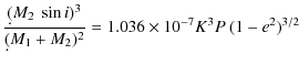$\displaystyle \frac{\d (M_2~\sin{i})^3}{\d (M_1+M_2)^2} = 1.036 \times 10^{-7} K^3 P~(1-e^2)^{3/2}$
$\displaystyle a\sin{i}$	=	$\displaystyle 9.192\times 10^{-5} K~P~(1-e^2)^{1/2}$	(2)

where K is in km s^-1, P in d, and a in AU. The large errors of the obtained mass functions of 30% for the C-C1 orbit and 60% for the C-C2 orbit mainly result from the insufficient accuracy in determining the eccentricities and K-values of the orbits.

In the following we assume that the components C, C1, and C2 of ${\it\Theta }^{\rm 1}$ Ori C build a hierarchical system where the components C and C1 of the close system orbit around their center of mass and that this center, representing the total mass of C1 plus C2, orbits with C2 around the center of mass of the wide system.

6.1 The distant companion C2

Kraus et al. (2009) determined a dynamical mass of the ${\it\Theta }^{\rm 1}$ Ori C system of (44 $\pm$ 7) $M_{\hbox{$\odot$ }}$ . By combining this, the known inclination of the C-C2 orbit (Table 10), and the spectroscopic mass function of C2 (Table 8), we can derive the mass of C2 to ( $12\pm 3$ ) $M_{\hbox{$\odot$ }}$ . I follows that he mass of C+C1 is ( $32\pm 3$ ) $M_{\hbox{$\odot$ }}$ and the mass ratio between C2 and C+C1 is $0.41\pm 0.12$ . The latter value agrees with the value of $0.45 \pm 0.15$ derived by Kraus et al. (2007) by modeling the wavelength-dependent binary flux ratio of the ${\it\Theta }^{\rm 1}$ Ori C system, whereas Kraus et al. (2009) determine $q =0.23\pm0.05$ by analyzing the RVs from Stahl et al. without applying any cleaning for additional components.

Kraus et al. (2009) estimate a dynamical distance of ${\it\Theta }^{\rm 1}$ Ori C of ( $410\pm 20$ ) pc, in agreement with the value of 414 pc given by Menten et al. (2007). From this distance and a=44 mas (Table 10), the semi-major axis of the relative orbit follows to 18 AU. The spectroscopically derived value of the semi-major axis of the orbit of the primary is of 5 AU (Table 8). The deduced mass ratio of 0.45 gives a semi-major axis of the relative orbit of a=17 AU, in good agreement with the astrometric value.

6.2 The close companion C1

From the mass function of C1 of $(10\pm 3)\times 10^{-4}$ (Table 8) and the mass of C+C1 of ( $44 \pm 7$ ) $M_{\hbox{$\odot$ }}$ we obtain a projected mass (or lower limit) of C1 of ( $1.01\pm0.16$ ) $M_{\hbox{$\odot$ }}$ so that an upper limit of (31 $\pm$ 3) $M_{\hbox{$\odot$ }}$ follows for the mass of the primary. This gives a mass ratio of $0.033 \pm0.008$ . With this mass ratio and the projected semi-major axis of the primary of ( $0.026 \pm 0.002$ ) AU (Table 8), the projected semi-major axis of the relative orbit follows to ( $0.82 \pm0.26$ ) AU.

The projected values are very close to the absolute values if we assume that the C1 and C2 orbits are coplanar ( $i_{C-C2}=99^\circ$ ). In this case the close companion would be a solar mass star revolving around the primary in a highly eccentric orbit, and the smallest distance between the components during periastron passage would be ( $0.4 \pm 0.1$ ) AU.

6.3 The rotational period of the primary

Our model assumes that the period of 61 $.\!\!^{\rm d}$ 5 d and its first two harmonics found from the multiple frequency search stand for the orbit of a close companion, where the 61 $.\!\!^{\rm d}$ 5 d period is the orbital period and the harmonics count for the deviations of the RV curve from a sinusoid due to the non-circularity of the orbit. We further assumed that the third harmonic with a period of 15 $.\!\!^{\rm d}$ 4 is the rotational period because its contribution does not vanish after cleaning the RVs for the derived orbit. A period of 15 $.\!\!^{\rm d}$ 4 was found in the RVs also by Stahl et al. (2008) and assigned to the rotation of the star. Simon-Diaz et al. (2006) derived the $v\sin{i}$ of the primary from the Fourier method to (24 $\pm$ 3) km s^-1 whereas the measurement of the FWHM of the spectral lines gave higher values by a factor of up to 2. Assuming that the 15 $.\!\!^{\rm d}$ 4 period is the rotation period and the radius of the primary is 11 $R_{\hbox{$\odot$ }}$ , the authors derived an upper limit for $v\sin{i}$ of 35 km s^-1 and an inclination of the rotation axis of (44 $\pm$ 12) $^\circ$ based on the value of $v\sin{i}$ measured by the Fourier method.

Assuming that the rotation axis of the primary is aligned with the orientation of the wide orbit ( $i=99^\circ$ ), $P_{\rm rot}$ = 15 $.\!\!^{\rm d}$ 417, and R = 11 $R_{\hbox{$\odot$ }}$ , we get $v\sin{i}$ = 36 km s^-1, a value that corresponds to the order of values obtained by Simon-Diaz et al. (2006) from the FWHM method. On the other hand, if we reject the hypothesis that the found 61 $.\!\!^{\rm d}$ 5 period and its harmonics arise from RV variations caused by orbital motion because of the unlikely high eccentricity, we have to ask for some physical process that acts on this time scale. In that case, the 61 $.\!\!^{\rm d}$ 5 period and all its observed harmonics have to be assigned to the same process - the 15 $.\!\!^{\rm d}$ 4 period cannot be the rotation period anymore.

A nearby assumption would be that the 61 $.\!\!^{\rm d}$ 5 period itself is the rotation period and its harmonics describe surface or near-to-surface inhomogeneities. In that case, however, the $v\sin{i}$ should be smaller than 9 km s^-1 for R = 11 $R_{\hbox{$\odot$ }}$ or, in case of $v\sin{i}$ = 24 km s^-1, the radius of the primary should be larger than 29 $R_{\hbox{$\odot$ }}$ . Neither is compatible with the observations.

7 Conclusions

By combining new RV measurements of ${\it\Theta }^{\rm 1}$ Ori C with data from the literature, we deduced two fundamental periods of 11 yr and 61 $.\!\!^{\rm d}$ 49. The first one is the period of the wide orbit with the known astrometric companion. The second one occurs with significant contributions from its first and third harmonics. By cleaning the RVs for the shorter fundamental period and its harmonics, we were able to derive an improved orbital solution for the wide orbit that can reproduce the observed astrometric positions. By combining the astrometric and spectroscopic findings, we derived the absolute masses of the primary of (32 $\pm$ 3) $M_{\hbox{$\odot$ }}$ and of its companion of (12 $\pm$ 3) $M_{\hbox{$\odot$ }}$ , corresponding to a mass ratio of 0.41 $\pm$ 0.12. This mass ratio is significantly greater than estimated by Kraus et al. (2009) from the uncleaned RVs measured by Stahl et al. (2008) but agrees well with the value of 0.45 $\pm$ 0.15 derived by Kraus et al. (2007) from modeling the wavelength-dependent binary flux ratio of the ${\it\Theta }^{\rm 1}$ Ori C system. All other derived system parameters agree with the astrometric findings.

Assuming that the second period of 61 $.\!\!^{\rm d}$ 49 is the orbital period of a close companion, we end up with an eccentric orbit of e = 0.49. In this case, the third harmonic, 15 $.\!\!^{\rm d}$ 42, can be found again in the residuals after subtracting the solutions for the close and the wide orbit, and we assign it to the rotation of the primary that is in a 1:4 resonance with the orbital period. The interpretation of the 15 $.\!\!^{\rm d}$ 42 as the rotational period agrees with Stahl et al. (2008) who found this period without counting for the 61 $.\!\!^{\rm d}$ 49 period and with the $v\sin{i}$ measurements by Simon-Diaz et al. (2006).

The high eccentricity of the close orbit causes some doubt about our interpretation of the 61 $.\!\!^{\rm d}$ 49 as an orbital period because one normally expects that the tidal forces of the much more massive primary should have circularized the orbit. We therefore had a closer look at the observational data with respect to the close orbit C-C1. The analysis of separated subsets of RVs showed that the period of 61 $.\!\!^{\rm d}$ 49 can be found in each of them and that the data are compatible with the derived orbital solution in each epoch of observation. On the other hand, this analysis was hampered by the fact that in most of the subsets the number of data points and its distribution in time were not sufficient to come to a precise conclusion about the behavior of the scatter of the RVs around the orbital solution. It seems, however, that this scatter is more or less evenly distributed over all epochs of observation. In the residuals there remains a trend of increasing $\gamma$ velocity with time. We tried to explain it by a decrease in the period of the C-C1 orbit but could not get significant results.

Presently, we cannot definitely say if the interpretation of the 61 $.\!\!^{\rm d}$ 49 period as an orbital period is correct. Either the close companion exists and the RVs are distorted by photospheric or magnetospheric activity or we observe the effects of such activity on different time scales with some underlying quasi-periodicity with a typical time scale of 61 $.\!\!^{\rm d}$ 49. In the latter case, the existence of the 15 $.\!\!^{\rm d}$ 42 period can hardly be explained as the rotational period, it will be simply an overtone of the basic time scale of 61 $.\!\!^{\rm d}$ 49. We can exclude 61 $.\!\!^{\rm d}$ 49 as the rotational period because it is not compatible with the $v\sin{i}$ as measured by Simon-Diaz et al. (2006). However, there are a lot of findings that favor the 15 $.\!\!^{\rm d}$ 42 period as the rotational period. It is compatible with the measured $v\sin{i}$ , and with the suggested model of an oblique magnetic rotator for ${\it\Theta }^{\rm 1}$ Ori C (Stahl et al. 1996) that is also agrees with the X-ray observations. Based on observations with the ROSAT satellite, Gagne et al. (1997) came to the conclusion that the observed X-ray variability can be explained either by an absorption of magnetospheric X-rays in a corotating wind or by magnetosphere eclipses. Both explanations assume a very extended magnetosphere of the star and are based on the 15 $.\!\!^{\rm d}$ 42 period.

Assuming that our model of a triple star is valid and that the close and wide orbits are coplanar, we end up with absolute masses of the primary of (31 $\pm$ 3) $M_{\hbox{$\odot$ }}$ and of the close companion of (1.01 $\pm$ 0.16) $M_{\hbox{$\odot$ }}$ . The semi-major axis of the close orbit is of (0.82 $\pm$ 0.26) AU.

Although the scatter in the residuals of the orbital solution could be reduced by cleaning the RVs for the 61 $.\!\!^{\rm d}$ 49 period and, independent of its nature, for its harmonics, the remaining scatter exceeds the estimated errors of measurement. An apsidal advance of the close orbit due to the tidal interaction with the distant companion could be excluded as the main reason for this scatter. On the other hand, its detection could help to confirm the assumed structure of a triple system. The still too short time base of our observations and the RV variations of ${\it\Theta }^{\rm 1}$ Ori C caused by additional processes prevent us from a certain statement, however.

The Nyquist frequency of the time sampling of our data is about 0.5 c d^-1. Up to this frequency, we can exclude additional RV variations due to strongly periodic processes. We assume that the remaining scatter in the residuals comes from quasi-periodic as well as from irregular variations on different time scales. We do not want to speculate about the underlying processes based on our observations in the visual range but refer to the model by Babel & Montmerle (1997) derived from the X-ray variability and to the wide range of effects that can be expected from the interaction of the large-scale, oblique, magnetic field with the stellar wind.

The star ${\it\Theta }^{\rm 1}$ Ori C has been studied for about 90 years and about a hundred of papers have been dedicated to it. However, lines of the satellites could not be detected in its spectrum until now. It seems that there is no chance to detect the lines of the assumed close companion. The light contribution of a one solar mass star compared to that of the 30 times more massive primary should be negligible, at least in the visual range. Although we have so far not found any contribution from the distant companion in the spectra of ${\it\Theta }^{\rm 1}$ Ori C, the V-band flux ratio of 0.32 deduced by Kraus et al. (2007) let us hope to find such lines in the future, based on the actual findings and by applying more advanced methods of spectral decomposing like KOREL (Hadrava 1995,2006).

Acknowledgements

We are grateful to V. Tsymbal and I. Bikmaev for useful discussions and to J. Lancaster, E. Brevnova, A. Serber, N. Bondar, and Z. Scherbakova, who supported us in preparing this paper. We want to thank the referee, O. Stahl, for his useful comments that helped us to improve the article.

References

Babel, J., & Montmerle, Th. 1997, ApJ 485, L29 [Google Scholar]
Conti, P. S. 1972, ApJ, 174, L79 [NASA ADS] [CrossRef] [Google Scholar]
Donati, F., Babel, J., Harries, T. J., & et al. 2002, MNRAS 333, 55 [NASA ADS] [CrossRef] [MathSciNet] [Google Scholar]
Folker, J. 1994, Proc. Fourth European IUE conf., esa SP-218 [Google Scholar]
Frost, E. B., Barret, S. B., & Struve, O. 1926, ApJ, 64, 1 [NASA ADS] [CrossRef] [Google Scholar]
Gagne, M., Caillault, J.-P., Stauffer, J., et al. 1997, ApJ, 478, L87 [NASA ADS] [CrossRef] [Google Scholar]
Galazutdinov, G. A. 1992, Prepr. SAO RAS, No. 92 (www.gazinur.com) [Google Scholar]
Hadrava, P. 1995, A&AS, 114, 393 [NASA ADS] [Google Scholar]
Hadrava, P. 2006, A&A, 448, 1149 [NASA ADS] [CrossRef] [EDP Sciences] [Google Scholar]
Hartkopf, W. I., & McAlister, H. A. 1989, AJ 98, 1014 [NASA ADS] [CrossRef] [Google Scholar]
Heintz, W. D. 1978, Double Stars (Dordrecht: D. Reidel Publ. Co.) [Google Scholar]
Kraus, S., Balega, Y. Y., .Berger, J.-P., et al. 2007, A&A, 466, 649 [NASA ADS] [CrossRef] [EDP Sciences] [Google Scholar]
Kraus, S., Weigelt, G., Balega, J. J., et al. 2009, A&A, 497, 195 [NASA ADS] [CrossRef] [EDP Sciences] [Google Scholar]
Kukarkin, B., Kholopov, P. N., Artyuckina, N. M., et al. 1982, New catalogue of suspected variable stars (Moscow: Nauka) [Google Scholar]
Menten, K. M., Reid, M. J., Forbrich, J., et al. 2007, A&A, 474, 515 [NASA ADS] [CrossRef] [EDP Sciences] [Google Scholar]
Simon-Diaz, S., Herrero, A., Esteban, C., et al. 2006, A&A 448, 351 [NASA ADS] [CrossRef] [EDP Sciences] [Google Scholar]
Stahl, O., Wolf, B., Gang, Th., et al. 1993, A&A, 274, L29 [NASA ADS] [Google Scholar]
Stahl, O., Kaufer, A, Rifinis, Th., et al. 1996, A&A, 312, 539 [NASA ADS] [Google Scholar]
Stahl, O., Wade, G., Petit, V., et al. 2008, A&A, 487, 323 [NASA ADS] [CrossRef] [EDP Sciences] [Google Scholar]
Stetsenko, D. V., Bikmaev, I. F., & Vitrichenko, E. A. 2007, 271, Spectroscopic methods in modern astrophysics (Moscow: Janus-K, in Russian) [Google Scholar]
Struve, O., & Titus, J. 1944, ApJ, 99, 84 [NASA ADS] [CrossRef] [Google Scholar]
van Genderen, A. M., Bovenchen, H., Engelsman, E. C., et al. 1989, A&AS, 79, 263 [NASA ADS] [Google Scholar]
Vitrichenko, E. A. 2000, Astron. Lett., 26, 244 [NASA ADS] [CrossRef] [Google Scholar]
Vitrichenko, E. A. 2002, Astron. Lett., 28, 324 [NASA ADS] [CrossRef] [Google Scholar]
Vitrichenko, E. A. 2004, Orion Trapezium (Moscow: Nauka) [Google Scholar]
Vitrichenko, E. A. 2007, Prepr. Space Research Institute RAS No. 2139 [Google Scholar]
Walborn, N. R. 1981, ApJ, 243, L37 [NASA ADS] [CrossRef] [Google Scholar]
Walborn, N. R., & Nichols, J. S. 1994, ApJ, 425, L29 [NASA ADS] [CrossRef] [Google Scholar]
Weigelt, G., Balega, Y., Preibisch ,T., et al. 1999, A&A, 347, L15 [NASA ADS] [Google Scholar]

Footnotes

... Archive: http://atlas.obs-hp.fr/elodie/common.css
... PERIOD04: Copyright (©) 2004-2008 Patrick Lenz, Institute of Astronomy, University of Vienna

All Tables