| Issue |
A&A
Volume 513, April 2010
|
|
|---|---|---|
| Article Number | A59 | |
| Number of page(s) | 9 | |
| Section | Cosmology (including clusters of galaxies) | |
| DOI | https://doi.org/10.1051/0004-6361/200913214 | |
| Published online | 29 April 2010 | |
Probing local non-Gaussianities within a Bayesian framework
F. Elsner1 - B. D. Wandelt2,3 - M. D. Schneider4
1 - Max-Planck-Institut für Astrophysik,
Karl-Schwarzschild-Straße 1, 85748 Garching, Germany
2 -
Department of Physics, University of Illinois at
Urbana-Champaign, 1110 W. Green Street, Urbana, IL 61801, USA
3 -
Department of Astronomy, University of Illinois at
Urbana-Champaign, 1002 W. Green Street, Urbana, IL 61801, USA
4 -
Institute for Computational Cosmology, Department of Physics, Durham
University, South Road, Durham, DH1 3LE, UK
Received 31 August 2009 / Accepted 31 January 2010
Abstract
Aims. We outline the Bayesian approach to inferring
![]() ,
the level of non-Gaussianities of local type. Phrasing
,
the level of non-Gaussianities of local type. Phrasing
![]() inference in a Bayesian framework takes advantage of existing
techniques to account for instrumental effects and foreground
contamination in CMB data and takes into account uncertainties in the
cosmological parameters in an unambiguous way.
inference in a Bayesian framework takes advantage of existing
techniques to account for instrumental effects and foreground
contamination in CMB data and takes into account uncertainties in the
cosmological parameters in an unambiguous way.
Methods. We derive closed form expressions for the joint posterior of
![]() and the reconstructed underlying curvature perturbation,
and the reconstructed underlying curvature perturbation, ![]() ,
and deduce the conditional probability densities for
,
and deduce the conditional probability densities for
![]() and
and ![]() .
Completing the inference problem amounts to finding the marginal density for
.
Completing the inference problem amounts to finding the marginal density for
![]() .
For realistic data sets the necessary integrations are intractable. We
propose an exact Hamiltonian sampling algorithm to generate correlated
samples from the
.
For realistic data sets the necessary integrations are intractable. We
propose an exact Hamiltonian sampling algorithm to generate correlated
samples from the
![]() posterior. For sufficiently high signal-to-noise ratios, we can exploit
the assumption of weak non-Gaussianity to find a direct Monte Carlo
technique to generate independent samples from the posterior distribution for
posterior. For sufficiently high signal-to-noise ratios, we can exploit
the assumption of weak non-Gaussianity to find a direct Monte Carlo
technique to generate independent samples from the posterior distribution for
![]() .
We illustrate our approach using a simplified toy model of CMB data for the simple case of a 1D sky.
.
We illustrate our approach using a simplified toy model of CMB data for the simple case of a 1D sky.
Results. When applied to our toy problem, we find that, in the
limit of high signal-to-noise, the sampling efficiency of the
approximate algorithm outperforms that of Hamiltonian sampling by two
orders of magnitude. When
![]() is not significantly constrained by the data, the more efficient,
approximate algorithm biases the posterior density towards
is not significantly constrained by the data, the more efficient,
approximate algorithm biases the posterior density towards
![]() .
.
Key words: cosmic microwave background - cosmological parameters - methods: data analysis - methods: numerical - methods: statistical
1 Introduction
The analysis of cosmic microwave background (CMB) radiation data has considerably improved our understanding of cosmology and played a crucial role in constraining the set of fundamental cosmological parameters of the universe (Spergel et al. 2007; Hinshaw et al. 2009). This success is based on the intimate link between the temperature fluctuations we observe today and the physical processes taking place in the very early universe. Inflation is currently the favored theory predicting the shape of primordial perturbations (Linde 1982; Guth 1981), which in its canonical form leads to very small non-Gaussianities that are far from being detectable by means of present-day experiments (Maldacena 2003; Acquaviva et al. 2003). However, inflation scenarios producing larger amounts of non-Gaussianity can naturally be constructed by breaking one or more of the following properties of canonical inflation: slow-roll, single-field, Bunch-Davies vacuum, or a canonical kinetic term (Bartolo et al. 2004). Thus, a positive detection of primordial non-Gaussianity would allow us to rule out the simplest models. Combined with improving constraints on the scalar spectral index ns, the test for non-Gaussianity is therefore complementary to the search for gravitational waves as a means to test the physics of the early Universe.
A common strategy for estimating primordial non-Gaussianity is to examine a cubic combination of filtered CMB sky maps (Komatsu et al. 2005). This approach takes advantage of the specific bispectrum signatures produced by primordial non-Gaussianity and yields to a computationally efficient algorithm. When combined with the variance reduction technique first described by Creminelli et al. (2006) these bispectrum-based techniques are close to optimal, where optimality is defined as saturation of the Cramer-Rao bound. Lately, a more computationally costly minimum variance estimator has been implemented and applied to the WMAP5 data (Smith et al. 2009).
Recently, a Bayesian approach has been introduced in CMB power spectrum analysis and applied successfully to WMAP data making use of Gibbs-sampling techniques (Jewell et al. 2004; Wandelt et al. 2004). Within this framework, one draws samples from the posterior probability density given by the data without explicitly calculating it. The target probability distribution is finally constructed out of the samples directly, thus computationally costly evaluations of the likelihood function or its derivatives are not necessary. Another advantage of the Bayesian analysis is that the method naturally offers the possibility to include a consistent treatment of the uncertainties associated with foreground emission or instrumental effects (Eriksen et al. 2008). As it is possible to model CMB and foregrounds jointly, statistical interdependencies can be directly factored into the calculations. This is not straightforward in the frequentist approach where the data analysis is usually performed in consecutive steps. Yet another important and desirable feature is the fact that a Bayesian analysis obviates the necessity to specify fiducial parameters, whereas in the frequentist approach it is only possible to test one individual null hypothesis at a time.
In this paper, we pursue the modest goal of developing the formalism for the extension of the Bayesian approach to the analysis of non-Gaussian signals, in particular to local models, where the primordial perturbations can be modeled as a spatially local, non-linear transformation of a Gaussian random field. Utilizing this method, we are able to write down the full posterior probability density function (PDF) of the level of non-Gaussianity. We demonstrate the principal aspects of our approach using a 1D toy sky model. Although we draw our discussion on the example of CMB data analysis, the formalism presented here is of general validity and may also be applied within a different context.
The paper is organized as follows. In Sect. 2 we give a short overview of the theoretical background used to characterize primordial perturbations. We present a new approximative approach to extract the amplitude of non-Gaussianities from a map in Sect. 3 and verify the method by means of a simple synthetic data model (Sect. 4). After addressing the question of optimality in Sect. 5, we compare the performance of our technique to an exact Hamiltonian Monte Carlo sampler which we develop in Sect. 6 and discuss the extensions of the model required to deal with a realistic CMB sky map (Sect. 7). Finally, we summarize our results in Sect. 8.
2 Model of non-Gaussianity
The expansion coefficients
![]() of the observed CMB
temperature anisotropies in harmonic space can be related to the
primordial fluctuations via
of the observed CMB
temperature anisotropies in harmonic space can be related to the
primordial fluctuations via
where
Any non-Gaussian signature imprinted in the primordial perturbations will be
transferred to the
![]() according to Eq. (1) and is
therefore detectable, in principle. Theoretical models predicting
significant levels of non-Gaussian contributions to the observed signal can
be subdivided into two broad classes (Babich et al. 2004): one
producing non-Gaussianity of local type, the other of equilateral
type. The former kind of non-Gaussianity is achieved to very good approximation
in multi-field inflation as described by the curvaton model
(Enqvist & Sloth 2002; Moroi & Takahashi 2001; Lyth et al. 2003), or in
cyclic/ekpyrotic universe models (Steinhardt & Turok 2002; Khoury et al. 2001). The latter type of non-Gaussianity is typically a result
of single field models with non-minimal Lagrangian including higher
order derivatives (Senatore 2005; Alishahiha et al. 2004).
according to Eq. (1) and is
therefore detectable, in principle. Theoretical models predicting
significant levels of non-Gaussian contributions to the observed signal can
be subdivided into two broad classes (Babich et al. 2004): one
producing non-Gaussianity of local type, the other of equilateral
type. The former kind of non-Gaussianity is achieved to very good approximation
in multi-field inflation as described by the curvaton model
(Enqvist & Sloth 2002; Moroi & Takahashi 2001; Lyth et al. 2003), or in
cyclic/ekpyrotic universe models (Steinhardt & Turok 2002; Khoury et al. 2001). The latter type of non-Gaussianity is typically a result
of single field models with non-minimal Lagrangian including higher
order derivatives (Senatore 2005; Alishahiha et al. 2004).
Concentrating on local models, we can parametrize the non-Gaussianity of ![]() by introducing an additional quadratic dependence on a purely
Gaussian auxiliary field
by introducing an additional quadratic dependence on a purely
Gaussian auxiliary field
![]() ,
that is local in real space, of the
form (Verde et al. 2000; Komatsu & Spergel 2001)
,
that is local in real space, of the
form (Verde et al. 2000; Komatsu & Spergel 2001)
where
3 Bayesian inference of non-Gaussianity
It has been shown to be feasible to reconstruct the primordial
curvature potential out of temperature or temperature and polarization
sky maps (Yadav & Wandelt 2005; Elsner & Wandelt 2009), which allows
searching for primordial non-Gaussianities more sensitively. Although the mapping
from a 3D potential to a 2D CMB sky map is not invertible
unambiguously, a unique solution can be found by requiring that the
result minimizes the variance. In this conventional frequentist
approach, the level of non-Gaussianity and an estimate of its error is derived
from a cubic combination of filtered sky maps
(Komatsu et al. 2005). We will show in the following sections
how to sample
![]() from the data and unveil the full posterior PDF
using a Bayesian approach.
from the data and unveil the full posterior PDF
using a Bayesian approach.
3.1 Joint probability distribution
In our analysis we assume the data vector d to be a superposition of
the CMB signal s and additive noise n
| d | = | B s + n | |
| = | (3) |
where information about observing strategy and the optical system are encoded in a pointing matrix B and M is a linear transformation matrix. In harmonic space, the signal is related to the primordial scalar perturbation as
| |
= | ||
| (4) |
Our aim is to construct the posterior PDF of the amplitude of non-Gaussianities given by the data,
| (5) |
Now, we can use Eq. (2) to express the probability for data dgiven
| (6) |
where N is the noise covariance matrix. The prior probability
distribution for
![]() given
given ![]() can be expressed by a
multivariate Gaussian by definition. Using the covariance matrix
can be expressed by a
multivariate Gaussian by definition. Using the covariance matrix ![]() of the potential, we derive
of the potential, we derive
For flat priors
![$\displaystyle %
\left.\qquad \times \big(d - B M \big( \Phi_{{{\rm L}}} + f_{{{...
...^{\dagger}
P^{-1}_{\Phi} \Phi_{{{\rm L}}} \big] \vphantom{\frac{1}{2}} \right\}$](/articles/aa/full_html/2010/05/aa13214-09/img42.png)
![]() as an exact expression for the joint distribution up to a
normalization factor.
as an exact expression for the joint distribution up to a
normalization factor.
To derive the posterior density,
![]() ,
one has to
marginalize the joint distribution over
,
one has to
marginalize the joint distribution over
![]() and
and ![]() .
As
it is not possible to calculate the high dimensional
.
As
it is not possible to calculate the high dimensional
![]() integral directly, an effective sampling scheme must be found to
evaluate the expression by means of a Monte Carlo algorithm. One
possibility would be to let a Gibbs sampler explore the parameter
space. Unfortunately, we were not able to find an efficient sampling
recipe from the conditional densities for
integral directly, an effective sampling scheme must be found to
evaluate the expression by means of a Monte Carlo algorithm. One
possibility would be to let a Gibbs sampler explore the parameter
space. Unfortunately, we were not able to find an efficient sampling
recipe from the conditional densities for
![]() and
and
![]() as
the variables are highly correlated. An algorithm that also generates
correlated samples, but is potentially suitable for non-Gaussian densities
and high degrees of correlation is the Hamiltonian Monte Carlo
approach. We will return to this approach in Sect. 6.
as
the variables are highly correlated. An algorithm that also generates
correlated samples, but is potentially suitable for non-Gaussian densities
and high degrees of correlation is the Hamiltonian Monte Carlo
approach. We will return to this approach in Sect. 6.
For now we attempt to go beyond correlated samplers and see whether we
can develop an approximate scheme, valid in the limit of weak non-Gaussianity, to
sample
![]() independently. We start out by expanding the target
posterior distribution into an integral of conditional probabilities
over the non-linear potential
independently. We start out by expanding the target
posterior distribution into an integral of conditional probabilities
over the non-linear potential
![]() ,
,
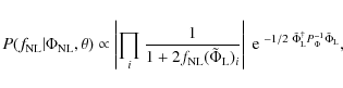
To construct the conditional probability
| |
= | ||
| = | |||
| = | (10) |
As the covariance matrix
Note, that the approximation applies to the second term only, the first part of the expression remains unaffected. As this approximation is equivalent to imposing the prior belief of purely Gaussian primordial perturbations, we expect to underestimate
The direct evaluation of the joint distributions over a grid in the high dimensional parameter space is computationally not feasible. One option would be to approximate the PDF around its maximum to get an expression for the attributed errors (Tegmark 1997; Bond et al. 1998). These methods are still computationally expensive and can also not recover the full posterior. An alternative approach to overcome these problems is to draw samples from the PDF which is to be evaluated as we will discuss in the next section.
3.2 Conditional probabilities
To construct the target posterior density Eq. (9), we have to find expressions for the conditional probabilities
![$\displaystyle \langle (\Phi_{{{\rm NL}}} - \langle \Phi_{{{\rm NL}}} \rangle )^2 \rangle = \left[
M^{\dagger} B^{\dagger} N^{-1} B M + P_\Phi^{-1} \right]^{-1} .$](/articles/aa/full_html/2010/05/aa13214-09/img57.png)
As a next step, we derive the conditional probability distribution of
![]() for given
for given
![]() .
This expression is not affected by the
approximation and can be derived from a marginalization over
.
This expression is not affected by the
approximation and can be derived from a marginalization over
![]() ,
,
| (13) |
Using Eq. (7), we can calculate the integral and obtain
where
![]() is a function of
is a function of
![]() and can be regarded
as inversion of Eq. (2),
and can be regarded
as inversion of Eq. (2),
![\begin{displaymath}
\tilde{\Phi}_{{{\rm L}}} = \frac{1}{2 f_{{{\rm NL}}}} \left[...
...left\langle \Phi^2_{{{\rm L}}} \right\rangle\right)} \right] .
\end{displaymath}](/articles/aa/full_html/2010/05/aa13214-09/img62.png)
Note that we can resolve the ambiguity in sign in the weakly non-Gaussian limit (Babich 2005). Because the absolute value of the
elements of the second solution is typically larger by orders of
magnitude, the probability of its realization is strongly disfavored
by the prior
![]() .
The factor of suppression is typically
less than
10-1000 and further vanishing with decreasing
.
The factor of suppression is typically
less than
10-1000 and further vanishing with decreasing
![]() .
.
After setting up the conditional densities, we now can sample from the
distributions iteratively. First, we draw
![]() from a Gaussian distribution using Eqs. (12). Then,
from a Gaussian distribution using Eqs. (12). Then,
![]() can be sampled
according to Eq. (14) using the value of
can be sampled
according to Eq. (14) using the value of
![]() derived
in the preceding step. Thus, the sampling scheme reads as
derived
in the preceding step. Thus, the sampling scheme reads as
Note that this is not Gibbs sampling. For a fixed set of
cosmological parameters, we can chain together samples from the
conditional densities above, producing independent
![]() samples. The efficiency of such a direct Monte Carlo sampler is
therefore expected to be much higher than that of a Gibbs sampler,
which, in the general case, would produce correlated samples.
samples. The efficiency of such a direct Monte Carlo sampler is
therefore expected to be much higher than that of a Gibbs sampler,
which, in the general case, would produce correlated samples.
As an extension of the sampling scheme presented so far, we sketch an
approach to account for uncertainties in cosmological parameters and
foreground contributions. Complementing the scheme (Eqs. (16))
by an additional step allows to take into account the error in the
parameters ![]() ,
,
| (17) |
where the last equation updates the cosmological parameters that can
be sampled from the data by means of standard Monte Carlo analysis
tools![]() . Now, the scheme formally reads as a
Gibbs sampler and can in principle take into account the correlation
among
. Now, the scheme formally reads as a
Gibbs sampler and can in principle take into account the correlation
among
![]() and the other cosmological parameters exactly. In
practice, however, the impact of a non-vanishing
and the other cosmological parameters exactly. In
practice, however, the impact of a non-vanishing
![]() is expected to
be negligible, i.e.
is expected to
be negligible, i.e.
![]() .
Likewise, we can allow for an additional sampling step to deal
with foreground contributions, e.g. from synchrotron, free-free, and
dust emission. Foreground templates
.
Likewise, we can allow for an additional sampling step to deal
with foreground contributions, e.g. from synchrotron, free-free, and
dust emission. Foreground templates
![]() ,
that
are available for these sources, can be subtracted with amplitudes
,
that
are available for these sources, can be subtracted with amplitudes
![]() which are sampled from the data in each
iteration,
which are sampled from the data in each
iteration,
![]() (Wandelt et al. 2004). Alternatively, component
separation techniques could be used to take foreground contaminants
into account without the need to rely on a priori defined templates
(Eriksen et al. 2006). The traditional approach to deal with
point sources is to mask affected regions of the sky to exclude them
from the analysis. Discrete object detection has been demonstrated to
be possible within a Bayesian framework (Carvalho et al. 2009; Hobson & McLachlan 2003), and can be fully included into the sampling
chain. However, as sources are only successfully detected down to an
experiment-specific flux limit, a residue-free removal of their
contribution is in general not possible.
(Wandelt et al. 2004). Alternatively, component
separation techniques could be used to take foreground contaminants
into account without the need to rely on a priori defined templates
(Eriksen et al. 2006). The traditional approach to deal with
point sources is to mask affected regions of the sky to exclude them
from the analysis. Discrete object detection has been demonstrated to
be possible within a Bayesian framework (Carvalho et al. 2009; Hobson & McLachlan 2003), and can be fully included into the sampling
chain. However, as sources are only successfully detected down to an
experiment-specific flux limit, a residue-free removal of their
contribution is in general not possible.
|
Figure 1:
Examples of reconstructed potentials
|
| Open with DEXTER | |
|
Figure 2:
Examples of a constructed posterior distribution for
|
| Open with DEXTER | |
|
Figure 3:
Build-up of the posterior distribution of
|
| Open with DEXTER | |
As the angular resolution of sky maps produced by existing CMB
experiments like WMAP is high and will further increase once data of
the Planck satellite mission becomes available, computational
feasibility of an analysis tool is an issue. The speed of our method
in a full implementation is limited by harmonic transforms which scale
as
![]() and are needed to calculate the
primordial perturbations at numerous shells at distances from the
cosmic horizon to zero. Thus, it shows the same scaling relation as
fast cubic estimators (Komatsu et al. 2005; Yadav et al. 2007), albeit with a larger prefactor.
and are needed to calculate the
primordial perturbations at numerous shells at distances from the
cosmic horizon to zero. Thus, it shows the same scaling relation as
fast cubic estimators (Komatsu et al. 2005; Yadav et al. 2007), albeit with a larger prefactor.
|
Figure 4:
Properties of the sampler. Left panel: shown is the
distribution of the derived mean values of
|
| Open with DEXTER | |
| Figure 5:
Impact of the signal-to-noise ratio on the approximate sampling
scheme. Left panel: example of a constructed posterior
distribution for S/N = 10. Middle panel: analysis of the
same data set, but for S/N = 0.5. At high noise level, the
distribution becomes too narrow and systematically shifted towards
|
|
| Open with DEXTER | |
4 Implementation and discussion
To verify our results and demonstrate the applicability of the method, we implemented a simple 1D toy model. We considered a vector
|
(18) |
Then, a data vector with weak non-Gaussianity according to Eq. (2) was produced and superimposed with Gaussian white noise. Constructed in this way, it is of the order
The data vector had a length of 106 pixels; for simplicity, we set the beam function B and the linear transformation matrix M to unity. This setup allows a brute force implementation of all equations at a sufficient computational speed. We define the signal-to-noise ratio (S/N) per pixel as the standard deviation of the input signal divided by the standard deviation of the additive noise. It was chosen in the range 0.5-10 to model the typical S/N per pixel of most CMB experiments. To reconstruct the signal, we draw 1000 samples according to the scheme in Eq. (16).
Whereas the
![]() can be generated directly from a simple Gaussian distribution with known mean and variance, the construction of the
can be generated directly from a simple Gaussian distribution with known mean and variance, the construction of the
![]() is slightly more complex. For each
is slightly more complex. For each
![]() ,
we ran a
Metropolis Hastings algorithm with symmetric Gaussian proposal density
with a width comparable to that of the target density and started the
chain at
,
we ran a
Metropolis Hastings algorithm with symmetric Gaussian proposal density
with a width comparable to that of the target density and started the
chain at
![]() .
We run the
.
We run the
![]() chain to convergence. We
ensured that after ten accepted steps the sampler has decorrelated
from the starting point. Our tests conducted with several chains run
in parallel give
1 < R < 1.01, where R is the convergence statistic
proposed by Gelman & Rubin (1992). We record the last element of the chain as
the new
chain to convergence. We
ensured that after ten accepted steps the sampler has decorrelated
from the starting point. Our tests conducted with several chains run
in parallel give
1 < R < 1.01, where R is the convergence statistic
proposed by Gelman & Rubin (1992). We record the last element of the chain as
the new
![]() sample.
sample.
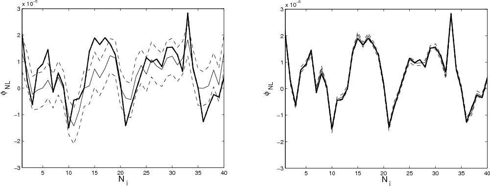
Finally, we compared the obtained sets of values
![]() ,
,
![]() to the initial data. An example is shown in
Fig. 1, where we illustrate the reconstruction of a given
potential
to the initial data. An example is shown in
Fig. 1, where we illustrate the reconstruction of a given
potential
![]() for different signal-to-noise ratios per
pixel. The
for different signal-to-noise ratios per
pixel. The ![]() error bounds are calculated from the 16% and 84% quantile of the generated sample. Typical posterior densities
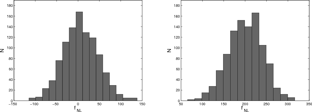
for
error bounds are calculated from the 16% and 84% quantile of the generated sample. Typical posterior densities
for
![]() as derived from the samples can be seen in
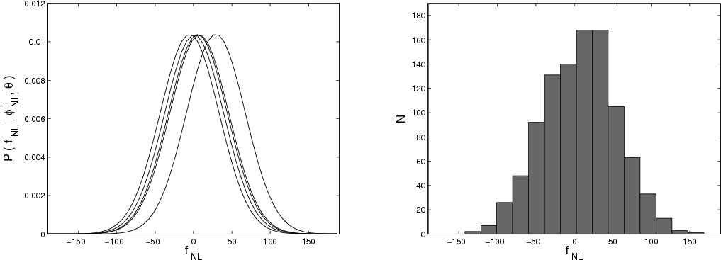
Fig. 2. We considered the cases
as derived from the samples can be seen in
Fig. 2. We considered the cases
![]() and
and
![]() with S/N = 10 per pixel and show the distributions
generated from 1000 draws. The derived posterior densities possesses
a mean value of
with S/N = 10 per pixel and show the distributions
generated from 1000 draws. The derived posterior densities possesses
a mean value of
![]() and
and
![]() ,
respectively. The width of the posterior is determined by both the
shape of the conditional PDF of
,
respectively. The width of the posterior is determined by both the
shape of the conditional PDF of
![]() for a given
for a given
![]() and the
shift of this distribution for different draws of
and the
shift of this distribution for different draws of
![]() (Fig. 3). The analysis of several data sets indicate that
the approximation does not bias the posterior density if the data are
decisive. We illustrate this issue in the left panel of
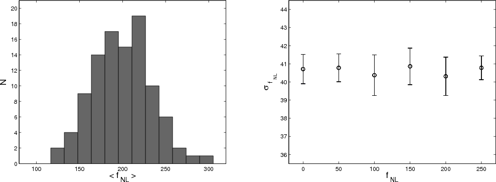
Fig. 4, where we show the distribution of the mean
values
(Fig. 3). The analysis of several data sets indicate that
the approximation does not bias the posterior density if the data are
decisive. We illustrate this issue in the left panel of
Fig. 4, where we show the distribution of the mean
values
![]() of the posterior density constructed
from 100 independent simulations. For an input value of
of the posterior density constructed
from 100 independent simulations. For an input value of
![]() we derive a mean value
we derive a mean value
![]() and conclude that our sampler is unbiased for these input
parameters. For a high noise level, however, the
and conclude that our sampler is unbiased for these input
parameters. For a high noise level, however, the
![]() can
always be sampled such that they are purely Gaussian fields and thus the
resulting PDF for
can
always be sampled such that they are purely Gaussian fields and thus the
resulting PDF for
![]() is then shifted towards
is then shifted towards
![]() .
This
behavior is demonstrated in Fig. 5 where we compare the
constructed posterior density for the cases S/N = 10 and S/N = 0.5per pixel. If the noise level becomes high, the approximated prior
distribution dominates and leads to both, a systematic displacement
and an artificially reduced width of the posterior. Therefore, the
sampler constructed here is conservative in a sense that it will tend
to underpredict the value of
.
This
behavior is demonstrated in Fig. 5 where we compare the
constructed posterior density for the cases S/N = 10 and S/N = 0.5per pixel. If the noise level becomes high, the approximated prior
distribution dominates and leads to both, a systematic displacement
and an artificially reduced width of the posterior. Therefore, the
sampler constructed here is conservative in a sense that it will tend
to underpredict the value of
![]() if the data are ambiguous.
if the data are ambiguous.
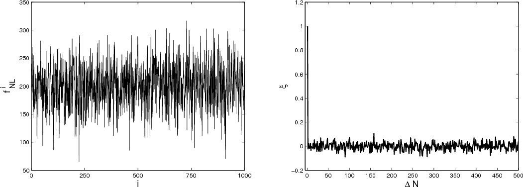
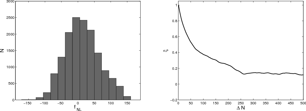
An example of the evolution of the drawn
![]() samples with time can
be seen in Fig. 6, where we in addition show the
corresponding autocorrelation function as defined via
samples with time can
be seen in Fig. 6, where we in addition show the
corresponding autocorrelation function as defined via
|
(19) |
where N is the length of the generated
5 Optimality
In a frequentist analysis, parameter inference corresponds to finding
an estimator that enables to compute the most probable value of the
quantity of interest as well as a bound for the error. Ideally, the
estimator is unbiased and optimal, i.e. it's expectation value
coincides with the true value of the parameter and the error satisfies
the Cramer-Rao bound. Contrary, in a Bayesian approach, one
calculates the full probability distribution of the parameter
directly. Strictly speaking, optimality is therefore an ill-defined
term within the Bayesian framework. All we have to show is that the
approximation adopted in Eq. (11) does not affect the
outcome of the calculation significantly. Note that the simplification
corresponds to imposing the prior of a purely Gaussian data set. In the
case of the CMB, this is a very reasonable assumption because up to
now no detection of
![]() has been reported.
has been reported.
To investigate the effects of the approximation, we checked the
dependence of the width of the posterior distribution on
![]() by
running a set of simulations with varying input values
by
running a set of simulations with varying input values
![]() ,
50, 100, 150, 200, 250. The estimated standard deviation
,
50, 100, 150, 200, 250. The estimated standard deviation
![]() of the drawn
of the drawn
![]() samples, each averaged over 10 simulation runs, are depicted in the right panel of
Fig. 4. Contrary to the KSW estimator that shows an
increase of
samples, each averaged over 10 simulation runs, are depicted in the right panel of
Fig. 4. Contrary to the KSW estimator that shows an
increase of
![]() with
with
![]() ,
we find no such indication
of sub-optimal behavior in the relevant region of small non-Gaussianity. In
particular, as the width of the distribution stays constant in the
limit
,
we find no such indication
of sub-optimal behavior in the relevant region of small non-Gaussianity. In
particular, as the width of the distribution stays constant in the
limit
![]() where our approximated equations evolve
into the exact expressions, we conclude that the adopted
simplification does not affect the result significantly.
where our approximated equations evolve
into the exact expressions, we conclude that the adopted
simplification does not affect the result significantly.
This finding can also be interpreted from a different point of view:
It is possible to define a frequentist estimator for
![]() based on
the mean of the posterior distribution. Our results indicate that such
an estimator is unbiased in the high signal-to-noise regime.
based on
the mean of the posterior distribution. Our results indicate that such
an estimator is unbiased in the high signal-to-noise regime.
We apply an additional test in the next section where we compare our sampling algorithm to a slower but exact scheme.
|
Figure 6:
Example
|
| Open with DEXTER | |
6 Hamiltonian Monte Carlo sampling
In addition to the sampling technique presented above, we tested
whether an exact Hamiltonian Monte Carlo (HMC) sampler is applicable
to the problem. Within this approach one uses the methods developed in
classical mechanics to describe the motion of particles in
potentials. The quantity of interest is regarded as the spatial
coordinate of a particle and the potential well corresponds to the PDF
to evaluate (Duane et al. 1987). To each variable
![]() ,
a mass and a momentum is
assigned and the system is evolved deterministically from a starting
point according to the Hamilton equations of motion.
,
a mass and a momentum is
assigned and the system is evolved deterministically from a starting
point according to the Hamilton equations of motion.
The applicability of HMC sampling techniques to cosmological parameter
estimation has been demonstrated in Hajian (2007), and
the authors of Taylor et al. (2008) compared HMC with Gibbs
sampling for CMB power spectrum analysis. To apply HMC sampling to
![]() inference, we deduced the expression of the Hamiltonian
inference, we deduced the expression of the Hamiltonian
![\begin{displaymath}H = \sum_{i} \frac{p^2_{i}}{2 ~ m_{i}} - \log[
P(d,\Phi_{{{\rm L}}},f_{{{\rm NL}}},\theta) ] ,
\end{displaymath}](/articles/aa/full_html/2010/05/aa13214-09/img93.png)
|
(20) |
where the potential is related to the PDF as defined in Eq. (8). The Hamilton equations of motion,

|
|||
![$\displaystyle \frac{{{\rm d}}p_{i}}{{\rm d}t} =
-\frac{\partial H}{\partial {x_...
...\partial
\log[P(d,\Phi_{{{\rm L}}},f_{{{\rm NL}}},\theta)]}{\partial {x_{i}}} ,$](/articles/aa/full_html/2010/05/aa13214-09/img95.png)
|
(21) |
are integrated for each parameter
![$\displaystyle p_{i}\left(t + \frac{\delta t}{2}\right) = p_{i}(t) + \frac{\delt...
...(d,\Phi_{{{\rm L}}},f_{{{\rm NL}}},\theta)]}{\partial x_{i}}
\bigg\vert _{x(t)}$](/articles/aa/full_html/2010/05/aa13214-09/img98.png)
|
|||
![$\displaystyle p_{i}(t + \delta t) = p_{i}\left(t + \frac{\delta t}{2}\right) + ...
...},f_{{{\rm NL}}},\theta)]}{\partial {x_{i}}}\bigg\vert _{x(t
+ \delta t)} \cdot$](/articles/aa/full_html/2010/05/aa13214-09/img100.png)
|
(22) |
The equations of motion for xi are straightforward to compute, as they only depend on the momentum variable. To integrate the evolution equations for the pi, we derive
![$\displaystyle \frac{\partial \log[P(d,\Phi_{{{\rm L}}},f_{{{\rm NL}}},\theta)]}{\partial f_{{{\rm NL}}}}
=$](/articles/aa/full_html/2010/05/aa13214-09/img101.png)
where we have truncated the gradient in the latter equation at order
![]() .
The final point of the trajectory is
accepted with probability
.
The final point of the trajectory is
accepted with probability
![]() ,
where
,
where
![]() is the difference in energy between the end- and starting
point. This accept/reject step allows us to restore exactness as it
eliminates the error introduced by approximating the gradient in
Eq. (23) and by the numerical integration scheme. In general,
only accurate integrations where
is the difference in energy between the end- and starting
point. This accept/reject step allows us to restore exactness as it
eliminates the error introduced by approximating the gradient in
Eq. (23) and by the numerical integration scheme. In general,
only accurate integrations where ![]() is close to zero result in
high acceptance rates. Furthermore, the efficiency of a HMC sampler is
sensitive to the choice of the free parameters mi, which
corresponds to a mass. This issue is of particular importance if the
quantities of interest possess variances varying by orders of
magnitude. Following Taylor et al. (2008), we chose the masses
inversely proportional to the diagonal elements of the covariance
matrix which we reconstructed out of the solution of the sampling
scheme from Sect. 3. We initialized the algorithm by
performing one draw of
is close to zero result in
high acceptance rates. Furthermore, the efficiency of a HMC sampler is
sensitive to the choice of the free parameters mi, which
corresponds to a mass. This issue is of particular importance if the
quantities of interest possess variances varying by orders of
magnitude. Following Taylor et al. (2008), we chose the masses
inversely proportional to the diagonal elements of the covariance
matrix which we reconstructed out of the solution of the sampling
scheme from Sect. 3. We initialized the algorithm by
performing one draw of
![]() from the conditional PDF
from the conditional PDF
![]() and setting
and setting
![]() .
The outcome of
repeated analyses of the data set presented in Fig. 3 is
shown in Fig. 7. The consistency of the distributions confirms
the equivalence of the two sampling techniques in the high
signal-to-noise regime. However, convergence for the HMC is far
slower, even for the idealized choice for mi and a reasonable
starting guess, as can be seen from the large width of the
autocorrelation function (see right panel of Fig. 7).
.
The outcome of
repeated analyses of the data set presented in Fig. 3 is
shown in Fig. 7. The consistency of the distributions confirms
the equivalence of the two sampling techniques in the high
signal-to-noise regime. However, convergence for the HMC is far
slower, even for the idealized choice for mi and a reasonable
starting guess, as can be seen from the large width of the
autocorrelation function (see right panel of Fig. 7).
We conclude, therefore, that the direct sampling scheme presented in Sect. 3 is more efficient than HMC when applied to the detection of local non-Gaussianities in the high signal-to-noise regime. However, as shown in the rightmost panel of Fig. 5, the exact analysis using a HMC algorithm remains applicable at high noise level.
|
Figure 7:
Performance of the Hamilton Monte Carlo sampler. Left panel:
analysis of the data set of Fig. 3 using the HMC
sampler. Here, 15 000 samples were draw. Right panel: the
autocorrelation function of
|
| Open with DEXTER | |
7 Extension to realistic data
Applying the method to a realistic CMB data set requires recovering
the primordial potential
![]() on shells at numerous distances
ri from the origin to the present time cosmic horizon. Thus, the
product of the transfer matrix M with the potential transforms to
on shells at numerous distances
ri from the origin to the present time cosmic horizon. Thus, the
product of the transfer matrix M with the potential transforms to
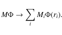
|
(24) |
Here, the matrix M projects a weighted combination of the
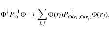
|
(25) |
and can be calculated from the primordial power spectrum
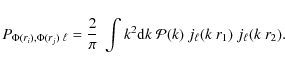
|
(26) |
To tighten the constraints on
The computational speed of a complete implementation is limited by
harmonic transforms that scale as
![]() .
.
8 Summary
In this paper, we developed two methods to infer the amplitude of the
non-Gaussianity parameter
![]() from a data set within a Bayesian approach. We
focused on the so called local type of non-Gaussianity and derived an expression
for the joint probability distribution of
from a data set within a Bayesian approach. We
focused on the so called local type of non-Gaussianity and derived an expression
for the joint probability distribution of
![]() and the primordial
curvature perturbations,
and the primordial
curvature perturbations, ![]() .
Despite the methods are of general
validity, we tailored our discussion to the case example of CMB data
analysis.
.
Despite the methods are of general
validity, we tailored our discussion to the case example of CMB data
analysis.
We developed an exact Markov Chain sampler that generates correlated samples from the joint density using the Hamiltonian Monte Carlo approach. We implemented the HMC sampler and applied it to a toy model consisting of simulated measurements of a 1D sky. These simulations demonstrate that the recovered posterior distribution is consistent with the level of simulated non-Gaussianity.
With two approximations that exploit the fact that the non-Gaussian
contribution to the signal is next order in perturbation theory, we
find a far more computationally efficient Monte Carlo sampling
algorithm that produces independent samples from the
![]() posterior. The regime of applicability for this approximation is for
data with high signal-to-noise and weak non-Gaussianity.
posterior. The regime of applicability for this approximation is for
data with high signal-to-noise and weak non-Gaussianity.
By comparison to the exact HMC sampler, we show that our approximate
algorithm reproduces the posterior location and shape in its regime of
applicability. If non-zero
![]() is not supported by the data the
method is biased towards Gaussianity. The approximate posterior more
strongly prefers zero
is not supported by the data the
method is biased towards Gaussianity. The approximate posterior more
strongly prefers zero
![]() compared to non-zero values than the exact
posterior, as expected given the nature of the approximations which
Gaussianize the prior. This method is therefore only applicable if the
data contains sufficient support for the presence of non-Gaussianity
essentially overruling the preference for Gaussianity in our
approximate prior.
compared to non-zero values than the exact
posterior, as expected given the nature of the approximations which
Gaussianize the prior. This method is therefore only applicable if the
data contains sufficient support for the presence of non-Gaussianity
essentially overruling the preference for Gaussianity in our
approximate prior.
Our efficient method enables us to perform a Monte Carlo study of the
behavior of the posterior density for our toy model data with high
signal-to-noise per pixel. We found that the width of the posterior
distribution does not change as a function of the level of non-Gaussianity in
the data, contrary to the frequentist estimator where there is an
additional,
![]() dependent, variance component
(Liguori et al. 2007; Creminelli et al. 2007). Our results suggest
that this may be an advantage of the Bayesian approach compared to the
frequentist approach, motivating further study of the application of
Bayesian statistics to the search for primordial local non-Gaussianity in
current and future CMB data.
dependent, variance component
(Liguori et al. 2007; Creminelli et al. 2007). Our results suggest
that this may be an advantage of the Bayesian approach compared to the
frequentist approach, motivating further study of the application of
Bayesian statistics to the search for primordial local non-Gaussianity in
current and future CMB data.
We close on a somewhat philosophical remark. Even though we chose a Gaussian prior approximation for expediency, it may actually be an accurate model of prior belief for many cosmologists since canonical theoretical models predict Gaussian perturbations. From that perspective our fast, approximate method may offer some (philosophically interesting) insight into the question ``what level of signal-to-noise in the data is required to convince someone of the presence of non-Gaussianity whose prior belief is that the primordial perturbations are Gaussian?''
AcknowledgementsWe thank the anonymous referee for the comments which helped to improve the presentation of our results. We are grateful to Rob Tandy for doing initial tests on detecting primordial non-Gaussianity in reconstructed sky maps. We thank Anthony J. Banday for useful conversations. B.D.W. is partially supported by NSF grants AST 0507676 and AST 07-08849. B.D.W. gratefully acknowledges the Alexander v. Humboldt Foundation's Friedrich Wilhelm Bessel Award which funded part of this work.
References
- Acquaviva, V., Bartolo, N., Matarrese, S., & Riotto, A. 2003, Nucl. Phys. B, 667, 119 [NASA ADS] [CrossRef] [Google Scholar]
- Alishahiha, M., Silverstein, E., & Tong, D. 2004, Phys. Rev. D, 70, 123505 [NASA ADS] [CrossRef] [Google Scholar]
- Babich, D. 2005, Phys. Rev. D, 72, 043003 [NASA ADS] [CrossRef] [Google Scholar]
- Babich, D., Creminelli, P., & Zaldarriaga, M. 2004, J. Cosmol. Astro-Part. Phys., 8, 9 [Google Scholar]
- Bartolo, N., Komatsu, E., Matarrese, S., & Riotto, A. 2004, Phys. Rep., 402, 103 [NASA ADS] [CrossRef] [Google Scholar]
- Bean, R., Dunkley, J., & Pierpaoli, E. 2006, Phys. Rev. D, 74, 063503 [NASA ADS] [CrossRef] [Google Scholar]
- Bond, J. R., Jaffe, A. H., & Knox, L. 1998, Phys. Rev. D, 57, 2117 [NASA ADS] [CrossRef] [Google Scholar]
- Carvalho, P., Rocha, G., & Hobson, M. P. 2009, MNRAS, 393, 681 [NASA ADS] [CrossRef] [Google Scholar]
- Creminelli, P., Nicolis, A., Senatore, L., Tegmark, M., & Zaldarriaga, M. 2006, J. Cosmol. Astro-Part. Phys., 5, 4 [Google Scholar]
- Creminelli, P., Senatore, L., & Zaldarriaga, M. 2007, J. Cosmol. Astro-Part. Phys., 3, 19 [NASA ADS] [CrossRef] [Google Scholar]
- Duane, S., Kennedy, A. D., Pendleton, B. J., & Roweth, D. 1987, Phys. Lett. B, 195, 216 [NASA ADS] [CrossRef] [Google Scholar]
- Elsner, F., & Wandelt, B. D. 2009, ApJS, 184, 264 [NASA ADS] [CrossRef] [Google Scholar]
- Enqvist, K., & Sloth, M. S. 2002, Nucl. Phys., B626, 395 [Google Scholar]
- Eriksen, H. K., Dickinson, C., Lawrence, C. R., et al. 2006, ApJ, 641, 665 [NASA ADS] [CrossRef] [Google Scholar]
- Eriksen, H. K., Dickinson, C., Jewell, J. B., Banday, A. J., Górski, K. M., & Lawrence, C. R. 2008, ApJ, 672, L87 [NASA ADS] [CrossRef] [Google Scholar]
- Gelman, A., & Rubin, D. B. 1992, Stat. Sci., 7, 457 [Google Scholar]
- Guth, A. H. 1981, Phys. Rev. D, 23, 347 [NASA ADS] [CrossRef] [MathSciNet] [Google Scholar]
- Hajian, A. 2007, Phys. Rev. D, 75, 083525 [NASA ADS] [CrossRef] [Google Scholar]
- Hinshaw, G., Weiland, J. L., Hill, R. S., et al. 2009, ApJS, 180, 225 [NASA ADS] [CrossRef] [Google Scholar]
- Hobson, M. P., & McLachlan, C. 2003, MNRAS, 338, 765 [NASA ADS] [CrossRef] [Google Scholar]
- Jewell, J., Levin, S., & Anderson, C. H. 2004, ApJ, 609, 1 [NASA ADS] [CrossRef] [Google Scholar]
- Khoury, J., Ovrut, B. A., Steinhardt, P. J., & Turok, N. 2001, Phys. Rev. D, 64, 123522 [NASA ADS] [CrossRef] [MathSciNet] [Google Scholar]
- Komatsu, E., & Spergel, D. N. 2001, Phys. Rev. D, 63, 063002 [NASA ADS] [CrossRef] [Google Scholar]
- Komatsu, E., Spergel, D. N., & Wandelt, B. D. 2005, ApJ, 634, 14 [NASA ADS] [CrossRef] [Google Scholar]
- Lewis, A., & Bridle, S. 2002, Phys. Rev. D, 66, 103511 [NASA ADS] [CrossRef] [Google Scholar]
- Liguori, M., Yadav, A., Hansen, F. K., et al. 2007, Phys. Rev. D, 76, 105016 [NASA ADS] [CrossRef] [Google Scholar]
- Linde, A. D. 1982, Phys. Lett. B, 108, 389 [Google Scholar]
- Lyth, D. H., Ungarelli, C., & Wands, D. 2003, Phys. Rev. D, 67, 023503 [NASA ADS] [CrossRef] [Google Scholar]
- Maldacena, J. M. 2003, JHEP, 05, 013 [NASA ADS] [CrossRef] [Google Scholar]
- Moroi, T., & Takahashi, T. 2001, Phys. Lett. B, 522, 215 [NASA ADS] [CrossRef] [Google Scholar]
- Senatore, L. 2005, Phys. Rev. D, 71, 043512 [NASA ADS] [CrossRef] [Google Scholar]
- Smith, K. M., Senatore, L., & Zaldarriaga, M. 2009, J. Cosmol. Astro-Part. Phys., 9, 6 [Google Scholar]
- Spergel, D. N., Bean, R., Doré, O., et al. 2007, ApJS, 170, 377 [NASA ADS] [CrossRef] [Google Scholar]
- Steinhardt, P. J., & Turok, N. 2002, Phys. Rev. D, 65, 126003 [NASA ADS] [CrossRef] [Google Scholar]
- Taylor, J. F., Ashdown, M. A. J., & Hobson, M. P. 2008, MNRAS, 389, 1284 [NASA ADS] [CrossRef] [Google Scholar]
- Tegmark, M. 1997, Phys. Rev. D, 55, 5895 [Google Scholar]
- Trotta, R. 2007, MNRAS, 375, L26 [NASA ADS] [Google Scholar]
- Verde, L., Wang, L., Heavens, A. F., & Kamionkowski, M. 2000, MNRAS, 313, 141 [NASA ADS] [CrossRef] [Google Scholar]
- Wandelt, B. D., Larson, D. L., & Lakshminarayanan, A. 2004, Phys. Rev. D, 70, 083511 [NASA ADS] [CrossRef] [Google Scholar]
- Yadav, A. P., & Wandelt, B. D. 2005, Phys. Rev. D, 71, 123004 [NASA ADS] [CrossRef] [Google Scholar]
- Yadav, A. P. S., Komatsu, E., & Wandelt, B. D. 2007, ApJ, 664, 680 [NASA ADS] [CrossRef] [Google Scholar]
Footnotes
- ...
tools
![[*]](/icons/foot_motif.png)
- E.g. as described in Lewis & Bridle (2002).
All Figures
|
|
Figure 1:
Examples of reconstructed potentials
|
| Open with DEXTER | |
| In the text | |
|
|
Figure 2:
Examples of a constructed posterior distribution for
|
| Open with DEXTER | |
| In the text | |
|
|
Figure 3:
Build-up of the posterior distribution of
|
| Open with DEXTER | |
| In the text | |
|
|
Figure 4:
Properties of the sampler. Left panel: shown is the
distribution of the derived mean values of
|
| Open with DEXTER | |
| In the text | |
| |
Figure 5:
Impact of the signal-to-noise ratio on the approximate sampling
scheme. Left panel: example of a constructed posterior
distribution for S/N = 10. Middle panel: analysis of the
same data set, but for S/N = 0.5. At high noise level, the
distribution becomes too narrow and systematically shifted towards
|
| Open with DEXTER | |
| In the text | |
|
|
Figure 6:
Example
|
| Open with DEXTER | |
| In the text | |
|
|
Figure 7:
Performance of the Hamilton Monte Carlo sampler. Left panel:
analysis of the data set of Fig. 3 using the HMC
sampler. Here, 15 000 samples were draw. Right panel: the
autocorrelation function of
|
| Open with DEXTER | |
| In the text | |
Copyright ESO 2010
Current usage metrics show cumulative count of Article Views (full-text article views including HTML views, PDF and ePub downloads, according to the available data) and Abstracts Views on Vision4Press platform.
Data correspond to usage on the plateform after 2015. The current usage metrics is available 48-96 hours after online publication and is updated daily on week days.
Initial download of the metrics may take a while.