| Issue |
A&A
Volume 512, March-April 2010
|
|
|---|---|---|
| Article Number | A39 | |
| Number of page(s) | 13 | |
| Section | Planets and planetary systems | |
| DOI | https://doi.org/10.1051/0004-6361/200913551 | |
| Published online | 25 March 2010 | |
Using the Sun to estimate Earth-like planets detection capabilities
II. Impact of plages
N. Meunier - M. Desort - A.-M. Lagrange
Laboratoire d'Astrophysique de Grenoble, Observatoire de Grenoble, Université Joseph Fourier, CNRS, UMR 5571, 38041 Grenoble Cedex 09, France
Received 26 October 2009 / Accepted 10 December 2009
Abstract
Aims. Stellar activity produced by spots and plages affects
the radial velocity (RV) signatures. Because even low activity stars
would produce such a signal, it is crucial to determine how it
influences our ability to detect small planetary signals such as those
produced by Earth-mass planets in the habitable zone (HZ). In a recent
paper, we investigated the impact of sunlike spots. We aim here to
investigate the additional impact of plages.
Methods. We used the spot and plage properties over a solar
cycle to derive the RV that would be observed if the Sun was seen
edge-on. The RV signal comes from the photometric contribution of spots
and plages and from the attenuation of the convective blueshift in
plages. We analyzed the properties of the RV signal at different
activity levels and compared it with commonly used activity indicators
such as photometry and the Ca index. We also compared it with the
signal that would be produced by an Earth-mass planet in the HZ.
Results. We find that the photometric contributions of spots and
plages to the RV signal partially balance each other out, so that the
residual signal is comparable to the spot signal. However, the plage
contribution due to the convective blueshift attenuation dominates the
total signal, with an amplitude over the solar cycle of about
8-10 m/s. Short-term variations are also significantly greater
than the spot and plage photometric contribution. This contribution is
very strongly correlated with the Ca index on the long term, which may
be a way to distinguish between stellar activity and a planet.
Conclusions. Providing a very good temporal sampling and
signal-to-noise ratio, the photometric contribution of plages and spots
should not prevent detection of Earth-mass planets in the HZ.
However, the convection contribution makes such a direct detection
impossible, unless its effect can be corrected for by methods that
still need to be found. We show that it is possible to identify the
convection contribution if the sensitivity is good enough, for example,
by using activity indicators.
Key words: techniques: radial velocities - starspots - planetary systems - stars: activity
1 Introduction
Among other techniques, the radial velocity (hereafter RV) technique has been very successful in detecting exoplanets. The increasing sensitivity of new instruments (for example, Espresso on the VLT or Codex on the E-ELT) is expected to give access to increasingly lower planet masses (down to Earth-like masses); however, it also makes the observed RV signal sensitive to other sources than planets, such as stellar activity and pulsations.
The influence of spots on the RV and bisector were first studied by Saar & Donahue (1997) and Hatzes (2002). This was followed by the precise study of the influence of a single spot on the signal (Desort et al. 2007) in various stellar conditions such as inclinations or angular rotation rates. In Lagrange et al. (2010),
hereafter Paper I, we simulated the RV signal due to spots that
would be detected if the Sun was observed edge-on over a long period
(typically one solar cycle) with different temporal samplings (between
one day and 20 days) with only a few gaps. The advantage of such
an approach compared to the previous ones is that we could take the
full complexity of the activity pattern into account (structures,
spatial distribution, temporal variations), because the signal from
spots on various positions on the disk can partially balance each other
out. Our approach also allows us to study the temporal behavior of the
signal (such as with periodograms, which are also very useful tools to
detect planets in the RV signal). We derived a typical RV signal of
0.45 m/s (rms), with maximum peaks at ![]() 2 m/s, especially during the solar maximum (
2 m/s, especially during the solar maximum (
![]() ). During the solar minimum (
). During the solar minimum (
![]() ), the rms falls to 0.16 m/s with maximum peaks at
), the rms falls to 0.16 m/s with maximum peaks at ![]() 0.6 m/s.
Then we estimated the impact of these spots on the detection of
Earth-like planets and showed that a very good temporal sampling over a
long period was mandatory for detecting Earth-mass planets in the
habitable zone, depending on the cycle phase.
0.6 m/s.
Then we estimated the impact of these spots on the detection of
Earth-like planets and showed that a very good temporal sampling over a
long period was mandatory for detecting Earth-mass planets in the
habitable zone, depending on the cycle phase.
However, spots are not the only source of RV variations. The presence of bright plages also induces a variable signal in RV, as for spots. They are well-known on the Sun, but there are indirect indications that they are also present on other stars, as they sometimes dominate the photometry (e.g. Lockwood et al. 2007). Their contrast in temperature is less than for spots, but their area is much larger. Their contribution is therefore expected to be significant. Such a contribution to the RV has never been studied in precise detail. Because they are bright, we expect plages located at the same position as spots to produce an RV signal anti-correlated with the one from the spot (see Paper I). However, because they are not localized exactly at the same position (in addition to their different spatial extension) and have a position-dependent contrast, and because in practice there is no one-to-one correspondence between the two types of structures (the plage to spot area ratio presents a very large dispersion, Chapman et al. 2001), the residual signal will be significant. In addition, there are many small plage-like structures outside active regions, called the network, contributing significantly to the photometric variations of the Sun. It is crucial to study the two contributions (spots and plages) separately and in detail because the respective contributions of plages and spots may be different on other stars (Lockwood et al. 2007).
Another contribution of plages comes from the attenuation of the convective blueshift (due to the presence of granulation, e.g. Gray 2009) when magnetic field is present. Rough estimates have been made on individual lines (Kürster et al. 2003; Saar 2003; Saar & Donahue 1997) but the impact on the RV variations derived from the cross-correlation function (CCF) has not been studied yet.
The objective of this paper is therefore to estimate the contribution of plages to the RV signal (either from the photometry or the convection), to compare it to the signal produced by spots at the same time, and to study the resulting signal. As in Paper I, we consider a Sun seen edge-on over a solar cycle. In Sect. 2, we describe in detail the data set (spots and plages), the data processing, and the observables we obtain. Special care is given to the comparison with the observed photometry (total solar irradiance) in order to validate the parameters used to make the simulation. The resulting RV are analyzed in Sect. 3 and compared with other observables (photometry, Ca index) in Sect. 4. In Sect. 5, we study the influence of this signal on Earth-like planet detection, and conclude in Sect. 6.
2 Description of the simulations
In this section we first describe the input data: the list of sunspots and plages that is used as input to our simulation tool; the way we derive the temperature contrasts for these structures; the influence of convective inhomogeneities. Then we briefly describe our simulation and the produced observables, which are similar to what was done in Paper I.
2.1 Input data
To get a good temporal sampling of plages, we used MDI/SOHO magnetograms (Scherrer et al. 1995) between May 5, 1996 (julian day 2450209) and October 7, 2007 (julian day 2454380). This covers a solar cycle with a temporal sampling of about 1 day. We therefore used a different sunspot data set from Paper I to cover the full plage data set, although there is a significant overlap between julian days 2450209 and 2453004. We chose the sunspot group data provided by USAF/NOAA over the same period (http://www.ngdc.noaa.gov/stp/SOLAR/).
This sunspot data set has a few gaps. Some of them correspond to days without any spot while others are true gaps in the data. We removed the latter from the MDI data set by checking the Wolf number. In the following, there are therefore plage structures every day, but in some cases there may be no spot on the Sun surface. This leads to 3586 days, for a total duration of 4171 days (i.e. a 86% coverage, which is similar to what we had for spots in Paper I).
![\begin{figure}
\par\includegraphics[width=12cm,clip]{13551fig1.ps}
\end{figure}](/articles/aa/full_html/2010/04/aa13551-09/img6.png)
|
Figure 1: Upper panel: MDI magnetogram for September 14, 2002 at 4:48 UT (left) and Meudon photospheric spectroheliogram at 6:41 UT (right). Lower panel: simulated map showing the plages derived from the magnetogram with a contrast increased by a factor 10 for clarity ( left) and the spots from the USAF/NOAA data set at 12:40 UT (right). |
| Open with DEXTER | |
The spot data are used without any further processing and provide 35207 sunspot groups, with the smallest size 10 ppm (of the solar hemisphere). This size corresponds to a radius of 3.1 Mm, assuming a circular shape. We note that the surface coverage of the Debrecen data used in Paper I is larger by a factor of about 1.57 when comparing the same days. The impact of this difference is investigated in the next section.
Plages (in active regions) and network structures (bright magnetic
structures outside active regions) are extracted from MDI magnetograms
by applying a threshold of 100 G for ![]() up to 72
up to 72![]() (with
(with ![]() the angle between the line-of-sight and the normal to the solar
surface) in order to avoid the noise close to the limb. This threshold
is quite conservative for limiting the influence of the noise (about
20 G), and is slightly larger than the one used by Fligge et al. (2000)
on the same data. For the same purpose, the smallest structures are
eliminated. The smallest size is then 3 ppm (of the solar
hemisphere), which corresponds to a radius of 1.7 Mm assuming a
circular shape. This is smaller than the smallest spots we consider
because we also include network structures and not only plages from
active regions. This leads to 1803344 structures, from the quiet
network to large plages in active regions. The relative contribution of
plages and network structures is discussed in Sect. 2.3.2.
the angle between the line-of-sight and the normal to the solar
surface) in order to avoid the noise close to the limb. This threshold
is quite conservative for limiting the influence of the noise (about
20 G), and is slightly larger than the one used by Fligge et al. (2000)
on the same data. For the same purpose, the smallest structures are
eliminated. The smallest size is then 3 ppm (of the solar
hemisphere), which corresponds to a radius of 1.7 Mm assuming a
circular shape. This is smaller than the smallest spots we consider
because we also include network structures and not only plages from
active regions. This leads to 1803344 structures, from the quiet
network to large plages in active regions. The relative contribution of
plages and network structures is discussed in Sect. 2.3.2.
The structures extracted from the magnetograms using this simple segmentation also include spots of course. With the present context, this is not critical, however, since the surface coverage of spots is much smaller. Typically, the filling factor of spots (determined from the USAF data above) represents about 6% of the filling factor of structures determined from the magnetograms. Furthermore, modifications of the threshold used to identify plages lead to modification of that filling factor by about 10% in the case of large structures and up to 20% for small network features, without changing their visual identification significantly. This gives an idea of the uncertainty on the filling factor. The influence of this variation is also investigated in the next section.
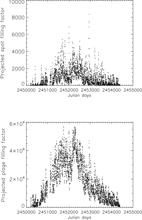
The first input to our simulation tool (for both spots and plages) then consists in the list of structures: size in ppm of the solar hemisphere (before correction for projection effects), latitude, and longitude. The projected filling factors are shown in Fig. 2. The correlation between the spot and plage filling factors is 0.77. This reflects the correlation between the two, both on long (cycle) and short time scales (rotation), as active regions usually include spots, but also the large dispersion of the plage-to-spot size ratio and the inclusion of the network structures (not spatially correlated with spots as they are located outside active regions). The plage filling factor is about one order of magnitude more than the spot filling factor.
2.2 Contrast choices
2.2.1 Spot and plage observed contrasts
There is a large dispersion in the literature concerning the spot and plage contrasts. There is also a large temperature difference from one structure to the next. It is therefore difficult to directly use the published contrasts found in the literature (for example Frazier 1971; Lawrence 1988; Ermolli et al. 2007), because they are very sensitive to the way plages are defined. The large dispersion between individual plages, as well as the differences between plages and network structures (Ortiz et al. 2006; Worden et al. 1998; Foukal et al. 1991; Ortiz et al. 2002) also adds to the uncertainty of these measurements. To realize a consistent simulation, we computed the photometric contribution of each kind of structure (spots, plages, network) and compared it with the observed total solar irradiance (hereafter TSI). In the following we use the TSI compiled by Claus Fröhlich and Judith Lean (http://www.ngdc.noaa.gov/stp/SOLAR/) for the 1996-2003 period and described in Fröhlich & Lean (1998). This comparison is therefore made over 2263 points.
In Paper I, we used a spot temperature deficit of 550 K, as
this lies well within the range of observations and simulations (e.g. Krivova et al. 2003; Chapman et al. 1994; Fligge et al. 2000). The situation is more complex for plages. We can either use a shape such as the one used by Lanza et al. (2004,2007) and in Paper I, i.e. a temperature excess as a function of 1-![]() (where
(where
![]() ). We can also use a slightly more complex function such as in Unruh et al. (1999) and used by Fligge et al. (1998,2000)
to reconstruct the solar irradiance, to account for the difference from
zero contrast at disk center. In the following, we use a second-degre
polynomial starting with a shape similar to the one modeled by Unruh et al. (1999), as it gives a slightly better
). We can also use a slightly more complex function such as in Unruh et al. (1999) and used by Fligge et al. (1998,2000)
to reconstruct the solar irradiance, to account for the difference from
zero contrast at disk center. In the following, we use a second-degre
polynomial starting with a shape similar to the one modeled by Unruh et al. (1999), as it gives a slightly better ![]() when comparing the simulated irradiance to the observed one (see next section).
when comparing the simulated irradiance to the observed one (see next section).
2.2.2 Determination of the spot and plage contrast
|
Figure 2: Upper panel: projected spot filling factor versus time, in ppm of the solar disk. Lower panel: same for plages. |
| Open with DEXTER | |

|
Figure 3:
Upper panel: plage temperature excess versus |
| Open with DEXTER | |
We used the following procedure to determine the spot and plage contrasts.
We first consider a spot temperature deficit![]()
![]() K and a plage contrast
K and a plage contrast![]()
![]() -0.563
-0.563 ![]() +0.270
+0.270 ![]() K, which corresponds to the contrast provided by Unruh et al. (1999)
for wavelengths in the range 470-550 nm. We then computed a
contrast at 600 nm assuming a Planck law, which leads to estimate
the contribution of spots and plages to the TSI. We chose
600 nm for reference because that is where the contrast is close
to the average contrast over 350-1000 nm, representative of the
bolometric value (Gondoin 2008), hence the TSI.
K, which corresponds to the contrast provided by Unruh et al. (1999)
for wavelengths in the range 470-550 nm. We then computed a
contrast at 600 nm assuming a Planck law, which leads to estimate
the contribution of spots and plages to the TSI. We chose
600 nm for reference because that is where the contrast is close
to the average contrast over 350-1000 nm, representative of the
bolometric value (Gondoin 2008), hence the TSI.
This leads to two series,
![]() and
and
![]() ,
respectively representing the contribution of dark and bright features
to the solar irradiance, in fractions of the TSI of the quiet Sun (i.e.
contrasts). When multiplied by the quiet Sun irradiance
,
respectively representing the contribution of dark and bright features
to the solar irradiance, in fractions of the TSI of the quiet Sun (i.e.
contrasts). When multiplied by the quiet Sun irradiance
![]() they allow a direct comparison with the observed TSI
they allow a direct comparison with the observed TSI
![]() (in W/m2) by computing
(in W/m2) by computing

which sums the contributions of spots, plages (including the network), and quiet Sun respectively. We can adjust

and N the number of points,
The final reconstructed irradiance versus the observed TSI will be
shown in Sect. 2.5, as here we have made a simplified computation
to correct for projection effects, we attribute to each structure the
value of ![]() corresponding to the center of the structure, while in the following we
build maps of the solar surface. We also neglect the center-to-limb
darkening (which will be taken considered in Sect. 2.5 where we
make a more precise computation of
corresponding to the center of the structure, while in the following we
build maps of the solar surface. We also neglect the center-to-limb
darkening (which will be taken considered in Sect. 2.5 where we
make a more precise computation of
![]() ). Figure 5
shows the contribution of spots and plages to the irradiance, as well
as the simulated irradiance used here to derive the set of parameters.
Our results are quite similar to those of Fröhlich & Lean (1998), and we reproduce the observed irradiance.
). Figure 5
shows the contribution of spots and plages to the irradiance, as well
as the simulated irradiance used here to derive the set of parameters.
Our results are quite similar to those of Fröhlich & Lean (1998), and we reproduce the observed irradiance.
2.2.3 Uncertainties
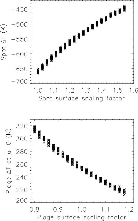
To study the influence of our input data set (USAF sunspot group and plage extraction from MDI magnetograms), we explored the parameter space related to the structure sizes by applying a certain scaling factor to them, which should represent the uncertainty we have on the structure sizes. For spots, we applied scaling factors between 1 (original USAF values) and 1.57 (corresponding the Debrecen filling factor), i.e. we allow the spot size to vary by about 50%. The smaller filling factor in the USAF catalog may stem from missing very small spots (Balmaceda et al. 2009), at least partially. The correction also included a small dependence on the size, as we have been able to compare specific regions, which shows that, as expected, the correction is relatively large for small structures. For plages, we applied scaling factors between 0.8 and 1.2, which takes the assumption concerning the inclusion of spots into account, as well as a margin for the choice of the threshold. We therefore allowed the plage and network sizes to vary byFor each new series of spot and plage sizes, we searched for the contrasts that provide the best fit to the observed TSI, following the method described in Sect. 2.2.2. Indeed, at first order, if one slightly overestimates the plage areas, for example, it can be compensated for a larger temperature excess. This is true for the reconstitution of the solar irradiance and also for RV computations as it also is a photometric effect. The quiet-Sun solar irradiance is fixed to our best value above, as it is very robust.
The results are as follows. The corresponding
![]() ranges between -670 K (for a spot scaling factor of 1) and
-450 K (for a spot scaling factor of 1.57), with a strong
correlation as expected (see Fig. 4). At
ranges between -670 K (for a spot scaling factor of 1) and
-450 K (for a spot scaling factor of 1.57), with a strong
correlation as expected (see Fig. 4). At ![]() ,
,
![]() varies between
varies between ![]() 315 K (for a plage scaling factor of 0.8) and
315 K (for a plage scaling factor of 0.8) and ![]() 215 K (for a plage scaling factor of 1.2), and between
215 K (for a plage scaling factor of 1.2), and between ![]() 43 K and
43 K and ![]() 29 K at
29 K at ![]() ,
here again with a strong anticorrelation because the areas and
temperature excess compensate for each other. This anticorrelation is
shown in Fig. 4 for
,
here again with a strong anticorrelation because the areas and
temperature excess compensate for each other. This anticorrelation is
shown in Fig. 4 for ![]() .
Figure 3 also shows the plage-temperature excess (and contrast at 600 nm) versus
.
Figure 3 also shows the plage-temperature excess (and contrast at 600 nm) versus ![]() for the whole domain.
Over the whole domain, the
for the whole domain.
Over the whole domain, the ![]() remains very low. It does not show any systematic effect when changing the plage surface. The
remains very low. It does not show any systematic effect when changing the plage surface. The ![]() is, however, smaller for the spot scaling factor of 1 compared
to 1.57. It is also very close to the minimum as a test of a few
values below 1 for the spot scaling factor shows that the
is, however, smaller for the spot scaling factor of 1 compared
to 1.57. It is also very close to the minimum as a test of a few
values below 1 for the spot scaling factor shows that the ![]() then increases again.
then increases again.
Finally, we note that in Paper I we used the Debrecen data set, which corresponds to the spot-surface scaling factor of ![]() 1.6 in Fig. 4.
We used a spot temperature deficit of -550 K, which lies in the
middle of our range, instead of -450 K. We therefore expect our
spot RV signal to be weaker by about 20% than that of
Paper I, in which the spot temperature deficit could not be
validated precisely using the observed irradiance because plage were
not taken into account.
1.6 in Fig. 4.
We used a spot temperature deficit of -550 K, which lies in the
middle of our range, instead of -450 K. We therefore expect our
spot RV signal to be weaker by about 20% than that of
Paper I, in which the spot temperature deficit could not be
validated precisely using the observed irradiance because plage were
not taken into account.
We are therefore confident that our choice of temperature contrasts will provide the correct amplitude of the RV signal, as we are including two crucial ingredients in our simulation: a correct amplitude due to a good combination between area and contrast, as checked by the comparison with the observed irradiance, and a realistic temporal evolution of structures thanks to the temporal sampling and coverage.
|
Figure 4:
Upper panel: spot temperature deficit versus the spot-surface
scaling factor for the explored range of scaling factors (see text for
details). For a given spot-surface scaling factor, the various points
correspond to different plage-surface scaling factors. Bottom panel: same for plages at |
| Open with DEXTER | |
|
Figure 5: First panel: reconstructed spot contribution to irradiance. Second panel: reconstructed plage contribution to irradiance. Third panel: total reconstructed irradiance. Fourth panel: observed irradiance. |
| Open with DEXTER | |
2.3 Convective inhomogeneities
2.3.1 Estimation of convective shifts
In addition to the photometric effect described above, another effect can lead to RV and bisector variations. The presence of convection in the photosphere produces a blueshift of spectral lines, as well as a distortion of these lines (e.g. Livingston et al. 1999; Dravins 1999; Dravins et al. 1981; Dravins 1982). This comes from the correlation between velocities and brightnesses in granules. Granules are convective cells at the 1 Mm scale, in which upward motions associated to bright area occupy a larger surface than downward motion area (dark lanes), leading to blueshifts and to line distortion. However, where magnetic field is present, it is well known that convection is affected, and is greatly reduced (e.g. Hanslmeier et al. 1991; Schmidt et al. 1988; Title et al. 1987). This strongly impacts the lines by locally modifying their shape and producing a redshift that compensates for the convective blueshift (Hanslmeier et al. 1994; Guenther & Mattig 1991; Cavallini et al. 1985; Brandt & Solanki 1990; Hanslmeier & Mattig 1990; Immerschitt & Schroeter 1989). This influence of the magnetic field on the lines has also been modelled by Marquez et al. (1996); therefore, we do expect this blueshift to be modified by the presence of plages (as well as spots, but their contribution is small as they represent a much smaller surface and are darker).
In the following, we estimate the amplitude of the convective blueshift
in the quiet Sun. The convective blueshift largely depends on the line
depth, and a large dispersion is present in the literature as most
studies focus on a small number of lines. We have used the detailed
results of Gray (2009)
for the Sun and derived a blueshift as a function of the line depths
using a linear function. Then, on the solar spectrum obtained by
Delbouille, Neven, and Roland (retrieved from the BASS2000 data base),
we have identified the lines in our spectral range of interest,
retrieved their position and depth, then simulated a spectrum in which
each line has the same depth but is shifted by a different amount
according to its depth and following Gray (2009).
We used a linear relation between the line depth and the blueshift,
which is extrapolated to lines outside the range of depth considered by
Gray (2009). Finally, we computed the shift that
would result from a cross-correlation applied on such a spectrum. We
therefore consider the distribution of line depths in the spectrum and
that cross-correlation functions (used later to derive the RV) are
more sensitive to deep lines than weak lines. This produces a
convective blueshift corresponding to the integrated light of about
200 m/s that is representative of the whole spectrum. The local
(vertical) convective blueshift is therefore 285 m/s (the
corresponding factor being the result of projection effects combined to
the center-to-limb darkening). It is similar to the value used by Kürster et al. (2003) derived from Dravins (1999), but higher than the value considered by Saar (2003), about 90 m/s for the ![]() we consider.
we consider.
Gray (2009) studied the blueshift only for a quiet Sun (or star). On the other hand, Brandt & Solanki (1990)
studied the line shape and shifts for different magnetic filling
factors (including the quiet Sun), by observing at different positions
in a plage. They find a blueshift in plages which is 1/3 of the
value in the quiet Sun. We therefore use in the following an
attenuation of the convective blueshift of 2/3 of our values, i.e.
190 m/s. The results of Cavallini et al. (1985) are also compatible with this result. We expect the attenuation to be around zero in spot umbra (Martinez Pillet et al. 1997; Solanki 1986),
but the contribution of the umbra is very small. Given that the spread
in convective blueshift associated to plages in the literature, about
50 m/s, we consider that, in the presence of plages and network
(see next section), the convective blueshift is attenuated down to
190 m/s, with an uncertainty of ![]() 50 m/s.
We neglect in this work the contribution of the Evershed effect (mostly
associated to spot penumbra) and supergranulation, because we expect
them to only increase slightly the jitter on scales from days to weeks.
50 m/s.
We neglect in this work the contribution of the Evershed effect (mostly
associated to spot penumbra) and supergranulation, because we expect
them to only increase slightly the jitter on scales from days to weeks.
2.3.2 Notes on the convective shifts
All solar observations of the line distortions and shifts due to magnetic fields have focused on plages. Our data set includes a significant contribution from the network. We also know that some abnormal granulation is associated to it, for example, to network bright points (e.g. Muller et al. 1989). More recently, Morinaga et al. (2008) have shown the suppression of convection around small magnetic concentrations; however, there is no specific study of the lineshift associated to the network that we are aware of. In the following, we consider the RV signal associated to all structures, but will also estimate it for regions of a signifiant size only in order to test the possible range of variation. There is of course a continuum in size from the largest active regions to the small network structures (Meunier 2003), but only considering sizes above 100 ppm (corresponding to a radius of 10 Mm) would probably give a good estimation of a lower limit for the convection contribution to the RV. This is discussed in Sect. 3.3.2.
Finally, it should be noted that the final RV signal due to convective
inhomogeneities is sensitive to the actual areas of structures and to
the ![]() we consider. As before, for area and temperatures, there is a trade-off
between the two. However, unlike the temperature, we do not have the
possibility of testing it independently.
we consider. As before, for area and temperatures, there is a trade-off
between the two. However, unlike the temperature, we do not have the
possibility of testing it independently.
2.4 Simulated spectra
Simulated spectra are computed as described in Paper I. A rigid rotation of 1.9 km s-1 at the equator is assumed. For each type of structure (spots and plages), we build a 3D hemisphere map of the visible Sun seen edge-on. We assumed circular shapes in both cases, mostly for simplicity as we do not expect the shape to significantly impact on our result, and more importantly to be able to extrapolate easily to other stellar cases in future works. For the photometric contribution of magnetic structures, the resulting spectrum is then computed assuming that spots (respectively plages) emit a solar-like spectrum following a black body law with a temperature as described in the previous section. To take the convection into account, we consider a solar-like spectrum (black body with the photospheric temperature) shifted by a velocity perpendicular to the solar surface (which produces a redshift) of 190 m/s.
2.5 Computation of the observables
|
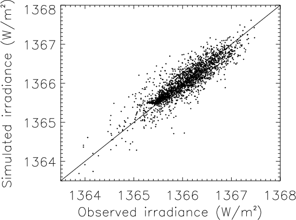
Figure 6: Total reconstructed irradiance versus the observed irradiance (W/m2). |
| Open with DEXTER | |
The observables are then computed using the SAFIR software (Galland et al. 2005) as on actual stellar spectra. In this paper we focus on the analysis of the RV. As in Paper I, computations were made only on one spectral order (order #31) as the whole process is very time consuming. We therefore obtained three series of RV, due to spots, to plages (and network) through their photometric contribution (hereafter the plage signal), and to the influence of plages on convection (hereafter the convection signal). The bisector velocity span (hereafter BVS) due to convective inhomogeneities has a very complex influence on the final line shape, and is not characterized with sufficient precision in the literature. We therefore only analyze the RV in this paper.
We also computed the photometry at 600 nm to check that we obtain the expected agreement. Figure 6 shows the good correlation (0.89) between the final simulated photometry and the observed TSI. The residual difference between the model and the simulation largely comes from the strong temperature variation from one structure to the next. However, we capture the essential variability of the photometry.
2.6 Simulation of an active star with a planet
To test the planet detectability providing the activity we model, we added the signal of a
1
![]() planet located at 1.2 AU (see Paper I) to the activity
signal, as well as some random noise at various level. This is analyzed
in Sect. 5.
planet located at 1.2 AU (see Paper I) to the activity
signal, as well as some random noise at various level. This is analyzed
in Sect. 5.
3 Results
In this section we present the different contributions to the RV signals over the whole period. In addition, in order to have a better idea of the dependence on the activity level, we also show the results for two 9-month periods as in Paper I: a period of low activity from July 1, 1996 (JD 2 450 266) to April 1, 1997 (JD 2 450 540), leading to 213 data points over 274 days, and a period of high activity from February 1, 2000 (JD 2 451 576) to November 1, 2000 (JD 2 451 850), leading to 274 data points, also over 274 days. They will be denoted as ``Low'' and ``High'', respectively, in the next figures and tables.
In addition to the total RV and the 3 individual components, we also discuss the contributions due to spots and plages separately (the total being denominated as the spot+plage signal) and compare them with the convection signal. This is important as they have a different origin (even if the convection signal relates to plages): on a star with similar plages but much weaker convection, the plage signal would remain the same but the convection signal would become very small.
3.1 RV variations
|
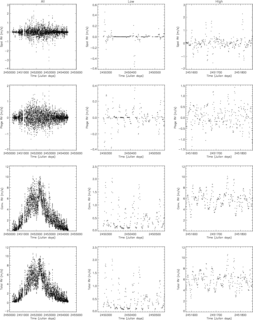
Figure 7: Left column: RV (m/s) for spot signal, plage signal, convection signal, and total ( From top to bottom), for the whole data set. Middle column: same for the low activity period. Right column: same for the high activity period. |
| Open with DEXTER | |
3.1.1 The spot and plage induced RV variations
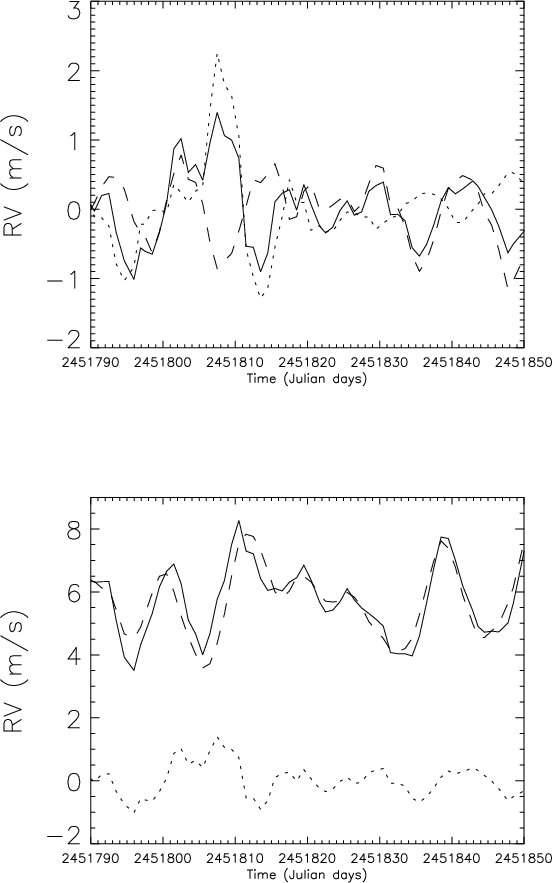
We first consider the individual time series of RV due to the photometric contributions of spots and plages. They are shown in Fig. 7. The amplitude of the spot signal is similar to what we found in Paper I (slightly smaller as expected), with maximum RV up to a few m/s during high activity periods. The RV is lower than 0.6 m/s during the minimum. The plage signal is, as expected, also higher during the high activity period (up to 1.6 m/s), i.e. about a factor two below the spot signal. The plage signal during the low activity period reaches 0.4 m/s, slightly below that of spots. It should be noted, however, that during that period the spot signal may be zero for an extended period of time, while the plage signal is always different from zero. Figure 8 (upper panel) shows the different contributions in more detail over a short period (60 days). As expected, the spot signal is partially compensated for that of plages (it was already true in the very simple computation made in Paper I), but not entirely. This can be explained as most active regions contain spots (leading to a compensation) but the area ratio between spots and plages varies (e.g. Chapman et al. 2001) and there are plages with no spot. Over the whole data set, the correlation between the spot and plage RV is indeed -0.47.
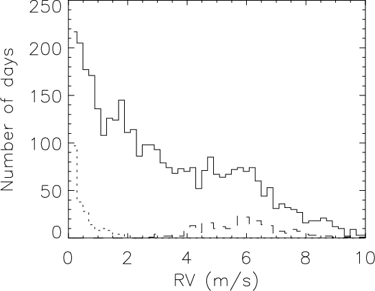
Figure 9 shows the distributions of RV for the spot and plage signals. The distributions are not Gaussian, as they show extended tails, and, in the case of spots, a sharp peak at zero RV (related to the significant number of days with no spot). The shape of the distribution is related to the shape of the solar cycle, i.e. to the variation in the activity level over time. A similar size distribution of structures with a constant activity level gives a Gaussian distribution. A sinusoidal shape for the solar cycle, for example, only leads to a small departure from the Gaussian shape while the proper shape gives a distribution similar to what is shown in Fig. 9. The rms RV for the whole period and the two periods corresponding to low and high activity are summarized in Table 1. The sum of the spot and plage RV is indicated as ``sp+pl''. It confirms that at all time spots and plages provide similar rms, but as they partially compensate for each other, the resulting rms is in fact similar to that of the individual components.
Figure 10 shows the
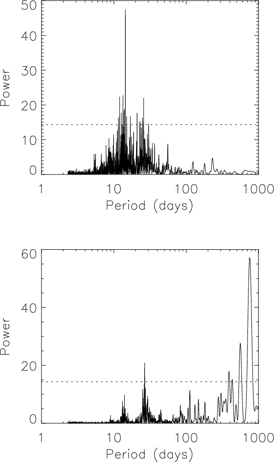
periodogram for the RV signal over the whole period for the spot+plage
signal. The peaks corresponding to half the rotation period are
strongly emphasized compared to the peaks at the rotation period. It
may stem from the presence of active longitudes separated by 180![]() as discussed in Paper I.
as discussed in Paper I.
3.1.2 The convection-induced RV variations
The convection signal is much stronger than the spot and plage ones as shown in Figs. 7 and 8. It is also fundamentally different, as it is always positive so that all contributions add up. Therefore plages at different longitudes do not compensante for each other (as in the previous case) and the signal is maximum when the features are at the central meridian. This signal is then correlated very well with the filling factor of plages (correlation close to 1). When considering a small time series, however, as in Fig. 8, even if the signal is shifted because of the convection signal, the rms is not very different from the one caused by spots and plages alone (only a factor 2 larger this time). The influence on the observed RV will therefore depend on the temporal coverage compared to the length of the cycle, as shown in Fig. 11. As previously, Table 1 shows the rms for the RV due to convection. While considering restricted periods of 9 months (low and high activity periods), the rms of the convection RV remains significantly larger than the one caused by spots and plages. We note a factor 6-7 between the rms due to spots and plages and the rms due to convection when computed over the whole series or at cycle minimum. The factor is twice smaller during cycle maximum.
|
Figure 8: Upper panel: RV signal from spots (dotted line), plages (dashed line), and spots+plages (solid line) in m/s, for julian days 2 451 790-2 451 850, i.e. during the high activity period. Lower panel: same for spots+plages (dotted line), convection (dashed line), and total (solid line). |
| Open with DEXTER | |
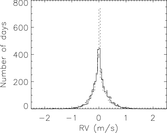
|
Figure 9: Histogram of RV (m/s) for spots+plages (solid line), spots (dotted line), and plages (dashed line), for the whole period. |
| Open with DEXTER | |
|
Figure 10: Upper panel: periodograms for the spot+plage RV for the whole serie. The horizontal dotted line show the level for a false-alarm probability of 1%. Lower panel: same for the total RV, i.e. taking the inhibition of the convective blueshift into account. |
| Open with DEXTER | |
|
Figure 11: Histogram of RV (m/s) for convection, for the whole period (solid line), low activity period (dotted line), and high activity period (dashed line). |
| Open with DEXTER | |
3.1.3 The total RV variations
Finally, we consider the total signal as shown in Fig. 7. The corresponding rms and maximum amplitude (peak-to-peak) are shown in Table 2, for the whole period, as well as the low and high activity periods. For the whole period, we reach an rms of 2.4 m/s, with a peak-to-peak amplitude above 11 m/s, clearly dominated by the convection signal. The amplitude is significantly lower during the low activity period, but can still reach peak-to-peak amplitudes of 2 m/s with a rms around 0.4-0.5 m/s.
Figure 10 shows the periodogram for the total RV signal over the whole period. The convection RV, which dominates the total signal, emphasizes the rotation period, however, because the sign is always the same. For the same reason, the long time-scale features are also emphasized. As the rotation period is often not known precisely, any more than the zero on the RV curves, such a difference between the two kinds of contributions may be difficult to separate.
3.2 Comparison with observed solar RV
There are no observations of the solar RV during the period covering our data set (cycle 23) that we are aware of. We therefore considered three previous studies covering either cycle 21 or 22. We have already compared the RV signal caused by spots in Paper I. It was not possible to use these observations to validate our simulation. By including plages it may be possible to make a more precise comparison, however.
McMillan et al. (1993) measured the
solar RV using the moon light observed in the violet part of the
spectrum. They have determined an upper limit for intrinsic solar
variations of ![]() 4 m/s,
during cycle 22 essentially (1987-1992). This is less than our
total RV variation. However, it is quite compatible with our rms RV for
the spots and plages only (0.33 m/s), as well as our maximum
peak-to-peak amplitude (2.4 m/s), even taking the slightly larger
contrasts in the violet into account. In the wavelength domain they
used, there is a very large proportion of deep lines, but as shown by Gray (2009),
these are the lines that have the lower convective blueshift, so it is
possible that their small RV comes from their being predominantly
sensitive to the spot+plage RV.
4 m/s,
during cycle 22 essentially (1987-1992). This is less than our
total RV variation. However, it is quite compatible with our rms RV for
the spots and plages only (0.33 m/s), as well as our maximum
peak-to-peak amplitude (2.4 m/s), even taking the slightly larger
contrasts in the violet into account. In the wavelength domain they
used, there is a very large proportion of deep lines, but as shown by Gray (2009),
these are the lines that have the lower convective blueshift, so it is
possible that their small RV comes from their being predominantly
sensitive to the spot+plage RV.
During a similar period (1983-1992), Deming & Plymate (1994) measured the solar RV in the 2.3 ![]() m
domain. They find a long-term variation with a peak-to-peak amplitude
of about 30 m/s, and a large dispersion on short time scales
(10-20 m/s). Considering that cycle 22 was more active than
cycle 23 by about 30%, we would expect long-term variations
of about 11 m/s, i.e. 3 times less than their observation. It
is quite possible that, in the wavelength domain they consider, the
convective blueshift is much more pronounced, but there has been no
such study that we are aware of to confirm that possibility. Their
short-term variations are also significantly greater than our results
for spots and plages, especially considering the reduced contrast
expected at 2.3
m
domain. They find a long-term variation with a peak-to-peak amplitude
of about 30 m/s, and a large dispersion on short time scales
(10-20 m/s). Considering that cycle 22 was more active than
cycle 23 by about 30%, we would expect long-term variations
of about 11 m/s, i.e. 3 times less than their observation. It
is quite possible that, in the wavelength domain they consider, the
convective blueshift is much more pronounced, but there has been no
such study that we are aware of to confirm that possibility. Their
short-term variations are also significantly greater than our results
for spots and plages, especially considering the reduced contrast
expected at 2.3 ![]() m.
m.
Finally, Jimenez et al. (1986) measured the solar RV in the potassium line at 769.9 nm (Brookes et al. 1978) during cycle 21 (1976-1984). On long time scales, they find a peak-to-peak amplitude of 30 m/s, which is compatible with that of Deming & Plymate (1994) and also 3 times larger than our convective signal. Their short time-scale variations can reach 20 m/s during cycle maximum, and are therefore also significantly more than our results.
Table 1: RV rms (in m/s) for specific components.
Table 2: RV rms and peak-to-peak amplitude (in m/s) and relative rms photometry for the three periods.
3.3 Discussion on the convection RV amplitude
3.3.1 Impact of the convective blueshift amplitude
We computed the convective RV variations on a short period (60 days) when using a ![]() from 50 m/s to 300 m/s. It appears that both the RV and BVS amplitudes vary linearly with
from 50 m/s to 300 m/s. It appears that both the RV and BVS amplitudes vary linearly with ![]() .
This means that it is easy to extrapolate to different convection conditions from our results.
.
This means that it is easy to extrapolate to different convection conditions from our results.
3.3.2 Impact of the areas cancelling the convective blueshift
As pointed out in Sect. 2.3.2, the reduction of the convective blueshift in the network structures outside active regions is more uncertain than in plages. We therefore recompute the convection RV while selecting structures (plages) only above 100 ppm. This corresponds to structures above 305 Mm2. We recall that the convective RV is correlated very well to the filling factor, and therefore we find results that are consistent with the relative contribution of these structures over the solar cycle. As shown by Meunier (2003), all structures including the smallest one (at the MDI spatial resolution) are correlated with the solar cycle, and the amplitude of variation decreases when the size decreases. Here, we find that these structures contribute to 35% of the rms RV during the low activity period, and to 55 % during the high activity period.
For comparison, the same large structures contribute in a larger proportion to the plage (photometric) RV: 68% during the low activity period and 83% during the high activity period. The reason is that, in that case, because similar structures on both side of the central meridian cancel each other and because small structures are more numerous and more homogeneously distributed over the solar surface, small structures contribute less than large structures, relative to their contribution to the filling factor. For convection however, all contributions add up, so they are directly related to the filling factor.
We also find that very small structures, for example those smaller than 80 Mm2 (typical network structures for Wang 1988), should contribute to 30% of the filling factor at cycle maximum and 70% at cycle minimum. When considering structures only above that size, we find that the plage RV has almost the same rms as before (0.29 m/s instead of 0.31 m/s, confirming the insignificant contribution of the smallest structures to the plage signal), but the rms of the convective RV is about 2 m/s instead of 2.5 m/s, so that these same small structures significantly contribute to that signal. As pointed out above, this only estimates the various contributions, but the exact attenuation of the convective blueshift in these regions is not well-known, even if we know that the granulation associated to them is abnormal.
Finally, the conservative threshold we have used to extract plage and network structures from MDI magnetograms implies that we are missing a significant part of the flux (e.g. Krivova & Solanki 2004) in very quiet regions, which may also be associated to a small attenuation of the convective blueshift, with a badly defined level. Therefore it is likely that our RV signal slightly underestimates the exact value.
In conclusion, considering plages above 100 ppm only provides a conservative lower limit for the convection contribution, i.e. about half the total signal during cycle maximum and about a third during the minimum.
3.3.3 Impact of the method
To separate the photometric contribution and the RV due to the
reduction of the convective blueshift in plages, we computed these two
contributions separately. We also computed the RV signal on a short
time series for plages that take both effects into account
simultaneously; i.e., we consider a plage contribution shifted by ![]() and with the usual plage contrast in temperature. We want to compare the resulting RV: RV
and with the usual plage contrast in temperature. We want to compare the resulting RV: RV
![]() with the sum of the plage and convection RV computed before RV
with the sum of the plage and convection RV computed before RV
![]() .
The difference between the two presents an rms of 0.04 m/s, which
is one order of magnitude smaller than the plage RV for that period
(about 0.4 m/s) and of course much smaller than the convection
contribution. RV
.
The difference between the two presents an rms of 0.04 m/s, which
is one order of magnitude smaller than the plage RV for that period
(about 0.4 m/s) and of course much smaller than the convection
contribution. RV
![]() and RV
and RV
![]() are
very well correlated (correlation of 0.97). There is however a
systematic offset of 0.23 m/s between the two, with RV
are
very well correlated (correlation of 0.97). There is however a
systematic offset of 0.23 m/s between the two, with RV
![]() larger than RV
larger than RV
![]() .
This value is, however, still smaller than the average RV
.
This value is, however, still smaller than the average RV
![]() (5.8 m/s). We conclude that our approach leads to the correct amplitude and variability of both contributions.
(5.8 m/s). We conclude that our approach leads to the correct amplitude and variability of both contributions.
4 Search for correlations of the radial velocity signal with other observables
4.1 Total solar irradiance
|
Figure 12: Total RV (m/s) versus the observed TSI (W/m2) for the whole data set (dots), for the low activity period (yellow triangles) and for the high activity period (pink squares). |
| Open with DEXTER | |
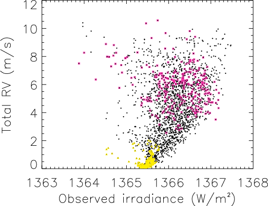
We compared the obtained RV with the observed TSI over the period 1996-2003. As photometry is often used as an activity criteria, it is important to check how the RV related to activity correlates with the TSI. There is no correlation between the RV due to spots and plages and the TSI. Low TSI values tend to correspond to periods with a small rms in RV, as already pointed out by Kürster et al. (2003). When considering the total RV (Fig. 12), there is a small correlation between the RV and TSI over the whole period (correlation of 0.40), although this correlation tends to disappear when considering shorter periods.
4.2 Ca index
|
Figure 13: Total RV (m/s) versus the Ca index for the whole data set (dots), for the low activity period (yellow triangles) and for the high activity period (pink squares). |
| Open with DEXTER | |
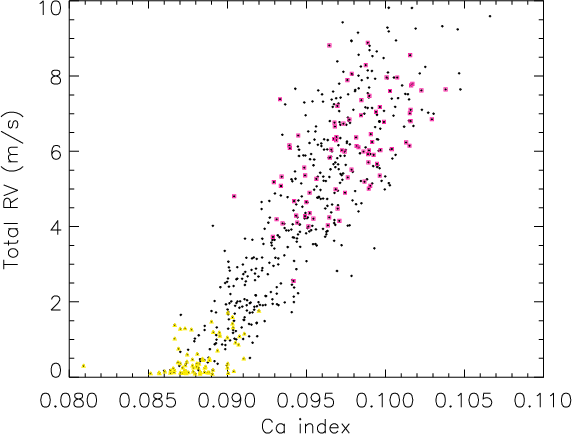
Another commonly used indicator of stellar activity is the Ca index. It is therefore useful to study the correlation between this indicator and the observed RV. As in Paper I we use the Ca index provided by the Sacramento Peak Observatory, for the period 1996-2002. There is no correlation between the RV signal considering only spots and plages and the Ca index. However, as already noted in Paper I for spots, periods with a low Ca index correspond to a small RV dispersion, while periods with larger Ca index correspond to a larger RV dispersion. When considering the total RV, i.e. taking the convection into account, over the whole period (Fig. 13), the correlation is strong (0.89). This is not surprising as the Ca index is related to plages, and the total RV is dominated by the convection signal (also related to plages, with no sign change).
![\begin{figure}
\par\includegraphics[width=7.8cm,clip]{13551fig14.ps}
\end{figure}](/articles/aa/full_html/2010/04/aa13551-09/img57.png)
|
Figure 14: Upper panel: periodogram of the spot+plage RV (m/s) added to the planet (see text) and a 1 cm/s noise, over the whole period. The sampling is the original one with 4-month gaps every year. The vertical dashed line indicates the planet orbital period. The dotted lines indicate the power corresponding to false alarm probabilities of 1% (upper line) and 10% (lower line). Lower panel: same for the total RV added to the planet (see text) and a 1 cm/s noise. |
| Open with DEXTER | |
5 Planets
To test the detectability of earth-type planets in the habitable zone, we have considered, as in Paper I, a 1
![]() planet orbiting at a 1.2 AU from the star on a circular orbit. The
RV amplitude of such a planet, for a system seen edge-on, is
0.08 m/s and its orbital period 480 days. We computed the
resulting RV signal for the whole data set, as well as for two periods
of low and high activity. The noise level is chosen to be 1 cm/s
(the goal for Espresso on the VLT, D'Odorico & the CODEX/ESPRESSO team 2007), 5 cm/s, and 10 cm/s (for Codex on the E-ELT, D'Odorico & the CODEX/ESPRESSO team 2007). Different temporal samplings were considered.
planet orbiting at a 1.2 AU from the star on a circular orbit. The
RV amplitude of such a planet, for a system seen edge-on, is
0.08 m/s and its orbital period 480 days. We computed the
resulting RV signal for the whole data set, as well as for two periods
of low and high activity. The noise level is chosen to be 1 cm/s
(the goal for Espresso on the VLT, D'Odorico & the CODEX/ESPRESSO team 2007), 5 cm/s, and 10 cm/s (for Codex on the E-ELT, D'Odorico & the CODEX/ESPRESSO team 2007). Different temporal samplings were considered.
5.1 Spot and plage RV variations
Figure 14 first shows the periodogram of the signal corresponding only to spots and plages, with a 1
![]() planet orbiting at a 1.2 AU and a 1 cm/s noise level. The
peak corresponding to the planet is highly significant (false alarm
probability below 10-12). The sampling is the original one with 4-month gaps every year to simulate a star that would not be visible at all times (
planet orbiting at a 1.2 AU and a 1 cm/s noise level. The
peak corresponding to the planet is highly significant (false alarm
probability below 10-12). The sampling is the original one with 4-month gaps every year to simulate a star that would not be visible at all times (
![]() )
as in Paper I. The same is true when considering only a few years
of low activity (extended to cover 790 days) or high activity (extended
to cover 2000 days). When degrading the temporal sampling down to
4 or 8 days, the amplitude of the planet peak decreases and
becomes barely significant, especially on the shorter periods, as in
Paper I.
)
as in Paper I. The same is true when considering only a few years
of low activity (extended to cover 790 days) or high activity (extended
to cover 2000 days). When degrading the temporal sampling down to
4 or 8 days, the amplitude of the planet peak decreases and
becomes barely significant, especially on the shorter periods, as in
Paper I.
5.2 Total RV variations
When considering the total RV (including the convection contribution), again with the
1
![]() planet orbiting at a 1.2 AU, a 1 cm/s noise level and a 4-month gap every year, Fig. 14
shows that the peak corresponding to the planet is not significant. It
is also adjacent to larger peaks at nearby periods. This is due to the
fact that convection dominates the spot+plage contribution, the noise,
and the planet, so that the total RV shows a long-term variability
related to the solar cycle, including on the scale of the year or a few
years, hence the adjacent peaks (see for example Fig. 10).
planet orbiting at a 1.2 AU, a 1 cm/s noise level and a 4-month gap every year, Fig. 14
shows that the peak corresponding to the planet is not significant. It
is also adjacent to larger peaks at nearby periods. This is due to the
fact that convection dominates the spot+plage contribution, the noise,
and the planet, so that the total RV shows a long-term variability
related to the solar cycle, including on the scale of the year or a few
years, hence the adjacent peaks (see for example Fig. 10).
If we decrease the amplitude of the convection contribution by just a
factor two (see Sect. 3.3.2), the planet peak has a false alarm
probabiblity of 18%; for a factor 5 it becomes
![]() .
The latter is very significant, but it is still adjacent to nearby
peaks that are as significant, therefore it would be very difficult to
identify it as caused by a planet. Increasing the noise level or
degrading the temporal sampling does not change the nature of the
problem. In conclusion, we would need to decrease the convection
contribution by one order of magnitude to be able to identify the
planet signal, even when using the best sampling.
.
The latter is very significant, but it is still adjacent to nearby
peaks that are as significant, therefore it would be very difficult to
identify it as caused by a planet. Increasing the noise level or
degrading the temporal sampling does not change the nature of the
problem. In conclusion, we would need to decrease the convection
contribution by one order of magnitude to be able to identify the
planet signal, even when using the best sampling.
6 Conclusion
We computed the expected solar RV variations caused by the photometric contribution of spots, as well as the contributions of plages through their photometry and the suppression of the convective blueshift between 1996 and 2007. The Sun was considered to be seen edge-on and observed in conditions similar to HARPS (spectral coverage and resolution). This work complements Paper I, which only considered the spot contribution. Our simulation reproduces the observed photometry, so we are confident that their relative contributions are correct. Our approach takes the complex activity pattern observed on the Sun into account. Even if the full characterization of such a complex pattern is currently beyond reach for other stars, precise photometric observations by COROT shows that solar-like stars can exhibit several short-lived spots at the same time (for example Mosser et al. 2009) or show a complex pattern between spots and plages (e.g. Lanza et al. 2009, for a young solar-like star). We obtain the main following results.
The photometric contributions of spots and plages only partially compensate for each other, so that the sum of these two signals is not very different from the spot signal. The shape of the RV distribution is not Gaussian and may provide information on the shape of the cycle, which may be a useful diagnosis tool in the future.
The plage contribution due to the convective blueshift suppression dominates the total signal. Unlike the previous one, the sign is always the same (a redshift when activity is present), i.e. is additive, and its long-term amplitude is about 8 m/s. The short time-scale RV rms is close to the m/s (and down to 0.4 m/s during the low activity period). Finally, we point out that this contribution is very line-dependent, as shown by Gray (2009), and therefore a precise computation must be made depending on the spectral range considered. If many lines are available, it should be possible in principle to compare the RV series computed using the strong and weak lines separately in order to identify the origin of the variation.
The comparison with observations of the solar RV is not easy, because of different temporal coverages and wavelength domains. The photometric signal should be sensitive to the wavelength domain because the contrast (assuming a black body) is lower in the red than in the violet part of the spectrum. On the other hand, the convective blueshift is very line-sensitive. Here we have estimated the contribution when considering most lines of the visible spectrum. On the other hand, all solar RV observations have focused on a single line or a restricted part of the spectrum, for which this convective blueshift might be very different and, unfortunately, has been poorly studied.
The RV is not correlated well with the total solar irradiance. Therefore a lack of correlation between observed RV and photometry should not lead to the conclusion that the observed RV cannot be due to activity. This is true for both the photometric contribution of spots and plages to the RV and for the convection signal. On the other hand, when the total RV is dominated by the convection signal, we expect from the present results a strong correlation with the Ca index. It is also dependent on the variability of the Ca index. The correlation remains very small, however, when only considering the photometric contribution of spots and plages to the RV.
We also tested the influence of activity and noise on the detection of an earth-like planet at 1.2 AU on a circular orbit. When considering only the photometric contribution of the spots and plages, the results are similar to that of Paper I. A good temporal sampling is necessary to detect the planet. On the other hand, when also taking the convection into account, the activity-related RVs completely dominate the signal at a level of about 8 m/s, and it seems impossible to detect the planet. Because there are other significant peaks in the same range of periods, the convection signal would need to be at least one order of magnitude weaker to make the identification of the planet peak possible, otherwise the adjacent peaks would still be of similar amplitude.
In conclusion, the photometric contribution to RV of both spots and plages at a level comparable to the Sun should not prevent detection of earth-like planets in the habitable zone around solar-like stars, providing a very good temporal sampling (better than 8 days and over a long monitoring period) and a good signal-to-noise ratio. On the other hand, the attenuation of the convective blueshift due to active regions, at the same level, seems to make it impossible to detect such a planet in similar conditions, as the orbital period is in the same range as the long-term strong activity signal. However, the properties of this contribution are such that some diagnosis may be established more easily than with the photometric contributions.
- The convective blueshift presents a strong spectral sensitivity, so
that using two masks (of respectively deep and weak lines) should lead
to significantly different RV variations. For example, for a
 of 200 m/s over all lines, we find 455 m/s for lines with
depths between 0.5 and 0.95 (weak lines) and 155 m/s for
lines with depths below 0.5 (strong lines), i.e. an expected
factor 2.7 between two such RV series.
of 200 m/s over all lines, we find 455 m/s for lines with
depths between 0.5 and 0.95 (weak lines) and 155 m/s for
lines with depths below 0.5 (strong lines), i.e. an expected
factor 2.7 between two such RV series.
- The correlation with the Ca index is very strong. Such a correlation could be used to correct long-term RV variations, as done by Saar & Fischer (2000).
- The BVS remains to be studied in detail, but we can expect it to be of large amplitude given the impact of that contribution on the lines, allowing it to be above the noise of future instruments. This will have to be confirmed using a realistic modelization of the line distortion when taking the convective blueshift into account.
The sunspot data have been provided by USAF/NOAA. SOHO is a mission of international cooperation between the European Space Agency (ESA) and NASA. The solar spectra were retrieved from the INSU/CNRS database BASS2000. The irradiance data set (version #25) were provided by PMOD/WRC, Davos, Switzerland, and we acknowledge unpublished data from the VIRGO experiment on the cooperative ESA/NASA mission SOHO. We acknowledge the Sacramento Peak Observatory of the U.S. Air Force Philips Laboratory for providing the Ca index. We acknowledge financial support from the French Programme National de Planétologie ( PNP, INSU). We also acknowledge support from the French National Research Agency (ANR) through project grant NT05-4_44463. We thank the referee, S. Solanki, for his useful comments on this paper.
References
- Balmaceda, L. A., Solanki, S. K., Krivova, N. A., & Foster, S. 2009, J. Geophys. Res. (Space Physics), 114, 7104 [Google Scholar]
- Brandt, P. N., & Solanki, S. K. 1990, A&A, 231, 221 [NASA ADS] [Google Scholar]
- Brookes, J. R., Isaak, G. R., & van der Raay, H. B. 1978, MNRAS, 185, 1 [NASA ADS] [Google Scholar]
- Cavallini, F., Ceppatelli, G., & Righini, A. 1985, A&A, 143, 116 [NASA ADS] [Google Scholar]
- Chapman, G. A., Cookson, A. M., & Dobias, J. J. 1994, ApJ, 432, 403 [NASA ADS] [CrossRef] [Google Scholar]
- Chapman, G. A., Cookson, A. M., Dobias, J. J., & Walton, S. R. 2001, ApJ, 555, 462 [NASA ADS] [CrossRef] [Google Scholar]
- Deming, D., & Plymate, C. 1994, ApJ, 426, 382 [Google Scholar]
- Desort, M., Lagrange, A.-M., Galland, F., Udry, S., & Mayor, M. 2007, A&A, 473, 983 [NASA ADS] [CrossRef] [EDP Sciences] [Google Scholar]
- D'Odorico, V., & the CODEX/ESPRESSO team 2007, Mem. Soc. Astron. Ital., 78, 712 [Google Scholar]
- Dravins, D. 1982, ARA&A, 20, 61 [NASA ADS] [CrossRef] [Google Scholar]
- Dravins, D. 1999, in ASP Conf. Ser. 185, IAU Coll., 170, Precise Stellar Radial Velocities, ed. J. B. Hearnshaw, & C. D. Scarfe, 268 [Google Scholar]
- Dravins, D., Lindegren, L., & Nordlund, A. 1981, A&A, 96, 345 [NASA ADS] [Google Scholar]
- Ermolli, I., Criscuoli, S., Centrone, M., Giorgi, F., & Penza, V. 2007, A&A, 465, 305 [NASA ADS] [CrossRef] [EDP Sciences] [Google Scholar]
- Fligge, M., Solanki, S. K., & Unruh, Y. C. 2000, A&A, 353, 380 [NASA ADS] [Google Scholar]
- Fligge, M., Solanki, S. K., Unruh, Y. C., Froehlich, C., & Wehrli, C. 1998, A&A, 335, 709 [NASA ADS] [Google Scholar]
- Foukal, P., Harvey, K., & Hill, F. 1991, ApJ, 383, L89 [NASA ADS] [CrossRef] [Google Scholar]
- Frazier, E. N. 1971, Sol. Phys., 21, 42 [NASA ADS] [CrossRef] [Google Scholar]
- Fröhlich, C. 2009, A&A, 501, L27 [NASA ADS] [CrossRef] [EDP Sciences] [Google Scholar]
- Fröhlich, C., & Lean, J. 1998, Geophys. Res. Lett., 25, 4377 [NASA ADS] [CrossRef] [Google Scholar]
- Galland, F., Lagrange, A.-M., Udry, S., et al. 2005, A&A, 443, 337 [NASA ADS] [CrossRef] [EDP Sciences] [Google Scholar]
- Gondoin, P. 2008, A&A, 478, 883 [NASA ADS] [CrossRef] [EDP Sciences] [Google Scholar]
- Gray, D. F. 2009, ApJ, 697, 1032 [NASA ADS] [CrossRef] [Google Scholar]
- Guenther, E., & Mattig, W. 1991, A&A, 243, 244 [NASA ADS] [Google Scholar]
- Hanslmeier, A., & Mattig, W. 1990, Ap&SS, 170, 51 [NASA ADS] [CrossRef] [Google Scholar]
- Hanslmeier, A., Nesis, A., & Mattig, W. 1991, A&A, 251, 307 [NASA ADS] [Google Scholar]
- Hanslmeier, A., Nesis, A., & Mattig, W. 1994, A&A, 288, 960 [NASA ADS] [Google Scholar]
- Hatzes, A. P. 2002, Astron. Nachr., 323, 392 [NASA ADS] [CrossRef] [Google Scholar]
- Immerschitt, S., & Schroeter, E. H. 1989, A&A, 208, 307 [NASA ADS] [Google Scholar]
- Jimenez, A., Palle, P. L., Regulo, C., Roca Cortes, T., & Isaak, G. R. 1986, Adv. Space Res., 6, 89 [NASA ADS] [CrossRef] [PubMed] [Google Scholar]
- Krivova, N. A., & Solanki, S. K. 2004, A&A, 417, 1125 [NASA ADS] [CrossRef] [EDP Sciences] [Google Scholar]
- Krivova, N. A., Solanki, S. K., Fligge, M., & Unruh, Y. C. 2003, A&A, 399, L1 [NASA ADS] [CrossRef] [EDP Sciences] [Google Scholar]
- Kürster, M., Endl, M., Rouesnel, F., et al. 2003, A&A, 403, 1077 [NASA ADS] [CrossRef] [EDP Sciences] [Google Scholar]
- Lagrange, A. M., Desort, M., & Meunier, N. 2010, A&A, 512, A38 (Paper I) [NASA ADS] [CrossRef] [EDP Sciences] [Google Scholar]
- Lanza, A. F., Bonomo, A. S., & Rodonò, M. 2007, A&A, 464, 741 [NASA ADS] [CrossRef] [EDP Sciences] [Google Scholar]
- Lanza, A. F., Pagano, I., Leto, G., et al. 2009, A&A, 493, 193 [NASA ADS] [CrossRef] [EDP Sciences] [Google Scholar]
- Lanza, A. F., Rodonò, M., & Pagano, I. 2004, A&A, 425, 707 [NASA ADS] [CrossRef] [EDP Sciences] [Google Scholar]
- Lawrence, J. K. 1988, Sol. Phys., 116, 17 [NASA ADS] [CrossRef] [Google Scholar]
- Livingston, W., Wallace, L., Huang, Y., & Moise, E. 1999, in High Resolution Solar Physics: Theory, Observations, and Techniques, ed. T. R. Rimmele, K. S. Balasubramaniam, & R. R. Radick, ASP Conf. Ser., 183, 494 [Google Scholar]
- Lockwood, G. W., Skiff, B. A., Henry, G. W., et al. 2007, ApJS, 171, 260 [NASA ADS] [CrossRef] [Google Scholar]
- Marquez, I., Bonet, J. A., & Vazquez, M. 1996, A&A, 306, 305 [NASA ADS] [Google Scholar]
- Martinez Pillet, V., Lites, B. W., & Skumanich, A. 1997, ApJ, 474, 810 [NASA ADS] [CrossRef] [Google Scholar]
- McMillan, R. S., Moore, T. L., Perry, M. L., & Smith, P. H. 1993, ApJ, 403, 801 [NASA ADS] [CrossRef] [Google Scholar]
- Meunier, N. 2003, A&A, 405, 1107 [NASA ADS] [CrossRef] [EDP Sciences] [Google Scholar]
- Morinaga, S., Sakurai, T., Ichimoto, K., et al. 2008, A&A, 481, L29 [NASA ADS] [CrossRef] [EDP Sciences] [Google Scholar]
- Mosser, B., Baudin, F., Lanza, A. F., et al. 2009, A&A, 506, 245 [NASA ADS] [CrossRef] [EDP Sciences] [Google Scholar]
- Muller, R., Hulot, J. C., & Roudier, T. 1989, Sol. Phys., 119, 229 [NASA ADS] [CrossRef] [Google Scholar]
- Ortiz, A., Domingo, V., & Sanahuja, B. 2006, A&A, 452, 311 [NASA ADS] [CrossRef] [EDP Sciences] [Google Scholar]
- Ortiz, A., Solanki, S. K., Domingo, V., Fligge, M., & Sanahuja, B. 2002, A&A, 388, 1036 [NASA ADS] [CrossRef] [EDP Sciences] [Google Scholar]
- Saar, S. H. 2003, in ASP Conf. Ser., 294, Scientific Frontiers in Research on Extrasolar Planets, ed. D. Deming, & S. Seager, 65 [Google Scholar]
- Saar, S. H., & Donahue, R. A. 1997, ApJ, 485, 319 [NASA ADS] [CrossRef] [Google Scholar]
- Saar, S. H., & Fischer, D. 2000, ApJ, 534, L105 [NASA ADS] [CrossRef] [PubMed] [Google Scholar]
- Scherrer, P. H., Bogart, R. S., Bush, R. I., et al. 1995, Sol. Phys., 162, 129 [Google Scholar]
- Schmidt, W., Grossmann-Doerth, U., & Schroeter, E. H. 1988, A&A, 197, 306 [NASA ADS] [Google Scholar]
- Solanki, S. K. 1986, A&A, 168, 311 [NASA ADS] [Google Scholar]
- Title, A. M., Tarbell, T. D., & Topka, K. P. 1987, ApJ, 317, 892 [NASA ADS] [CrossRef] [Google Scholar]
- Unruh, Y. C., Solanki, S. K., & Fligge, M. 1999, A&A, 345, 635 [NASA ADS] [Google Scholar]
- Wang, H. 1988, Sol. Phys., 117, 343 [NASA ADS] [CrossRef] [Google Scholar]
- Worden, J. R., White, O. R., & Woods, T. N. 1998, ApJ, 496, 998 [Google Scholar]
Footnotes
- ... deficit
![[*]](/icons/foot_motif.png)
- With respect to the photospheric temperature of 5800 K.
- ... contrast
- Defined as
 ,
with
,
with
 the photospheric irradiance and
 the plage irradiance.
All Tables
Table 1: RV rms (in m/s) for specific components.
Table 2: RV rms and peak-to-peak amplitude (in m/s) and relative rms photometry for the three periods.
All Figures
|
|
Figure 1: Upper panel: MDI magnetogram for September 14, 2002 at 4:48 UT (left) and Meudon photospheric spectroheliogram at 6:41 UT (right). Lower panel: simulated map showing the plages derived from the magnetogram with a contrast increased by a factor 10 for clarity ( left) and the spots from the USAF/NOAA data set at 12:40 UT (right). |
| Open with DEXTER | |
| In the text | |
|
|
Figure 2: Upper panel: projected spot filling factor versus time, in ppm of the solar disk. Lower panel: same for plages. |
| Open with DEXTER | |
| In the text | |
|
|
Figure 3:
Upper panel: plage temperature excess versus |
| Open with DEXTER | |
| In the text | |
|
|
Figure 4:
Upper panel: spot temperature deficit versus the spot-surface
scaling factor for the explored range of scaling factors (see text for
details). For a given spot-surface scaling factor, the various points
correspond to different plage-surface scaling factors. Bottom panel: same for plages at |
| Open with DEXTER | |
| In the text | |
|
|
Figure 5: First panel: reconstructed spot contribution to irradiance. Second panel: reconstructed plage contribution to irradiance. Third panel: total reconstructed irradiance. Fourth panel: observed irradiance. |
| Open with DEXTER | |
| In the text | |
|
|
Figure 6: Total reconstructed irradiance versus the observed irradiance (W/m2). |
| Open with DEXTER | |
| In the text | |
|
|
Figure 7: Left column: RV (m/s) for spot signal, plage signal, convection signal, and total ( From top to bottom), for the whole data set. Middle column: same for the low activity period. Right column: same for the high activity period. |
| Open with DEXTER | |
| In the text | |
|
|
Figure 8: Upper panel: RV signal from spots (dotted line), plages (dashed line), and spots+plages (solid line) in m/s, for julian days 2 451 790-2 451 850, i.e. during the high activity period. Lower panel: same for spots+plages (dotted line), convection (dashed line), and total (solid line). |
| Open with DEXTER | |
| In the text | |
|
|
Figure 9: Histogram of RV (m/s) for spots+plages (solid line), spots (dotted line), and plages (dashed line), for the whole period. |
| Open with DEXTER | |
| In the text | |
|
|
Figure 10: Upper panel: periodograms for the spot+plage RV for the whole serie. The horizontal dotted line show the level for a false-alarm probability of 1%. Lower panel: same for the total RV, i.e. taking the inhibition of the convective blueshift into account. |
| Open with DEXTER | |
| In the text | |
|
|
Figure 11: Histogram of RV (m/s) for convection, for the whole period (solid line), low activity period (dotted line), and high activity period (dashed line). |
| Open with DEXTER | |
| In the text | |
|
|
Figure 12: Total RV (m/s) versus the observed TSI (W/m2) for the whole data set (dots), for the low activity period (yellow triangles) and for the high activity period (pink squares). |
| Open with DEXTER | |
| In the text | |
|
|
Figure 13: Total RV (m/s) versus the Ca index for the whole data set (dots), for the low activity period (yellow triangles) and for the high activity period (pink squares). |
| Open with DEXTER | |
| In the text | |
|
|
Figure 14: Upper panel: periodogram of the spot+plage RV (m/s) added to the planet (see text) and a 1 cm/s noise, over the whole period. The sampling is the original one with 4-month gaps every year. The vertical dashed line indicates the planet orbital period. The dotted lines indicate the power corresponding to false alarm probabilities of 1% (upper line) and 10% (lower line). Lower panel: same for the total RV added to the planet (see text) and a 1 cm/s noise. |
| Open with DEXTER | |
| In the text | |
Copyright ESO 2010
Current usage metrics show cumulative count of Article Views (full-text article views including HTML views, PDF and ePub downloads, according to the available data) and Abstracts Views on Vision4Press platform.
Data correspond to usage on the plateform after 2015. The current usage metrics is available 48-96 hours after online publication and is updated daily on week days.
Initial download of the metrics may take a while.