| Issue |
A&A
Volume 511, February 2010
|
|
|---|---|---|
| Article Number | A47 | |
| Number of page(s) | 12 | |
| Section | Stellar atmospheres | |
| DOI | https://doi.org/10.1051/0004-6361/200913693 | |
| Published online | 05 March 2010 | |
Lithium abundances of halo dwarfs based on excitation temperatures
II. Non-local thermodynamic equilibrium
A. Hosford1 - A. E. García Pérez1 - R. Collet2 - S. G. Ryan1 - J. E. Norris3 - K. A. Olive4
1 - Centre for Astrophysics Research, University of Hertfordshire,
College Lane, Hatfield, AL10 9AB, UK
2 - Max-Planck-Institut für Astrophysik, Postfach 1317, 85741 Garching
bei München, Germany
3 - Research School of Astronomy and Astrophysics, The Australian
National University, Mount Stromlo Observatory, Cotter Road, Weston,
ACT 2611, Australia
4 - William I. Fine Theoretical Physics Institute, School of Physics
and Astronomy, University of Minnesota, Minneapolis, MN 55455, USA
Received 18 November 2009 / Accepted 4 January 2010
Abstract
Context. The plateau in the abundance of 7Li
in metal-poor stars was initially interpreted as an observational
indicator of the primordial lithium abundance. However, this
observational value is in disagreement with that deduced from
calculations of Big Bang nucleosynthesis (BBN), when using the
Wilkinson microwave anisotropy probe (WMAP) baryon density
measurements. One of the most important factors in determining the
stellar lithium abundance is the effective temperature. In a previous
study by the authors, new effective temperatures (
![]() )
for sixteen metal-poor halo dwarfs were derived using a local
thermodynamic equilibrium (LTE) description of the formation of Fe
lines. This new
)
for sixteen metal-poor halo dwarfs were derived using a local
thermodynamic equilibrium (LTE) description of the formation of Fe
lines. This new ![]() scale reinforced the discrepancy.
scale reinforced the discrepancy.
Aims. For six of the stars from our previous study
we calculate revised temperatures using a non-local thermodynamic
equilibrium (NLTE) approach. These are then used to derive a new mean
primordial lithium abundance in an attempt to solve the lithium
discrepancy.
Methods. Using the code ![]() we calculate NLTE corrections to the LTE abundances for the Fe I
lines measured in the six stars, and determine new
we calculate NLTE corrections to the LTE abundances for the Fe I
lines measured in the six stars, and determine new ![]() 's. We keep
other physical parameters, i.e. log g, [Fe/H] and
's. We keep
other physical parameters, i.e. log g, [Fe/H] and ![]() ,
constant at the values calculated in Paper I. With the revised
,
constant at the values calculated in Paper I. With the revised
![]() scale we
derive new Li abundances. We compare the NLTE values of
scale we
derive new Li abundances. We compare the NLTE values of ![]() with the photometric temperatures of Ryan et al. (1999, ApJ,
523, 654), the infrared flux method (IRFM) temperatures of Meléndez
& Ramírez (2004, ApJ, 615, L33), and the Balmer line wing
temperatures of Asplund et al. (2006, ApJ, 644, 229).
with the photometric temperatures of Ryan et al. (1999, ApJ,
523, 654), the infrared flux method (IRFM) temperatures of Meléndez
& Ramírez (2004, ApJ, 615, L33), and the Balmer line wing
temperatures of Asplund et al. (2006, ApJ, 644, 229).
Results. We find that our temperatures are hotter
than both the Ryan et al. and Asplund et al.
temperatures by typically ![]() 110-160 K,
but are still cooler than the temperatures of Meléndez &
Ramírez by typically
110-160 K,
but are still cooler than the temperatures of Meléndez &
Ramírez by typically ![]() 190 K.
The temperatures imply a primordial Li abundance of 2.19 dex
or 2.21 dex, depending on the magnitude of collisions with
hydrogen in the calculations, still well below the value of
2.72 dex inferred from WMAP + BBN. We discuss the effects of
collisions on trends of 7Li abundances with
[Fe/H] and
190 K.
The temperatures imply a primordial Li abundance of 2.19 dex
or 2.21 dex, depending on the magnitude of collisions with
hydrogen in the calculations, still well below the value of
2.72 dex inferred from WMAP + BBN. We discuss the effects of
collisions on trends of 7Li abundances with
[Fe/H] and ![]() ,
as well as the NLTE effects on the determination of log g
through ionization equilibrium, which imply a collisional scaling
factor
,
as well as the NLTE effects on the determination of log g
through ionization equilibrium, which imply a collisional scaling
factor ![]() for collisions between Fe
for collisions between Fe
Conclusions. And H
atoms.
Key words: Galaxy: halo - early Universe - stars: abundances - stars: atmospheres - line: formation - radiative transfer
1 Introduction
Since its discovery by Spite
& Spite (1982), many studies of the plateau in
lithium in metal-poor dwarfs have been undertaken, e.g. Spite et al. (1996),
Ryan et al. (2000),
Meléndez & Ramírez
(2004), Bonifacio
et al. (2007) and Aoki
et al. (2009), confirming its existence. Most
studies find a comparable Li abundance (A(Li)![]()
![]() 2.0-2.1 dex)
yet discrepancies still exist, in particular the high value found by Meléndez & Ramírez (2004)
(A(Li) = 2.37 dex). However, the biggest
discrepancy comes from a comparison of the primordial abundances
inferred from observations and that derived from Big Bang
nucleosynthesis (BBN) with the WMAP constraint on the baryon density
fraction,
2.0-2.1 dex)
yet discrepancies still exist, in particular the high value found by Meléndez & Ramírez (2004)
(A(Li) = 2.37 dex). However, the biggest
discrepancy comes from a comparison of the primordial abundances
inferred from observations and that derived from Big Bang
nucleosynthesis (BBN) with the WMAP constraint on the baryon density
fraction, ![]() ,
which leads to A(Li) = 2.72 dex (Cyburt et al. 2008).
This is what has become known as the ``lithium problem''.
,
which leads to A(Li) = 2.72 dex (Cyburt et al. 2008).
This is what has become known as the ``lithium problem''.
Several possibilities have been proposed to explain this
discrepancy. Broadly these are: systematic errors in the derived
stellar Li abundances; errors in the BBN calculations due to
uncertainties in some of the relevant nuclear reaction rates; the
destruction of some of the BBN-produced Li prior to the formation of
the stars we have observed; the introduction of new physics that may
affect BBN (Jedamzik
& Pospelov 2009); or the removal of Li from the
photospheres of the stars through their lifetimes (see introduction to Hosford et al. 2009,
Paper I, for more details). The possible explanation under study in
this work is that of systematic errors in the effective temperature (
![]() )
scale for metal-poor stars. The effective temperature is the most
important atmospheric parameter affecting the determination of Li
abundances. This is due to the high sensitivity of A(Li)
to
)
scale for metal-poor stars. The effective temperature is the most
important atmospheric parameter affecting the determination of Li
abundances. This is due to the high sensitivity of A(Li)
to ![]() ,
with
,
with ![]() dex
per 100 K. One reason for the spread in the observed A(Li)
is the differences in the
dex
per 100 K. One reason for the spread in the observed A(Li)
is the differences in the ![]() scales used by different authors. For instance, Spite et al. (1996)
and Asplund et al.
(2006) derive a
scales used by different authors. For instance, Spite et al. (1996)
and Asplund et al.
(2006) derive a ![]() of 5540 K and 5753 K for the star HD 140283,
respectively. The scale of Meléndez
& Ramírez (2004) is on average
of 5540 K and 5753 K for the star HD 140283,
respectively. The scale of Meléndez
& Ramírez (2004) is on average ![]() 200 K
hotter than other works. This goes some way to explaining their higher A(Li);
other factors, such as the model atmospheres with convective
overshooting used in their work, may also contribute to the
discrepancy. It is important to confirm, or rule out, whether
systematic errors in
200 K
hotter than other works. This goes some way to explaining their higher A(Li);
other factors, such as the model atmospheres with convective
overshooting used in their work, may also contribute to the
discrepancy. It is important to confirm, or rule out, whether
systematic errors in ![]() are the cause of the Li problem, and in doing so address the need for
other possible explanations.
are the cause of the Li problem, and in doing so address the need for
other possible explanations.
In previous work (Hosford
et al. 2009, Paper I), we utilised the exponential
sensitivity in the Boltzmann distribution to ![]() ,
where
,
where ![]() is the excitation energy of the lower level of a transition. Using
this, we determined
is the excitation energy of the lower level of a transition. Using
this, we determined ![]() 's
for eighteen metal-poor stars close to the main-sequence turnoff. This
was done by nulling the dependence of A(Fe) on
's
for eighteen metal-poor stars close to the main-sequence turnoff. This
was done by nulling the dependence of A(Fe) on ![]() for approx 80-150 Fe I lines. Two
for approx 80-150 Fe I lines. Two ![]() scales were generated due to uncertainty in the evolutionary state of
some of the stars under study. It was found that our temperatures were
in good agreement with those derived by a Balmer line wing method by Asplund et al. (2006)
and those derived by photometric techniques by Ryan et al. (1999).
However, our
scales were generated due to uncertainty in the evolutionary state of
some of the stars under study. It was found that our temperatures were
in good agreement with those derived by a Balmer line wing method by Asplund et al. (2006)
and those derived by photometric techniques by Ryan et al. (1999).
However, our ![]() scale was on average
scale was on average ![]() 250 K
cooler than temperatures from the infrared flux method (IRFM) as
implemented by Meléndez
& Ramírez (2004). This is not the case for all work
done using the IRFM, the IRFM effective temperatures of Alonso et al. (1996)
are similar to ours, for stars we have in common.
250 K
cooler than temperatures from the infrared flux method (IRFM) as
implemented by Meléndez
& Ramírez (2004). This is not the case for all work
done using the IRFM, the IRFM effective temperatures of Alonso et al. (1996)
are similar to ours, for stars we have in common.
The derived mean abundances in Paper I were A(Li)
= 2.16 dex assuming main-sequence (MS) membership and A(Li)
= 2.10 dex assuming sub-giant branch (SGB) membership. For the
five stars that have a known evolutionary state, we calculated a mean A(Li)
= 2.18 dex. It is clear that these values are not high enough
to solve the lithium problem. However, the analysis of Hosford et al. (2009)
assumed that the spectrum was formed in local thermodynamic equilibrium
(LTE). This is a standard way of calculating spectra, but
oversimplifies the radiative transfer problem, and it was acknowledged
in Hosford et al.
(2009) that LTE simplification affect those results.
Consequently, although it was shown that, within the LTE framework,
systematic errors in the ![]() scale are not the cause of the disparity between spectroscopic and
BBN+WMAP values for the primordial Li, we also need to assess the
impact of non-local thermodynamic equilibrium (NLTE) on the
determination of stars effective temperatures. That is the aim of the
current work.
scale are not the cause of the disparity between spectroscopic and
BBN+WMAP values for the primordial Li, we also need to assess the
impact of non-local thermodynamic equilibrium (NLTE) on the
determination of stars effective temperatures. That is the aim of the
current work.
This work is not intended to be a full dissection of the
methods of NLTE, but rather an application of those more complex (and
possibly more accurate) methods to derive a new ![]() scale and to assess their impact on the lithium problem. However, to do
this we need to delve, with some depth, into the processes of NLTE line
formation, which we do in Sect. 2. This will give some
understanding of the complexities and uncertainties that are involved
and give the opportunity to make some generalisations on the important
aspects that need to be addressed. In Sects. 3-5 we detail our
calculations and results, and discuss these further in
Sect. 6.
scale and to assess their impact on the lithium problem. However, to do
this we need to delve, with some depth, into the processes of NLTE line
formation, which we do in Sect. 2. This will give some
understanding of the complexities and uncertainties that are involved
and give the opportunity to make some generalisations on the important
aspects that need to be addressed. In Sects. 3-5 we detail our
calculations and results, and discuss these further in
Sect. 6.
2 NLTE framework
2.1 The necessity for NLTE
With the availability of high quality spectra, the problem of
calculating accurate chemical abundances often comes down to a better
understanding of the line formation process. This is of particular
importance to this work as the calculation of accurate level
populations of the Fe I atom and source
functions at the wavelengths of the Fe transitions is crucial to
determining ![]() from lines of different
from lines of different ![]() .
In LTE calculations, the level populations follow the Boltzmann and
Saha distributions. These assume that the levels are populated, or
depopulated, by collisional and/or radiative processes, that are
characterised by the local kinetic temperature. In the deep layers of
the atmosphere, at
.
In LTE calculations, the level populations follow the Boltzmann and
Saha distributions. These assume that the levels are populated, or
depopulated, by collisional and/or radiative processes, that are
characterised by the local kinetic temperature. In the deep layers of
the atmosphere, at ![]() ,
where
,
where ![]() is the optical depth at 5000 Å, LTE is a reasonable
assumption. However, it tends to break down at optical depths
is the optical depth at 5000 Å, LTE is a reasonable
assumption. However, it tends to break down at optical depths ![]() ,
i.e. through most of the line forming region of the photosphere.
Therefore neglecting deviations of the level populations from LTE could
lead to errors in the
,
i.e. through most of the line forming region of the photosphere.
Therefore neglecting deviations of the level populations from LTE could
lead to errors in the ![]() derived by excitation dependence. Furthermore, in NLTE calculations, it
is not only the level populations that differ from the LTE case. The
radiative transitions of the atom must be explicitly considered. The
fact that the radiation field is no longer described by a Planck
function, and certainly not a Planck function calculated for the local
temperature, results in further changes of the spectrum relative to the
LTE case. This last effect is very important in metal-poor stars, where
the reduced opacity/increased transparency of the atmosphere exposes
shallow, cooler layers to the UV-rich spectrum coming from the deeper,
hotter layers (Asplund
et al. 1999).
derived by excitation dependence. Furthermore, in NLTE calculations, it
is not only the level populations that differ from the LTE case. The
radiative transitions of the atom must be explicitly considered. The
fact that the radiation field is no longer described by a Planck
function, and certainly not a Planck function calculated for the local
temperature, results in further changes of the spectrum relative to the
LTE case. This last effect is very important in metal-poor stars, where
the reduced opacity/increased transparency of the atmosphere exposes
shallow, cooler layers to the UV-rich spectrum coming from the deeper,
hotter layers (Asplund
et al. 1999).
For Fe in particular, different studies have come to different
conclusions as to the magnitude of the NLTE corrections. Thévenin & Idiart (1999)
found that there can be corrections of up to 0.35 dex on Fe I
abundances for main-sequence stars at [Fe/H] ![]() ,
and suggest that all work done on metal-poor stars should be carried
out using NLTE methods. Gratton
et al. (1999), however, find negligible corrections
to Fe I abundances and see this as
validation that LTE assumptions still hold when studying this type of
star. In contrast, work by Shchukina
et al. (2005) find higher correction values of
,
and suggest that all work done on metal-poor stars should be carried
out using NLTE methods. Gratton
et al. (1999), however, find negligible corrections
to Fe I abundances and see this as
validation that LTE assumptions still hold when studying this type of
star. In contrast, work by Shchukina
et al. (2005) find higher correction values of ![]() 0.9 dex
and
0.9 dex
and ![]() 0.6 dex,
depending on whether 3D or 1D atmospheres are used. The difference in
their conclusions is driven principally by the different relative
importance of collisional and radiative transitions in their
calculations. Gratton
et al. (1999) have relatively stronger collisional
transitions, and as a result find smaller deviations from LTE. Shchukina et al. (2005)
include no collisions with neutral hydrogen. We return to this
important point below, but for now it illustrates that much work still
needs to be done in this field before we can be certain of the impact
of NLTE.
0.6 dex,
depending on whether 3D or 1D atmospheres are used. The difference in
their conclusions is driven principally by the different relative
importance of collisional and radiative transitions in their
calculations. Gratton
et al. (1999) have relatively stronger collisional
transitions, and as a result find smaller deviations from LTE. Shchukina et al. (2005)
include no collisions with neutral hydrogen. We return to this
important point below, but for now it illustrates that much work still
needs to be done in this field before we can be certain of the impact
of NLTE.
2.2 The coupling of the radiation field and level populations
Many factors have to be taken into account when computing radiative transfer in NLTE. This leads to a complicated situation where, for example, we have to solve population equations and radiative transfer equations simultaneously. This is due to the level populations and the radiation field being coupled, a fact ignored in LTE calculations. There are large uncertainties in NLTE calculations because of the lack of complete information on the rates of collisional and radiative transitions between energy levels for a given element in all its important ionization states. This is especially true for larger atoms which have a greater number of energy levels, as is the case for Fe.
To solve NLTE problems, a system of rate equations is needed
that describes fully the populations of each level within the atom
under study. Statistical equilibrium is invoked, i.e. the radiation
fields and the level populations are constant with time. The
formulation of the problem is well described in Mihalas (1978), from which the
following equations are taken. The population of level i
is the sum of all the processes that populate the level minus the
processes that depopulate it, such that:
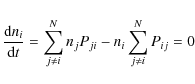
|
(1) |
where
|
(2) |
where

|
(3) |
where
![\begin{displaymath}S^l_\nu = \left( {\frac{{2h\nu ^3 }}{{c^2 }}} \right)\left[ {...
...( {\frac{{n_i g_j }}{{n_j g_i }}} \right) - 1} \right]^{ - 1}
\end{displaymath}](/articles/aa/full_html/2010/03/aa13693-09/img49.png)
|
(4) |
here h is Planck's constant, c is the speed of light,
2.3 Transition rates
For the calculation of the level populations, through Eq. (1), radiative and collisional rates are required.For the radiative rates, the bound-bound transition
probabilities and photoionization cross sections are needed for all
levels of the atom in all significant ionization states. Two of the
larger projects providing values for these are the Opacity Project (Seaton 1987) and the IRON
project (Bautista 1997).
For Fe, the Opacity Project finds typically a >10 ![]() uncertainty for their photoionization data (Seaton
et al. 1994). The Bautista photoionization values,
which are larger than those previously used, lead to increased
photoionization rates (Asplund 2005)
and hence to lower abundances as overionization becomes more efficient.
uncertainty for their photoionization data (Seaton
et al. 1994). The Bautista photoionization values,
which are larger than those previously used, lead to increased
photoionization rates (Asplund 2005)
and hence to lower abundances as overionization becomes more efficient.
For the collisional data, large uncertainties still exist. The two main types of collisions that affect the line profile are those with electrons and neutral hydrogen. Coupling of all levels in the Fe model atom occurs due to these types of collisions, especially in the atmospheres of cool stars where electrons and neutral H are believed to be the dominant perturbers. A simple calculation, like that in Asplund (2005), shows that H I collisions dominate over electron collisions in thermalizing processes in metal-poor stars and are therefore important in calculations of line profiles. For collisions with neutral hydrogen, the approximate formulation of Drawin (1969,1968) is used as implemented by Steenbock & Holweger (1984). However, through laboratory testing and quantum calculations of collisions with atoms such as Li and Na, it has been shown that Drawin's formula does not produce the correct order of magnitude result for H I collisional cross-sections. In some cases, where comparisons with experimental data or theoretical results can be made, the Drawin recipe overestimates the cross-sections by one to six orders of magnitude (e.g. Fleck et al. 1991; Barklem et al. 2003). Corrections to the Drawin cross-sections are suggested by Lambert (1993) to compensate for these differences.
Due to the uncertainties in the magnitude of the H collisions,
the Drawin cross-sections are scaled with a factor ![]() .
There are different schools of thought on how to deal with this
parameter. Collet
et al. (2005) treat it as a free parameter in their
work, adopting values of
.
There are different schools of thought on how to deal with this
parameter. Collet
et al. (2005) treat it as a free parameter in their
work, adopting values of ![]() and 1 and test the effect this has on their results. Higher values of
and 1 and test the effect this has on their results. Higher values of ![]() correspond to more collisions and hence more LTE-like conditions. Their
main aim, however, was to test not the efficiency of H collisions but
the effects of line-blocking on the NLTE problem. Korn et al. (2003)
make it one of their aims to constrain
correspond to more collisions and hence more LTE-like conditions. Their
main aim, however, was to test not the efficiency of H collisions but
the effects of line-blocking on the NLTE problem. Korn et al. (2003)
make it one of their aims to constrain ![]() .
To do this, they ensure ionization equilibrium between Fe I
and Fe II using the log g
derived from HIPPARCOS parallax and
.
To do this, they ensure ionization equilibrium between Fe I
and Fe II using the log g
derived from HIPPARCOS parallax and ![]() from H lines. In doing this, they find that a value of
from H lines. In doing this, they find that a value of ![]() holds for a group of local metal-poor stars. This apparently
contradicts the statement above that Drawin's formula overestimates the
cross-sections. Gratton
et al. (1999) use
holds for a group of local metal-poor stars. This apparently
contradicts the statement above that Drawin's formula overestimates the
cross-sections. Gratton
et al. (1999) use ![]() .
This value was constrained by increasing
.
This value was constrained by increasing ![]() until spectral features of several elements, i.e. Fe, O, Na and Mg, of
RR Lyrae stars all gave the same abundance. With such elevated
collisional rates, Gratton
et al. (1999) not surprisingly find results very
close to LTE, i.e. they find very small NLTE corrections.
until spectral features of several elements, i.e. Fe, O, Na and Mg, of
RR Lyrae stars all gave the same abundance. With such elevated
collisional rates, Gratton
et al. (1999) not surprisingly find results very
close to LTE, i.e. they find very small NLTE corrections.
Collisions with neutral hydrogen and electrons are important not only in coupling bound states to each other, but also in coupling the whole system to the continuum i.e. to the Fe II ground state (and potentially excited states). This is especially true when considering the high excitation levels. These levels are more readily collisionally ionised than lower levels, and are also coupled to each other by low energy (infrared) transitions, therefore thermalization of the levels occurs which drives the populations more towards LTE values. It is therefore important to have a model atom that includes as many of the higher terms of the atom as possible (Korn 2008), although it is not necessary to include all individual levels. We return to this point in Sect. 4. We describe the model atom and calculations next before moving on to the results.
2.4 The model Fe atom
The Fe model adopted for this work is that of Collet et al. (2005), which is an updated version of the model atom of Thévenin & Idiart (1999). The atom includes 334 levels of Fe I with the highest level at 6.91 eV. For comparison, the first ionization energy is 7.78 eV and the NIST database lists 493 Fe I levels. Many of the highest levels are not included in our model; due in part to computational limitations i.e. the more complicated the model, the greater the computer power and time needed to complete the computations, and because of lack of important information, e.g. photoionization cross sections. We report below on the effects the missing upper levels have on the corrections and try to quantify their importance in the NLTE calculations. The model also includes 189 levels of Fe II with the highest level at 16.5 eV, and the ground level of Fe III. For comparison, the second ionization energy is 16.5 eV, and the NIST database lists 578 Fe II levels. This model configuration leads to the possibility of 3466 bound-bound radiative transitions in the Fe I system, 3440 in the Fe II system, and 523 bound-free transitions. We run the calculations with the whole model, but present results only for the lines that are measured in our program stars.
Oscillator strengths for the Fe I lines are taken from Nave et al. (1994) and Kurucz & Bell (1995), whilst values from Fuhr et al. (1988), Hirata & Horaguchi (1995), and Thévenin (1990,1989) were used for the Fe II lines. The photoionization cross-sections are taken from the IRON Project (Bautista 1997). Collet et al. (2005) smoothed these cross-sections so as to minimize the number of wavelength points to speed up the computational processes.
Collisional excitations by electrons are incorporated through
the van Regemorter formula (van
Regemorter 1962) and cross-sections for collisional
ionization by electrons are calculated by the methods of Cox (2000). In the case of H
collisions, the approximate description of Drawin (1969,1968),
as implemented by Steenbock
& Holweger (1984) with the correction of Lambert (1993) and multiplied
by ![]() ,
has been used. As we do not intend to constrain
,
has been used. As we do not intend to constrain ![]() ,
we treat it as a free parameter and adopt values of 0 (no neutral H
collisions), 0.001 and 1 (Drawin's prescription). This allows us to
assess the importance of H collisions on the NLTE corrections. For all
calculations, the oscillator strength value, fij,
has been set to a minimum of 10-3 when there is
no reliable data or the f value for a given line is
below this minimum. This minimum is set as the scaling between the
cross-sections and the f value breaks down for weak
and forbidden lines (Lambert 1993).
,
we treat it as a free parameter and adopt values of 0 (no neutral H
collisions), 0.001 and 1 (Drawin's prescription). This allows us to
assess the importance of H collisions on the NLTE corrections. For all
calculations, the oscillator strength value, fij,
has been set to a minimum of 10-3 when there is
no reliable data or the f value for a given line is
below this minimum. This minimum is set as the scaling between the
cross-sections and the f value breaks down for weak
and forbidden lines (Lambert 1993).
2.5 The model atmospheres
In this work, we have adopted plane-parrallel MARCS models. These models are used, rather than the Kurucz 1996 models as was done in Hosford et al. (2009), as MULTI needs a specific format for its input, this is provided by the MARCS, details of which can be found in Asplund et al. (1997). 3D models lead to an even steeper temperature gradient, and hence cooler temperatures in the line forming region (Asplund 2005), but the use of these more sophisticated models is beyond the scope of this work.
2.6 Radiative transfer code
The NLTE code used to produce Fe line profiles and equivalent widths (
![]() )
is a modified version of MULTI (Carlsson
1986). This is a multi-level radiative transfer program for
solving the statistical equilibrium and radiative transfer equations.
The code we adopted is a version modified by Collet to include the
effects of line-blocking (Collet
et al. 2005). To do this, they sampled metal line
opacities for 9000 wavelength points between 1000 Å and 20 000
Å and added them to the standard background continuous opacities. They
found that, for metal-poor stars, the difference between NLTE Fe
abundances derived from Fe I lines
excluding and including line-blocking by metals in the NLTE
calculations is of the order of 0.02 dex or less.
)
is a modified version of MULTI (Carlsson
1986). This is a multi-level radiative transfer program for
solving the statistical equilibrium and radiative transfer equations.
The code we adopted is a version modified by Collet to include the
effects of line-blocking (Collet
et al. 2005). To do this, they sampled metal line
opacities for 9000 wavelength points between 1000 Å and 20 000
Å and added them to the standard background continuous opacities. They
found that, for metal-poor stars, the difference between NLTE Fe
abundances derived from Fe I lines
excluding and including line-blocking by metals in the NLTE
calculations is of the order of 0.02 dex or less.
3 NLTE calculations
For this work, we have chosen six of our original program stars (Hosford et al. 2009) that approximately represent the limits of our physical parameters, i.e. one of the more metal-rich, one of the less metal-rich, one of the hotter, one of the cooler etc. Table 1 indicates the stellar parameters for which model atmospheres were created. For the HD stars HIPPARCOS gravities were used. For the other three stars, lower and upper limits on log g are given by theoretical isochrones (see Hosford et al. 2009). In the case of LP 815-43, there is uncertainty as to whether it is just above or just below the main-sequence turnoff. The final temperatures are interpolated between these values using a final log g that represents the star at 12.5 Gyr (Table 2). This study is primarily concerned with the formation of Fe I lines.
Table 1: Physical parameters for the atmospheric models used in this work.
In Fig. 1,
we present the departure coefficients, ![]() ,
for the lower (left hand side) and upper (right hand side) levels of
all lines we have measured in the star HD 140283 in
Paper I, calculated for three
,
for the lower (left hand side) and upper (right hand side) levels of
all lines we have measured in the star HD 140283 in
Paper I, calculated for three ![]() values. The two sets of lines in each plot, coloured. red and blue,
represent levels that fall above and below the midpoint of our
excitation energy range, i.e. 1.83 eV where our highest lower
level of the transition is at 3.65 eV, and 5.61 eV
where our highest upper transition level is at 6.87 eV. This
is done to better visualise the effects of NLTE on different levels of
the atom. We see that in all cases the Fe I
levels are under-populated compared to LTE at
values. The two sets of lines in each plot, coloured. red and blue,
represent levels that fall above and below the midpoint of our
excitation energy range, i.e. 1.83 eV where our highest lower
level of the transition is at 3.65 eV, and 5.61 eV
where our highest upper transition level is at 6.87 eV. This
is done to better visualise the effects of NLTE on different levels of
the atom. We see that in all cases the Fe I
levels are under-populated compared to LTE at ![]() .
This is primarily due to the effects of overionization where
.
This is primarily due to the effects of overionization where ![]() for lines formed from the levels of the atom at around
for lines formed from the levels of the atom at around ![]() 4 eV below the continuum, due to the UV photons having
energies
4 eV below the continuum, due to the UV photons having
energies ![]() 3-4 eV.
This causes all levels of the atom to become greatly depopulated, as
can be seen from the blue lines. The coupling of the higher levels
through collisions and of the lower levels through the large number of
strong lines sharing upper levels implies that relative to one another
the Fe I level populations approximately
follow the Boltzmann distribution. Because of photoionization, the Saha
equilibrium between Fe I and Fe II
is not fulfilled however and the departure coefficients of Fe I
levels are less than unity. In deeper levels of the atmosphere, this
leads to both upper and lower levels of a transition being equally
affected by the above phenomena (Fig. 1 - right
hand side). For this reason, the source functions for lines forming at
these depths are relatively unaffected in this region, as
3-4 eV.
This causes all levels of the atom to become greatly depopulated, as
can be seen from the blue lines. The coupling of the higher levels
through collisions and of the lower levels through the large number of
strong lines sharing upper levels implies that relative to one another
the Fe I level populations approximately
follow the Boltzmann distribution. Because of photoionization, the Saha
equilibrium between Fe I and Fe II
is not fulfilled however and the departure coefficients of Fe I
levels are less than unity. In deeper levels of the atmosphere, this
leads to both upper and lower levels of a transition being equally
affected by the above phenomena (Fig. 1 - right
hand side). For this reason, the source functions for lines forming at
these depths are relatively unaffected in this region, as ![]() ,
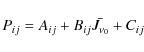
and follow a Planckian form (Fig. 2 - right hand
panel). The combined effect of the above processes, i.e. depopulation
and relatively unaffected source functions, leads to a smaller
,
and follow a Planckian form (Fig. 2 - right hand
panel). The combined effect of the above processes, i.e. depopulation
and relatively unaffected source functions, leads to a smaller ![]() and thus weaker lines, and increased abundances compared to the LTE
case. For stronger lines, forming further out in the atmosphere, there
is a divergence between
and thus weaker lines, and increased abundances compared to the LTE
case. For stronger lines, forming further out in the atmosphere, there
is a divergence between ![]() and
and ![]() and the source function thus diverges from the Planck function
(Fig. 2
- left hand panel). In the case where
and the source function thus diverges from the Planck function
(Fig. 2
- left hand panel). In the case where ![]() ,
the source function compensates slightly for the loss of opacity
leading to smaller NLTE corrections, the opposite being true for
,
the source function compensates slightly for the loss of opacity
leading to smaller NLTE corrections, the opposite being true for ![]() .
We see that for the lower level of the weaker line considered in the
figure has
.
We see that for the lower level of the weaker line considered in the
figure has ![]() ,
whilst
,
whilst ![]() ,
which leads to overionization of that level and greater departures than
the stronger line and greater NLTE abundance corrections.
,
which leads to overionization of that level and greater departures than
the stronger line and greater NLTE abundance corrections.
![\begin{figure}
\par\includegraphics[width=17.5cm,clip]{3693fg1.eps}
\end{figure}](/articles/aa/full_html/2010/03/aa13693-09/img67.png)
|
Figure 1:
Departure coefficients for all lower levels ( left)
and all upper levels ( right) of the lines we have
studied in the star HD 140283. A: |
| Open with DEXTER | |
|
Figure 2:
Source function, Sl,
mean intensity, |
| Open with DEXTER | |
The decrease in level population at ![]() 1 causes a drop in opacity for all lines. As a result of this, the
lines form deeper in the atmosphere than in LTE. In Fig. 3, we clearly
see this effect, where we show the continuum optical depth
1 causes a drop in opacity for all lines. As a result of this, the
lines form deeper in the atmosphere than in LTE. In Fig. 3, we clearly
see this effect, where we show the continuum optical depth ![]() at which the line optical depth
at which the line optical depth ![]() = 2/3. We also see that there is an increasingly large logarithmic
optical depth difference,
= 2/3. We also see that there is an increasingly large logarithmic
optical depth difference, ![]() ,
between the formation of weak lines in NLTE and LTE, up to
,
between the formation of weak lines in NLTE and LTE, up to ![]() 50 mÅ, after
which the difference becomes constant. With a decrease in opacity
compared to LTE, there needs to be an increase of abundance to match
the equivalent width of a given line in NLTE. Opacity is not the only
variable affected by NLTE, the source function can also be affected.
However, it is the dominant force in driving the NLTE departures within
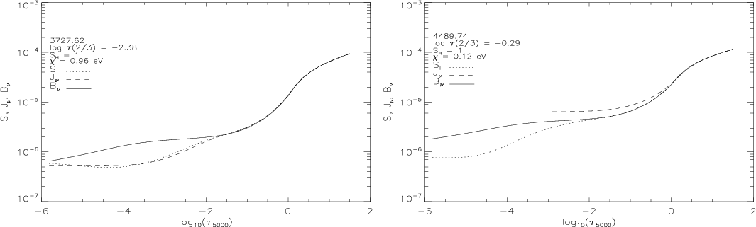
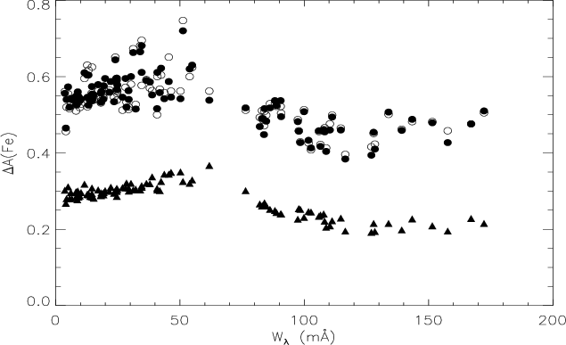
the Fe atom. In Fig. 4, we
plot the abundance correction versus equivalent width for the star
HD 140283. We see that there is a positive correction for the
different values of
50 mÅ, after
which the difference becomes constant. With a decrease in opacity
compared to LTE, there needs to be an increase of abundance to match
the equivalent width of a given line in NLTE. Opacity is not the only
variable affected by NLTE, the source function can also be affected.
However, it is the dominant force in driving the NLTE departures within
the Fe atom. In Fig. 4, we
plot the abundance correction versus equivalent width for the star
HD 140283. We see that there is a positive correction for the
different values of ![]() .
There is a clear trend with equivalent width. It is how this translates
to trends with excitation energy
.
There is a clear trend with equivalent width. It is how this translates
to trends with excitation energy ![]() that will affect
that will affect ![]() :
if the abundance corrections only shifted the mean abundance without
depending on
:
if the abundance corrections only shifted the mean abundance without
depending on ![]() then the derived
then the derived ![]() would not change.
would not change.
|
Figure 3:
The depth of formation of Fe I lines, with
no H collisions, on the log |
| Open with DEXTER | |
|
Figure 4:
Abundance correction versus equivalent width for the lines measured in
the star HD 140283 for |
| Open with DEXTER | |
Through Figs. 1 to 4 the general effects of NLTE on line formation can be seen. The depletion of level populations (Fig. 1) leads to a lower opacity and shifts the depth of formation to deeper levels (Fig. 3). This also means that a higher abundance is needed within NLTE, leading to positive abundance corrections (Fig. 4). However, there is a competing effect in some cases where the source function deviates from the Planck function (Fig. 2), which, in the case of the strong lines, compensates for the level depletion and decreases the abundance correction, as is seen in Fig. 4.
4 NLTE abundance corrections - deriving, testing, applying
In order to determine a new ![]() for a star, we first need to calculate NLTE corrections for the LTE
abundances derived in Paper I. Abundance corrections of the
form
for a star, we first need to calculate NLTE corrections for the LTE
abundances derived in Paper I. Abundance corrections of the
form ![]() -
- ![]() are calculated and applied to the LTE abundances from Paper I to
generate NLTE abundances on the same scale as that paper, rather than
using solely the new NLTE analysis. This procedure is used so as to tie
this work to the previous results, thus allowing the limitations of the
LTE assumptions in that work to be seen. To do this, a grid of MULTI
results for a range of abundances is created with increments of
0.02 dex. The abundance values covered by this grid depend on
the spread of abundances from individual lines in each star. MULTI
gives an LTE and NLTE equivalent width for each abundance in this grid.
A first step is to determine what
are calculated and applied to the LTE abundances from Paper I to
generate NLTE abundances on the same scale as that paper, rather than
using solely the new NLTE analysis. This procedure is used so as to tie
this work to the previous results, thus allowing the limitations of the
LTE assumptions in that work to be seen. To do this, a grid of MULTI
results for a range of abundances is created with increments of
0.02 dex. The abundance values covered by this grid depend on
the spread of abundances from individual lines in each star. MULTI
gives an LTE and NLTE equivalent width for each abundance in this grid.
A first step is to determine what ![]() from the MULTI grid corresponds to the LTE abundance derived in Paper I
(Hosford et al. 2009).
This is done for all Fe lines that are measured in the star. The NLTE
abundance inferred for a line is the abundance that corresponds to this
from the MULTI grid corresponds to the LTE abundance derived in Paper I
(Hosford et al. 2009).
This is done for all Fe lines that are measured in the star. The NLTE
abundance inferred for a line is the abundance that corresponds to this
![]() within the
grid of MULTI NLTE results. The correction is then calculated as
within the
grid of MULTI NLTE results. The correction is then calculated as ![]() =
= ![]() -
- ![]() .
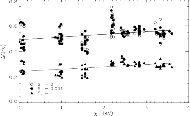
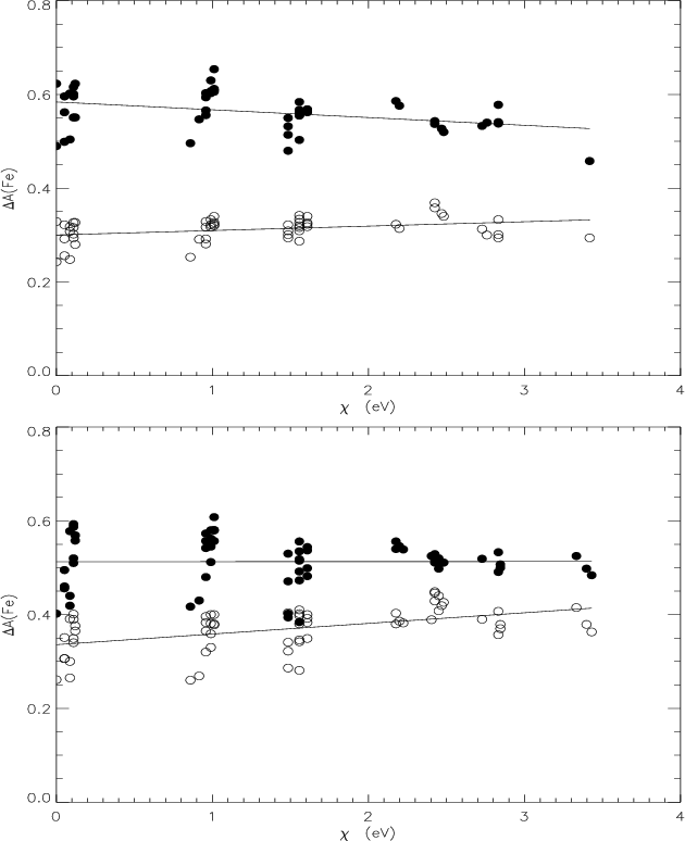
Figure 5
shows the corrections for the star HD 140283 calculated for
the three different
.
Figure 5
shows the corrections for the star HD 140283 calculated for
the three different ![]() values:
values: ![]() and 1. We see a trend in the abundance correction with
and 1. We see a trend in the abundance correction with ![]() ,
where we have values, from least square fits, of:
,
where we have values, from least square fits, of:
| (5) |
| (6) |
| (7) |
The non-zero coefficient of
|
Figure 5:
Abundance correction versus |
| Open with DEXTER | |
To test the corrections, we compared synthetic profiles from the NLTE
abundance with the observed profile, and compared measured ![]() 's with NLTE
's with NLTE
![]() 's from
MULTI, obtained from an abundance given by
's from
MULTI, obtained from an abundance given by ![]() +
+ ![]() .
The synthetic profiles are convolved with a Gaussian whose width is
allowed to vary from line to line. This represents the macroturbulent
and instrumental broadening, the latter calculated by fitting Gaussian
profiles to ThAr lines in IRAF and found to be
.
The synthetic profiles are convolved with a Gaussian whose width is
allowed to vary from line to line. This represents the macroturbulent
and instrumental broadening, the latter calculated by fitting Gaussian
profiles to ThAr lines in IRAF and found to be ![]() 100 mÅ. We found that the profiles match
the observed line reasonably well, and that measured and MULTI
calculated
100 mÅ. We found that the profiles match
the observed line reasonably well, and that measured and MULTI
calculated ![]() 's are
comparable, with a standard deviation of 2.3 mÅ. This gives us
confidence that the corrections are realistic within the framework of
the atomic model used. These corrections were then applied to the
WIDTH6 LTE abundances used in Paper I and new plots of
's are
comparable, with a standard deviation of 2.3 mÅ. This gives us
confidence that the corrections are realistic within the framework of
the atomic model used. These corrections were then applied to the
WIDTH6 LTE abundances used in Paper I and new plots of ![]() versus A(Fe) were plotted. We then nulled trends in
this plot to constrain
versus A(Fe) were plotted. We then nulled trends in
this plot to constrain ![]() (NLTE) by
recalculating the LTE abundances using the radiative transfer program
WIDTH6 (Kurucz & Furenlid 1978) exactly as in Hosford et al. (2009)
and reapplying the NLTE corrections, derived here from MULTI for the
original LTE parameters.
(NLTE) by
recalculating the LTE abundances using the radiative transfer program
WIDTH6 (Kurucz & Furenlid 1978) exactly as in Hosford et al. (2009)
and reapplying the NLTE corrections, derived here from MULTI for the
original LTE parameters.
Table 2:
Final ![]() and A(Li) for the selection of stars in this study.
and A(Li) for the selection of stars in this study.
As noted in Sect. 2.3, it
can be important to include the highest levels of the atom in the
calculations. It is not necessary to include each individual level
however, and it is possible to use superlevels that represent groups of
closely spaced levels (Korn 2008).
To test the effect of these upper levels, we took the approach of
giving the top 0.5 eV of levels in our atomic model an ![]() whilst the rest of the levels had
whilst the rest of the levels had ![]() .
We have done this for three situations; A) increasing
.
We have done this for three situations; A) increasing ![]() for just the bound-bound transitions rates, B) increasing
for just the bound-bound transitions rates, B) increasing ![]() for just the bound-free rates and C) increasing
for just the bound-free rates and C) increasing ![]() for both the bound-bound and bound-free. We discuss here only the case
of the bound-free rates as it is only these rates that have an effect,
edging the populations towards LTE values. Changing the bound-free
rates not only affects the higher levels but translates through all
lower ones. In fact it is the lower half of the atomic model that is
affected by a greater amount; further investigation into reasons for
this effect are discussed in Sect. 6.1. The
result can be seen in Fig. 6 where we
plot a level with
for both the bound-bound and bound-free. We discuss here only the case
of the bound-free rates as it is only these rates that have an effect,
edging the populations towards LTE values. Changing the bound-free
rates not only affects the higher levels but translates through all
lower ones. In fact it is the lower half of the atomic model that is
affected by a greater amount; further investigation into reasons for
this effect are discussed in Sect. 6.1. The
result can be seen in Fig. 6 where we
plot a level with ![]() eV
and one of the higher levels,
eV
and one of the higher levels, ![]() eV,
from our atomic model. Figure 7 shows
the abundance correction against
eV,
from our atomic model. Figure 7 shows
the abundance correction against ![]() for the increased
for the increased ![]() value of the upper levels and for a pure
value of the upper levels and for a pure ![]() situation. Comparing the differences in abundance correction between
situation. Comparing the differences in abundance correction between ![]() ,
and
,
and ![]() with
with ![]() on the upper levels we see a mean difference (
on the upper levels we see a mean difference (
![]() -
- ![]() )
of -0.031 dex for
)
of -0.031 dex for ![]() -2 eV and
-0.028 dex for
-2 eV and
-0.028 dex for ![]() eV,
for the star HD 140283. These effects equate to a 5 K
increase in
eV,
for the star HD 140283. These effects equate to a 5 K
increase in ![]() compared to
compared to ![]() .
It is then clear that the upper levels have a slight effect on the
final temperatures, and induce a slightly larger NLTE correction.
However, in the case of this study, where random errors are of order
.
It is then clear that the upper levels have a slight effect on the
final temperatures, and induce a slightly larger NLTE correction.
However, in the case of this study, where random errors are of order ![]() 80 K,
they will not make a significant effect.
80 K,
they will not make a significant effect.
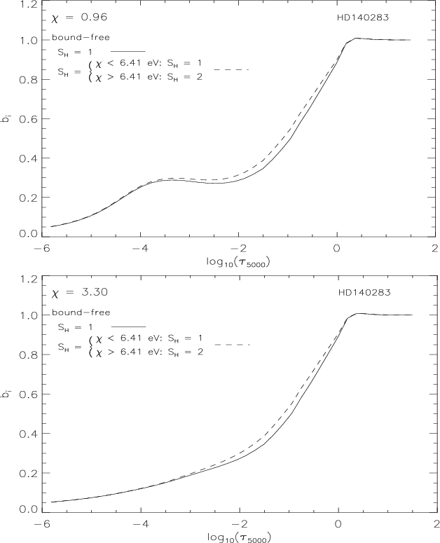
|
Figure 6:
Dashed line: the effects of increasing the |
| Open with DEXTER | |
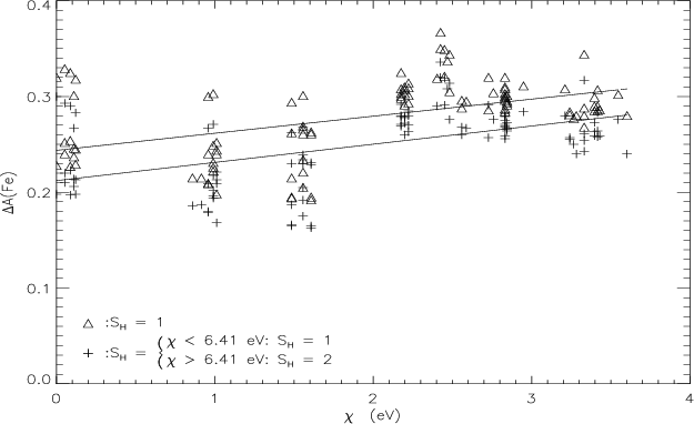
|
Figure 7:
Comparison between the abundance correction versus excitation energy
for the star HD 140283 using |
| Open with DEXTER | |
5 Results
Fe abundance corrections for the stars in Table 1 have been
calculated and new temperatures have been derived using the excitation
energy technique, as in Paper I but with the NLTE corrections applied
as described in Sect. 4.
Table 2
lists the new NLTE ![]() 's and
's and ![]() ,
such that
,
such that ![]() =
= ![]() -
- ![]() ,
for the selection of stars.
,
for the selection of stars.
For this work, all the other parameters, viz. log g,
[Fe/H] and ![]() ,
were kept at the values found in Hosford
et al. (2009). Our aim here, as it was in Hosford et al. (2009),
is to narrow down the zero point of the temperature scale by
quantifying the systematic errors, albeit at the expense of having
larger star to star random errors. Contributions to the errors come
from adopted gravity, the nulling procedure in determining the
,
were kept at the values found in Hosford
et al. (2009). Our aim here, as it was in Hosford et al. (2009),
is to narrow down the zero point of the temperature scale by
quantifying the systematic errors, albeit at the expense of having
larger star to star random errors. Contributions to the errors come
from adopted gravity, the nulling procedure in determining the ![]() ,
and smaller contributions from the error in microturbulence, errors in
the age, metallicity and initial temperature,
,
and smaller contributions from the error in microturbulence, errors in
the age, metallicity and initial temperature, ![]() ,
when determining isochronal gravities. In relation to the gravities,
the three HD stars had gravities derived using HIPPARCOS
parallaxes, and their errors are a reflection of errors propagating
through this calculation, whilst for the remaining stars isochrones
were used. The isochronal gravities are sensitive to age, with a 1 Gyr
difference leading to a change of
,
when determining isochronal gravities. In relation to the gravities,
the three HD stars had gravities derived using HIPPARCOS
parallaxes, and their errors are a reflection of errors propagating
through this calculation, whilst for the remaining stars isochrones
were used. The isochronal gravities are sensitive to age, with a 1 Gyr
difference leading to a change of ![]() 0.03 dex for main sequence (MS) stars
and
0.03 dex for main sequence (MS) stars
and ![]() 0.06 dex
for sub-giant (SGB) stars. This equates to a change in
0.06 dex
for sub-giant (SGB) stars. This equates to a change in ![]() of 12 K and 24 K respectively. These errors are based
on LTE sensitivities, as are other errors quoted below. There is also a
dependence on the initial temperature, a photometric temperature from
Ryan et al. (1999), used to determine the isochronal gravity.
A +100 K difference leads to +0.06 dex and -0.06 dex
for MS and SGB stars respectively. This equates to
of 12 K and 24 K respectively. These errors are based
on LTE sensitivities, as are other errors quoted below. There is also a
dependence on the initial temperature, a photometric temperature from
Ryan et al. (1999), used to determine the isochronal gravity.
A +100 K difference leads to +0.06 dex and -0.06 dex
for MS and SGB stars respectively. This equates to ![]() 24 K
in
24 K
in ![]() which shows, importantly, that
which shows, importantly, that ![]() is only weakly dependent on the initial photometric temperature.
Contributions to
is only weakly dependent on the initial photometric temperature.
Contributions to ![]() is also sensitive to microturbulence, for which an error of
is also sensitive to microturbulence, for which an error of ![]() 0.1 km
0.1 km
![]() equates to an error of
equates to an error of ![]() 60 K.
60 K.
In the nulling procedure any trends between [Fe/H] and ![]() are removed. Due to the range in line to line Fe abundances for a
particular star, there is a statistical error in the trend which is of
order
are removed. Due to the range in line to line Fe abundances for a
particular star, there is a statistical error in the trend which is of
order ![]() dex
per eV, which equates to
dex
per eV, which equates to ![]() 40-100 K depending on
the star under study. This error also contains the random line-to-line
errors due to equivalent width, gf, and damping
values. The final
40-100 K depending on
the star under study. This error also contains the random line-to-line
errors due to equivalent width, gf, and damping
values. The final ![]() error in Table 2
is then a conflation of this statistical error and the errors from
error in Table 2
is then a conflation of this statistical error and the errors from ![]() age =
1 Gyr,
age =
1 Gyr, ![]() km
km
![]() ,
,
![]() [Fe/H] =
0.05 and
[Fe/H] =
0.05 and ![]() K.
K.
These new ![]() values and equivalent widths from Ryan
et al. (1999) were then used to calculate new Li by
interpolating within a grid of equivalent width versus abundance for
different
values and equivalent widths from Ryan
et al. (1999) were then used to calculate new Li by
interpolating within a grid of equivalent width versus abundance for
different ![]() .
This grid was taken from Ryan
et al. (1996a).
.
This grid was taken from Ryan
et al. (1996a).
6 Discussion
6.1 The  scale
scale
With the addition of the NLTE corrections, we see in Table 2 that there is, for
the most part, an increase in ![]() from the LTE
from the LTE ![]() 's of Hosford et al. (2009),
for both cases of
's of Hosford et al. (2009),
for both cases of ![]() .
The only exception is CD-33
.
The only exception is CD-33![]() 1173 in the
1173 in the ![]() case, for which there is a 93 K decrease. We return to this star below.
The
case, for which there is a 93 K decrease. We return to this star below.
The ![]() corrections we have derived average 59 K for
corrections we have derived average 59 K for ![]() and 73 K for
and 73 K for ![]() (treating LP 815-43 as one datum, not two). For
(treating LP 815-43 as one datum, not two). For ![]() the temperature corrections tend to increase at cooler temperatures,
whilst the tendency is weaker or opposite for
the temperature corrections tend to increase at cooler temperatures,
whilst the tendency is weaker or opposite for ![]() ,
i.e. corrections increase at higher temperatures (obviously the gravity
and metallicity of the stars also affects their NLTE corrections, but
nevertheless we find it intsructive to consider temperature as one
useful discriminating variable). This gives rise to a change in the
difference
,
i.e. corrections increase at higher temperatures (obviously the gravity
and metallicity of the stars also affects their NLTE corrections, but
nevertheless we find it intsructive to consider temperature as one
useful discriminating variable). This gives rise to a change in the
difference ![]() with temperature, with this quantity being negative for the two hottest
stars, CD-33
with temperature, with this quantity being negative for the two hottest
stars, CD-33![]() 1173
and LP 815-43. The switch over from
1173
and LP 815-43. The switch over from ![]() having the larger correction to
having the larger correction to ![]() having the larger correction is at around
having the larger correction is at around ![]() 6200 K. Further testing has shown that this is not a random
error and is clearly something to investigate further in the future.
This is further shown by Fig. 8 where
the abundance correction versus
6200 K. Further testing has shown that this is not a random
error and is clearly something to investigate further in the future.
This is further shown by Fig. 8 where
the abundance correction versus ![]() for the stars CD-33
for the stars CD-33![]() 1173
and LP 815-43 (SGB) are plotted. It is seen that for
LP 815-43 (SGB), increasing
1173
and LP 815-43 (SGB) are plotted. It is seen that for
LP 815-43 (SGB), increasing ![]() has a larger effect on the lower excitation lines than for higher ones.
This has induced a trend of abundance with
has a larger effect on the lower excitation lines than for higher ones.
This has induced a trend of abundance with ![]() larger than that of the
larger than that of the ![]() case. This in turn leads to a larger temperature correction for
case. This in turn leads to a larger temperature correction for ![]() than for
than for ![]() .
The reason for this effect is still uncertain.
.
The reason for this effect is still uncertain.
To investigate this behaviour further, the test of increasing
the ![]() value of the upper levels, as done on HD 140283 in
Sect. 4, has also been performed on LP 815-43 for the
MS and SGB parameters. This has shown that the effect of collisions
with neutral H are indeed larger for the lower levels of the atom, and
that this effect is larger for LP 815-43 (MS), which is the
hottest star. This indicates that there is a temperature dependence,
i.e. the difference between the mean difference (
value of the upper levels, as done on HD 140283 in
Sect. 4, has also been performed on LP 815-43 for the
MS and SGB parameters. This has shown that the effect of collisions
with neutral H are indeed larger for the lower levels of the atom, and
that this effect is larger for LP 815-43 (MS), which is the
hottest star. This indicates that there is a temperature dependence,
i.e. the difference between the mean difference (
![]() -
- ![]() )
(where
)
(where ![]() indicates the scenario of having
indicates the scenario of having ![]() for the top 0.5 eV worth of levels) for the levels with
for the top 0.5 eV worth of levels) for the levels with ![]() eV
and those with
eV
and those with ![]() eV
is greater for the hotter star, LP 815-43 (MS). However, when
performing this test on LP 815-43 (SGB), which has a similar
log g to HD 140283 whilst still being
hotter, the effect is not as great as for HD 140283. This
shows that there is some gravity dependence on the neutral H collisions
along with the temperature dependence i.e. the gravity indirectly
affects the collisional rates, by impacting on the number density of
hydrogen atoms at a given optical depth. Figure 8, along
with Fig. 5,
clearly show that NLTE has varying star to star effects, i.e. from the
similar effects at different
eV
is greater for the hotter star, LP 815-43 (MS). However, when
performing this test on LP 815-43 (SGB), which has a similar
log g to HD 140283 whilst still being
hotter, the effect is not as great as for HD 140283. This
shows that there is some gravity dependence on the neutral H collisions
along with the temperature dependence i.e. the gravity indirectly
affects the collisional rates, by impacting on the number density of
hydrogen atoms at a given optical depth. Figure 8, along
with Fig. 5,
clearly show that NLTE has varying star to star effects, i.e. from the
similar effects at different ![]() values in HD 140283 (Fig. 5),
to the differing effects in CD-33
values in HD 140283 (Fig. 5),
to the differing effects in CD-33![]() 1173 and LP 815-43
(SGB) (Fig. 8).
The range of
1173 and LP 815-43
(SGB) (Fig. 8).
The range of ![]() values, and the negative value for CD-33
values, and the negative value for CD-33![]() 1173, shows the intricacies of
the NLTE process, and that generalisations are not easily made when
identifying the effects of NLTE on temperatures determined by the
excitation energy method. For the purposes of this paper, which is
concerned with the effective temperatures in the context of the
available NLTE model, it is appropriate to acknowledge these NLTE
effects and to move ahead to use them in the study of the Li problem,
whilst still recognising that much work remains before we approach a
complete description of the Fe atom.
1173, shows the intricacies of
the NLTE process, and that generalisations are not easily made when
identifying the effects of NLTE on temperatures determined by the
excitation energy method. For the purposes of this paper, which is
concerned with the effective temperatures in the context of the
available NLTE model, it is appropriate to acknowledge these NLTE
effects and to move ahead to use them in the study of the Li problem,
whilst still recognising that much work remains before we approach a
complete description of the Fe atom.
|
Figure 8:
Abudance correction versus |
| Open with DEXTER | |
Although we discussed the possibility that the extreme (negative) ![]() correction for CD-33
correction for CD-33![]() 1173
is due to corrrections being temperature-dependent, this unusual case
may be in part due to the fact that only a subset of the original lines
measured is available through the NLTE atomic model. The atomic model
does not contain every level of the Fe atom and therefore some
transitions are not present in the calculations. This means that not
every line measured for a given star is present in the calculations and
leads to a trend being introduced in the
1173
is due to corrrections being temperature-dependent, this unusual case
may be in part due to the fact that only a subset of the original lines
measured is available through the NLTE atomic model. The atomic model
does not contain every level of the Fe atom and therefore some
transitions are not present in the calculations. This means that not
every line measured for a given star is present in the calculations and
leads to a trend being introduced in the ![]() -abundance plot prior to the
trend induced by the NLTE corrections. This is because the original
nulling of the
-abundance plot prior to the
trend induced by the NLTE corrections. This is because the original
nulling of the ![]() -abundance
plot was achieved with a greater number of points. CD-33
-abundance
plot was achieved with a greater number of points. CD-33![]() 1173 has the
least lines available from the atomic model used with MULTI, however,
there is no distinct trend between
1173 has the
least lines available from the atomic model used with MULTI, however,
there is no distinct trend between ![]() and the number of lines available for each star, and after testing we
found that the effect of the subset, i.e. the measured lines that are
available with our atomic model, is to increase the LTE temperature.
This implies that the decrease in
and the number of lines available for each star, and after testing we
found that the effect of the subset, i.e. the measured lines that are
available with our atomic model, is to increase the LTE temperature.
This implies that the decrease in ![]() for this star is most likely due to NLTE effects. Although there is no
obvious correlation between the number of lines available and the
temperature correction, this emphasises the need for a complete atomic
model. This is especially true when considering the abundance of
individual lines, as in the excitation technique used in this work.
for this star is most likely due to NLTE effects. Although there is no
obvious correlation between the number of lines available and the
temperature correction, this emphasises the need for a complete atomic
model. This is especially true when considering the abundance of
individual lines, as in the excitation technique used in this work.
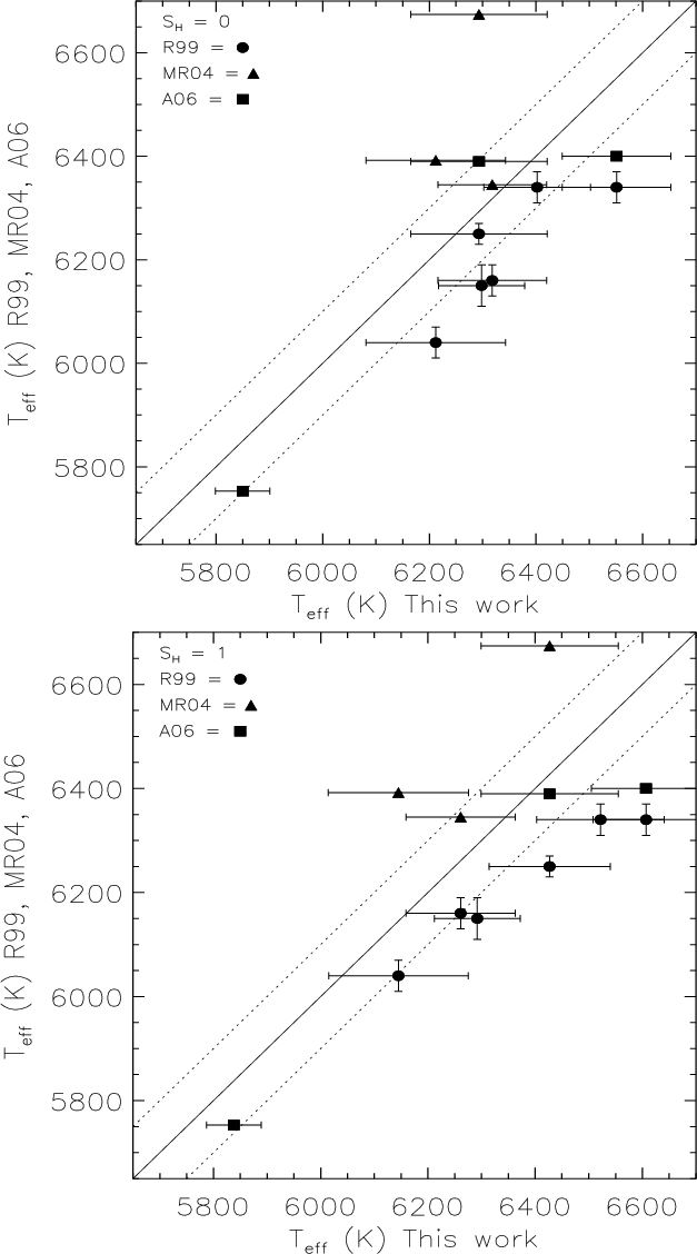
As in Paper I, we have compared our ![]() values with those of Ryan
et al. (1999), Meléndez
& Ramírez (2004), and Asplund
et al. (2006). Figure 9 presents
these comparisons. Comparing against the photometric temperatures of Ryan et al. (1999)
for five stars in common, we see that our new
values with those of Ryan
et al. (1999), Meléndez
& Ramírez (2004), and Asplund
et al. (2006). Figure 9 presents
these comparisons. Comparing against the photometric temperatures of Ryan et al. (1999)
for five stars in common, we see that our new ![]() scale is hotter by an average of 132 K, with a minimum and maximum of
43 K and 211 K respectively for an
scale is hotter by an average of 132 K, with a minimum and maximum of
43 K and 211 K respectively for an ![]() .
Recall that
.
Recall that ![]() corresponds to the maximal NLTE effect, i.e. no collisions with the
hydrogen, for the model atom we have adopted. For
corresponds to the maximal NLTE effect, i.e. no collisions with the
hydrogen, for the model atom we have adopted. For ![]() ,
our scale is hotter by an average of 162 K, with a minimum and maximum
of 101 K and 267 K respectively.
,
our scale is hotter by an average of 162 K, with a minimum and maximum
of 101 K and 267 K respectively.
|
Figure 9:
|
| Open with DEXTER | |
We have three stars in common with Meléndez
& Ramírez (2004). Their temperatures are hotter than
the ones we derived here by 196 K on average for ![]() with a minimum and maximum difference of 27 K and
381 K respectively, and by 193 K on average for
with a minimum and maximum difference of 27 K and
381 K respectively, and by 193 K on average for ![]() ,
with a minimum and maximum difference of 84 K and
247 K respectively. Therefore, even with NLTE corrections we
still cannot achieve the high
,
with a minimum and maximum difference of 84 K and
247 K respectively. Therefore, even with NLTE corrections we
still cannot achieve the high ![]() of the Meléndez &
Ramírez (2004) study. It has however been noted (Mel
of the Meléndez &
Ramírez (2004) study. It has however been noted (Mel
![]() ndez 2009 - private
communication) that the Meléndez
& Ramírez (2004) temperatures suffer from systematic
errors due a imperfect calibration of the bolometric correction for the
choice of photometric bands used. This led to an inaccurate zero point
and hotter
ndez 2009 - private
communication) that the Meléndez
& Ramírez (2004) temperatures suffer from systematic
errors due a imperfect calibration of the bolometric correction for the
choice of photometric bands used. This led to an inaccurate zero point
and hotter ![]() 's than most
other studies. The revision of their temperature scale is not yet
available and comparisons to their new
's than most
other studies. The revision of their temperature scale is not yet
available and comparisons to their new ![]() 's is not
possible at this time.
's is not
possible at this time.
Finally, we have three stars in common with Asplund et al. (2006).
Using ![]() we obtain temperatures for two of the stars that are hotter than Asplund et al. (2006)
by 97 K and 151 K. The third star is CD-33
we obtain temperatures for two of the stars that are hotter than Asplund et al. (2006)
by 97 K and 151 K. The third star is CD-33![]() 1173, for
which we calculated a negative temperature correction, and which is
cooler in our study by 97 K. The temperatures for all three
stars are hotter in our study than in Asplund
et al. (2006) when using
1173, for
which we calculated a negative temperature correction, and which is
cooler in our study by 97 K. The temperatures for all three
stars are hotter in our study than in Asplund
et al. (2006) when using ![]() .
Here the average difference is 110 K, values ranging from
37 K to 207 K. If the Asplund
et al. (2006) temperatures are affected by NLTE, as
stated by Barklem (2007)
who expects a 100 K increase in Balmer line temperatures, this would
bring the
.
Here the average difference is 110 K, values ranging from
37 K to 207 K. If the Asplund
et al. (2006) temperatures are affected by NLTE, as
stated by Barklem (2007)
who expects a 100 K increase in Balmer line temperatures, this would
bring the ![]() scales back into agreement. Another problem facing the Balmer line
method is the effects of granulation, due to convection, on the line
wings (Ludwig et al.
2009). It has been found (Bonifacio - private communication)
that inclusion of these effects would increase the effective
temperatures derived with this method. In particular a value of
scales back into agreement. Another problem facing the Balmer line
method is the effects of granulation, due to convection, on the line
wings (Ludwig et al.
2009). It has been found (Bonifacio - private communication)
that inclusion of these effects would increase the effective
temperatures derived with this method. In particular a value of ![]() = 6578 K has been found for the star LP 815-43. Although this
is 176 K hotter than our result for the SGB case with
= 6578 K has been found for the star LP 815-43. Although this
is 176 K hotter than our result for the SGB case with ![]() ,
i.e.
,
i.e. ![]() K,
it is in good agreement with the values
K,
it is in good agreement with the values ![]() = 6522 K (
= 6522 K (
![]() )
for the SGB case and
)
for the SGB case and ![]() K
(
K
(
![]() )
or
)
or ![]() K
(
K
(
![]() )
for the MS case, calculated in this work.
)
for the MS case, calculated in this work.
6.2 Lithium abundances
We now address the new Li abundances and their effect on the lithium
problem. We see that the introduction of NLTE corrections to the ![]() scale has led to temperatures that are of order 100 K hotter than LTE
temperature scales, with the obvious exception of the Meléndez & Ramírez (2004)
scale. This will then lead to an increase in the mean lithium
abundance. Table 2
lists A(Li) for the new temperatures. With these
new
scale has led to temperatures that are of order 100 K hotter than LTE
temperature scales, with the obvious exception of the Meléndez & Ramírez (2004)
scale. This will then lead to an increase in the mean lithium
abundance. Table 2
lists A(Li) for the new temperatures. With these
new ![]() 's, we calculate a mean Li
abundance of A(Li) = 2.19 dex with a
scatter of 0.072 dex when using
's, we calculate a mean Li
abundance of A(Li) = 2.19 dex with a
scatter of 0.072 dex when using ![]() ,
and A(Li) = 2.21 dex with a scatter of
0.058 dex for the
,
and A(Li) = 2.21 dex with a scatter of
0.058 dex for the ![]() case. Consistent with the temperature increase, these values are higher
than those found by other studies, in particular Spite et al. (1996),
who found a value of A(Li) = 2.08 (
case. Consistent with the temperature increase, these values are higher
than those found by other studies, in particular Spite et al. (1996),
who found a value of A(Li) = 2.08 (![]() 0.08) dex
using a similar iron excitation energy technique but without the NLTE
corrections, Bonifacio
et al. (2007) with A(Li) = 2.10 (
0.08) dex
using a similar iron excitation energy technique but without the NLTE
corrections, Bonifacio
et al. (2007) with A(Li) = 2.10 (![]() 0.09) using
a Balmer line wing temperature scale, and A(Li) =
2.16 dex or A(Li) = 2.10 depending on the
evolutionary state from Hosford
et al. (2009). The NLTE corrections have moved the
mean Li abundance closer to, but not consistent with, the WMAP value of
A(Li) = 2.72 dex, and thus still leaves the
lithium problem unsolved. It is noted that even the Meléndez & Ramírez (2004)
scale, whilst bringing the observed and theoretical Li abundances
closer, still failed to solve the lithium problem.
0.09) using
a Balmer line wing temperature scale, and A(Li) =
2.16 dex or A(Li) = 2.10 depending on the
evolutionary state from Hosford
et al. (2009). The NLTE corrections have moved the
mean Li abundance closer to, but not consistent with, the WMAP value of
A(Li) = 2.72 dex, and thus still leaves the
lithium problem unsolved. It is noted that even the Meléndez & Ramírez (2004)
scale, whilst bringing the observed and theoretical Li abundances
closer, still failed to solve the lithium problem.
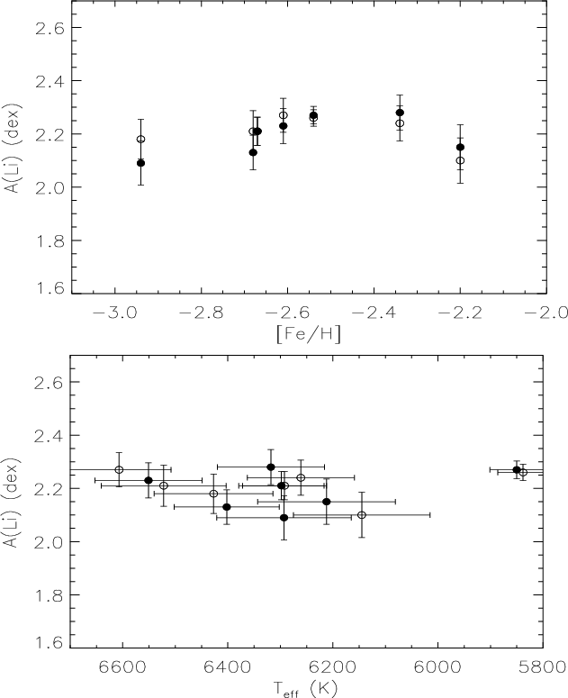
|
Figure 10:
Lithium abundance versus [Fe/H] ( top panel) and |
| Open with DEXTER | |
Figure 10
shows the lithium abundances versus [Fe/H] and ![]() ,
least squares fits have been performed for both sets of data. In the
fit to metallicity we get the values:
,
least squares fits have been performed for both sets of data. In the
fit to metallicity we get the values:
for
for
| (10) |
for
| (11) |
for
We also perform the fit as described by Ryan et al. (2000), such that:
|
(12) |
where
We see then that the addition of NLTE corrections has led to
an increase in ![]() for most stars. This equates to an increase in A(Li)
but it is still not high enough to reconcile the lithium problem.
Through the efforts of Hosford
et al. (2009) and this study it is safe to conclude
that systematic errors in the metal-poor
for most stars. This equates to an increase in A(Li)
but it is still not high enough to reconcile the lithium problem.
Through the efforts of Hosford
et al. (2009) and this study it is safe to conclude
that systematic errors in the metal-poor ![]() scale are almost certainly not large enough to be the source of the A(Li)
discrepancy between observation and WMAP + BBN predictions. This
outcome lends strength to other possible explanations, such as
processing in the stars, e.g. diffusion, processing in earlier
generations of stars, and/or different BBN networks, or more exotic
solutions requiring physics beyond the standard model.
scale are almost certainly not large enough to be the source of the A(Li)
discrepancy between observation and WMAP + BBN predictions. This
outcome lends strength to other possible explanations, such as
processing in the stars, e.g. diffusion, processing in earlier
generations of stars, and/or different BBN networks, or more exotic
solutions requiring physics beyond the standard model.
It should be noted that while we have computed Fe lines in
NLTE to constrain the temperature, our Li abundances are calculated
from a grid of abundance versus equivalent width that was constructed
under the assumptions of LTE, see Paper I for details. Several studies
of the effects of NLTE Li line formation have been conducted. Two of
these studies are those of Carlsson
et al. (1994) and Lind
et al. (2009); they find Li abundance corrections of
![]() +0.013-+0.020 dex
and
+0.013-+0.020 dex
and ![]() +0.01-+0.03 dex
respectively for the temperature, log g and [Fe/H] range in this study.
Due to the very small size of these corrections we find the use of the
LTE grid, combined with our NLTE effective temperatures, to be
acceptable in determining Li abundances, and that the introduction of
NLTE Li abundances will not significantly aid in solving the lithium
problem.
+0.01-+0.03 dex
respectively for the temperature, log g and [Fe/H] range in this study.
Due to the very small size of these corrections we find the use of the
LTE grid, combined with our NLTE effective temperatures, to be
acceptable in determining Li abundances, and that the introduction of
NLTE Li abundances will not significantly aid in solving the lithium
problem.
6.3 Implications of NLTE calculations for ionization balance and S
Having discussed the effects of NLTE corrections on the ![]() scale and the lithium abundances, it is also of interest to note the
effect on an aspect of abundance analysis, specifically ionization
equilibrium often used in the determination of log g.
We can also make a preliminary investigation into constraints we can
place on the value of
scale and the lithium abundances, it is also of interest to note the
effect on an aspect of abundance analysis, specifically ionization
equilibrium often used in the determination of log g.
We can also make a preliminary investigation into constraints we can
place on the value of ![]() from our results.
from our results.
It has been noted previously (Gehren
et al. 2001) that Fe II
lines are relatively unaffected by NLTE. In this work we have also
found this to be the case with values for Fe II
abundance corrections of order 0.01 dex. Our NLTE calculations
induce a mean difference between ![]() (Fe I)
and
(Fe I)
and ![]() (Fe
II) of 0.39 dex for
(Fe
II) of 0.39 dex for ![]() and 0.27 dex for
and 0.27 dex for ![]() .
Knowing that a 0.1 dex change in log g induces a difference of
0.05 dex between Fe I and Fe II
abundance, for there to be ionization balance, one would need a
correction of
.
Knowing that a 0.1 dex change in log g induces a difference of
0.05 dex between Fe I and Fe II
abundance, for there to be ionization balance, one would need a
correction of ![]() +0.8 dex
and +0.5 dex in log g for
+0.8 dex
and +0.5 dex in log g for ![]() and 1 respectively. That is, due to overionization, forcing ionization
balance for metal-poor dwarfs under LTE calculations would give
log g values too low by 0.8 dex (
and 1 respectively. That is, due to overionization, forcing ionization
balance for metal-poor dwarfs under LTE calculations would give
log g values too low by 0.8 dex (
![]() )
or 0.5 dex (
)
or 0.5 dex (
![]() ). LTE calculations for
HD 140283 have occasionally yielded gravities lower than the HIPPARCOS
gravity by
). LTE calculations for
HD 140283 have occasionally yielded gravities lower than the HIPPARCOS
gravity by ![]() 0.3
(e.g. Ryan et al. 1996b),
and for a selection of 13 halo main sequance turnoff stars with HIPPARCOS
parallaxes Ryan et al. (2009 - in preperation) determine a
mean difference of 0.2 in log g compared to LTE
ionization balance. These differences are less than what we compute for
0.3
(e.g. Ryan et al. 1996b),
and for a selection of 13 halo main sequance turnoff stars with HIPPARCOS
parallaxes Ryan et al. (2009 - in preperation) determine a
mean difference of 0.2 in log g compared to LTE
ionization balance. These differences are less than what we compute for
![]() ,
and suggest that for the model atom we are using, the choice of
,
and suggest that for the model atom we are using, the choice of ![]() may underestimate the role of collisions with neutral hydrogen in
diminishing the departures from LTE for Fe, i.e. that
may underestimate the role of collisions with neutral hydrogen in
diminishing the departures from LTE for Fe, i.e. that ![]() .
Whilst we have not attempted a detailed derivation of
.
Whilst we have not attempted a detailed derivation of ![]() by this method, Korn
et al. (2003) has, arriving at a value of
by this method, Korn
et al. (2003) has, arriving at a value of ![]() based on the analysis of four halo stars and two others. Our results
are broadly consistent with their conclusion.
based on the analysis of four halo stars and two others. Our results
are broadly consistent with their conclusion.
7 Conclusions
We have discussed the processes of NLTE line formation of Fe lines.
Here, we have shown the challenges posed by such calculations and the
uncertainties that still arise, in particular due to the unknown
magnitude of H collisions. As there is at present no better theoretical
or experimental description of the role of H collisions, one obvious
next step would be to tie down the value of ![]() for metal-poor stars, for example by forcing the equality of HIPPARCOS
gravities and those determined by ionization equilibrium by changing
for metal-poor stars, for example by forcing the equality of HIPPARCOS
gravities and those determined by ionization equilibrium by changing ![]() (Korn et al. 2003).
For this reason we have discussed the effect of NLTE corrections on the
ionization equilibrium and the magnitude of the effect on log g.
(Korn et al. 2003).
For this reason we have discussed the effect of NLTE corrections on the
ionization equilibrium and the magnitude of the effect on log g.
Six of the original program stars from Paper I have been
analysed to calculate the effects of NLTE on the ![]() scale derived from Fe I lines via
excitation equilibrium. We have found that the effect of the correction
is to cause an increase in
scale derived from Fe I lines via
excitation equilibrium. We have found that the effect of the correction
is to cause an increase in ![]() ranging from 2 K to 150 K for
ranging from 2 K to 150 K for ![]() and 41 K to 122 K for
and 41 K to 122 K for ![]() .
There is one exception; the star CD-33
.
There is one exception; the star CD-33![]() 1173 has a negative correction
(-93 K) for the
1173 has a negative correction
(-93 K) for the ![]() case. This may be due to the limited number of Fe lines available for
this star, but also emphasises the intricacies of NLTE work which make
it difficult to make reliable generalisations.
case. This may be due to the limited number of Fe lines available for
this star, but also emphasises the intricacies of NLTE work which make
it difficult to make reliable generalisations.
Our new temperatures have been compared to the photometric
temperatures of Ryan
et al. (1999), the IRFM of Meléndez & Ramírez (2004),
and the Balmer line wing method of Asplund
et al. (2006). We find that the NLTE temperatures
are hotter than Ryan
et al. (1999) by an average of 132 K for ![]() and 162 K for
and 162 K for ![]() .
Similar results are found when comparing against Asplund et al. (2006)
with average differences of 76 K and 110 K for
.
Similar results are found when comparing against Asplund et al. (2006)
with average differences of 76 K and 110 K for ![]() and 1 respectively. The difference between our temperatures and the Asplund et al. (2006)
temperatures may be removed if the Balmer line wing method suffers from
NLTE effects (Barklem 2007),
or the effects of granulation are properly described. We find that even
with NLTE corrections we are unable to match the high
and 1 respectively. The difference between our temperatures and the Asplund et al. (2006)
temperatures may be removed if the Balmer line wing method suffers from
NLTE effects (Barklem 2007),
or the effects of granulation are properly described. We find that even
with NLTE corrections we are unable to match the high ![]() 's of Meléndez & Ramírez (2004).
However, it has been acknowledged that their temperatures suffer from
systematic errors (Mel
's of Meléndez & Ramírez (2004).
However, it has been acknowledged that their temperatures suffer from
systematic errors (Mel
![]() ndez 2009 - private
communication) and a revision of their temperature scale is under way.
ndez 2009 - private
communication) and a revision of their temperature scale is under way.
With our new ![]() scale, new Li abundances have been calculated. This has led to an
increase of the mean Li abundance from Hosford
et al. (2009) to values of 2.19 dex with a
scatter of 0.07 dex and 2.21 dex with a scatter of
0.06 dex for
scale, new Li abundances have been calculated. This has led to an
increase of the mean Li abundance from Hosford
et al. (2009) to values of 2.19 dex with a
scatter of 0.07 dex and 2.21 dex with a scatter of
0.06 dex for ![]() and 1 respectively, both of which lie well below the value of
2.72 dex inferred from WMAP+BBN (Cyburt
et al. 2008). This has shown that systematic errors
in the
and 1 respectively, both of which lie well below the value of
2.72 dex inferred from WMAP+BBN (Cyburt
et al. 2008). This has shown that systematic errors
in the ![]() scale of metal-poor stars are not the cause for the discrepency.
scale of metal-poor stars are not the cause for the discrepency.
The authors thank A. J. Korn for his discussions on the processes of NLTE and suggestions on how to proceed with this study. S.G.R. and A.E.G.P. gratefully acknowledge the support from the Royal Society under International Joint Project 2006/23 involving colleagues at Uppsala University. A.H. and A.E.G.P. thank the STFC for its financial support to do this work. The work of K.O. was supported in part by DOE grant DE-FG02-94ER-40823 at the University of Minnesota.
References
- Alonso, A., Arribas, S., & Martinez-Roger, C. 1996, A&AS, 117, 227 [NASA ADS] [CrossRef] [EDP Sciences] [Google Scholar]
- Aoki, W., Barklem, P. S., Beers, T. C., et al. 2009, ApJ, 698, 1803 [NASA ADS] [CrossRef] [Google Scholar]
- Asplund, M. 2005, ARA&A, 43, 481 [NASA ADS] [CrossRef] [Google Scholar]
- Asplund, M., Gustafsson, B., Kiselman, D., & Eriksson, K. 1997, A&A, 318, 521 [NASA ADS] [Google Scholar]
- Asplund, M., Nordlund, Å., Trampedach, R., & Stein, R. F. 1999, A&A, 346, L17 [NASA ADS] [Google Scholar]
- Asplund, M., Lambert, D. L., Nissen, P. E., Primas, F., & Smith, V. V. 2006, ApJ, 644, 229 [NASA ADS] [CrossRef] [Google Scholar]
- Barklem, P. S. 2007, A&A, 466, 327 [NASA ADS] [CrossRef] [EDP Sciences] [Google Scholar]
- Barklem, P. S., Belyaev, A. K., & Asplund, M. 2003, A&A, 409, L1 [NASA ADS] [CrossRef] [EDP Sciences] [Google Scholar]
- Bautista, M. A. 1997, A&AS, 122, 167 [Google Scholar]
- Bonifacio, P., Molaro, P., Sivarani, T., et al. 2007, A&A, 462, 851 [NASA ADS] [CrossRef] [EDP Sciences] [Google Scholar]
- Carlsson, M. 1986, Uppsala Astronomical Observatory Reports, 33 [Google Scholar]
- Carlsson, M., Rutten, R. J., Bruls, J. H. M. J., & Shchukina, N. G. 1994, A&A, 288, 860 [NASA ADS] [Google Scholar]
- Collet, R., Asplund, M., & Thévenin, F. 2005, A&A, 442, 643 [NASA ADS] [CrossRef] [EDP Sciences] [MathSciNet] [Google Scholar]
- Cox, A. N. 2000, S&T, 100, 010000 [Google Scholar]
- Cyburt, R. H., Fields, B. D., & Olive, K. A. 2008, J. Cosmol. Astro-Part. Phys., 11, 12 [Google Scholar]
- Drawin, H. W. 1968, Z. Phys., 211, 404 [Google Scholar]
- Drawin, H. W. 1969, Z. Phys., 225, 483 [Google Scholar]
- Fleck, I., Grosser, J., Schnecke, A., Steen, W., & Voigt, H. 1991, J. Phys. B, 24, 4017 [Google Scholar]
- Fuhr, J. R., Martin, G. A., & Wiese, W. L. 1988, Atomic transition probabilities, Iron through Nickel, ed. J. R. Fuhr, G. A. Martin, & W. L. Wiese [Google Scholar]
- Fuhrmann, K., Axer, M., & Gehren, T. 1994, A&A, 285, 585 [NASA ADS] [Google Scholar]
- Gehren, T., Butler, K., Mashonkina, L., Reetz, J., & Shi, J. 2001, A&A, 366, 981 [NASA ADS] [CrossRef] [EDP Sciences] [Google Scholar]
- Gratton, R. G., Carretta, E., Eriksson, K., & Gustafsson, B. 1999, A&A, 350, 955 [NASA ADS] [Google Scholar]
- Hirata, R., & Horaguchi, T. 1995, Catalogue of Atomic Spectral Lines [Google Scholar]
- Hosford, A., Ryan, S. G., García Pérez, A. E., Norris, J. E., & Olive, K. A. 2009, A&A, 493, 601 [NASA ADS] [CrossRef] [EDP Sciences] [Google Scholar]
- Jedamzik, K., & Pospelov, M. 2009, New J. Phys., 11, 105028 [NASA ADS] [CrossRef] [Google Scholar]
- Korn, A. J. 2008, Phys. Scr., T 133, 014009 [Google Scholar]
- Korn, A. J., Shi, J., & Gehren, T. 2003, A&A, 407, 691 [NASA ADS] [CrossRef] [EDP Sciences] [Google Scholar]
- Kurucz, R., & Bell, B. 1995, Atomic Line Data, ed. R. L. Kurucz, & B. Bell, Kurucz CD-ROM No. 23 (Cambridge, Mass.: Smithsonian Astrophysical Observatory), 23 [Google Scholar]
- Lambert, D. L. 1993, Physica Scripta, T 47, 186 [Google Scholar]
- Lind, K., Asplund, M., & Barklem, P. S. 2009, A&A, 503, 541 [NASA ADS] [CrossRef] [EDP Sciences] [Google Scholar]
- Ludwig, H., Behara, N. T., Steffen, M., & Bonifacio, P. 2009, A&A, 502, L1 [NASA ADS] [CrossRef] [EDP Sciences] [MathSciNet] [Google Scholar]
- Meléndez, J., & Ramírez, I. 2004, ApJ, 615, L33 [NASA ADS] [CrossRef] [Google Scholar]
- Mihalas, D. 1978, Stellar atmospheres, 2nd edition, ed. J. Hevelius [Google Scholar]
- Nave, G., Johansson, S., Learner, R. C. M., Thorne, A. P., & Brault, J. W. 1994, ApJS, 94, 221 [NASA ADS] [CrossRef] [Google Scholar]
- Ryan, S. G., Beers, T. C., Deliyannis, C. P., & Thorburn, J. A. 1996a, ApJ, 458, 543 [NASA ADS] [CrossRef] [Google Scholar]
- Ryan, S. G., Norris, J. E., & Beers, T. C. 1996b, ApJ, 471, 254 [NASA ADS] [CrossRef] [Google Scholar]
- Ryan, S. G., Norris, J. E., & Beers, T. C. 1999, ApJ, 523, 654 [NASA ADS] [CrossRef] [Google Scholar]
- Ryan, S. G., Beers, T. C., Olive, K. A., Fields, B. D., & Norris, J. E. 2000, ApJ, 530, L57 [NASA ADS] [CrossRef] [PubMed] [Google Scholar]
- Seaton, M. J. 1987, Journal of Physics B Atomic Molecular Physics, 20, 6363 [Google Scholar]
- Seaton, M. J., Yan, Y., Mihalas, D., & Pradhan, A. K. 1994, MNRAS, 266, 805 [NASA ADS] [CrossRef] [Google Scholar]
- Shchukina, N. G., Trujillo Bueno, J., & Asplund, M. 2005, ApJ, 618, 939 [NASA ADS] [CrossRef] [Google Scholar]
- Spite, F., & Spite, M. 1982, A&A, 115, 357 [NASA ADS] [Google Scholar]
- Spite, M., Francois, P., Nissen, P. E., & Spite, F. 1996, A&A, 307, 172 [NASA ADS] [Google Scholar]
- Steenbock, W., & Holweger, H. 1984, A&A, 130, 319 [NASA ADS] [Google Scholar]
- Thévenin, F. 1989, A&AS, 77, 137 [Google Scholar]
- Thévenin, F. 1990, A&AS, 82, 179 [Google Scholar]
- Thévenin, F., & Idiart, T. P. 1999, ApJ, 521, 753 [NASA ADS] [CrossRef] [Google Scholar]
- van Regemorter, H. 1962, ApJ, 136, 906 [NASA ADS] [CrossRef] [Google Scholar]
Footnotes
All Tables
Table 1: Physical parameters for the atmospheric models used in this work.
Table 2:
Final ![]() and A(Li) for the selection of stars in this study.
and A(Li) for the selection of stars in this study.
All Figures
|
|
Figure 1:
Departure coefficients for all lower levels ( left)
and all upper levels ( right) of the lines we have
studied in the star HD 140283. A: |
| Open with DEXTER | |
| In the text | |
|
|
Figure 2:
Source function, Sl,
mean intensity, |
| Open with DEXTER | |
| In the text | |
|
|
Figure 3:
The depth of formation of Fe I lines, with
no H collisions, on the log |
| Open with DEXTER | |
| In the text | |
|
|
Figure 4:
Abundance correction versus equivalent width for the lines measured in
the star HD 140283 for |
| Open with DEXTER | |
| In the text | |
|
|
Figure 5:
Abundance correction versus |
| Open with DEXTER | |
| In the text | |
|
|
Figure 6:
Dashed line: the effects of increasing the |
| Open with DEXTER | |
| In the text | |
|
|
Figure 7:
Comparison between the abundance correction versus excitation energy
for the star HD 140283 using |
| Open with DEXTER | |
| In the text | |
|
|
Figure 8:
Abudance correction versus |
| Open with DEXTER | |
| In the text | |
|
|
Figure 9:
|
| Open with DEXTER | |
| In the text | |
|
|
Figure 10:
Lithium abundance versus [Fe/H] ( top panel) and |
| Open with DEXTER | |
| In the text | |
Copyright ESO 2010
Current usage metrics show cumulative count of Article Views (full-text article views including HTML views, PDF and ePub downloads, according to the available data) and Abstracts Views on Vision4Press platform.
Data correspond to usage on the plateform after 2015. The current usage metrics is available 48-96 hours after online publication and is updated daily on week days.
Initial download of the metrics may take a while.