| Issue |
A&A
Volume 511, February 2010
|
|
|---|---|---|
| Article Number | A37 | |
| Number of page(s) | 14 | |
| Section | Stellar structure and evolution | |
| DOI | https://doi.org/10.1051/0004-6361/200913376 | |
| Published online | 04 March 2010 | |
The detached dust and gas shells around the carbon star U Antliae
M. Maercker1 - H. Olofsson1,2 - K. Eriksson3 - B. Gustafsson3 - F. L. Schöier2
1 - Department of Astronomy, Stockholm University, AlbaNova University Center, 106 91 Stockholm, Sweden
2 -
Onsala Space Observatory, 439 92 Onsala, Sweden
3 -
Department of Physics and Astronomy, Uppsala University, 75120 Uppsala, Sweden
Received 30 September 2009 / Accepted 10 December 2009
Abstract
Context. Geometrically thin, detached shells of gas have
been found around a handful of carbon stars. The current knowledge on
these shells is mostly based on CO radio line data. However,
imaging in scattered stellar light adds important new information as
well as allows studies of the dust shells.
Aims. Previous observations of scattered stellar light in the
circumstellar medium around the carbon star U Ant were taken
through filters centred on the resonance lines of K and Na.
These observations could not separate the scattering by dust and atoms.
The aim of this paper is to remedy this situation.
Methods. We have obtained polarization data on stellar light
scattered in the circumstellar medium around U Ant through filters
which contain no strong lines, making it possible to differentiate
between the two scattering agents. Kinematic, as well as spatial,
information on the gas shells were obtained through high-resolution
echelle spectrograph observations of the KI and NaD lines.
Results. We confirm the existence of two detached shells around U Ant. The inner shell (at a radius of ![]() 43
43
![]() and a width of
and a width of ![]() 2
2
![]() )
consists mainly of gas, while the outer shell (at a radius of
)
consists mainly of gas, while the outer shell (at a radius of ![]() 50
50
![]() and a width of
and a width of ![]() 7
7
![]() )
appears to consist exclusively of dust. Both shells appear to have an
over-all spherical geometry. The gas shell mass is estimated to be
2
)
appears to consist exclusively of dust. Both shells appear to have an
over-all spherical geometry. The gas shell mass is estimated to be
2 ![]()
![]() ,
while the mass of the dust shell is estimated to be 5
,
while the mass of the dust shell is estimated to be 5 ![]()
![]() .
The derived expansion velocity, from the KI and NaD lines, of the gas shell, 19.5
.
The derived expansion velocity, from the KI and NaD lines, of the gas shell, 19.5
![]() ,
agrees with that obtained from CO radio line data. The inferred
shell age is 2700 years. There is structure, e.g. in the form
of arcs, inside the gas shell, but it is not clear whether these
are due to additional shells.
,
agrees with that obtained from CO radio line data. The inferred
shell age is 2700 years. There is structure, e.g. in the form
of arcs, inside the gas shell, but it is not clear whether these
are due to additional shells.
Conclusions. Our results support the hypothesis that the
observed geometrically thin, detached shells around carbon stars are
the results of brief periods of intense mass loss, probably associated
with thermal pulses, and subsequent wind-wind interactions. The
separation into a gas and a dust shell, with different widths,
is most likely the effect of different dynamical evolutions of the
two media after their ejection.
Key words: stars: abundances - stars: AGB and post-AGB - stars: evolution - stars: mass-loss
1 Introduction
In their final stages of evolution, stars between
![]() ascend the asymptotic giant branch (AGB). The evolution in this phase
is strongly affected by intense mass loss from the stellar surface,
with winds corresponding to mass-loss rates in the range
ascend the asymptotic giant branch (AGB). The evolution in this phase
is strongly affected by intense mass loss from the stellar surface,
with winds corresponding to mass-loss rates in the range
![]() to
to
![]() (Blöcker 1995).
Although the existence of the mass loss is well established, much
remains in the understanding of the mechanism(s) behind it. Present
observational uncertainties in the determined mass-loss rates are in
the best case a factor of about three (Ramstedt et al. 2008),
based on smooth, spherical symmetric wind models. This is unfortunate,
as even a moderate change in the mass-loss rate will have a
profound effect on the evolution of the star, its nucleosynthesis,
and its return of chemically enriched material to the interstellar
medium (Forestini & Charbonnel 1997; Schröder & Sedlmayr 2001).
In particular, the dependances of the mass loss on stellar
parameters such as mass, luminosity, radius, temperature, and
pulsational properties are essentially unknown.
(Blöcker 1995).
Although the existence of the mass loss is well established, much
remains in the understanding of the mechanism(s) behind it. Present
observational uncertainties in the determined mass-loss rates are in
the best case a factor of about three (Ramstedt et al. 2008),
based on smooth, spherical symmetric wind models. This is unfortunate,
as even a moderate change in the mass-loss rate will have a
profound effect on the evolution of the star, its nucleosynthesis,
and its return of chemically enriched material to the interstellar
medium (Forestini & Charbonnel 1997; Schröder & Sedlmayr 2001).
In particular, the dependances of the mass loss on stellar
parameters such as mass, luminosity, radius, temperature, and
pulsational properties are essentially unknown.
In general, the mass loss is thought to increase (on average) as the star evolves along the AGB (Habing 1996).
In addition, temporal variations, on short as well as long time
scales, are present and they may be substantial. In a major survey
of circumstellar CO radio line emission from nearby carbon stars,
Olofsson et al. (1988)
found two stars with distinctly double-peaked line shapes, suggesting
from the star detached gas shells, i.e., an effect of episodic
mass loss. The survey was extended, and a few additional objects
were detected with similar signs of highly time-variable mass loss
(summarized in Olofsson et al. 1993, 1996). Maps of the CO(J = 1-0,
2-1, and 3-2) emission lines revealed geometrically thin,
CO line-emitting shells of gas around the carbon
stars R Scl, U Ant, S Sct, V644 Sco, and
TT Cyg (Olofsson et al. 1996). High resolution maps, made with the IRAM Plateau de Bure interferometer, of TT Cyg (Olofsson et al. 2000) and the carbon star U Cam (Lindqvist et al. 1999) showed that the shells are thin (
![]() ),
and remarkably spherical. With the detection of
a CO line-emitting shell around the carbon
star DR Ser, a total of seven carbon stars with
geometrically thin, detached gas shells are known (Schöier et al. 2005). Detached shells of dust have been observed around a number of AGB and post-AGB stars (Waters et al. 1994; Izumiura et al. 1996, 1997; Speck et al. 2000; Wareing et al. 2006).
These dust shells are not necessarily geometrically thin.
R Hya is the only M-type AGB star with a detected
detached shell, in this case through dust emission (Hashimoto
et al. 1998). The
21-cm HI line emission can be used to study mass-loss rate
variations on a longer time scale than that probed by the CO line
emission as well as effects of interaction with the ISM
(e.g. Gérard & Le Bertre 2003). Also in this case shells are found, but they are of a different nature than the detached CO shells.
),
and remarkably spherical. With the detection of
a CO line-emitting shell around the carbon
star DR Ser, a total of seven carbon stars with
geometrically thin, detached gas shells are known (Schöier et al. 2005). Detached shells of dust have been observed around a number of AGB and post-AGB stars (Waters et al. 1994; Izumiura et al. 1996, 1997; Speck et al. 2000; Wareing et al. 2006).
These dust shells are not necessarily geometrically thin.
R Hya is the only M-type AGB star with a detected
detached shell, in this case through dust emission (Hashimoto
et al. 1998). The
21-cm HI line emission can be used to study mass-loss rate
variations on a longer time scale than that probed by the CO line
emission as well as effects of interaction with the ISM
(e.g. Gérard & Le Bertre 2003). Also in this case shells are found, but they are of a different nature than the detached CO shells.
A phenomenon which may affect the mass-loss properties during AGB evolution is the He-shell flash or thermal pulse. During a thermal pulse the star undergoes a structural change induced by explosive He-burning in the He-shell. The thermal pulse causes the surface luminosity, radius, and effective temperature of the star to change (Pols et al. 2001). The most significant features of the pulse are a rapid dip of the luminosity during the pulse, a very brief luminosity peak immediately after the pulse, followed by a slow dip and a subsequent long-lasting period when the star slowly recovers to its pre-pulse luminosity (Wagenhuber & Groenewegen 1998). The amplitude and duration of the luminosity changes depend mainly on stellar mass and metallicity (Boothroyd & Sackmann 1988). The changes in the stellar structure mix regions with nuclear-processed material in the interior of the star with the surface through convection. This dredge-up leads to a chemical evolution of the stellar envelope, and may result in the formation of a carbon star, changing the C/O-ratio from <1 (M-type AGB stars) to >1 (carbon stars). Hence, an understanding of the thermal pulse cycle is essential for understanding AGB evolution.
Olofsson et al. (1990) suggested that the geometrically thin, detached shells seen in CO line emission may be connected to an increase in mass-loss rate caused by the luminosity and temperature changes during a thermal pulse, a scenario developed in more detail by Schröder et al. (1999). However, Steffen et al. (1998) showed, using numerical models of the expanding matter, that an increase of mass-loss rate during the thermal pulse alone is not sufficient to form the observed detached gas shells. Instead, the interaction of a faster wind, associated with a brief increase in mass-loss rate, colliding with a previous slower wind can form geometrically thin shells of gas (Steffen et al. 1998; Steffen & Schönberner 2000). This is confirmed by detailed hydrodynamic models of the thermal pulse, the dynamical stellar atmosphere, and the evolution of the expanding medium (Mattsson et al. 2007). A variation in mass-loss rate together with a change in the expansion velocity is required to form the observed detached shells. Schöier et al. (2005) modelled the thermal dust and CO line emission for all known carbon stars with detached shells, and found an increase in shell mass and decrease in shell expansion velocity with increasing shell radius, i.e., increasing shell age, indicating a two-wind interaction scenario where a faster wind sweeps up material from a previous slower wind. Interaction of the stellar wind with the surrounding matter (Libert et al. 2007) or bow shocks between the interstellar medium and the expanding circumstellar envelope (Wareing et al. 2006) may also lead to the formation of detached shells around some sources, although they are not geometrically thin.
Although powerful in detecting the detached shells of gas around carbon stars, observations of CO radio line emission have their limitations. The emission depends on the excitation and chemistry of the CO molecules, and the translation from brightness distribution to density distribution is not straightforward. Furthermore, the lack of interferometers in the southern hemisphere capable of observing the CO rotational lines limits the possibility to obtain detailed interferometer maps to the few northern sources. Infrared emission from dust provides a probe of the shells, however, these observations are usually of low spatial resolution.
González Delgado et al. (2001;
hereafter GD2001) used a novel technique to study the circumstellar
medium around the carbon stars R Scl and U Ant. They imaged
the circumstellar scattered stellar light through two narrow band
(5 nm) filters (centred on the resonance lines of K
and Na). By placing a choronograph over the star, the direct
stellar light was avoided and the detached shells could be detected.
This allowed for the first time to study the detailed structure of the
shells taking advantage of the high angular resolution obtained in
optical data. The same technique was used again two years later, this
time observing the scattered stellar light from R Scl and
U Ant in polarisation mode (González Delgado et al. 2003;
hereafter GD2003). The major fraction of the polarised light is due to
scattering by dust particles, and these observations gave high spatial
resolution images of the dust distribution in the circumstellar medium.
In the case of U Ant they proposed a structure of four shells. The
inner two shells were tentatively seen only in the images through the
filter containing the NaD lines. For the outer two shells they
found a difference in polarisation degree. Models of the polarised
light indicated that the light from outermost shell is entirely due to
dust scattering. However, the bulk of the total scattered intensity (![]() 70%) must come from another scattering agent, most likely due to atomic scattering (in the KI and NaD lines).
70%) must come from another scattering agent, most likely due to atomic scattering (in the KI and NaD lines).
The observations by GD2001 and GD2003 had the limitation that they could not conclusively separate the different contributions by dust and line scattering. In this paper we present new observations of the circumstellar medium around U Ant taken with the EFOSC2 (ESO Faint Object Spectrograph and Camera) instrument on the ESO 3.6 m telescope through filters that contain no strong lines, hence making it possible to differentiate between dust- and line-scattered light (new images in the filters centred on the resonance lines of K and Na were also obtained). In addition, we observed U Ant using the echelle spectrograph EMMI (ESO Multi-Mode Instrument) on the ESO NTT, and obtained a map of the circumstellar medium in CO(J = 3-2) emission with the APEX (Atacama Pathfinder Experiment) telescope. In Sect. 2 we present the basic properties of U Ant as well as describe the EFOSC2, EMMI, and APEX observations. We describe the reduction process in Sect. 3, and present our results in Sect. 4. Finally, we discuss the properties of the circumstellar medium around U Ant and its origin in Sect. 5, where we also present our conclusions.
2 Observations
2.1 U Ant
U Ant is an N-type carbon star with irregular variability.
It is located at a distance of 260 pc (the Hipparcos
distance; Knapp et al. 2003). It has a luminosity of 5800 ![]() ,
based on SED fitting at wavelengths
,
based on SED fitting at wavelengths
![]() m (Schöier et al. 2005). The present-day mass-loss rate, based on CO radio line emission models, is low (
m (Schöier et al. 2005). The present-day mass-loss rate, based on CO radio line emission models, is low (
![]()
![]()
![]() ;
Schöier et al. 2005). Izumiura et al. (1997) estimate the ZAMS mass of U Ant to be
;
Schöier et al. 2005). Izumiura et al. (1997) estimate the ZAMS mass of U Ant to be
![]() ,
but this must be regarded as highly uncertain since it is based on the
time difference between two ejected dust shells assuming they are due
to two consecutive thermal pulses.
,
but this must be regarded as highly uncertain since it is based on the
time difference between two ejected dust shells assuming they are due
to two consecutive thermal pulses.
Table 1: Observations of the circumstellar environment of U Ant.
2.2 EFOSC2 imaging of polarised light
The circumstellar environment of U Ant was observed in polarised,
scattered light during three nights in April 2002 using the EFOSC2
focal reducer camera on the ESO 3.6 m telescope. The images were
taken through an H![]() filter
(657.7 nm), a Strömgren y filter (548.2 nm, hereafter
Str-y), and narrow filters (5 nm) centred on the resonance lines
of Na (589.4 nm, hereafter F59) and K (769.9 nm,
hereafter F77), with a pixel scale of 0
filter
(657.7 nm), a Strömgren y filter (548.2 nm, hereafter
Str-y), and narrow filters (5 nm) centred on the resonance lines
of Na (589.4 nm, hereafter F59) and K (769.9 nm,
hereafter F77), with a pixel scale of 0
![]() 32/pixel. The average seeing during the three nights was
32/pixel. The average seeing during the three nights was ![]() 1
1
![]() 3 (see Table 1
for details on the observations and filters used). Since the stellar
light outshines the circumstellar scattered light by a factor of
3 (see Table 1
for details on the observations and filters used). Since the stellar
light outshines the circumstellar scattered light by a factor of ![]() 104, the use of a coronographic mask is necessary. A mask with a radius of
104, the use of a coronographic mask is necessary. A mask with a radius of ![]() 4
4
![]() was chosen, reducing the direct stellar light enough to allow for long
exposures without saturating the CCD, while still making it
possible to detect scattered light close to the star.
was chosen, reducing the direct stellar light enough to allow for long
exposures without saturating the CCD, while still making it
possible to detect scattered light close to the star.
Polarimetric images were taken using the H![]() ,
Str-y, and F59 filters, using a rotating half-wave plate and a
fixed polariser. Images were taken at polarisation angles of 0
,
Str-y, and F59 filters, using a rotating half-wave plate and a
fixed polariser. Images were taken at polarisation angles of 0![]() ,
45
,
45![]() ,
90
,
90![]() ,
and 135
,
and 135![]() .
The total integration time was 3900 s/angle, 4600 s/angle, and 5000 s/angle in the H
.
The total integration time was 3900 s/angle, 4600 s/angle, and 5000 s/angle in the H![]() ,
Str-y, and F59 filters, respectively. Standard stars were observed through all four filters (LTT3218 in the H
,
Str-y, and F59 filters, respectively. Standard stars were observed through all four filters (LTT3218 in the H![]() ,
F59, and F77 filters, and LTT6248 in the Str-y and
F77 filters) in order to obtain the absolute flux calibration.
In addition, a template star of similar magnitude and spectral
type as U Ant (HD 137709) was observed in all filters,
in order to characterise the stellar psf, in particular over
the area of the circumstellar envelope. An image in direct imaging
mode without polarising filter was taken through the F77 filter.
However, due to the limited available observing time, only one such
image could be taken, with a total integration time of 90 s.
The resulting image is of rather poor quality, and we instead use the
results in the F77 filter by GD2003. Finally, in order
to determine the total stellar flux, U Ant was observed in direct
imaging mode without the use of a coronograph in all filters.
,
F59, and F77 filters, and LTT6248 in the Str-y and
F77 filters) in order to obtain the absolute flux calibration.
In addition, a template star of similar magnitude and spectral
type as U Ant (HD 137709) was observed in all filters,
in order to characterise the stellar psf, in particular over
the area of the circumstellar envelope. An image in direct imaging
mode without polarising filter was taken through the F77 filter.
However, due to the limited available observing time, only one such
image could be taken, with a total integration time of 90 s.
The resulting image is of rather poor quality, and we instead use the
results in the F77 filter by GD2003. Finally, in order
to determine the total stellar flux, U Ant was observed in direct
imaging mode without the use of a coronograph in all filters.
2.3 EMMI echelle spectroscopy
In March 2004 we performed spectroscopic observations of U Ant using the ESO NTT equipped with the echelle spectrograph EMMI. Instead of using a cross disperser to separate the orders, we used the F59 and F77 filters to select the orders which contained the resonance lines. This allowed the use of a long slit that covered the entire shell.
The slit was placed offset from the star, avoiding (most of) the stellar emission and making it possible to observe the circumstellar scattered light instead. The expansion of the shell causes a splitting of the line. Light from the front part of the shell (as seen from Earth) is shifted to shorter wavelengths, while light from the rear part is shifted to longer wavelengths. The velocity difference between the two parts is largest where the line of sight goes through the middle of the shell, where the expansion along the line of sight is largest, while it is zero at the top and bottom edges of the shell. Since the circumstellar envelope is dominated by a spherical, geometrically thin, expanding shell, this results in very characteristic elliptical shapes. The length of the observed ellipse gives a measure of the size of the circumstellar shell, while the width of the ellipse measures the expansion velocity of the shell (see Sect. 4.5).
Spectra were taken at slit offsets of 15
![]() east and west, and 25
east and west, and 25
![]() east
of the star. The total integration time was 9000 s in each filter
at each offset. The average seeing during the night was
east
of the star. The total integration time was 9000 s in each filter
at each offset. The average seeing during the night was ![]() 1
1
![]() .
The pixel scale of EMMI is 0
.
The pixel scale of EMMI is 0
![]() 33/pixel. We used an 0
33/pixel. We used an 0
![]() 8 wide slit, resulting in a spectral resolution of R
8 wide slit, resulting in a spectral resolution of R ![]() 63 500, or
63 500, or ![]() 4.7
4.7
![]() .
.
The standard star HR718 was unfortunately only observed during an observing run one year earlier when the same instrumental set-up was used. This, in addition to the non-standard instrumental set-up of the observations, made a reliable flux-calibration impossible.
2.4 APEX CO radio line emission
An on-the-fly (OTF) map of the U Ant circumstellar envelope in the CO(J = 3-2)
line at 345 GHz was obtained with the APEX telescope equipped with
the APEX-2a receiver during December 2006. Due to the limited
amount of observing time, we observed only the south-eastern quadrant
in a
![]()
![]()
![]() map. The total integration time of the map is 4.3 h, resulting in an rms noise level of
map. The total integration time of the map is 4.3 h, resulting in an rms noise level of ![]() 0.1 K at a resolution of 0.5
0.1 K at a resolution of 0.5
![]() .
The beam width of APEX at 345 GHz is 18
.
The beam width of APEX at 345 GHz is 18
![]() .
.
3 Data reduction
3.1 EFOSC2 images
The EFOSC2 images were reduced using standard tasks for CCD reduction in IRAF (in particular the ccdproc task in the imred.ccdred package). The images were bias-subtracted, flat-fielded, and average-combined after aligning the individual images using background stars. In order to subtract the stellar psf from the final images, it is important to know the exact position of the central star behind the occulting mask. The position was determined by finding the centre of rings of constant intensity close to, but outside of, the occulted region. The position was confirmed by measuring the distance to background stars in the image.
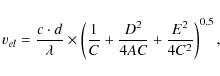
The images were flux calibrated using the observed standard stars. The
surface brightness of the scattered light was calculated by determining
the scale factor
![]() that converts
that converts
![]() to
to
![]() .
The scale factor was calculated as
.
The scale factor was calculated as
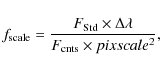
where
3.2 Polarisation with EFOSC2
Several different sources may contribute to the measured polarised
light: the central star, stellar light scattered in the interstellar
medium, the sky, and the telescope and instruments, as well as
polarised light from the sky background. In the following analysis,
however, we assume that the stellar light is unpolarised. This is
confirmed by BVRI polarimetry studies of variable stars, setting a strong upper limit on the polarisation of the stars (![]() ,
Raveendran 1991).
Further, the relative proximity of U Ant suggests a negligible
contribution to the observed polarisation from the interstellar medium.
The observations were made just after new moon, limiting the amount of
polarised light due to the background. Finally, although time
limitations prevented us from taking images of polarimetric standards
in order to characterise the effects of the telescope and the
instrument, there are no indications that these might introduce any
significant polarisation in the observations. This was confirmed by
GD2003, who observed template stars using the same instrumental set-up.
They found no polarisation in the regions where the scattered stellar
light was detected.
,
Raveendran 1991).
Further, the relative proximity of U Ant suggests a negligible
contribution to the observed polarisation from the interstellar medium.
The observations were made just after new moon, limiting the amount of
polarised light due to the background. Finally, although time
limitations prevented us from taking images of polarimetric standards
in order to characterise the effects of the telescope and the
instrument, there are no indications that these might introduce any
significant polarisation in the observations. This was confirmed by
GD2003, who observed template stars using the same instrumental set-up.
They found no polarisation in the regions where the scattered stellar
light was detected.
Therefore, assuming that all the polarised light is due to scattering
in the circumstellar environment of the star, the Stokes parameters for
the shell emission are given by
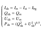
where Im,
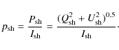
The Stokes' parameters can now be determined in a straightforward way from the observed images
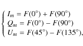
where F indicates the frames taken at the different polarisation angles.
![\begin{figure}
\par\includegraphics[width=8cm,clip]{13376f1a.eps}
\end{figure}](/articles/aa/full_html/2010/03/aa13376-09/img45.png)
|
Figure 1: Azimuthally averaged radial profiles (AARPs) in the F59 filter of U Ant (solid line), the template star (dashed line), and a moffat function fitted to the data (dotted line). |
| Open with DEXTER | |
The most difficult task is the determination of the total intensity in the circumstellar shell
![]() .
The stellar psf, due to light scattered in the Earth's atmosphere and
the telescope, was first removed by scaling and subtracting an image of
a template star with the same spectral characteristics as U Ant.
This requires an exact alignment of the template and source stars,
as well as a very well-defined and ``clean'' template psf.
Unfortunately, the images of the template star contained a large number
of back- and foreground stars, making it impossible to cleanly subtract
the stellar psf. We therefore fitted Moffat profiles (Moffat 1969)
to the azimuthally averaged radial profiles (AARPs) of the brightness
distributions in the U Ant template star images (the latter
were averaged over the same position angles as in the U Ant
images). The Moffat profile is described by
.
The stellar psf, due to light scattered in the Earth's atmosphere and
the telescope, was first removed by scaling and subtracting an image of
a template star with the same spectral characteristics as U Ant.
This requires an exact alignment of the template and source stars,
as well as a very well-defined and ``clean'' template psf.
Unfortunately, the images of the template star contained a large number
of back- and foreground stars, making it impossible to cleanly subtract
the stellar psf. We therefore fitted Moffat profiles (Moffat 1969)
to the azimuthally averaged radial profiles (AARPs) of the brightness
distributions in the U Ant template star images (the latter
were averaged over the same position angles as in the U Ant
images). The Moffat profile is described by
![\begin{displaymath}%
I=I_0\times \left[1+\left({{r}\over{r_0}}\right)^2\right]^{-b},
\end{displaymath}](/articles/aa/full_html/2010/03/aa13376-09/img46.png)
where I0 is the maximum intensity, r the distance from the centre, and r0 the width of the profile. The exponent b determines how quickly the profile decreases. The psf is assumed to be circularly symmetric. The best-fit Moffat profile is determined manually taking both the U Ant and the template star profiles into consideration. The exponent, width, and maximum intensity of the Moffat profile were adjusted until it matched the U Ant observations close to the edge of the occulting mask (
The uncertainty of the template subtraction and other instrumental
effects significantly reduce the quality of the information in the
central parts of the images. As reliable measurements are not
possible, this region is blanked out in the images by a mask with
a 20
![]() radius. The dominant diffraction spikes due to the spiders were blanked out as well.
radius. The dominant diffraction spikes due to the spiders were blanked out as well.
3.3 EMMI echelle spectra
The spectroscopic images from EMMI were reduced using standard tasks in IRAF for flat fielding and bias subtraction. The spectrum obtained on the CCD is usually significantly curved when a long slit is used. This curvature is not necessarily constant over the entire CCD, and the spectrum needs to be carefully straightened. This was done using different tasks for long-slit spectroscopy in the IRAF noao.twospec.longslit package.
Due to the use of order-sorting filters instead of a cross disperser,
the determination of the dispersion in the EMMI data proved to be
problematic. In fact, three lines were visible in the F77 data,
although at most two (the two resonance lines) were expected,
indicating an order overlap. This was confirmed by examining the
profiles of the flat-field images along the dispersion axis, showing
that the F77 filter has its centre in the region between two
orders. Hence, the lines observed in the F77 filter show two
orders of the 769.9 nm line, and one order of the 766.5 nm
line. Although the dispersion usually does not vary much between
neighbouring orders in echelle spectra, the widths of the ellipses
(due to the expansion of the shell) in the two orders differs
significantly (by
![]() ).
The widths of the 769.9 nm and 766.5 nm lines in the same
order differ as well, indicating that the dispersion varies also
within one order. The two orders lie close to the edge of the CCD,
hence the dispersion may be affected by the optics of the instrumental
setup. A careful determination of the dispersion at the position
of the lines is therefore extremely important for a correct
determination of the kinematical properties.
).
The widths of the 769.9 nm and 766.5 nm lines in the same
order differ as well, indicating that the dispersion varies also
within one order. The two orders lie close to the edge of the CCD,
hence the dispersion may be affected by the optics of the instrumental
setup. A careful determination of the dispersion at the position
of the lines is therefore extremely important for a correct
determination of the kinematical properties.
The identification of spectral lines in the calibration spectra is nearly impossible when different orders overlap. However, although the images were taken well offset from the central star, stellar light scattered in the atmosphere and the instrument is still projected onto the slit. This, in principle unfortunate fact, made it possible to compare the stellar spectrum with an archived and wavelength-calibrated spectrum of a star of similar spectral type (the carbon star HD 20234), resulting in a good dispersion calibration.
The centre of the F59 filter lies close to the centre of one order, hence there is little or no order overlap in this filter. In this case, however, the calibration spectrum is dominated by one very strong line, making it impossible to identify other lines in the spectrum for a wavelength calibration. (In the case of ordinary echelle spectra, this does not create a problem, as the dispersion solution is extrapolated from the calibration in neighbouring orders.) The atmospheric Na resonance lines are clearly visible in the data though, and the comparison with a spectrum of a star of similar spectral type leads to a good dispersion solution also in this filter.
3.4 APEX CO radio line data
The on-the-fly data was reduced using CLASS![]() .
The entire data set was inspected manually, and about 80 spectra
out of 735 were dropped because of various anomalies. The
baselines in the remaining data were relatively stable, and only second
order polynomial fits were subtracted. Once we had a consistent data
set, the remaining spectra were averaged per position, using a weight
determined by the noise level, to a grid-spacing of 8
.
The entire data set was inspected manually, and about 80 spectra
out of 735 were dropped because of various anomalies. The
baselines in the remaining data were relatively stable, and only second
order polynomial fits were subtracted. Once we had a consistent data
set, the remaining spectra were averaged per position, using a weight
determined by the noise level, to a grid-spacing of 8
![]() .
Figure 2 shows the map of the velocity-integrated intensity, in a
.
Figure 2 shows the map of the velocity-integrated intensity, in a ![]() 5 km s-1
interval centered on the systemic velocity (this range is chosen
since it gives the best view of the shell position, considering also
the signal-to-noise ratio), in the second quadrant of the detached
shell. The shell can clearly be seen and its location is consistent
with the results from the CO(J = 1-0 and 2-1) maps reported by Olofsson et al. (1996).
Emission from the present-day mass loss is also visible. The decrease
of emission to the north and west is an artefact due to the limited map
size in combination with the beam size.
5 km s-1
interval centered on the systemic velocity (this range is chosen
since it gives the best view of the shell position, considering also
the signal-to-noise ratio), in the second quadrant of the detached
shell. The shell can clearly be seen and its location is consistent
with the results from the CO(J = 1-0 and 2-1) maps reported by Olofsson et al. (1996).
Emission from the present-day mass loss is also visible. The decrease
of emission to the north and west is an artefact due to the limited map
size in combination with the beam size.
![\begin{figure}
\par\includegraphics[width=8.5cm,clip]{13376f2a.eps}
\end{figure}](/articles/aa/full_html/2010/03/aa13376-09/img50.png)
|
Figure 2:
A CO(J = 3-2) velocity-integrated intensity map in a |
| Open with DEXTER | |
4 Results
4.1 Review of previous results
CO radio line observations of U Ant show a, not so common,
highly double-peaked profile. This was interpreted as emission from a
geometrically thin, detached gas shell around U Ant, an
interpretation confirmed by mapping the CO line emission (Olofsson
et al. 1996). Models show that the CO data is consistent with a detached shell of gas with a radius of
![]()
![]() (Schöier et al. 2005).
GD2001 and GD2003 observed the circumstellar environment of U Ant
in both direct imaging and polarisation mode through two filters
covering the Na and K resonance lines (the F59 and
F77 filters, respectively). They introduced four shells, at
(Schöier et al. 2005).
GD2001 and GD2003 observed the circumstellar environment of U Ant
in both direct imaging and polarisation mode through two filters
covering the Na and K resonance lines (the F59 and
F77 filters, respectively). They introduced four shells, at ![]() 25
25
![]() ,
37
,
37
![]() ,
43
,
43
![]() ,
and 46
,
and 46
![]() (shells 1 to 4, respectively). Shells 1 and 2 were
only tentative. Shell 4 was introduced tentatively in GD2001, and
it was confirmed in GD2003. The polarisation measurements of GD2003
indicate a separation of the dust and the gas, shell 4 consisting
of mainly dust while shell 3 is dominated by gas. The
CO radio emission lines most likely come from shell 3.
Figure 3
shows the positions of the different shells. The vertical lines show
the positions of the slit in the EMMI data presented here.
Izumiura et al. (1997) reported the detection of two dust shells in IRAS images at 60
(shells 1 to 4, respectively). Shells 1 and 2 were
only tentative. Shell 4 was introduced tentatively in GD2001, and
it was confirmed in GD2003. The polarisation measurements of GD2003
indicate a separation of the dust and the gas, shell 4 consisting
of mainly dust while shell 3 is dominated by gas. The
CO radio emission lines most likely come from shell 3.
Figure 3
shows the positions of the different shells. The vertical lines show
the positions of the slit in the EMMI data presented here.
Izumiura et al. (1997) reported the detection of two dust shells in IRAS images at 60 ![]() and 100
and 100 ![]() m. They processed the images to obtain higher-resolution IRAS (HIRAS) images and derived shell radii of
m. They processed the images to obtain higher-resolution IRAS (HIRAS) images and derived shell radii of
![]() and
and
![]() ,
respectively. The shell at 3
,
respectively. The shell at 3![]() is outside our field of view, and will not be considered further.
is outside our field of view, and will not be considered further.
In light of these previous results, we present the results of our new data in the following sections, describing the images in polarised, scattered light from EFOSC2 (Sect. 4.2) and the derivation of shell fluxes, radii and widths (Sect. 4.4). The expansion velocity of shell 3 is determined from the EMMI data (Sect. 4.5). The different contributions to the scattered light from the dust and gas are estimated (Sect. 4.6) and the new CO data from APEX is modelled (Sect. 4.7). Finally, the dust masses in the individual shells are determined (Sect. 4.8).
![\begin{figure}
\par\includegraphics[width=8cm,clip]{13376f3a.eps}
\end{figure}](/articles/aa/full_html/2010/03/aa13376-09/img55.png)
|
Figure 3: A schematic drawing showing the positions of shells around U Ant as derived in GD2001 and GD2003 (shells 1 to 4 in order of increasing size; shells 1 and 2 were tentatively introduced). The vertical lines indicate the positions of the slit in the EMMI observations presented here. |
| Open with DEXTER | |
4.2 Images and radial profiles of the scattered light
![\begin{figure}
\par\includegraphics[width=5.5cm,clip]{13376f4a.eps}\hspace*{5mm}...
....eps}\hspace*{5mm}
\includegraphics[width=5.5cm,clip]{13376f4f.eps}
\end{figure}](/articles/aa/full_html/2010/03/aa13376-09/img56.png)
|
Figure 4:
The results of the EFOSC2 observations of U Ant. Top row, left to right: the total intensity (
|
| Open with DEXTER | |
![\begin{figure}
\par\includegraphics[width=5.5cm,clip]{13376f5a.eps}\hspace*{5mm}...
....eps}\hspace*{5mm}
\includegraphics[width=5.5cm,clip]{13376f5i.eps}
\end{figure}](/articles/aa/full_html/2010/03/aa13376-09/img57.png)
|
Figure 5:
AARPs from the EFOSC2 observations of U Ant. Top row, left to right: the total intensity (
|
| Open with DEXTER | |
Figure 4 shows the total flux,
![]() ,
and polarised flux,
,
and polarised flux,
![]() ,
images in the Str-y, F59, and H
,
images in the Str-y, F59, and H![]() filters. AARPs of the
filters. AARPs of the
![]() ,
,
![]() ,
and the polarisation degree,
,
and the polarisation degree,
![]() ,
are shown in Fig. 5.
,
are shown in Fig. 5.
The morphology in the H![]() and Str-y
and Str-y
![]() images differs significantly from that in the F59 filter. The former both show a circular disk of
images differs significantly from that in the F59 filter. The former both show a circular disk of ![]() 50
50
![]() radius. The
radius. The
![]() AARPs in both filters show that the intensity remains relatively constant out to a radius of
AARPs in both filters show that the intensity remains relatively constant out to a radius of ![]() 50
50
![]() followed by a tail of declining intensity. GD2003 showed that such a
brightness distribution is consistent with scattering of stellar light
in a detached shell of dust, assuming that the dust has a preferential
scattering efficiency in the forward direction. The irregularities in
the AARPs are likely due to a few bright arcs present in the images
closer to the star. However, a small peak at
followed by a tail of declining intensity. GD2003 showed that such a
brightness distribution is consistent with scattering of stellar light
in a detached shell of dust, assuming that the dust has a preferential
scattering efficiency in the forward direction. The irregularities in
the AARPs are likely due to a few bright arcs present in the images
closer to the star. However, a small peak at ![]() 43
43
![]() indicates the presence of an additional shell, and an extended arc at
this distance from the star is clearly seen in both filters in the
south-east quadrant.
indicates the presence of an additional shell, and an extended arc at
this distance from the star is clearly seen in both filters in the
south-east quadrant.
The
![]() AARP of the F59 image shows a much more pronounced peak at
AARP of the F59 image shows a much more pronounced peak at ![]() 43
43
![]() ,
while the tail at
,
while the tail at ![]() 48
48
![]() is
relatively weak. Since the F59 filter may contain a contribution
from stellar light scattered in the NaD resonance lines, while the
H
is
relatively weak. Since the F59 filter may contain a contribution
from stellar light scattered in the NaD resonance lines, while the
H![]() and Str-y filters are dominated by dust scattered light, this
confirms the results by GD2003, where shell 3 is dominated by
line scattering, while shell 4 is dominated by dust scattering.
and Str-y filters are dominated by dust scattered light, this
confirms the results by GD2003, where shell 3 is dominated by
line scattering, while shell 4 is dominated by dust scattering.
Only light that is scattered at an angle of ![]() 90
90![]() will be strongly polarised. The polarisation due to the circumstellar
medium will hence be strongest in the plane of the sky that goes
through the star. Detached, spherical shells appear as ring-like
structures in such images, directly revealing the spatial structure of
the shells. The images in the polarised flux
will be strongly polarised. The polarisation due to the circumstellar
medium will hence be strongest in the plane of the sky that goes
through the star. Detached, spherical shells appear as ring-like
structures in such images, directly revealing the spatial structure of
the shells. The images in the polarised flux
![]() in all filters clearly show a nearly perfect circular geometry. The corresponding AARPs show the presence of two shells at
in all filters clearly show a nearly perfect circular geometry. The corresponding AARPs show the presence of two shells at ![]() 43
43
![]() and
and ![]() 48
48
![]() ,
corresponding to the positions of shells 3 and 4
in GD2003, but GD2003 did not detect shell 3 in the
polarised light images. These AARPs make it possible to determine the
locations and the widths of shells 3 and 4. Fits to the AARPs
of the
,
corresponding to the positions of shells 3 and 4
in GD2003, but GD2003 did not detect shell 3 in the
polarised light images. These AARPs make it possible to determine the
locations and the widths of shells 3 and 4. Fits to the AARPs
of the
![]() images in all filters show that the total polarised flux is dominated by shell 4 (see Sect. 4.4). Shell 4 also clearly dominates the AARPs of the
images in all filters show that the total polarised flux is dominated by shell 4 (see Sect. 4.4). Shell 4 also clearly dominates the AARPs of the
![]() images, the degree of polarisation reaching a maximum of 25-30% in all three filters at a radius of
images, the degree of polarisation reaching a maximum of 25-30% in all three filters at a radius of ![]() 50
50
![]() ,
confirming that shell 4 is dominated by stellar light scattered by dust. Since
,
confirming that shell 4 is dominated by stellar light scattered by dust. Since
![]() is derived
is derived
![]() /
/
![]() ,
the outer parts (where
,
the outer parts (where
![]() and
and
![]() )
become less reliable. Hence, the picture of a shell of gas at the
position of shell 3 containing a small amount of dust, and a
detached shell dominated by dust with almost no gas at the position of
shell 4 is strengthened.
)
become less reliable. Hence, the picture of a shell of gas at the
position of shell 3 containing a small amount of dust, and a
detached shell dominated by dust with almost no gas at the position of
shell 4 is strengthened.
Structure inside shell 3 is apparent in the F59 image (but not in the
others, including the F77 image of GD2003). The positions of the
peaks in the AARP are consistent with shells 1 and 2 in
GD2001 at 25
![]() and 37
and 37
![]() .
It is not clear, however, whether the observed structure is due to
clumpy structures in shells 3 and/or 4, or due to additional
detached shells closer to the star, see Sect. 5.1.1.
.
It is not clear, however, whether the observed structure is due to
clumpy structures in shells 3 and/or 4, or due to additional
detached shells closer to the star, see Sect. 5.1.1.
4.3 Scattering in detached gas and dust shells
In order to understand the origin of detached shells, it is important to accurately determine their physical parameters, such as e.g. shell radius and width, and its density distribution and possible clumpiness. Any determination of physical properties of the shells based on the data presented here requires the proper treatment of the scattering agent properties. For an individual dust grain these are affected by, e.g., the grain composition, size, and shape. The observed brightness distributions (due to scattering by a large number of grains) are affected by the grain size distribution, the density distribution within the shell, and the size and width of the shell.
The scattering by the grains can be calculated using Mie theory,
given the optical constants of the grains. If the grain size is
small compared to the scattering wavelength (
![]() ),
the condition for Rayleigh scattering is fulfilled and the scattering
can be assumed to be isotropic. However, typical grain sizes are
),
the condition for Rayleigh scattering is fulfilled and the scattering
can be assumed to be isotropic. However, typical grain sizes are ![]() 0.1
0.1 ![]() m,
i.e. comparable to the wavelengths in our data, and asymmetric
scattering becomes important. In order to determine the amount of
scattering in a particular direction (i.e. the probability for
scattering in a direction
m,
i.e. comparable to the wavelengths in our data, and asymmetric
scattering becomes important. In order to determine the amount of
scattering in a particular direction (i.e. the probability for
scattering in a direction ![]() with respect to the forward direction), we use an analytical expression
(based on light scattered in the interstellar medium; Henyey &
Greenstein 1941)
with respect to the forward direction), we use an analytical expression
(based on light scattered in the interstellar medium; Henyey &
Greenstein 1941)
where g is the scattering asymmetry parameter defined as
where

![\begin{figure}
\par\includegraphics[width=5.5cm,clip]{13376f6a.eps}\hspace*{5mm}...
....eps}\hspace*{5mm}
\includegraphics[width=5.5cm,clip]{13376f6c.eps}
\end{figure}](/articles/aa/full_html/2010/03/aa13376-09/img67.png)
|
Figure 6:
Left: the scattering efficiency
|
| Open with DEXTER | |
Table 2:
The results of decomposing the
![]() AARP data into shell brightness distributions.
AARP data into shell brightness distributions.
Table 3:
The results of decomposing the
![]() AARP data into shell brightness distributions.
AARP data into shell brightness distributions.
The left panel of Fig. 6 shows the scattering efficiency
![]() of dust grains and the scattering parameter g vs. wavelength for amorphous carbon grains (Suh 2000) assuming spherical grains with radii of 0.1
of dust grains and the scattering parameter g vs. wavelength for amorphous carbon grains (Suh 2000) assuming spherical grains with radii of 0.1 ![]() m. Equation (6)
can then be used to derive radial brightness distributions for
different wavelengths assuming single scattering. The middle panel of
Fig. 6 shows the expected brightness distributions for optically thin scattering by dust in a detached shell located at R = 48
m. Equation (6)
can then be used to derive radial brightness distributions for
different wavelengths assuming single scattering. The middle panel of
Fig. 6 shows the expected brightness distributions for optically thin scattering by dust in a detached shell located at R = 48
![]() from the star. They are given for complete isotropic scattering (g = 0) and for the calculated g
for the respective filters. The density distribution of the detached
shell along the radial direction is assumed to follow a Gaussian
distribution with a FWHM of
from the star. They are given for complete isotropic scattering (g = 0) and for the calculated g
for the respective filters. The density distribution of the detached
shell along the radial direction is assumed to follow a Gaussian
distribution with a FWHM of
![]()
![]() peaking at R. The grains have a constant size of
peaking at R. The grains have a constant size of ![]() m. The right panel of Fig. 6 shows the corresponding profiles for the polarised light.
m. The right panel of Fig. 6 shows the corresponding profiles for the polarised light.
For all cases the limb brightening due to the narrow shell is apparent at
![]()
![]() (hereafter referred to as the ``peak''). However, as forward
scattering becomes more effective for shorter wavelengths, the
brightness profile at line of sights closer to the star increases
compared to the peak intensity. Note that the amount of forward
scattering does not have an effect on the position of the peak or the
sharp decrease at larger radii. However, the density distribution
within the shell affects the shape of the peak. A sharp inner edge
moves the position of the peak somewhat closer to the star, while a
sharp outer edge leads to a sharper decline at large radii. The decline
in brightness at large radii follows to good approximation
a Gaussian distribution and it gives reasonable estimates of the
radius and width of the shell (Mauron & Huggins 2000). However, fitting a Gaussian distribution to the peak and the tail results in a slightly underestimated radius R (by
(hereafter referred to as the ``peak''). However, as forward
scattering becomes more effective for shorter wavelengths, the
brightness profile at line of sights closer to the star increases
compared to the peak intensity. Note that the amount of forward
scattering does not have an effect on the position of the peak or the
sharp decrease at larger radii. However, the density distribution
within the shell affects the shape of the peak. A sharp inner edge
moves the position of the peak somewhat closer to the star, while a
sharp outer edge leads to a sharper decline at large radii. The decline
in brightness at large radii follows to good approximation
a Gaussian distribution and it gives reasonable estimates of the
radius and width of the shell (Mauron & Huggins 2000). However, fitting a Gaussian distribution to the peak and the tail results in a slightly underestimated radius R (by ![]() 8%) and an overestimated FWHM of the shell (by
8%) and an overestimated FWHM of the shell (by ![]() 20%).
Hence, the detailed grain size distribution and the density
distribution across the shell are the main uncertainties in determining
the shell radius and width from the observed brightness distributions.
20%).
Hence, the detailed grain size distribution and the density
distribution across the shell are the main uncertainties in determining
the shell radius and width from the observed brightness distributions.
In the case of line scattering we use Eq. (6) with g = 0 for calculating the brightness distribution.
4.4 Decomposition of the AARPs
In order to derive quantitative results for the individual shells it
is necessary to decompose the AARPs obtained from the observed images.
The images in polarised light best show the spatial structure of the
dust, and we use Eqs. (6) and (8) to derive theoretical AARPs for the polarised scattered light. The scattering asymmetry parameter g is determined for each filter using Mie theory and assuming spherical, 0.1 ![]() m sized carbon grains (Suh 2000).
A Gaussian density distribution of the dust as described above is
assumed. The model distributions are fit to the peaks in the
m sized carbon grains (Suh 2000).
A Gaussian density distribution of the dust as described above is
assumed. The model distributions are fit to the peaks in the
![]() AARPs, hence determining the radius and widths of shells 3 and 4. Equation (6) is then used to calculate model profiles of the total intensity
AARPs, hence determining the radius and widths of shells 3 and 4. Equation (6) is then used to calculate model profiles of the total intensity
![]() .
In the F59 filter shell 3 is assumed to be dominated by
scattering in lines, and hence isotropic scattering is assumed in this
filter (g = 0). The dust contribution to
.
In the F59 filter shell 3 is assumed to be dominated by
scattering in lines, and hence isotropic scattering is assumed in this
filter (g = 0). The dust contribution to
![]() from shell 3 in this filter is neglected. The dotted lines in Fig. 5 show the individual brightness distributions. Tables 2 and 3
show the results of fitting the brightness distributions to the
polarised and total flux AARPs, respectively. For the latter, the shell
radii and sizes determined from the polarisation data are used. Hence,
we confirm the detection of detached shells at 43
from shell 3 in this filter is neglected. The dotted lines in Fig. 5 show the individual brightness distributions. Tables 2 and 3
show the results of fitting the brightness distributions to the
polarised and total flux AARPs, respectively. For the latter, the shell
radii and sizes determined from the polarisation data are used. Hence,
we confirm the detection of detached shells at 43
![]() (shell 3) and 50
(shell 3) and 50
![]() (shell 4) from the star. The width of shell 3 is
(shell 4) from the star. The width of shell 3 is ![]() 2
2
![]() 2, while shell 4 is a factor of 3 broader. The results for the F77 filter in Table 3 are taken from GD2003. The fluxes for the individual shells in Table 3
are derived by summing the model brightness distributions over all
angles. The total fluxes for all shells are calculated by summing the
observed profiles over all angles (labelled ``total''
in Table 3).
2, while shell 4 is a factor of 3 broader. The results for the F77 filter in Table 3 are taken from GD2003. The fluxes for the individual shells in Table 3
are derived by summing the model brightness distributions over all
angles. The total fluxes for all shells are calculated by summing the
observed profiles over all angles (labelled ``total''
in Table 3).
In all measurements probing the contribution to the flux from dust
scattered light (i.e. the polarisation measurements and the
![]() images in the Str-y and H
images in the Str-y and H![]() filters),
shell 4 clearly dominates over shell 3. The contribution to
the total flux from shell 3 is only comparable to that from
shell 4 in the
filters),
shell 4 clearly dominates over shell 3. The contribution to
the total flux from shell 3 is only comparable to that from
shell 4 in the
![]() images
in the F59 filter. This is likely due to the added contribution of
line scattered light in shell 3 in this filter.
images
in the F59 filter. This is likely due to the added contribution of
line scattered light in shell 3 in this filter.
The theoretical brightness distributions do not perfectly fit
the observed AARPs. Artefacts in the images (e.g., diffraction
spikes), the uncertainty due to the psf subtraction, and a possible
clumpy structure in the detached shells are likely to affect the AARPs,
in particular in the inner parts of the images. The assumption of
a constant grain-size in the model AARPs and a Gaussian density
distribution across the shells also affects the model brightness
distributions. The gradual decline at larger radii could also be a
kinematic effect, e.g., due to grains of different size travelling
at different velocities. The fit to the
![]() AARP
in the F59 filter is particularly poor. This is partly due to the
presence of structures inside shell 3, but there is most likely
also an effect of the NaD line scattering being, at least
partially, optically thick (see below). Also, the FWHM of
shell 3 in the
AARP
in the F59 filter is particularly poor. This is partly due to the
presence of structures inside shell 3, but there is most likely
also an effect of the NaD line scattering being, at least
partially, optically thick (see below). Also, the FWHM of
shell 3 in the
![]() AARP seems to be wider than the one determined from the
AARP seems to be wider than the one determined from the
![]() AARP. This is likely due to the small amount of dust present in shell 3.
AARP. This is likely due to the small amount of dust present in shell 3.
![\begin{figure}
\par\includegraphics[width=8.8cm,clip]{13376f7a.eps}
\end{figure}](/articles/aa/full_html/2010/03/aa13376-09/img81.png)
|
Figure 7:
EMMI long-slit spectra towards U Ant showing the
NaD resonance lines. The doublet lines are combined in order to
increase the signal-to-noise ratio. The slit is offset from the star by
15
|
| Open with DEXTER | |
![\begin{figure}
\par\includegraphics[width=8.8cm,clip]{13376f8a.eps}
\end{figure}](/articles/aa/full_html/2010/03/aa13376-09/img82.png)
|
Figure 8: Same as Fig. 7 but for the KI resonance line at 769.9 nm. |
| Open with DEXTER | |
Table 4: The results of the EMMI data.
4.5 Kinematic and spatial information from the EMMI data
Examples of the long-slit NaD and KI line data taken with EMMI are shown in Figs. 7 and 8,
respectively. The ellipse-like shape of the lines due to the expansion
of a geometrically, essentially spherical thin circumstellar shell can
clearly be seen. As mentioned above, the NaD lines show a
more complicated morphology, revealing additional structure closer to
the star. However, we focus the analysis on the dominating shell.
Ellipses were fit to the data (obtained by making cuts along the
dispersion axis and fitting Gaussian profiles to the line intensity
distribution) using the conical representation of an ellipse
where x and y are the points of the ellipse along the spatial and dispersion axes, respectively. The parameters A-E were determined by fitting the ellipse to the centres of the Gaussian profiles using a least-squares-fit method. The length
where c is the speed of light, d the dispersion in
The EMMI data is dominated by scattering in a shell with a radius of ![]() 40
40
![]() and a width of
and a width of ![]() 3
3
![]() ,
that expands at a velocity of 19.5
,
that expands at a velocity of 19.5
![]() .
Although the fit of an ellipse to the data is generally very good,
effects due to the physical width of the slit, and the resolved spatial
structure of the shell result in deviations from a perfect ellipse at
the end points. This causes the measured size of the shell to be
systematically smaller (by
.
Although the fit of an ellipse to the data is generally very good,
effects due to the physical width of the slit, and the resolved spatial
structure of the shell result in deviations from a perfect ellipse at
the end points. This causes the measured size of the shell to be
systematically smaller (by ![]() 2
2
![]() )
than suggested by the peaks measured directly in the data. Taking this
into consideration, the results are fully consistent with the EFOSC2
and CO radio line data on shell 3. The expansion velocity
determined from the resonance line data is in excellent agreement with
that obtained from models of the CO emission lines, 19.0
)
than suggested by the peaks measured directly in the data. Taking this
into consideration, the results are fully consistent with the EFOSC2
and CO radio line data on shell 3. The expansion velocity
determined from the resonance line data is in excellent agreement with
that obtained from models of the CO emission lines, 19.0
![]() (Schöier et al. 2005).
(Schöier et al. 2005).
The brightness of the red-shifted side of the shell (i.e., the rear part as seen from Earth) is clearly brighter than the front in the NaD data. The same effect can be seen to a lesser extent in the KI data. This most likely is an optical depth effect. A higher optical depth in the NaD lines leads to increased reflection of the light on the red-shifted side of the shell, while more of the light is scattered away from the line of sight on the blue-shifted side.
Finally, the EMMI data taken through the F59 filter also shows
structures inside shell 3 in the NaD line, but ellipses are
not apparent (see Fig. 7). A cut along the spatial axis at the systemic velocity reveals peaks also at 23
![]() and 34
and 34
![]() (corrected for projection effects), at the positions of the
tentative shells 1 and 2. This structure is not seen in the
F77 filter data, i.e., in the KI line.
(corrected for projection effects), at the positions of the
tentative shells 1 and 2. This structure is not seen in the
F77 filter data, i.e., in the KI line.
4.6 Line vs. dust scattering
Previous observations of scattered light in the detached shells
around U Ant (GD2001 and GD2003) were made in filters containing
strong resonance lines (except for a tentative detection of
shell 4 in a Strömgren b filter at 469.0 nm). Since the
widths of the lines are much smaller than the filter width, such
observations also contain stellar light scattered by dust, and it is
difficult to disentangle the contributions from the different
scattering agents. Observations of polarised light mainly measure light
scattered by dust (resonance line scattering only accounting for up to
![]() of the polarised light; Loskutov & Ivanov 2007),
and observations with filters that contain no lines make it possible to
determine the amount of dust-scattered light, and, together with
observations in the ``line''-filters, the amount of line-scattered
light.
of the polarised light; Loskutov & Ivanov 2007),
and observations with filters that contain no lines make it possible to
determine the amount of dust-scattered light, and, together with
observations in the ``line''-filters, the amount of line-scattered
light.
Table 3 gives the flux densities in the different filters. Through linear inter- and extrapolatation of the data in the H![]() and
Str-y filters (assumed to contain contributions only from dust),
it is possible to estimate the fractions of flux in the F59 and
F77 filters that are due to dust. The result is that
and
Str-y filters (assumed to contain contributions only from dust),
it is possible to estimate the fractions of flux in the F59 and
F77 filters that are due to dust. The result is that ![]() 43% and
43% and ![]() 50%
of the total fluxes in the F59 and F77 filters, respectively, can
be attributed to scattering in dust. The total polarised flux is
50%
of the total fluxes in the F59 and F77 filters, respectively, can
be attributed to scattering in dust. The total polarised flux is ![]() 7 times higher in shell 4 than in shell 3 in all filters (Table 2),
showing that the dominant contribution to the dust scattered light must
come from shell 4. This is in agreement with the results in the
polarisation degree, reaching its maximum (
7 times higher in shell 4 than in shell 3 in all filters (Table 2),
showing that the dominant contribution to the dust scattered light must
come from shell 4. This is in agreement with the results in the
polarisation degree, reaching its maximum (
![]() )
at the position of shell 4. Hence, we can conclude that
shell 3 is dominated by gas (and line scattering clearly dominates
in the F59 (
)
at the position of shell 4. Hence, we can conclude that
shell 3 is dominated by gas (and line scattering clearly dominates
in the F59 (![]() 81% of the total flux) and F77 (
81% of the total flux) and F77 (![]() 97% of the total flux) filter images, while dust dominates in shell 4.
97% of the total flux) filter images, while dust dominates in shell 4.
4.7 The CO shell
Compared to the CO(J = 1-0 and 2-1) data in Olofsson et al. (1996), the APEX data presented here provides a higher angular resolution (18
![]() beamwidth). Figure 9 shows the intensity (averaged over the central 10 km s-1) AARP of the new CO(J = 3-2)
data. The emissions from the shell and the present-day mass-loss wind
are clearly separated. We here model the new CO(J = 3-2)
data to show that the CO shell coincides with shell 3. The
models are based on the best-fit model presented by Schöier et al.
(2005), slightly adjusted
to fit the new APEX data. The code used in the CO line
modelling is described in Schöier & Olofsson (2001).
beamwidth). Figure 9 shows the intensity (averaged over the central 10 km s-1) AARP of the new CO(J = 3-2)
data. The emissions from the shell and the present-day mass-loss wind
are clearly separated. We here model the new CO(J = 3-2)
data to show that the CO shell coincides with shell 3. The
models are based on the best-fit model presented by Schöier et al.
(2005), slightly adjusted
to fit the new APEX data. The code used in the CO line
modelling is described in Schöier & Olofsson (2001).
Following Schöier et al. (2005) we adopt a shell width of 1.6 ![]() 1016 cm (this corresponds to 2
1016 cm (this corresponds to 2
![]() 6
at the distance of U Ant, i.e., close to the shell width as
estimated from the line scattering data, which is much smaller than the
angular resolution of the APEX CO line data). The kinetic
temperature in the shell is set to 350 K. The density in the shell
is assumed to be constant and defined by the gas shell mass
(see below). The expansion velocity of the shell is estimated to
be 19.0
6
at the distance of U Ant, i.e., close to the shell width as
estimated from the line scattering data, which is much smaller than the
angular resolution of the APEX CO line data). The kinetic
temperature in the shell is set to 350 K. The density in the shell
is assumed to be constant and defined by the gas shell mass
(see below). The expansion velocity of the shell is estimated to
be 19.0
![]() by fitting the CO line profiles. For the present-day mass loss we use a mass-loss rate of 1.2
by fitting the CO line profiles. For the present-day mass loss we use a mass-loss rate of 1.2 ![]()
![]() .
This is about a factor of two lower than that obtained by Schöier et al. (2005). The latter is a result of an average fit to three CO lines, and the SEST CO(J = 3-2)
line is almost a factor of two stronger than the corresponding
APEX line. However, it is clear that the APEX line is
more reliably calibrated than the SEST line (SEST had a main
beam efficiency as low as 25% at 345 GHz), and we therefore
adjust the mass-loss rate to fit the APEX line. In fact,
as can be seen both in Figs. 2 and 9,
the present-day mass-loss emission is well separated from the detached
shell emission, and only contributes to the AARP in the form of
a Gaussian profile with the same width as the APEX beam.
Therefore, the main goal of the APEX data to verify the position
of the detached CO shell is not dependent on the assumption of the
present-day mass-loss rate. The stellar radiation field is a central
blackbody with a luminosity of 5800
.
This is about a factor of two lower than that obtained by Schöier et al. (2005). The latter is a result of an average fit to three CO lines, and the SEST CO(J = 3-2)
line is almost a factor of two stronger than the corresponding
APEX line. However, it is clear that the APEX line is
more reliably calibrated than the SEST line (SEST had a main
beam efficiency as low as 25% at 345 GHz), and we therefore
adjust the mass-loss rate to fit the APEX line. In fact,
as can be seen both in Figs. 2 and 9,
the present-day mass-loss emission is well separated from the detached
shell emission, and only contributes to the AARP in the form of
a Gaussian profile with the same width as the APEX beam.
Therefore, the main goal of the APEX data to verify the position
of the detached CO shell is not dependent on the assumption of the
present-day mass-loss rate. The stellar radiation field is a central
blackbody with a luminosity of 5800 ![]() and an effective temperature of 2800 K. Finally, we adjust the position of the shell to get the best fit to the CO(J = 3-2) intensity AARP. The resulting shell radius is 41
and an effective temperature of 2800 K. Finally, we adjust the position of the shell to get the best fit to the CO(J = 3-2) intensity AARP. The resulting shell radius is 41
![]() .
.
The result of the modelling is presented in the form of a model AARP in Fig. 9. The observed AARP is consistent with a model of a detached shell with a radius of 41
![]() ,
i.e., the CO shell coincides, well within the uncertainties,
with shell 3, the shell responsible for the atomic line
scattering. The H2 mass of shell 3 is estimated to be 2
,
i.e., the CO shell coincides, well within the uncertainties,
with shell 3, the shell responsible for the atomic line
scattering. The H2 mass of shell 3 is estimated to be 2 ![]()
![]() assuming a CO abundance with respect to H2 of 10-3 (see Table 5).
assuming a CO abundance with respect to H2 of 10-3 (see Table 5).
![\begin{figure}
\par\includegraphics[angle=-90,width=7.5cm,clip]{13376f9a.eps}
\end{figure}](/articles/aa/full_html/2010/03/aa13376-09/img95.png)
|
Figure 9:
AARP of the APEX CO(J = 3-2) intensity averaged over the central 10
|
| Open with DEXTER | |
4.8 The mass of the dust shell
All light scattered by dust is likely to be optically thin
(see below), and it is therefore possible to do a simple
analysis of the observational results, based on an analytical approach
described in GD2001. The ratio of the circumstellar flux over the
stellar flux is given by
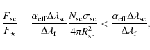
where
Assuming single-sized, spherical dust grains the number of scatterers and the scattering cross section are given by


where
The
![]() ratios are given by the observations. The model brightness distributions do not reproduce the observed
ratios are given by the observations. The model brightness distributions do not reproduce the observed
![]() AARPs well, likely due to the simplified assumption of a constant grain
size, the dust density distribution, and a clumpy medium. Hence, using
the model brightness distributions to determine
AARPs well, likely due to the simplified assumption of a constant grain
size, the dust density distribution, and a clumpy medium. Hence, using
the model brightness distributions to determine
![]() ratios
and dust masses individually for shell 3 and 4 would result
in very uncertain results. However, shell 4 dominates the
contribution from dust (Sects. 4.2 and 4.4).
We therefore assume that all dust-scattered light comes from
shell 4, and the total observed fluxes are used in determining the
dust mass (they are corrected for line scattering in the F59 and
F77 filters). The resulting dust mass of shell 4 (averaged
over all four filters) is 5
ratios
and dust masses individually for shell 3 and 4 would result
in very uncertain results. However, shell 4 dominates the
contribution from dust (Sects. 4.2 and 4.4).
We therefore assume that all dust-scattered light comes from
shell 4, and the total observed fluxes are used in determining the
dust mass (they are corrected for line scattering in the F59 and
F77 filters). The resulting dust mass of shell 4 (averaged
over all four filters) is 5 ![]() 10
10
![]() ,
Table 5. Schöier et al. (2005) modelled the thermal emission from U Ant type, and derived a dust mass of (1.3
,
Table 5. Schöier et al. (2005) modelled the thermal emission from U Ant type, and derived a dust mass of (1.3 ![]() 1.2)
1.2) ![]()
![]() at a radius of (5.1
at a radius of (5.1 ![]() 4.0)
4.0) ![]() 1017 cm,
consistent with the mass and radius derived for shell 4 here
within the considerable uncertainties. Izumiura et al. (1997) modelled two dust shells observed in high-resolution IRAS images and derived a dust mass for the inner shell of 2.2
1017 cm,
consistent with the mass and radius derived for shell 4 here
within the considerable uncertainties. Izumiura et al. (1997) modelled two dust shells observed in high-resolution IRAS images and derived a dust mass for the inner shell of 2.2 ![]()
![]() at a distance of 2.0
at a distance of 2.0 ![]() 1017 cm,
consistent with the results obtained for shell 4 here.
GD2003 derived a dust mass for shell 4 of 4
1017 cm,
consistent with the results obtained for shell 4 here.
GD2003 derived a dust mass for shell 4 of 4 ![]()
![]() ,
a factor of 10 lower than our estimate, emphasising the uncertainty in estimated dust mass.
,
a factor of 10 lower than our estimate, emphasising the uncertainty in estimated dust mass.
Table 5: Derived shell masses based on the EFOSC2 data (dust) and the APEX CO line data (gas).
4.9 The mass of the gas shell
Using the
![]() ratios for scattering in the NaD and KI lines, corrected for the
contribution from dust scattering, it is in principle possible to
estimate the gas mass of shell 3 based on the analytical approach
from GD2001 (assuming that the contribution to the observed total
fluxes from the gas is entirely due to shell 3). The requirement
of optically thin scattering sets upper limits also to the
ratios for scattering in the NaD and KI lines, corrected for the
contribution from dust scattering, it is in principle possible to
estimate the gas mass of shell 3 based on the analytical approach
from GD2001 (assuming that the contribution to the observed total
fluxes from the gas is entirely due to shell 3). The requirement
of optically thin scattering sets upper limits also to the
![]() ratios
for the KI and NaD lines. For line scattering we assume the
scattering wavelength range to be set by the turbulent velocity width.
A value typical for circumstellar environments is
ratios
for the KI and NaD lines. For line scattering we assume the
scattering wavelength range to be set by the turbulent velocity width.
A value typical for circumstellar environments is
![]() .
For the strong resonance lines
.
For the strong resonance lines
![]()
![]() 0.5 and the filter widths of the F59 and F77 filters is
0.5 and the filter widths of the F59 and F77 filters is
![]() = 5 nm, putting the upper limit to the
= 5 nm, putting the upper limit to the
![]() ratio for the KI and NaD lines at
ratio for the KI and NaD lines at ![]() 2.5
2.5 ![]() 10-4 and
10-4 and ![]() 4
4 ![]() 10-4, respectively (Eq. (12)). The observed
10-4, respectively (Eq. (12)). The observed
![]() ratio is above this limit by a factor of
ratio is above this limit by a factor of ![]() 20 in the F59 filter, while the
20 in the F59 filter, while the
![]() ratio in the F77 filter lies close to the limit (only a factor of
ratio in the F77 filter lies close to the limit (only a factor of ![]() 3 higher).
We conclude that scattering in the NaD lines is optically thick,
while scattering in the KI lines may be at least partially
optically thin. This is a likely explanation for the different
AARPs in the two filters, as well as for the difference in the
appearance in the EMMI data. Hence, it is reasonable to
expect that we can get at most a lower limit to the shell 3 gas mass
using the optically thin approximation for the line-scattered light.
3 higher).
We conclude that scattering in the NaD lines is optically thick,
while scattering in the KI lines may be at least partially
optically thin. This is a likely explanation for the different
AARPs in the two filters, as well as for the difference in the
appearance in the EMMI data. Hence, it is reasonable to
expect that we can get at most a lower limit to the shell 3 gas mass
using the optically thin approximation for the line-scattered light.
The best gas mass estimate of shell 3 is consequently obtained from the CO line modelling, 2 ![]()
![]() .
Assuming that shells 3 and 4 were created at the same time
(see below), the derived dust and gas masses give a dust-to-gas
mass ratio of
.
Assuming that shells 3 and 4 were created at the same time
(see below), the derived dust and gas masses give a dust-to-gas
mass ratio of ![]() 0.02 for the ejected material, not unreasonable for carbon-rich AGB stars.
0.02 for the ejected material, not unreasonable for carbon-rich AGB stars.
We can use the optically thin approximation and the observed
![]() ratios
(corrected for the dust contribution) to check whether the Na and
K results are consistent with the estimated shell gas mass.
Assuming a Boltzmann distribution of the population levels we have for
the number of scatterers,
ratios
(corrected for the dust contribution) to check whether the Na and
K results are consistent with the estimated shell gas mass.
Assuming a Boltzmann distribution of the population levels we have for
the number of scatterers,
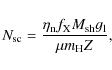
and for the line scattering cross section,
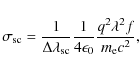
where
5 Discussion and conclusions
5.1 The identification of shells
Based on the EFOSC2 data we clearly detect two geometrically thin shells around U Ant with radii of 43
![]() and 50
and 50
![]() (shells 3
and 4, respectively). Although shell 4 is relatively weak in
the images of total scattered light, it is clearly visible in the
images of polarised light. We also confirm the tentative detection of
additional structure inside shell 3 in the F59 filter images,
a result supported by the EMMI NaD data. We proceed to
discuss the tentative shells 1 and 2, and the shells 3
and 4 in separate sections below.
(shells 3
and 4, respectively). Although shell 4 is relatively weak in
the images of total scattered light, it is clearly visible in the
images of polarised light. We also confirm the tentative detection of
additional structure inside shell 3 in the F59 filter images,
a result supported by the EMMI NaD data. We proceed to
discuss the tentative shells 1 and 2, and the shells 3
and 4 in separate sections below.
5.1.1 Shells 1 and 2
These shells were tentatively introduced by GD2003. The structures
attributed to these shells were only seen in the EFOSC2 F59 data.
The
![]() image
shows signs of arcs that may form an essentially circular shell
(shell 2). However, this putative shell is not centered on the
star. There are also arcs that seem to ``connect'' this shell and
shell 3. The presence of shell 1 was inferred only from the
image
shows signs of arcs that may form an essentially circular shell
(shell 2). However, this putative shell is not centered on the
star. There are also arcs that seem to ``connect'' this shell and
shell 3. The presence of shell 1 was inferred only from the
![]() AARP.
However, here we provide evidence for structures in the radial ranges
of shells 1 and 2 also in the EMMI NaD line data, but
these structures do not form complete (or even partial) ellipses
as expected from spherical shells centered on the star. Curiously,
these structures are not seen in any of the other data. The most
reasonable explanation for this is that the optical depth of the
NaD line scattering is high (above one) and that of the other
scattering agents is low (below one). This is consistent with the
asymmetry in the brightness between the red- and blue-shifted sides in
the EMMI data. The effect is stronger in the NaD lines,
indicating a higher optical depth than in the KI line. The spatial
resolution and the dynamic range of the CO data are not enough to
identify structures in this radial range. We conclude that there is no
strong evidence for the existence of full shells inside shell 3,
but structures do exist and their interpretation is not clear.
Whether these structures indeed are closer to the star, or whether
they are structures within the observed shells is also not clear.
AARP.
However, here we provide evidence for structures in the radial ranges
of shells 1 and 2 also in the EMMI NaD line data, but
these structures do not form complete (or even partial) ellipses
as expected from spherical shells centered on the star. Curiously,
these structures are not seen in any of the other data. The most
reasonable explanation for this is that the optical depth of the
NaD line scattering is high (above one) and that of the other
scattering agents is low (below one). This is consistent with the
asymmetry in the brightness between the red- and blue-shifted sides in
the EMMI data. The effect is stronger in the NaD lines,
indicating a higher optical depth than in the KI line. The spatial
resolution and the dynamic range of the CO data are not enough to
identify structures in this radial range. We conclude that there is no
strong evidence for the existence of full shells inside shell 3,
but structures do exist and their interpretation is not clear.
Whether these structures indeed are closer to the star, or whether
they are structures within the observed shells is also not clear.
5.1.2 Shells 3 and 4
Shells 3 and 4 are clearly present as separate entities in the polarisation data at radii of ![]() 43
43
![]() and 50
and 50
![]() ,
respectively. In the
,
respectively. In the
![]() images
shells 3 and 4 have a large degree of circular symmetry, with
slight variations in the intensity indicating a somewhat clumpy
structure. There is a gap in shells 3 and 4 in the
north-eastern corner of the polarised images, however, this is
likely due to artefacts in the images, rather than a gap in the density
distribution in the shells. The single-dish CO radio observations
do not resolve individual shells, nor do they indicate a multiple-shell
structure. However, there are several indications that the CO line
emission comes predominantly from shell 3 (Sect. 4.7). In addition, there is a ``hole'' in the south-western quadrant in the CO maps (Olofsson et al. 1996)
and this is seen also in the F59 and F77 images. Based on the flux
densities in the different filters and the polarisation data,
it is clear that shell 4 essentially consists of only dust,
while shell 3 is dominated by gas.
images
shells 3 and 4 have a large degree of circular symmetry, with
slight variations in the intensity indicating a somewhat clumpy
structure. There is a gap in shells 3 and 4 in the
north-eastern corner of the polarised images, however, this is
likely due to artefacts in the images, rather than a gap in the density
distribution in the shells. The single-dish CO radio observations
do not resolve individual shells, nor do they indicate a multiple-shell
structure. However, there are several indications that the CO line
emission comes predominantly from shell 3 (Sect. 4.7). In addition, there is a ``hole'' in the south-western quadrant in the CO maps (Olofsson et al. 1996)
and this is seen also in the F59 and F77 images. Based on the flux
densities in the different filters and the polarisation data,
it is clear that shell 4 essentially consists of only dust,
while shell 3 is dominated by gas.
The results of the brightness distribution fits give FWHM widths (of the density distributions of ![]() 2
2
![]() and
and ![]() 7
7
![]() for shell 3 and 4, respectively. The narrow width of
shell 3 is confirmed by the EMMI data, and consistent with
the CO line data. Thus, we conclude that the gas shell is
geometrically thin (
for shell 3 and 4, respectively. The narrow width of
shell 3 is confirmed by the EMMI data, and consistent with
the CO line data. Thus, we conclude that the gas shell is
geometrically thin (
![]()
![]() 0.1), while the external dust shell is wider.
0.1), while the external dust shell is wider.
5.2 The evolution of the detached shells
Assuming a distance of 260 pc to U Ant (the Hipparcos distance), we derive mean shell sizes of 1.7 ![]() 1017 cm and 1.9
1017 cm and 1.9 ![]() 1017 cm for shells 3 and 4, respectively. The EMMI data shows that shell 3 has an expansion velocity of
1017 cm for shells 3 and 4, respectively. The EMMI data shows that shell 3 has an expansion velocity of ![]() 19.5
19.5
![]() ,
a value consistent with the CO line results. This corresponds to a dynamical shell 3 age of
,
a value consistent with the CO line results. This corresponds to a dynamical shell 3 age of ![]() 2700 years, assuming that the shell expansion velocity has been constant with time.
2700 years, assuming that the shell expansion velocity has been constant with time.
We believe shell 4 to consist of only dust, while shell 3
is dominated by gas. A possible interpretation of this fact is
that both shells originate in the same event, but that the dust, moving
at a slightly higher velocity, has to a large extent separated from the
gas and formed a shell of its own further out. This was already
suggested by GD2003. Assuming that both shells were created
2700 years ago, this implies a drift velocity of 2.8
![]() between the gas and the dust, certainly reasonable for winds of AGB stars with high mass-loss rates (Ramstedt et al. 2008). Further, based on the results for the gas mass of shell 3 from the CO line models, 2
between the gas and the dust, certainly reasonable for winds of AGB stars with high mass-loss rates (Ramstedt et al. 2008). Further, based on the results for the gas mass of shell 3 from the CO line models, 2 ![]()
![]() ,
and assuming that all the dust in shells 3 and 4 comes from
the same event, the dust-to-gas mass ratio of the ejected material
is
,
and assuming that all the dust in shells 3 and 4 comes from
the same event, the dust-to-gas mass ratio of the ejected material
is ![]() 0.02.
0.02.
The derivation of the drift velocity assumes that the dust, once
separated from the gas shell, moves at a constant velocity. However,
when the dust leaves the gas, the drag force due to collisions with the
gas disappears, and the radiation pressure from the star again
accelerates the grains. The equation of motion for grains that have
separated from the gas is
where r is the distance from the star, L the stellar luminosity,
5.3 The origin of the detached shells
A link between geometrically thin, detached shells and thermal
pulses was proposed already 20 years ago, although the exact
mechanism remained unclear (Olofsson et al. 1990).
The shells were suggested to have formed during a period of increased
mass-loss rate due to changes in the stellar temperature and luminosity
during the thermal pulse. However, hydrodynamical models showed that a
mass injection due to a period of high mass loss alone proved not
sufficient to form the observed gas shells (Steffen et al. 1998),
as they tended to diffuse. Instead, the interaction of the thermal
pulse wind with a previous wind of lower velocity proved to be a more
promising mechanism for producing the shells (Steffen & Schönberger
2000). Although Steffen
& Schönberger managed to create detached shells in connection with
thermal pulses in their models, they relied on empirical mass-loss
descriptions, even during the thermal pulse. Mattson et al. (2007)
for the first time self-consistently modelled the change in stellar
parameters, the dynamics in the wind acceleration zone, and the
evolution of the expanding circumstellar envelope during a thermal
pulse. Their models form detached shells due to an increase in
expansion velocity and mass loss during the pulse. Critical for the
formation of detached shells in their models is the effect of the
stellar pulsation characteristics (described as a piston at ![]() 0.9 stellar
radii), and the amplitude of the change in mass-loss rate and expansion
velocity. They find shell densities of the order of
0.9 stellar
radii), and the amplitude of the change in mass-loss rate and expansion
velocity. They find shell densities of the order of
![]() at distances of 1-2
at distances of 1-2 ![]() 1017 cm, and expansion velocities of 18
1017 cm, and expansion velocities of 18
![]() ,
in good agreement with the values derived from our observations. The resulting relative shell thickness in the model (
,
in good agreement with the values derived from our observations. The resulting relative shell thickness in the model (
![]() )
is approximately a factor of 10 smaller than what observations
show. However, the thickness of a shell is sensitive to model
assumptions, such as heating and cooling, isothermal or adiabatic
shocks, and the jump in expansion velocity. Observational support for a
two-wind interaction scenario was given by radiative transfer modelling
of dust and CO radio line emission for seven stars with
geometrically thin shells by Schöier et al. (2005).
They found evidence of increasing shell mass and decreasing shell
expansion velocities with increasing shell radius. This is consistent
with a scenario where an expanding shell collides with a previous,
slower wind, sweeping up material and hence slowing down.
)
is approximately a factor of 10 smaller than what observations
show. However, the thickness of a shell is sensitive to model
assumptions, such as heating and cooling, isothermal or adiabatic
shocks, and the jump in expansion velocity. Observational support for a
two-wind interaction scenario was given by radiative transfer modelling
of dust and CO radio line emission for seven stars with
geometrically thin shells by Schöier et al. (2005).
They found evidence of increasing shell mass and decreasing shell
expansion velocities with increasing shell radius. This is consistent
with a scenario where an expanding shell collides with a previous,
slower wind, sweeping up material and hence slowing down.
Although a separation of the dust and gas due to different expansion velocities seems a reasonable explanation, a different behaviour of the dust and gas components may also be explained by different creation mechanisms. Steffen et al. (1998) describe the creation of dust shells as a natural consequence of the large drop in mass-loss rate after the thermal pulse. The decrease in mass-loss rate leads to a sharp decrease of dust condensation during the mass-loss rate minimum after the thermal pulse, in turn leading to an uncoupling of the dust and gas. This increases the dust outflow velocity resulting in the formation of a detached dust shell, i.e. interaction with a previous wind is not necessary to create detached shells of dust.
We conclude that the results from the observations are consistent with a thermal pulse scenario (as described above) taking place about 2700 years ago. A gas/dust shell was created that expanded with a velocity higher than during normal mass-loss conditions. The dust moved with a slightly higher velocity and it remained unaffected by any dust in a previous wind. The gas, on the other hand, interacted with the previous lower velocity wind creating a narrow shell with gradually increasing gas mass. The question arises whether the gas or the dust density distribution follows most closely the mass-loss rate modulation during the ejection. The gas shell width corresponds to a time scale of about 150 years, while the dust shell width corresponds to about 400 years. The gas shell is affected by interaction while the dust shell can be affected by grain-size-dependent expansion velocities. To answer this question requires models that follow in detail the evolution of the gaseous and dusty media.
We confirm that there is circumstellar structure in the region inside shell 3 (i.e., at projected distances closer to the star), but there is no good evidence that these form shells, i.e., that they can be attributed to additional variations in the mass-loss rate. Higher quality data is required to solve this issue, which remains a point of some concern for the overall interpretation. Assuming the same expansion velocity for the putative shell 2 as for shell 3 implies an age difference of only 600 years - not in any obvious way consolable with the time scale between consecutive thermal pulses. Multiple shells (or rather arcs) have been observed around e.g. the carbon star IRC+10216 (Mauron & Huggins 1999; Mauron & Huggins 2000; Fong et al. 2003), separated by time scales of a few hundred to thousand years. The creation of this type of shells with time scales of less than the interpulse time scale may be explained by density and velocity modulations during a single thermal pulse, in addition to being the consequence of successive pulses (Villaver et al. 2002).
AcknowledgementsThe authors acknowledge the financial support from the Swedish Research Council and the Swedish National Space Board. We are deeply indebted to our former colleague Hugo Schwarz who participated in some of the observations presented here. His untimely death in 2006 put an end to a fruitful and enjoyable collaboration. We are also indebted to David González Delgado for performing the EFOSC2 observations.
References
- Bernes, C. 1979, A&A, 73, 67 [NASA ADS] [Google Scholar]
- Blöcker, T. 1995, A&A, 297, 727 [NASA ADS] [Google Scholar]
- Boothroyd, A. I., & Sackmann, I.-J. 1988, ApJ, 328, 632 [NASA ADS] [CrossRef] [Google Scholar]
- González Delgado, D., Olofsson, H., Schwarz, H. E., Eriksson, K., & Gustafsson, B. 2001, A&A, 372, 885 (GD2001) [NASA ADS] [CrossRef] [EDP Sciences] [Google Scholar]
- González Delgado, D., Olofsson, H., Schwarz, H. E., et al. 2003, A&A, 399, 1021 (GD2003) [NASA ADS] [CrossRef] [EDP Sciences] [Google Scholar]
- Draine, B. T. 2003, ApJ, 598, 1017 [NASA ADS] [CrossRef] [Google Scholar]
- Fong, D., Meixner, M., & Shah, R. Y. 2003, ApJ, 582, L39 [NASA ADS] [CrossRef] [Google Scholar]
- Forestini, M., & Charbonnel, C. 1997, A&AS, 123, 241 [NASA ADS] [CrossRef] [EDP Sciences] [Google Scholar]
- Gérard, E., & Le Bertre, T. 2003, A&A, 397, L17 [NASA ADS] [CrossRef] [EDP Sciences] [Google Scholar]
- Groenewegen, M. A. T., Whitelock, P. A., Smith, C. H., & Kerschbaum, F. 1998, MNRAS, 291, 18 [NASA ADS] [CrossRef] [Google Scholar]
- Habing, H. 1996, A&AR, 7, 97 [NASA ADS] [CrossRef] [Google Scholar]
- Hashimoto, O., Izumiura, H., Kester, D. J. M., & Bontekoe, Tj. R. 1998, A&A, 329, 213 [NASA ADS] [Google Scholar]
- Henyey, L. G., & Greenstein, J. L. 1941, ApJ, 93, 70 [NASA ADS] [CrossRef] [Google Scholar]
- Izumiura, H., Hashimoto, O., Kawara, K., Yamamura, I., & Waters, L. B. F. M. 1996, A&A, 315, L221 [NASA ADS] [Google Scholar]
- Izumiura, H., Waters, L. B. F. M., de Jong, T., et al. 1997, A&A, 323, 449 [NASA ADS] [Google Scholar]
- Knapp, G. R., Pourbaix, D., Platais, I., & Jorissen, A. 2003, A&A, 403, 993 [NASA ADS] [CrossRef] [EDP Sciences] [Google Scholar]
- Libert, Y., Gérard, E., & Le Bertre, T. 2007, MNRAS, 380, 1161 [NASA ADS] [CrossRef] [Google Scholar]
- Lindqvist, M., Olofsson, H., Lucas, R., et al. 1999, A&A, 351, L1 [NASA ADS] [Google Scholar]
- Loskutov, V. M., & Ivanov, V. V. 2007, Ap, 50, 157 [NASA ADS] [Google Scholar]
- Mattsson, L., Höfner, S., & Herwig, F. 2007, A&A, 470, 339 [NASA ADS] [CrossRef] [EDP Sciences] [Google Scholar]
- Mauron, N., & Huggins, P. J. 1999, A&A, 349, 203 [NASA ADS] [Google Scholar]
- Mauron, N., & Huggins, P. J. 2000, A&A, 359, 707 [NASA ADS] [Google Scholar]
- Moffat, A. F. J. 1969, A&A, 3, 455 [NASA ADS] [Google Scholar]
- Olofsson, H., Eriksson, K., & Gustafsson, B. 1988, A&A, 196, L1 [NASA ADS] [Google Scholar]
- Olofsson, H., Carlström, U., Eriksson, K., Gustafsson, B., & Willson, L.-A. 1990, A&A, 230, L13 [NASA ADS] [Google Scholar]
- Olofsson, H., Eriksson, K., Gustafsson, B., & Carlström, U. 1993, ApJS, 87, 267 [NASA ADS] [CrossRef] [Google Scholar]
- Olofsson, H., Bergman, P., Eriksson, K., & Gustafsson, B. 1996, A&A, 311, 587 [NASA ADS] [Google Scholar]
- Olofsson, H., Bergman, P., Lucas, R., et al. 1998, A&A, 330, L1 [NASA ADS] [Google Scholar]
- Olofsson, H., Bergman, P., Lucas, R., et al. 2000, A&A, 353, 583 [NASA ADS] [Google Scholar]
- Pols, O. R., Tout, C. A., Lattanzio, J. C., & Karakas, A. I. 2001, in Evolution of Binary and Multiple Star Systems, ed. P. Podsiadlowski, S. Rappaport, A. R. King, F. D'Antona, & L. Burder, ASP Conf. Ser., 229 [Google Scholar]
- Ramstedt, S., Schöier, F. L., Olofsson, H., & Lundgren, A. A. 2008, A&A, 487, 645 [NASA ADS] [CrossRef] [EDP Sciences] [Google Scholar]
- Raveendran, A. V. 1991, A&A, 243, 453 [NASA ADS] [Google Scholar]
- Schöier, F. L., & Olofsson, H. 2001, A&A, 368, 969 [NASA ADS] [CrossRef] [EDP Sciences] [Google Scholar]
- Schöier, F. L., Lindqvsit, M., & Olofsson, H. 2005, A&A, 436, 633 [NASA ADS] [CrossRef] [EDP Sciences] [Google Scholar]
- Schröder, K.-P., & Sedlmayr, E. 2001, A&A, 366, 913 [NASA ADS] [CrossRef] [EDP Sciences] [Google Scholar]
- Schröder, K.-P., Winters, J. M., & Sedlmayr, E. 1999, A&A, 349, 898 [NASA ADS] [Google Scholar]
- Speck, A. K., Meixner, M., & Knapp, G. R. 2000, AJ, 545, L145 [Google Scholar]
- Steffen, M., & Schönberger, D. 2000, A&A, 357, 180 [NASA ADS] [Google Scholar]
- Steffen, M., Szczerba, M., & Schönberger, D. 1998, A&A, 337, 149 [NASA ADS] [Google Scholar]
- Suh, K. 2000, MNRAS, 315, 740 [NASA ADS] [CrossRef] [Google Scholar]
- Villaver, E., García-Segura, G., & Manchado, A. 2002, ApJ, 571, 880 [NASA ADS] [CrossRef] [Google Scholar]
- Wagenhuber, J., & Groenewegen, M. A. T. 1998, A&A, 340, 183 [NASA ADS] [Google Scholar]
- Wareing, C. J., Ziljstra, A. A., Speck, A. K., et al. 2006, MNRAS, 372, L63 [NASA ADS] [CrossRef] [Google Scholar]
- Waters, L. B. F. M., Loup, C., Kester, D. J. M., Bontekoe, Tj. R., & de Jong, T. 1994, A&A, 281, L1 [NASA ADS] [Google Scholar]
Footnotes
- ... CLASS
![[*]](/icons/foot_motif.png)
- Continuum and Line Analysis Single-dish Software from the Observatoire de Grenoble and Institut de Radio-Astronomie Millimétrique.
All Tables
Table 1: Observations of the circumstellar environment of U Ant.
Table 2:
The results of decomposing the
![]() AARP data into shell brightness distributions.
AARP data into shell brightness distributions.
Table 3:
The results of decomposing the
![]() AARP data into shell brightness distributions.
AARP data into shell brightness distributions.
Table 4: The results of the EMMI data.
Table 5: Derived shell masses based on the EFOSC2 data (dust) and the APEX CO line data (gas).
All Figures
|
|
Figure 1: Azimuthally averaged radial profiles (AARPs) in the F59 filter of U Ant (solid line), the template star (dashed line), and a moffat function fitted to the data (dotted line). |
| Open with DEXTER | |
| In the text | |
|
|
Figure 2:
A CO(J = 3-2) velocity-integrated intensity map in a |
| Open with DEXTER | |
| In the text | |
|
|
Figure 3: A schematic drawing showing the positions of shells around U Ant as derived in GD2001 and GD2003 (shells 1 to 4 in order of increasing size; shells 1 and 2 were tentatively introduced). The vertical lines indicate the positions of the slit in the EMMI observations presented here. |
| Open with DEXTER | |
| In the text | |
|
|
Figure 4:
The results of the EFOSC2 observations of U Ant. Top row, left to right: the total intensity (
|
| Open with DEXTER | |
| In the text | |
|
|
Figure 5:
AARPs from the EFOSC2 observations of U Ant. Top row, left to right: the total intensity (
|
| Open with DEXTER | |
| In the text | |
|
|
Figure 6:
Left: the scattering efficiency
|
| Open with DEXTER | |
| In the text | |
|
|
Figure 7:
EMMI long-slit spectra towards U Ant showing the
NaD resonance lines. The doublet lines are combined in order to
increase the signal-to-noise ratio. The slit is offset from the star by
15
|
| Open with DEXTER | |
| In the text | |
|
|
Figure 8: Same as Fig. 7 but for the KI resonance line at 769.9 nm. |
| Open with DEXTER | |
| In the text | |
|
|
Figure 9:
AARP of the APEX CO(J = 3-2) intensity averaged over the central 10
|
| Open with DEXTER | |
| In the text | |
Copyright ESO 2010
Current usage metrics show cumulative count of Article Views (full-text article views including HTML views, PDF and ePub downloads, according to the available data) and Abstracts Views on Vision4Press platform.
Data correspond to usage on the plateform after 2015. The current usage metrics is available 48-96 hours after online publication and is updated daily on week days.
Initial download of the metrics may take a while.