| Issue |
A&A
Volume 511, February 2010
|
|
|---|---|---|
| Article Number | A31 | |
| Number of page(s) | 8 | |
| Section | Astronomical instrumentation | |
| DOI | https://doi.org/10.1051/0004-6361/200913281 | |
| Published online | 26 February 2010 | |
Statistics of the sodium layer parameters at low geographic latitude and its impact on adaptive-optics sodium laser guide star characteristics
N. Moussaoui1,2 - B. R. Clemesha3 - R. Holzlöhner1 - D. M. Simonich3 - D. Bonaccini Calia1 - W. Hackenberg1 - P. P. Batista3
1 - European Organization for Astronomical Research in the
Southern Hemisphere (ESO), Karl-Schwarzschild-Stra![]() e 2,
85748 Garching bei München, Germany
e 2,
85748 Garching bei München, Germany
2
- Faculty of Physics, University of Sciences and Technology Houari
Boumediene, BP32 El-Alia, Bab-Ezzouar, Algiers, Algeria
3 -
Instituto National de Pesquisas Espaciais-MCT, S![]() o José
dos Compos, S
o José
dos Compos, S![]() o Paulo, Brazil
o Paulo, Brazil
Received 11 September 2009 / Accepted 6 November 2009
Abstract
Aims. To aid the design of laser guide star (LGS) assisted
adaptive optics (AO) systems, we present an analysis of the statistics
of the mesospheric sodium layer based on long-term observations (35
years).
Methods. We analyze measurements of the Na-layer characteristics covering a long period (1973-2008), acquired at latitude
![]() south, in S
south, in S
![]() o Jos
o Jos
![]() dos Compos, S
dos Compos, S
![]() o Paulo, Brazil. We note that Paranal (Chile) is located at latitude
o Paulo, Brazil. We note that Paranal (Chile) is located at latitude
![]() south, approximately the same latitude as S
south, approximately the same latitude as S
![]() o Paulo.
o Paulo.
Results. This study allowed us to assess the availability of
LGS-assisted AO systems depending on the sodium layer properties.
We also present an analysis of the LGSs spot elongation over the year,
as well as the nocturnal and the seasonal variation in the mesospheric
sodium layer parameters.
Conclusions. The average values of the sodium layer parameters
are 92.09 km for the centroid height, 11.37 km for the layer
thickness, and
![]() for the column abundance. Assuming a laser of sufficient power to
produce an adequate photon return flux for an AO system with a
column abundance of
for the column abundance. Assuming a laser of sufficient power to
produce an adequate photon return flux for an AO system with a
column abundance of
![]() ,
a telescope could observe at low geographic latitudes with the sodium
LGS more than 250 days per year. Increasing this power by 20
,
a telescope could observe at low geographic latitudes with the sodium
LGS more than 250 days per year. Increasing this power by 20![]() ,
we could observe throughout the entire year.
,
we could observe throughout the entire year.
Key words: instrumentation: adaptive optics - atmospheric effects
1 Introduction
The mesospheric sodium layer exists between altitudes of 80 and 105 km. Meteoric ablation is currently believed to be the source of the mesospheric sodium and the other metal layers in this region of the atmosphere (Plane 2003). The existence of this layer has been known since the middle of the 1930's. Long-term observations of the Na layer provided more details of seasonal, latitudinal and diurnal variations (Megie & Blamont 1977; Simonich et al. 1978; Clemesha et al. 1979; Kirchhoff & Clemesha 1983; Gardner et al. 1988; Tilgner & von Zahn 1988; von Zahn et al. 1988; Plane et al. 1999; She et al. 2000; Clemesha et al. 2004; and Gardner et al. 2005).
Adaptive optics systems require a reference source of light for measuring and correcting wave-front distortions. This reference source of light must be in the field of view of the astronomical subject of interest and as close as possible to its line of sight. It is often not possible to find a natural source of light bright enough and close enough to each astronomical source of interest. For this reason, full sky coverage using adaptive optics is achieved by a laser beacon producing a laser guide star (LGS), which acts as a reference source to provide the required information about the turbulence-induced wavefront distortion produced below the beacon's altitude. Hence, the higher the LGS, the better is the information about the wavefront distortion. A LGS can be created by backscattered light from a ground-based laser beam pointed toward the scientific source and created by exciting the mesospheric sodium atoms using a laser beam tuned to the sodium D2 line at 589 nm. The characteristics of the LGS depend not only on the laser system itself but also on the properties of the mesospheric sodium layer. As adaptive optics systems of the first generation become mature technology, the accurate system design of the next generation of LGS-AO systems requires a detailed knowledge of the statistical properties of the mesospheric sodium layer. By using more than 30 years of Lidar observations produced by some of the authors, statistical properties of the mesospheric sodium layer at latitudes almost identical to the ESO Paranal observatory can be derived. The data extracted are those most needed for the LGS-AO system design of European Extremely Large Telescopes (E-ELT), such as those planned by ESO of 42 m aperture diameter. Therefore, to determine the dimension of the laser sources, the AO systems and guarantee high reliability in terms of useful nights, we are interested in studying the sodium layer column abundance, the centroid height, the sodium concentration, and the layer thickness. The layer thickness is related to the LGS elongation observed at the edges of an extremely large telescope. To estimate all of these parameters, a rich collection of experimental data accumulated during a long period of measurements (1973-2008) is analyzed in this paper.
2 Experiment
The Brazilian National Space Research Institute (Instituto
National de Pesquisas Espaciais-INPE-MCT) conducts experimental
measurements of the mesospheric sodium layer characteristics in
São José dos Compos, São Paulo, at a
latitude
![]() south. The Lidar (Light Detection And Ranging)
technique was used to measure the evolution of the mesospheric
sodium layer over a long period (1973-2008). A description of the
measurement technique and discussion of the measurement precision
can be found in Simonich et al. (1979) and in Clemesha
et al. (1992). The data used in this study consists of
the height of the maximum sodium concentration, the centroid height,
the full width at half maximum (FWHM) of the equivalent Gaussian of
the mesospheric sodium layer thickness, the peak of the sodium
concentration, and the column abundance. The Lidar signal is
measured using a photon-counting technique. For various reasons
(including, of course, poor seeing) the photon counts are often low
and the noise level high. The poorest quality data were removed from
the analyzed data.
south. The Lidar (Light Detection And Ranging)
technique was used to measure the evolution of the mesospheric
sodium layer over a long period (1973-2008). A description of the
measurement technique and discussion of the measurement precision
can be found in Simonich et al. (1979) and in Clemesha
et al. (1992). The data used in this study consists of
the height of the maximum sodium concentration, the centroid height,
the full width at half maximum (FWHM) of the equivalent Gaussian of
the mesospheric sodium layer thickness, the peak of the sodium
concentration, and the column abundance. The Lidar signal is
measured using a photon-counting technique. For various reasons
(including, of course, poor seeing) the photon counts are often low
and the noise level high. The poorest quality data were removed from
the analyzed data.
The early data (up to 1980) were taken at height intervals, so the height of peak sodium concentration was quantized into 2 km intervals. The centroids from this data are, however, good to a fraction of a km. Sporadic sodium layers, frequently observed, can be a few km thick with peak concentrations as high as 10 times the normal mesospheric sodium density. These sporadic layers have a strong effect on the layer statistics.
The absolute Na concentration for the periods (1973-1980)
and (2007-2008) is more accurately calibrated than for the data
(1980-2005). Depending on the photon counts, the accuracy of the
centroid height measurements can be approximately ![]() 10 m.
Heights are measured relatively to the Lidar station altitude, which
is 625 m above sea level.
10 m.
Heights are measured relatively to the Lidar station altitude, which
is 625 m above sea level.
3 Experimental setup
The Fig. 1 shows a simplified diagram of the INPE Lidar in its present configuration. A description of the Lidar can be found in Clemesha et al. (2001) and in Simonich et al. (1979). Over the many years during which the system has operated, it has undergone considerable modifications, and only the 75 cm receiving telescope and the 120 cm turning mirror have remained unchanged. Currently the 589.0 nm laser pulse needed to probe the atmospheric sodium D2 line is generated by mixing the 1064 and 1319 nm outputs from seeded neodymium Yag lasers. This produces approximately 10 ns 50 mW pulses at 10 pps with a bandwidth of about 100 MHz. By thermally tuning the 1064 nm seeder laser, it is possible to tune the 589.0 nm output and investigate the fine structure of the D2a line, making it possible to determine the Doppler temperature of the atmospheric Na atoms. All the data analyzed in this paper were taken by using either a wide-band laser or the laser tuned to the D2a peak. The laser bandwidth was taken into account when determining the absolute atmospheric sodium concentrations. In the early data, this involved periodically measuring the laser bandwidth using a Fabry-Perot interferometer, and monitoring the behavior of the laser during data acquisition, by sampling its output with the aid of a sodium vapor cell. For the narrow-band laser described above, the output was tuned to either the D2a peak or the crossover minimum between D2a and D2b. In the present analysis, only D2a peak data were used.

|
Figure 1: Simplified plan view: optical layout for INPE Lidar. |
| Open with DEXTER | |
The Lidar receiver uses a 75 cm diameter primary mirror to
concentrate the received signal onto two thermoelectrically cooled
photomultipliers used in photon-counting mode. We note that 95![]() of the received signal goes to one pmt and 5
of the received signal goes to one pmt and 5![]() to the other, thus
extending the dynamic range of the receiver. This is necessary
because the same Lidar is used to study stratospheric aerosols at
around 20 km, the return from which is much stronger than from the
mesosphere. A rapidly rotating mechanical shutter, synchronized to
the laser pulse, protects the pmts from the strong signal scattered
from the troposphere, and sky noise is minimized using narrow-band
interference filters.
to the other, thus
extending the dynamic range of the receiver. This is necessary
because the same Lidar is used to study stratospheric aerosols at
around 20 km, the return from which is much stronger than from the
mesosphere. A rapidly rotating mechanical shutter, synchronized to
the laser pulse, protects the pmts from the strong signal scattered
from the troposphere, and sky noise is minimized using narrow-band
interference filters.
The received signal is registered as photon counts in
multi-channel scalers. In the early days of the Lidar, a scaler
channel width of 13.3 ![]() s was used, corresponding to a height
resolution of 2 km. More recent data used channel widths
corresponding to either 300 m or 250 m. Different time resolutions
(given by the summation time of the multi-channel scaler) have been
used at different times, typically between 1 and 5 min. Most of
our measurements were performed at night to avoid the strong noise
source constituted by the sunlit sky, although some daytime data
were acquired for studies of the diurnal variation in atmospheric
sodium. Depending on weather conditions and data rates, a maximum of
about 600 independent profiles are obtained in one night's data.
s was used, corresponding to a height
resolution of 2 km. More recent data used channel widths
corresponding to either 300 m or 250 m. Different time resolutions
(given by the summation time of the multi-channel scaler) have been
used at different times, typically between 1 and 5 min. Most of
our measurements were performed at night to avoid the strong noise
source constituted by the sunlit sky, although some daytime data
were acquired for studies of the diurnal variation in atmospheric
sodium. Depending on weather conditions and data rates, a maximum of
about 600 independent profiles are obtained in one night's data.
Absolute calibration of a Lidar is a difficult task, partly because it is not easy to accurately measure the system efficiency but, more importantly, because there is considerable uncertainty in the transmission of the lower atmosphere. This problem is avoided in sodium measurements by comparing the sodium signal with that from the upper stratosphere, around 40 km, where the atmospheric density is accurately known and aerosols are rare. Absolute calibration then only involves knowledge of the relative photon counts and scattering cross-sections (resonant for the sodium and Rayleigh for the stratosphere).
4 Data presentation
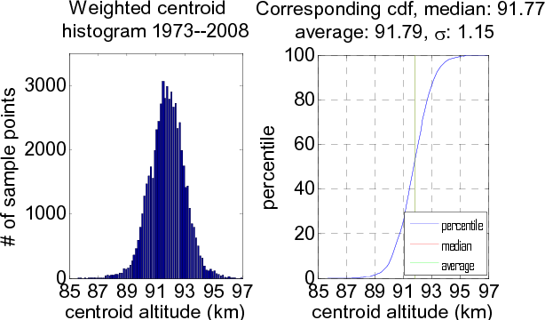
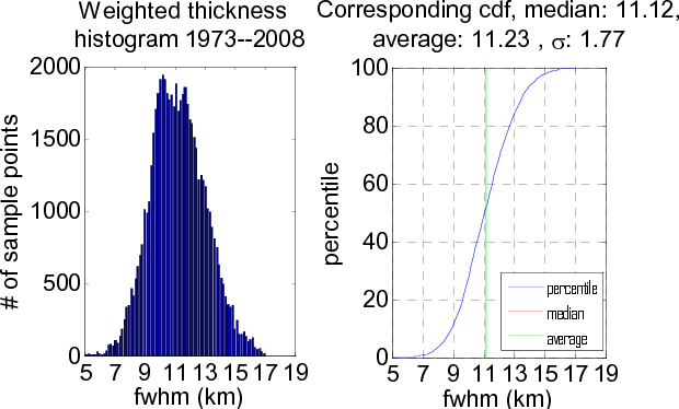
We present in Figs. 2-4, an illustration of the experimental measurement distribution of three parameters of the mesospheric sodium layer: the column abundance, the centroid height, and the sodium layer thickness. We should mention that the data analysis covers mainly three time periods. The number of the sodium vertical distribution profiles measured for each period is 58 625 for the period (1973-2008), 10 780 for the period (1973-1980), and 24 969 for the period (2007-2008).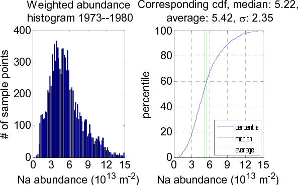
|
Figure 2: Weighted histogram and the cumulative distribution function of column abundance (1973-1980). |
| Open with DEXTER | |
|
Figure 3: Weighted histogram and the cumulative distribution function of the sodium layer centroid height. |
| Open with DEXTER | |
|
Figure 4: Weighted histogram and the cumulative distribution function of sodium layer thickness. Note that the average layer thickness is larger than 10 km, the value used in most published AO simulations. |
| Open with DEXTER | |
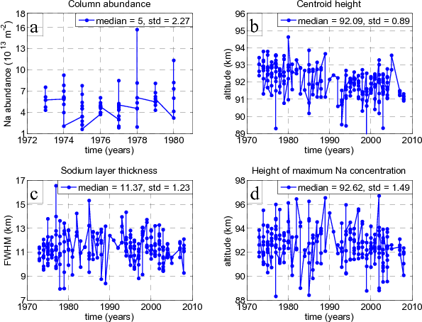
The Fig. 5 presents the
monthly mean values of
the column abundance, centroid height, sodium layer thickness, and
height of the maximum sodium concentration as functions of time.
Accurate measurements of the laser bandwidth were not made
between 1981 and 2006, so data from this period were not included
in the
abundance analysis (see Fig. 5a). The median of the column
abundance is
![]() .
We observe that the column
abundance can reach maximum values of
.
We observe that the column
abundance can reach maximum values of
![]() ,
which
may be caused by sporadic layers.
,
which
may be caused by sporadic layers.
|
Figure 5: Time series of mesospheric sodium layer characteristics. Solid dots represent monthly mean values of each parameter. |
| Open with DEXTER | |
The altitude variation in the sodium layer centroid is a very important phenomenon to consider because in AO closed loop operation it can introduce an offset error in the focus compensation.The mean centroid height is found to vary between 90 km and 94 km and its median is 92.09 km, as seen in Fig. 5b. The sodium layer thickness obtained from its equivalent Gaussian shown in Fig. 5c varies between 8 km and 15 km. Its median is 11.37 km. The height of maximum sodium concentration varies between 90 km and 97 km with a median of 92.62 km. We observe that the height of the maximum sodium concentration is generally larger than the centroid height. Chemistry plays a key role in the equilibrium between the atomic Na and other atoms, ions, and molecules in the upper atmosphere, as described in the following section.
5 Mesospheric sodium layer chemistry
Sodium ions (Na+) and sodium bicarbonate (NaHCO3) are the
main reservoir species above and below the atomic mesospheric sodium
layer, respectively (Fan et al. 2007; Plane et al.
1999). Because of the long residence time (![]() 7 days) of ablated sodium in the region between 80 and 100 km, and the
comparatively short lifetimes of the rate-determining chemical
reactions that convert sodium between atomic Na and these
reservoirs, the chemistry reaches a photochemical steady-state on
the timescale of vertical transport by eddy or molecular diffusion.
The chemical reactions responsible for the conversion of Na to
NaHCO3 occur rapidly and have small temperature dependencies
(Plane 2004, 1998). NaHCO3 is converted
back to Na by the reaction with H. This reaction has a large
activation energy, that is at higher temperatures it becomes much
faster, and the steady-state balance shifts from NaHCO3 to Na
(Cox et al. 2001). It was suggested that the final sink
for sodium on the bottomside of the layer is attachment to aerosol
particles (Hunten et al. 1980).
7 days) of ablated sodium in the region between 80 and 100 km, and the
comparatively short lifetimes of the rate-determining chemical
reactions that convert sodium between atomic Na and these
reservoirs, the chemistry reaches a photochemical steady-state on
the timescale of vertical transport by eddy or molecular diffusion.
The chemical reactions responsible for the conversion of Na to
NaHCO3 occur rapidly and have small temperature dependencies
(Plane 2004, 1998). NaHCO3 is converted
back to Na by the reaction with H. This reaction has a large
activation energy, that is at higher temperatures it becomes much
faster, and the steady-state balance shifts from NaHCO3 to Na
(Cox et al. 2001). It was suggested that the final sink
for sodium on the bottomside of the layer is attachment to aerosol
particles (Hunten et al. 1980).
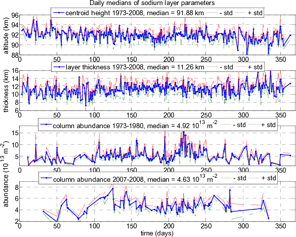
6 Sodium layer parameters variation
We now focus on the variation in the column abundance, the centroid height, and the sodium layer thickness, because these characteristics are very important for the estimation of the laser guide star parameters (sodium photon return, spot size, and spot elongation). The daily medians of the sodium layer parameters calculated over all the experimental period (1973-2008) are presented in Fig. 6.
The sodium thickness
![]() can be defined for
arbitrary sodium profiles,
can be defined for
arbitrary sodium profiles,
![]() ,
as
,
as
The centroid height,
The sodium column density
where
hence
|
Figure 6: Daily medians of sodium layer parameters, where the dashed lines represent the standard deviations for all the data each day. |
| Open with DEXTER | |
The annual median of the centroid height is 91.88 km. The daily
median of this height varies between a maximum of 95 km and a
minimum of 88 km. The layer thickness is calculated from its
equivalent Gaussian. The complexity of the mesospheric sodium layer
structure means that the Gaussian fits are not always very
meaningful, although this information could be very useful for the
determination of the LGS spot elongation. The annual median of the
full width at half maximum (FWHM) of the sodium layer is 11.26 km.
The daily median of this thickness varies between a maximum of 16 km
and a minimum of 8 km. The annual median of the sodium column
abundance is
![]() for the period (1973-1980)
and
for the period (1973-1980)
and
![]() for the period (2007-2008). Its
daily median sometimes reaches a maximum of
for the period (2007-2008). Its
daily median sometimes reaches a maximum of
![]() .
This high value could be explained by the presence of sporadic
layers, although the presence of these layers does not appear to
significantly affect long-term averages (Simonich et al.
2005).
.
This high value could be explained by the presence of sporadic
layers, although the presence of these layers does not appear to
significantly affect long-term averages (Simonich et al.
2005).
Figures 7-9 present a
statistical calculation of the mesospheric sodium layer parameters
for the data of the full observing period, without daily averages.
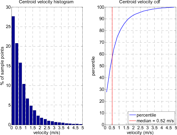
Figure 7 shows that the centroid height is more than 92 km
during 40![]() of the year, with a median value of 91.91 km. The
velocity of vertical displacement of the centroid height is an
important parameter in designing a LGS system. Figure 8
shows that the centroid vertical velocity varies between 0 and 5 m/s, with a median value of 0.52 m/s. During 60
of the year, with a median value of 91.91 km. The
velocity of vertical displacement of the centroid height is an
important parameter in designing a LGS system. Figure 8
shows that the centroid vertical velocity varies between 0 and 5 m/s, with a median value of 0.52 m/s. During 60![]() of the year,
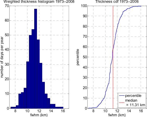
this velocity is less than 0.5 m/s. Figure 9 shows that the
mesospheric sodium layer thickness is between 7 km and 16 km, its
median value being 11.31 km, which is less than its median value
during 60
of the year,
this velocity is less than 0.5 m/s. Figure 9 shows that the
mesospheric sodium layer thickness is between 7 km and 16 km, its
median value being 11.31 km, which is less than its median value
during 60![]() of the year.
of the year.
![\begin{figure}
\par\includegraphics[width=7.5cm,clip]{13281f07.eps}
\end{figure}](/articles/aa/full_html/2010/03/aa13281-09/img36.png)
|
Figure 7: Weighted histogram and the cumulative distribution function of centroid height. |
| Open with DEXTER | |
|
Figure 8: Histogram and the cumulative distribution function of sodium layer centroid velocity, for all the experimental period (1973-2008). |
| Open with DEXTER | |
|
Figure 9: Weighted histogram and the cumulative distribution function of sodium layer thickness. |
| Open with DEXTER | |
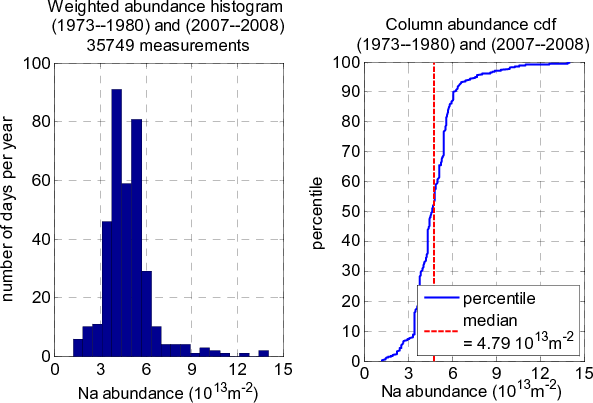
For the column abundance, because of the bandwidth
calibration problem mentioned in Sect. 2, we considered two
periods (1973-1980) and (2007-2008). The close agreement between
the median abundances
![]() for the first
period and
for the first
period and
![]() for the second (see Fig. 6) suggests that the data for the two periods could be
combined to improve the statistics, as shown in Fig. 10.
for the second (see Fig. 6) suggests that the data for the two periods could be
combined to improve the statistics, as shown in Fig. 10.
|
Figure 10: Weighted histogram and the cumulative distribution function of column abundance for the combined periods (1973-1980) and (2007-2008). |
| Open with DEXTER | |
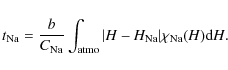
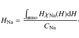
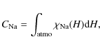
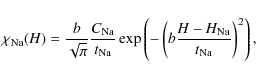
6.1 Estimation of the return flux availability
To estimate the required laser power for the use of adaptive optics,
we calculate the specific return photon flux to the ground. The
expression of this parameter is given by
where
For vertical propagation of the laser beam and assuming
that the centroid height is constant and the coupling efficiency of
light at the sodium wavelength is constant, the return flux can be
assumed to be proportional to the sodium column density. Assuming
that a laser power of 100![]() is needed to produce sufficent sodium
laser-guide-star photon return-flux for a median value of a column
abundance of
is needed to produce sufficent sodium
laser-guide-star photon return-flux for a median value of a column
abundance of
![]() ,
we calculate the number of days
for which the sodium laser-guide-star return is enough for the
adaptive optics (AO) system for low geographic latitude sites as
shown in Fig. 11.
,
we calculate the number of days
for which the sodium laser-guide-star return is enough for the
adaptive optics (AO) system for low geographic latitude sites as
shown in Fig. 11.
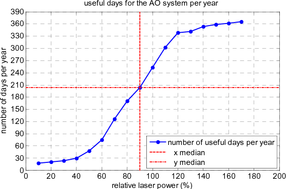
|
Figure 11: Number of useful days per year as function of the Laser power. |
| Open with DEXTER | |
From Fig. 11, we can see that for a laser power
of 100![]() ,
the return flux is assumed to be enough for the AO system during
253 days per year. If we increase the laser power by a
factor of 20
,
the return flux is assumed to be enough for the AO system during
253 days per year. If we increase the laser power by a
factor of 20![]() the number of useful days for the AO system is
around 338 days per year. So the observation with an adaptive optics
system using laser guide stars can practically cover the whole year
for a relative laser power of 120
the number of useful days for the AO system is
around 338 days per year. So the observation with an adaptive optics
system using laser guide stars can practically cover the whole year
for a relative laser power of 120![]() .
.
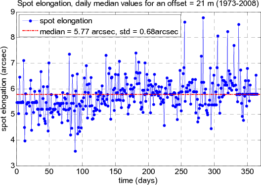
6.2 The LGS spot elongation
The laser-guide-star photon return flux and hence the power
requirement are driven by the spot elongation. It is useful to know
the evolution of this parameter, to optimize the characteristics of
the sodium laser guide star. The angular spot elongation observed
from the ground (see Fig. 12) is given by

where
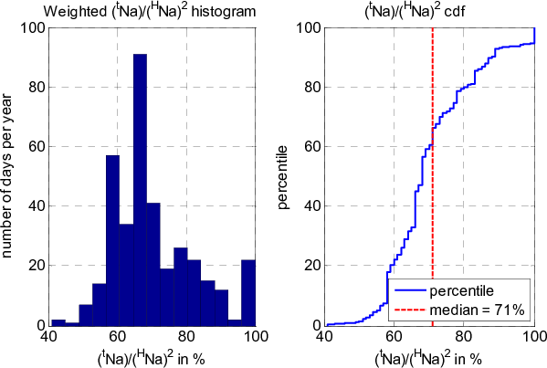
Figure 13 presents a statistical calculation of
the quantity
![]() . For a given
zenith angle
. For a given
zenith angle ![]() and an orthogonal offset
and an orthogonal offset ![]() ,
this
quantity determines the spot elongation. Figure 14 presents
a quantitative estimation of the spot elongation of the sodium laser
guide star in arcsec, for a vertical propagation of the laser beam
and an orthogonal offset
,
this
quantity determines the spot elongation. Figure 14 presents
a quantitative estimation of the spot elongation of the sodium laser
guide star in arcsec, for a vertical propagation of the laser beam
and an orthogonal offset
![]() ,
which corresponds to the
radius of the aperture of the European Extremely Large Telescopes
(E-ELT) planned by ESO (with 42 m aperture diameter).
,
which corresponds to the
radius of the aperture of the European Extremely Large Telescopes
(E-ELT) planned by ESO (with 42 m aperture diameter).
![\begin{figure}
\par\includegraphics[scale=0.4]{13281f12.eps}
\end{figure}](/articles/aa/full_html/2010/03/aa13281-09/img53.png)
|
Figure 12: Schematic drawing of the angular spot elongation as observed from the ground. |
| Open with DEXTER | |
|
Figure 13: Weighted histogram and the cumulative distribution function of the ratio of the layer thickness to the squared centroid height. The latter is a measure of the spot elongation for all the experimental period (1973-2008). |
| Open with DEXTER | |
|
Figure 14: Spot elongation for a vertical propagation of the laser beam and an offset distance of R = 21 m. |
| Open with DEXTER | |
The values of the sodium layer thickness and the centroid
height are the daily medians calculated over all the period
(1973-2008). We can see that the spot elongation for an offset
distance of
![]() ,
is situated between 3 and 9 arcsec, and
that its daily median is 5.77 arcsec with a standard deviation of
0.68 arcsec. If we consider the maximum value of 9 arcsec in Fig. 14, we see from
Fig. 13 that the spot elongation
is less than 6.4 arcsec for more than 60
,
is situated between 3 and 9 arcsec, and
that its daily median is 5.77 arcsec with a standard deviation of
0.68 arcsec. If we consider the maximum value of 9 arcsec in Fig. 14, we see from
Fig. 13 that the spot elongation
is less than 6.4 arcsec for more than 60![]() of the year.
of the year.
7 Nocturnal variation in the sodium layer parameters
Figure 15 shows the hourly median values of the centroid height, the thickness, and the column abundance of the sodium layer. The derivation of a median nocturnal variation is complicated because most of the experimental observations refer to time periods of only a few hours for a given night. As a result of this, the very large night-to-night variations that frequently occur will tend to make the mean nocturnal variation noisier if any simple median is taken. To overcome this problem, we selected nights with enough data to cover many hours of the same night. The hourly median values presented in Fig. 15 are calculated for about 25 000 measurements.![\begin{figure}
\par\includegraphics[width=8cm,clip]{13281f15.eps}
\end{figure}](/articles/aa/full_html/2010/03/aa13281-09/img56.png)
|
Figure 15: Hourly medians of sodium layer parameters, the dashed curves represent the standard deviations for all the data for each hour. Time = 30 h means 0600 local time. |
| Open with DEXTER | |
The column abundance varies between a minimum of
![]() just before midnight and reaches its
maximum value of more than
just before midnight and reaches its
maximum value of more than
![]() at 0500 local
time (29h means five hours after midnight). Its nocturnal median is
at 0500 local
time (29h means five hours after midnight). Its nocturnal median is
![]() .
The centroid height increases during the
night, and reaches a maximum of 91.50 km at 0500 local time. Its
nocturnal median is 91.31 km. The sodium layer thickness starts the
night by decreasing until it reaches a minimum of 10.5 km around
midnight and increases after that to reach a maximum around 12 km at
0500 local time. Its nocturnal median is 11.57 km. It should be
noted that these nocturnal variations are almost certainly tidal in
origin (Batista et al. 1985) and since the phase and
amplitude of atmospheric tides vary during the year (with a mainly
semi-annual oscillation at low latitudes), the temporal variations
shown in Fig. 15 are useful only when considered as annual
averages.
.
The centroid height increases during the
night, and reaches a maximum of 91.50 km at 0500 local time. Its
nocturnal median is 91.31 km. The sodium layer thickness starts the
night by decreasing until it reaches a minimum of 10.5 km around
midnight and increases after that to reach a maximum around 12 km at
0500 local time. Its nocturnal median is 11.57 km. It should be
noted that these nocturnal variations are almost certainly tidal in
origin (Batista et al. 1985) and since the phase and
amplitude of atmospheric tides vary during the year (with a mainly
semi-annual oscillation at low latitudes), the temporal variations
shown in Fig. 15 are useful only when considered as annual
averages.
8 Long term evolution of the sodium layer parameters
8.1 Column abundance
In Fig. 16, we present monthly medians of the sodium column
abundance with circular dots and a solid blue line. The dashed red
and green lines represent respectively ![]() standard deviation from
the monthly median of the column abundance calculated over the
entire experimental period.
standard deviation from
the monthly median of the column abundance calculated over the
entire experimental period.
|
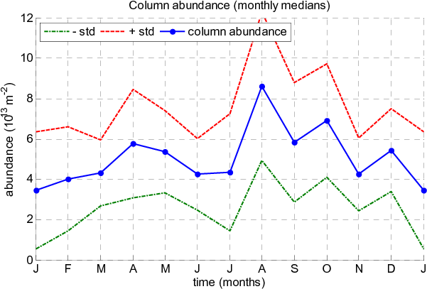
Figure 16: Monthly medians of the mesospheric sodium column abundance, where the standard deviations are calculated for each month throughout the experimental period. |
| Open with DEXTER | |
Figure 16 shows the values of the monthly medians of the column abundance. Each monthly median corresponds to the median of the accumulated data for the same month over the entire experimental measurement period. The sodium column abundance reaches a maximum during the period of (July-August), and a minimum around (February-January). Several authors, such Cox et al. (2001), Xiong et al. (2003), and Drummond et al. (2007) noted that the time evolution of the mesospheric sodium column abundance has a characteristic period of one year. It is tempting to suggest that the maximum of the sodium column abundance could be explained by the increase in the meteoric input during this period, which is rich in terms of meteor showers. The most visible meteor shower called the Perseids occurs each year during the period (July 17 to August 24), and peaks in mid-August at over 1 meteor a minute. Another strong meteor shower is observed during this period called south Delta Aquarids (July 12 to August 19). However, it has long been known that the sodium layer variation is seasonal, rather than annual, with a winter abundance maximum in both the northern and southern hemispheres. This winter maximum appears to be the effect of the seasonal temperature variation in the reactions that recycle sodium compounds back to free sodium (Plane et al. 1999).
8.2 Centroid height
To determine in more detail the centroid height evolution during
long-term observations we calculated its monthly medians. Each
median was calculated for a given month of the year on the basis of
the entire period of the data measurements. In Fig. 17,
these values are represented by circular dots and a solid blue line.
The dashed red and green lines represent respectively ![]() the
standard deviation of the monthly medians of the centroid height
calculated over the entire experimental period.
the
standard deviation of the monthly medians of the centroid height
calculated over the entire experimental period.
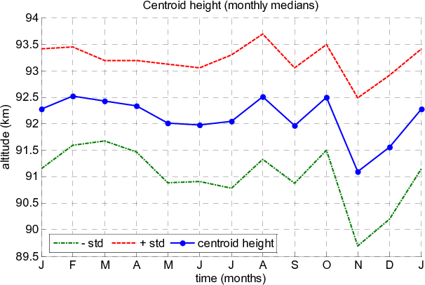
|
Figure 17: Monthly medians of the mesospheric sodium layer centroid height, the standard deviations are calculated for each month throughout the experimental period. |
| Open with DEXTER | |
The sharp minimum in November appears to represent a true geophysical effect which is believed to be tidal in origin (Clemesha et al. 2005). Apart from this November minimum, the centroid height appears to exhibit a predominantly semi-annual variation, in agreement with Xiong et al. (2003). A semi-annual oscillation is likely to be associated with tides and gravity waves (Clemesha et al. 2005, 2009). It is possible that the August maximum in centroid height is related to the strong meteor showers that occur in that month.
9 Conclusion
This paper has analyzed a large sample of mesospheric sodium data, collected in the southern hemisphere over 35 years, at latitudes similar to that of the ESO Paranal observatory in Chile, to derive statistically meaningful parameters relevant for adaptive optics with laser guide stars at 589nm. This analysis has provided much needed mesospheric sodium parameter statistics, which are meaningful because they were obtained for more than a few samples.
The knowledge of the statistics of the mesospheric sodium layer parameters allows those developing adaptive optics with sodium LGSs to better simulate and design the LGS-AO systems more accurately, as well as to dimension the laser system to secure the availability for observations. This knowledge is in particularly important for the design e.g, of the second generation ESO VLT and the new E-ELT LGS-AO systems.
Assuming that for a given laser power and a sodium column
abundance of
![]() ,
the photon return flux is
sufficient for the AO system, the telescope can observe with the AO
system using sodium LGSs, over more than 250 days per year. An
increasing of the laser power by 20
,
the photon return flux is
sufficient for the AO system, the telescope can observe with the AO
system using sodium LGSs, over more than 250 days per year. An
increasing of the laser power by 20![]() allows us to cover the
entire year.
allows us to cover the
entire year.
The specific photon return flux reaches its maximum values during July-August in the southern hemisphere. This effect can be explained by the increase in meteoric ablation during this period, which is rich in terms of meteoric showers, and/or by the mesospheric sodium chemistry, which is related to the winter maximum in mesopause region temperature.
The median value of the sodium LGS spot elongation for an
offset distance of
![]() ,
is 5.77 arcsec. The average
values of the sodium layer parameters calculated over all the
experimental period (1973-2008) are 92.09 km for the centroid
height, 11.37 km for the layer thickness, and
,
is 5.77 arcsec. The average
values of the sodium layer parameters calculated over all the
experimental period (1973-2008) are 92.09 km for the centroid
height, 11.37 km for the layer thickness, and
![]() for the column abundance. The experimental observation times are
distributed randomly, and 58 625 sodium profiles data have been
taken into account, so the statistical accuracies of our
measurements should be high.
for the column abundance. The experimental observation times are
distributed randomly, and 58 625 sodium profiles data have been
taken into account, so the statistical accuracies of our
measurements should be high.
This work was possible thanks to the R
D activities of the Laser Systems Department, funded by the ESO Technology Division under Job994. For the Lidar measurements, financial support has been received from the Fundação de Amparo à Pesquisa do Estado de São Paulo (FAPESP) and the Conselho Nacional de Desenvolvimento Cientifico e Tecnológico (CNPq).
References
- Batista, P. P., Clemesha, B. R., Simonich, D. M., & Kirchhoff, V. W. J. H. 1985, J. Geophys. Res., 90, 3881 [NASA ADS] [CrossRef] [Google Scholar]
- Clemesha, B. R., Kirchhoff, V. W. J. H., & Simonich, D. M. 1979, Planet. Space Sci., 27, 909 [NASA ADS] [CrossRef] [Google Scholar]
- Clemesha, B. R., Simonich, D. M., & Batista, P. P. 1992, Geophys. Res. Lett., 19, 457 [NASA ADS] [CrossRef] [Google Scholar]
- Clemesha, B. R., Batista, P. P., & Simonich, D. M. 2001, Adv. Space Res., 27, 1679 [NASA ADS] [CrossRef] [Google Scholar]
- Clemesha, B. R., Simonich, D. M., Vondrak, T.,& Plane, J. M. C. 2004, J. Geophys. Res., 109, D05302 [CrossRef] [Google Scholar]
- Clemesha, B. R., Simonich, D. M., Batista, P. P., & Takahashi, H. 2005, Adv. Space Res., 35(11), 1951 [NASA ADS] [CrossRef] [Google Scholar]
- Clemesha, B. R., Batista, P. P, Costa, R. B. D., & Schuch, N. 2009, Annales Geophysicae, 27, 1059 [NASA ADS] [CrossRef] [Google Scholar]
- Cox, R. M., Self, D. E., & Plane, J. M. C. 2001, J. Geophys. Res., 106, 1733 [NASA ADS] [CrossRef] [Google Scholar]
- Drummond, J., Novotny, S., Denman, C., et al. 2007, The Sodium LGS Brightness Model over the SOR, AMOS Technical Conference [Google Scholar]
- Fan, Z. Y., Plane, J. M. C., Gumbel, J., Stegman, J., & Llewellyn, E. J. 2007, Atmos. Chem. Phys., 7, 4107 [Google Scholar]
- Gardner, C. S., Senft, D. C., & Kwon, K. H. 1988, Nature, 332, 142 [NASA ADS] [CrossRef] [Google Scholar]
- Gardner, C. S., Plane, J. M. C., Pan, W., et al. 2005, J. Geophys. Res., 110, D10302 [NASA ADS] [CrossRef] [Google Scholar]
- Hunten, D. M., Turco, R. P., & Toon, O. B. 1980, J. Atmos. Terr., 37, 1342 [NASA ADS] [Google Scholar]
- Kirchhoff, V. W. J. H., & Clemesha, B. R. 1983, J. Geophys. Res., 88, 442 [NASA ADS] [CrossRef] [Google Scholar]
- Megie, G., & Blamont, J. E. 1977, Planet. Space Sci., 25, 1093 [NASA ADS] [CrossRef] [Google Scholar]
- Moussaoui, N., Holzlöhner, R., Hackenberg, W., & Bonaccini Calia, D. 2008, Proc. SPIE, 7015, 70152W1-10 [CrossRef] [Google Scholar]
- Moussaoui, N., Holzlöhner, R., Hackenberg, W., & Bonaccini Calia, D. 2009, A&A, 501, 793 [NASA ADS] [CrossRef] [EDP Sciences] [Google Scholar]
- Plane, J. M. C. 2003, Chem. Rev., 103, 4963 [Google Scholar]
- Plane, J. M. C. 2004, Atmos. Chem. Phys., 4, 627 [NASA ADS] [CrossRef] [Google Scholar]
- Plane, J. M. C., Cox, R. M., Qian, J., et al. 1998, J. Geophys. Res., 103, 6381 [NASA ADS] [CrossRef] [Google Scholar]
- Plane, J. M. C., Gardner, C. S., Yu, J. R., et al. 1999, J. Geophys. Res., 104, 3773 [NASA ADS] [CrossRef] [Google Scholar]
- She, C. Y., Chen, S. S., Hu, Z. L., et al. 2000, Geophys. Res. Lett., 27, 3289 [NASA ADS] [CrossRef] [Google Scholar]
- Simonich, D. M., Clemesha, B. R., & Kirchhoff, V. W. J. H. 1978, Trans. Am. Geophys. Union, 59, 342 [Google Scholar]
- Simonich, D. M., Clemesha, B. R., & Kirchhoff, V. W. J. H. 1979, J. Geophys. Res., 84, 1543 [NASA ADS] [CrossRef] [Google Scholar]
- Simonich, D. M., Clemesha, B. R., & Batista, P. P. 2005, Adv. Space Sci., 35(11), 1976 [NASA ADS] [CrossRef] [Google Scholar]
- Tilgner, C., & von Zahn, U. 1988, J. Geophys. Res., 93, 8439 [NASA ADS] [CrossRef] [Google Scholar]
- Xiong, H. U., Gardner, C. S., & Liu, A. Z. 2003, Chin. J. Geophys., 46, 3, 432 [Google Scholar]
- von Zahn, U., Hansen, G., Kurzawa, H., et al. 1988, Nature, 331, 594 [NASA ADS] [CrossRef] [Google Scholar]
All Figures
|
|
Figure 1: Simplified plan view: optical layout for INPE Lidar. |
| Open with DEXTER | |
| In the text | |
|
|
Figure 2: Weighted histogram and the cumulative distribution function of column abundance (1973-1980). |
| Open with DEXTER | |
| In the text | |
|
|
Figure 3: Weighted histogram and the cumulative distribution function of the sodium layer centroid height. |
| Open with DEXTER | |
| In the text | |
|
|
Figure 4: Weighted histogram and the cumulative distribution function of sodium layer thickness. Note that the average layer thickness is larger than 10 km, the value used in most published AO simulations. |
| Open with DEXTER | |
| In the text | |
|
|
Figure 5: Time series of mesospheric sodium layer characteristics. Solid dots represent monthly mean values of each parameter. |
| Open with DEXTER | |
| In the text | |
|
|
Figure 6: Daily medians of sodium layer parameters, where the dashed lines represent the standard deviations for all the data each day. |
| Open with DEXTER | |
| In the text | |
|
|
Figure 7: Weighted histogram and the cumulative distribution function of centroid height. |
| Open with DEXTER | |
| In the text | |
|
|
Figure 8: Histogram and the cumulative distribution function of sodium layer centroid velocity, for all the experimental period (1973-2008). |
| Open with DEXTER | |
| In the text | |
|
|
Figure 9: Weighted histogram and the cumulative distribution function of sodium layer thickness. |
| Open with DEXTER | |
| In the text | |
|
|
Figure 10: Weighted histogram and the cumulative distribution function of column abundance for the combined periods (1973-1980) and (2007-2008). |
| Open with DEXTER | |
| In the text | |
|
|
Figure 11: Number of useful days per year as function of the Laser power. |
| Open with DEXTER | |
| In the text | |
|
|
Figure 12: Schematic drawing of the angular spot elongation as observed from the ground. |
| Open with DEXTER | |
| In the text | |
|
|
Figure 13: Weighted histogram and the cumulative distribution function of the ratio of the layer thickness to the squared centroid height. The latter is a measure of the spot elongation for all the experimental period (1973-2008). |
| Open with DEXTER | |
| In the text | |
|
|
Figure 14: Spot elongation for a vertical propagation of the laser beam and an offset distance of R = 21 m. |
| Open with DEXTER | |
| In the text | |
|
|
Figure 15: Hourly medians of sodium layer parameters, the dashed curves represent the standard deviations for all the data for each hour. Time = 30 h means 0600 local time. |
| Open with DEXTER | |
| In the text | |
|
|
Figure 16: Monthly medians of the mesospheric sodium column abundance, where the standard deviations are calculated for each month throughout the experimental period. |
| Open with DEXTER | |
| In the text | |
|
|
Figure 17: Monthly medians of the mesospheric sodium layer centroid height, the standard deviations are calculated for each month throughout the experimental period. |
| Open with DEXTER | |
| In the text | |
Copyright ESO 2010
Current usage metrics show cumulative count of Article Views (full-text article views including HTML views, PDF and ePub downloads, according to the available data) and Abstracts Views on Vision4Press platform.
Data correspond to usage on the plateform after 2015. The current usage metrics is available 48-96 hours after online publication and is updated daily on week days.
Initial download of the metrics may take a while.