| Issue |
A&A
Volume 510, February 2010
|
|
|---|---|---|
| Article Number | A83 | |
| Number of page(s) | 25 | |
| Section | Cosmology (including clusters of galaxies) | |
| DOI | https://doi.org/10.1051/0004-6361/200913156 | |
| Published online | 16 February 2010 | |
Cool core remnants in galaxy clusters![[*]](/icons/foot_motif.png)
M. Rossetti - S. Molendi
Istituto di Astrofisica Spaziale e Fisica Cosmica, INAF, via Bassini 15, 20133 Milano, Italy
Received 20 August 2009 / Accepted 20 October 2009
Abstract
Context. X ray clusters are conventionally divided into two
classes: ``cool core'' (CC) and ``non-cool core'' (NCC) objects, on the
basis of the observational properties of their central regions. Recent
results have shown that the cluster population is bimodal.
Aims. We want to understand whether the observed distribution of
clusters is due to a primordial division into two distinct classes or
rather to differences in the way these systems evolve across cosmic
time.
Methods. We systematically search the ICM of NCC clusters in a
subsample of the B55 flux limited sample of clusters for regions
which have some characteristics typical of cool cores, namely low
entropy gas and high metal abundance.
Results. We find that most NCC clusters in our sample host
regions reminiscent of CC, i.e. characterized by relative low
entropy gas (albeit not as low as in CC systems) and a metal
abundance excess. We have dubbed these structures ``cool core
remnants'', since we interpret them as the remains of a cool core after
a heating event (AGN giant outbursts in a few cases and more commonly
mergers). We infer that most NCC clusters have undergone a cool
core phase during their life. The fact that most cool core remnants are
found in dynamically active objects provides strong support to
scenarios where cluster core properties are not fixed ``ab initio'' but
evolve across cosmic time.
Key words: galaxies: clusters: general - X-rays: galaxies: clusters
1 Introduction
Galaxy clusters are often divided by X-ray astronomers into two
classes: ``cool core''(CC) and ``non-cool core'' (NCC) clusters. The
former are characterized by a set of properties: a prominent surface
brightness peak, usually roughly coincident with the center of the
large scale X-ray isophotes and with the position of the brightest
central galaxy (BCG), associated with a decrease of the temperature
profile in the inner regions and a positive gradient of the metal
abundance profile. In the central regions of these clusters, the
cooling time is significantly smaller than the Hubble time, but the
radiative losses are balanced by some form of heating, which in the
currently prevailing scenario is attributed to the central AGN, which
prevents the gas from cooling indefinitely and flowing inward.
NCC clusters are characterized by the lack of these observational
features. Several indicators based on these observational
characteristics have been proposed to classify clusters into these
categories: e.g. temperature drop (Sanderson et al. 2006,2009b), cooling time (Bauer et al. 2005), a composition of these two criteria (Dunn & Fabian 2008; Dunn et al. 2005), the slope of the gas density profile at a given radius (Vikhlinin et al. 2007) and core entropy (Cavagnolo et al. 2009). In a recent paper (Leccardi et al. 2010, hereafter Paper I), we suggested a robust indicator to classify clusters (see also Sect. 3),
based on pseudo-entropy gradients. The classification based on this
indicator improves the traditional classification scheme based on the
temperature drop and is essentially equivalent to classifications based
on the cooling time. Increasing attention has been devoted to the
statistics of CC, both in the local Universe and at higher redshifts.
While the precise results depend strongly on the indicator used to
classify clusters, the fraction of CC is considered to be about ![]() of the clusters population. There are some indication that the cluster population is bimodal (Cavagnolo et al. 2009), but there are also some intermediate objects which are not easily classified (Paper I).
of the clusters population. There are some indication that the cluster population is bimodal (Cavagnolo et al. 2009), but there are also some intermediate objects which are not easily classified (Paper I).
One of the open questions in the study of galaxy clusters concerns the origin of this distribution. The original model which prevailed for a long time assumed that the CC state was a sort of ``natural state'' for the clusters, and the observational features were explained within the context of the old ``cooling flow'' model: radiation losses cause the gas in the centers of these clusters to cool and to flow inward. Clusters were supposed to live in this state until disturbed by a ``merger''. Indeed, mergers are very energetic events that can shock-heat (Burns et al. 1997) and mix the ICM (Ritchie & Thomas 2002; Gómez et al. 2002): through these processes they were supposed to efficiently destroy cooling flows. After the mergers, clusters were supposed to relax and go back to the cooling flow state in a sort of cyclical evolution. With the fall of the ``cooling flow'' brought about by the XMM-Newton and Chandra observations (e.g. Peterson et al. 2001; Molendi & Pizzolato 2001), doubts were cast also on the interpretation of mergers as the dominant mechanism which could transform CC clusters into NCC. More generally speaking, the question arose whether the observed distribution of clusters was due to a primordial division into the two classes or rather to evolutionary differences during the history of the clusters.
McCarthy et al. (2008,2004)
noticed the absence of systems that resemble observed NCC clusters
in cosmological simulations, suggesting that mergers could not be the
origin of the cluster distribution. They proposed that early episodes
of non-gravitational pre-heating may explain the dichotomy; they
envisage a scenario in which NCC clusters have been pre-heated to
levels greater than
![]() and did not have enough time to develop a cool core, while
CC clusters have been pre-heated to lower levels and need an
additional source of present-day heating to offset cooling. With this
model, McCarthy et al. (2008) explained observed entropy and gas density Chandra profiles for CC and ROSAT gas density profiles for NCC. O'Hara et al. (2006)
supported the primordial model, showing that the scatter in scaling
relations is larger for CC clusters than for NCC, suggesting that
CC are not more relaxed than NCC systems. Moreover the two-body
idealized simulations by Poole et al. (2008) showed that mergers cannot produce extended ``warm'' cores and cannot destroy metal abundance gradients.
and did not have enough time to develop a cool core, while
CC clusters have been pre-heated to lower levels and need an
additional source of present-day heating to offset cooling. With this
model, McCarthy et al. (2008) explained observed entropy and gas density Chandra profiles for CC and ROSAT gas density profiles for NCC. O'Hara et al. (2006)
supported the primordial model, showing that the scatter in scaling
relations is larger for CC clusters than for NCC, suggesting that
CC are not more relaxed than NCC systems. Moreover the two-body
idealized simulations by Poole et al. (2008) showed that mergers cannot produce extended ``warm'' cores and cannot destroy metal abundance gradients.
However, the evolutionary ``merger'' scenario has been continuously supported by observations. For instance, Sanderson et al. (2006) compared temperature and cooling time profiles of a sample of clusters observed by Chandra with indicators of merger activity and suggested that mergers may be the primary factor in preventing the formation of CCs. More recently, Sanderson et al. (2009a) have shown in a large sample of objects that the X-ray/BCG projected offset correlates with the gas density profile, which can be considered an indicator of the CC state. If the X-ray/BCG offset ``measures'' the dynamical state of the cluster, this result implies that the cool core strengths diminishes in more dynamically disturbed clusters. Another indicator of dynamical activity is the presence of extended radio halos on Mpc scales, whose origin is likely related to turbulent acceleration driven by mergers (Ferrari et al. 2008, for a recent review). None of the clusters which are found to host a radio halo (on Mpc scales) in a complete survey (Brunetti et al. 2009; Venturi et al. 2008) can be classified as a CC object. These relations are indeed expected if mergers can efficiently destroy cool cores.
An interesting model has been proposed by Motl et al. (2004), who suggested a double role for mergers in the cluster formation process: while they can shock-heat the ICM, they also efficiently mix the ICM and participate in the formation of CCs by providing cool gas. By analyzing simulated temperature and surface brightness maps, they find that observational signatures of a cool core may disappear after mergers, but that cool gas remains in the systems at all time. Indeed, mergers are complicated phenomena during which the ICM of the interacting objects is mixed. Also the simulations by Ascasibar & Markevitch (2006) on the formation of cold fronts showed that an interacting subcluster may donate its cool gas to the main cluster and that, during the merging processes, many hydrodynamic effects contribute to the mixing of the gas.
Recently, we found an unexpected and interesting result from the analysis of the metalicity profiles in a large sample of clusters (Paper I): some clusters that cannot be classified as CC show a metal abundance excess at their center, without a significant temperature decline or an X-ray brightness excess. We suggested that at least some NCC clusters have spent part of their lives as CC objects and that consequently a complete primordial separation of the two classes of objects cannot be the case.
However, further analysis is needed on this result to use it to gain insight on the origin of the distribution of CC-NCC objects. We would like to characterize these regions better and to know if and to what extent they are common in the population of NCC objects. The results in Paper I as well as those described above comparing observations and simulation, are based on ``uni-dimensional'' properties (entropy and metal abundance profiles). Indeed, global properties and unidimensional profiles are easy to derive and it is possible to compare them quantitatively, but they inevitably result in a loss of information. Many thermodynamic maps are now available in the literature, which show that spherical symmetry is not generally fulfilled in clusters, and which reveal the presence of regions with ``anomalous'' characteristics outside of the cores (e.g. Rossetti et al. 2007; Sun et al. 2002, and many others).
In this paper, we present a systematic two-dimensional analysis of a sample of 35 clusters observed with XMM-Newton,
to look for and characterize regions with a significant metal excess in
NCC clusters, like the ones found in Paper I. The outline of
the paper is as follows: in Sect. 2 we describe the
sample and the data analysis, in Sect. 3 we discuss the
classification schemes and we define ``CC remnants'' in
Sect. 4. We interpret our results in Sect. 5, and we
summarize our findings in Sect. 6. Quoted confidence intervals
are 68% for one interesting parameter unless otherwise stated. All
results are given assuming a ![]() CDM cosmology with
CDM cosmology with
![]() ,
,
![]() ,
and H0 = 70 km s-1 Mpc-1.
,
and H0 = 70 km s-1 Mpc-1.
2 Data analysis
2.1 The sample
The starting point of the sample of galaxy clusters described in this paper is the ``B55'' X-ray flux limited sample (Edge et al. 1990).
In order to have a significant coverage of the cluster within
EPIC field of view, we have eliminated the nearest clusters and
considered only those with redshift z > 0.03. Then we analyzed all public XMM-Newton observations, including mosaics and multiple observations, as described in Sect. 2.2. We discarded observations where, after soft proton cleaning, the effective exposure time (
![]() )
is lower than 25 ks, except in the case of mosaics where observations with
)
is lower than 25 ks, except in the case of mosaics where observations with
![]() ks have been used for images but not for spectral analysis.
ks have been used for images but not for spectral analysis.
The list of the clusters which remained after our selection criteria is given in Table 1. A644, A2244 have not been observed by XMM-Newton, while all the observations of A3391, A1736, A2142, A2063 and A1651 are badly contaminated by soft protons (
![]() ks)
and have been discarded. The cluster Cygnus A has been discarded
in a second phase of the analysis because of the presence of the radio
galaxy QSO B1957+405, featuring large hotspots well detected
in X-rays, which cannot be easily subtracted from the core spectrum.
ks)
and have been discarded. The cluster Cygnus A has been discarded
in a second phase of the analysis because of the presence of the radio
galaxy QSO B1957+405, featuring large hotspots well detected
in X-rays, which cannot be easily subtracted from the core spectrum.
2.2 General data reduction
We retrieve Observation Data Files (ODF) from the XMM-Newton
archive and process them with SAS software version 7.0. The event
files produced by this standard analysis technique are then cleaned to
remove soft proton flares with a double filtering process.
As a first step, we produce the light curve in a hard energy
band (10-12 keV) and remove all time periods with count rates
exceeding a fixed threshold
![]() for the MOS detectors and
for the MOS detectors and
![]() for the pn. This procedure allows the removal of most flares, but
softer flares may survive. In the second step, we apply a
for the pn. This procedure allows the removal of most flares, but
softer flares may survive. In the second step, we apply a ![]() clipping
technique to the histogram obtained from the light curve in the
2-5 keV energy range. For each observation, we have calculated the
``in over out ratio'',
clipping
technique to the histogram obtained from the light curve in the
2-5 keV energy range. For each observation, we have calculated the
``in over out ratio'',
![]() (De Luca & Molendi 2004),
to identify observations badly contaminated by a quiescent soft
proton component. As outlined in Paper I, the ratio has been
calculated in an external annulus at E>9 keV to reduce
the contribution of the cluster emission which fills all the FOV,
especially for the nearest objects. We have discarded only one
observation (and therefore the cluster A2065) where the
(De Luca & Molendi 2004),
to identify observations badly contaminated by a quiescent soft
proton component. As outlined in Paper I, the ratio has been
calculated in an external annulus at E>9 keV to reduce
the contribution of the cluster emission which fills all the FOV,
especially for the nearest objects. We have discarded only one
observation (and therefore the cluster A2065) where the
![]() of
the two MOS is larger than 2.0. After soft proton cleaning we
filter the event files according to pattern and flag criteria, and we
remove by sight brightest point sources.
of
the two MOS is larger than 2.0. After soft proton cleaning we
filter the event files according to pattern and flag criteria, and we
remove by sight brightest point sources.
Since we are mainly interested in characterizing the
thermodynamic properties of the ICM in the central and brightest
regions of the clusters of our sample, advanced procedures to treat the
background (Leccardi & Molendi 2008b) are not strictly necessary. This is also the reason why we could discard only badly contaminated observations with
![]() .
As background event files, we merge nine ``blank sky'' field
observations, as is commonly done, and we extract images and
spectra for the background in the same way than for the source
observations. We calculate a normalization factor Q
for each cluster observation to take into account possible temporal
variations of the instrumental background. The normalization factor is
the count rate ratio between source and background observations in an
external ring (
.
As background event files, we merge nine ``blank sky'' field
observations, as is commonly done, and we extract images and
spectra for the background in the same way than for the source
observations. We calculate a normalization factor Q
for each cluster observation to take into account possible temporal
variations of the instrumental background. The normalization factor is
the count rate ratio between source and background observations in an
external ring (
![]() )
beyond 9 keV. Background images and spectra are scaled by Q before the subtraction from source images and spectra.
)
beyond 9 keV. Background images and spectra are scaled by Q before the subtraction from source images and spectra.
2.3 Two-dimensional analysis
For all the clusters in our sample we prepared two dimensional maps of the main thermodynamic quantities, starting from EPIC images. To do this we have used a modified version of the adaptive binning + broad band fitting technique described in Rossetti et al. (2007), where we have substituted the Cappellari & Copin (2003) adaptive binning algorithm with the weighted Voronoi tessellation by Diehl & Statler (2006) (Rossetti 2006).
Especially in clusters undergoing major mergers, where there is no spherical symmetry, maps are a fundamental tool to select interesting regions for a proper spectral analysis, which is necessary to complement the thermodynamical information with the chemical information. Indeed, a ``blind'' spectral analysis in concentric annuli would not allow to detect interesting features in some of our clusters.
2.4 One-dimensional analysis
2.4.1 Profiles
As a first step, we have performed spectral extraction and analysis in concentric annuli. As discussed in Sect. 2.3, the main drawback of this technique is that the assumption of spherical symmetry is not always fulfilled in our clusters, and in some cases even the choice of the center can have a strong impact on the observed properties. Therefore we have used the thermodynamic maps (Sect. 2.3) to identify those clusters where the deviations from the spherical symmetry are larger, and we have decided not to perform radial analysis in four well known merging objects: A3667 (Briel et al. 2004), A2256 (Sun et al. 2002), A754 (Henry et al. 2004) and A3266 (Finoguenov et al. 2006).
For the remaining clusters of the sample, where we do not observe large displacements between the surface brightness peak and the entropy minimum, we select as center of symmetry the surface brightness peak, even if the large scale isophotes have another center. This allows a better description of the ICM properties in the more central regions of the clusters.
We extract spectra from annular regions around the selected center. For each instrument (MOS1, MOS2 and pn) and each region we extract source and background spectra, and we generate an effective area (ARF) file. Then we associate a redistribution matrix file to the spectrum, appropriated for the instrument and, in the pn case, for the position of the selected region in the detector.
We perform spectral fitting, using the XSPEC v11.3 package, separately
for each spectrum in the energy range 0.5-10 keV. We use an
absorbed mekal model (WABS*MEKAL), where the ![]() is fixed to the input galactic value
is fixed to the input galactic value![]() and the redshift is allowed to vary in a small range (width
and the redshift is allowed to vary in a small range (width
![]() )
around the nominal value. Temperature, metal abundance
)
around the nominal value. Temperature, metal abundance![]() and normalization are the free parameters of the fit (following the prescription in Leccardi & Molendi 2008a,
even negative values are allowed for the metal abundance). Best fit
results obtained from the three instruments and from multiple
observations of the same region are then averaged together with a
weighted mean. This enables us to produce the projected
temperature, metal abundance and surface brightness profiles for each
cluster.
and normalization are the free parameters of the fit (following the prescription in Leccardi & Molendi 2008a,
even negative values are allowed for the metal abundance). Best fit
results obtained from the three instruments and from multiple
observations of the same region are then averaged together with a
weighted mean. This enables us to produce the projected
temperature, metal abundance and surface brightness profiles for each
cluster.
Finally, we perform a deprojection of the profiles, following the technique described in Ettori et al. (2002), to derive the three-dimensional density and temperature profiles. Combining them, we obtain entropy and cooling time profiles.
Table 2: Properties of the clusters in the sample: the first 14 entries are LEC clusters, while the remaining are non-LEC.
2.4.2 IN and OUT regions
In order to classify clusters according to the scheme described in
Paper I, we extracted spectra in an IN region and an
OUT reference region, whose radii are defined as a fixed fraction
of R180 (
r<0.05 R180 and
0.05 R180<r<0.2 R180, respectively). R180 has been calculated as
|
(1) |
where
As discussed in Sect. 2.3, the choice of the center has been performed starting from the thermodynamic maps. More specifically, we have selected as a center the position of the minimum in the pseudo-entropy map. In most cases, the position of the entropy minimum coincides with the surface brightness peak, while in other clusters there is a significant displacement, but usually smaller then the radius of the IN regions, with the exception of A3667. Moreover the choice of the position of the entropy minimum as a center instead of the surface brightness peak does not significantly alter the value of the pseudo entropy ratio, except for the case of A3667. This is a well studied merging cluster (Vikhlinin et al. 2001; Briel et al. 2004): the low-entropy gas is concentrated at the position of a prominent cold front about 500 kpc SE from the surface brightness peak (see the figure in Appendix B).
3 Classification schemes
![\begin{figure}
\par\includegraphics[width=8cm,clip]{13156f1.eps}
\end{figure}](/articles/aa/full_html/2010/02/aa13156-09/img97.png)
|
Figure 1:
Comparison of temperature and emission measure ratios for the clusters
in our sample. The solid line represents the threshold used to divide
clusters between low entropy clusters and non-low entropy clusters,
corresponding to
|
| Open with DEXTER | |
As in Paper I we plot the temperature ratios (
![]() )
versus the emission measure ratios (
)
versus the emission measure ratios (
![]() )
for the clusters of our sample (Fig. 1), and we use pseudo-entropy ratios to divide clusters into two classes (Table 2). We recall here the definition of the pseudo-entropy ratio
)
for the clusters of our sample (Fig. 1), and we use pseudo-entropy ratios to divide clusters into two classes (Table 2). We recall here the definition of the pseudo-entropy ratio![]() :
:
The pseudo-entropy ratio is well correlated with the entropy ratio (see Appendix A), and therefore it is a useful and easy-to-calculate indicator of the variation of the physical three-dimensional entropy in the cores of galaxy clusters.
As in Paper I, we compare our pseudo-entropy classification with two alternative classification schemes, based on the core properties (Col. 6 in Table 2) and on the dynamical state (Col. 7 in Table 2). More specifically, in Col. 6 we divide clusters into three classes: cool core (CC), intermediate systems (INT) and non-cool core (NCC), where CC feature a prominent surface brightness peak and a temperature gradient, NCC possess neither of these properties, while INT show only one of these observational features. In Col. 7 we divide clusters into two classes: major mergers (MRG) and clusters showing no evidence of a major merger (NOM). We consider as evidence of a major merger the presence of cluster-wide diffuse radio emission, multi peaked velocity distribution of galaxies and significant irregularities on the surface brightness and temperature maps. The lack of these properties is not sufficient to state that an object is relaxed, this is why we prefer to consider these objects as ``not observed mergers''. We refer to Paper I for more details on the classification schemes and also for the necessary references.
For the purposes of this paper, we are interested in separating
clusters with a low entropy core (LEC) from the rest, this is why we
have defined only one threshold to divide LEC from
non-LEC objects. With our selected threshold (
![]() )
we can state that all LEC clusters are known to be CC and do not
show any evidence of a merger (except A85, probably undergoing a
merger in an early stage, which has not affected the observational
properties of the core, see Paper I). Non-LEC clusters are
almost all non-cool core systems, and many of them show significant
indications of a major merger. As already discussed, the fact that
some of them do not show significant merger features does not mean that
they are relaxed.
)
we can state that all LEC clusters are known to be CC and do not
show any evidence of a merger (except A85, probably undergoing a
merger in an early stage, which has not affected the observational
properties of the core, see Paper I). Non-LEC clusters are
almost all non-cool core systems, and many of them show significant
indications of a major merger. As already discussed, the fact that
some of them do not show significant merger features does not mean that
they are relaxed.
4 Cool core remnants
The central regions of LEC clusters in our sample are characterized by
low-entropy (by definition), often accompanied by a temperature
decrease and a surface brightness excess. These regions are also
characterized by a high metal abundance: the mean iron abundance in the
cores of LEC clusters is significantly larger than the typical
value of outer regions of galaxy clusters
![]() (Leccardi & Molendi 2008a), even if with a
(Leccardi & Molendi 2008a), even if with a
![]() scatter (De Grandi & Molendi 2009).
It has been shown that the excess abundance can be entirely
produced by the BCG galaxy that is invariably found in these
systems (De Grandi et al. 2004).
At present, we are not aware of any galaxy cluster with central
regions characterized by a low entropy gas without a metal abundance
excess. A close relation between entropy and metal abundance must
consequently exist and also generally speaking between the
thermodynamics and the chemical properties of the ICM. An example
of this relation can be seen in Fig. 2,
where we plot the metal abundance radial profile as a function of the
pseudo-entropy ratio for each LEC cluster. The pseudo entropy
ratio is similar to the one defined in Eq. (2), with the one difference that the temperature and emission measure of a given annulus replace
scatter (De Grandi & Molendi 2009).
It has been shown that the excess abundance can be entirely
produced by the BCG galaxy that is invariably found in these
systems (De Grandi et al. 2004).
At present, we are not aware of any galaxy cluster with central
regions characterized by a low entropy gas without a metal abundance
excess. A close relation between entropy and metal abundance must
consequently exist and also generally speaking between the
thermodynamics and the chemical properties of the ICM. An example
of this relation can be seen in Fig. 2,
where we plot the metal abundance radial profile as a function of the
pseudo-entropy ratio for each LEC cluster. The pseudo entropy
ratio is similar to the one defined in Eq. (2), with the one difference that the temperature and emission measure of a given annulus replace
![]() and
and
![]() ,
i.e.
,
i.e.
![]() .
In the lower panel of Fig. 2,
we plot the mean error weighted abundance profile as a function of the
pseudo-entropy ratio for the LEC clusters and the one
.
In the lower panel of Fig. 2,
we plot the mean error weighted abundance profile as a function of the
pseudo-entropy ratio for the LEC clusters and the one ![]() scatter
around the average of the values. Low entropy ICM is characterized by a
a significant metal abundance excess, although the scatter is quite
large for
scatter
around the average of the values. Low entropy ICM is characterized by a
a significant metal abundance excess, although the scatter is quite
large for
![]() .
The plots show that all LEC clusters show a significant metal abundance excess with respect to the outer mean value
.
The plots show that all LEC clusters show a significant metal abundance excess with respect to the outer mean value
![]() (Leccardi & Molendi 2008a) in regions characterized by a pseudo entropy ratio smaller than 0.8 (corresponding to physical radii
(Leccardi & Molendi 2008a) in regions characterized by a pseudo entropy ratio smaller than 0.8 (corresponding to physical radii
![]() ).
).
In Paper I we found that some clusters without a low-entropy core presented an unusually high metal abundance in their IN region (as already discussed, such high abundances are typical of LEC). We concluded that the most likely explanation for the high central abundance of these anomalous non LEC systems was that at some time in the past they hosted a cool core (i.e. low-entropy gas and metal abundance excess) that was subsequently heated up. Indeed, a heating event that does not completely disrupt a cool core will most likely leave behind a region characterized by a high metalicity and by an entropy that, albeit not as low as the one found in the central regions of LEC systems, will be lower than that found in other regions of the cluster. We emphasize that metals are reliable markers of the ICM in the sense that once they have polluted a given region of a cluster, the time scale over which they will diffuse is comparable to the Hubble time (Sarazin 1988). Thus metals trace the ICM where they have been injected. The presence of these regions has also been predicted by the simulations of Motl et al. (2004), who suggested that even if the observational cool core signature may disappear, cool gas (and we may add ``low-entropy and metal rich gas'') remains in the merging systems at all times.
![\begin{figure}
\par\includegraphics[width=8cm,clip]{13156f2.eps}
\end{figure}](/articles/aa/full_html/2010/02/aa13156-09/img112.png)
|
Figure 2:
Upper panel: metal abundance profiles of LEC clusters as a
function of the pseudo-entropy ratio, in the regions of spectral
extraction. The symbols and colors are as in Table 1. Lower panel:
mean error weighted abundance profile for LEC clusters. Error bars
show the (small) error on the average, while dotted lines show the |
| Open with DEXTER | |
Since in LEC clusters a metal abundance excess is invariably associated
with ICM with a low pseudo-entropy, we have systematically selected the
regions with the lowest pseudo-entropy ratio in non-LEC systems,
with the aim of finding regions possibly characterized by a high
metalicity.
In practice we have prepared two-dimensional pseudo-entropy ratio maps
for the 21 non-LEC clusters of our sample, by dividing
the pseudo-entropy maps for the pseudo-entropy in the OUT region
derived with spectral analysis. In these maps we have identified
regions characterized by a
![]() (as shown in Fig. 2
all LEC clusters show a metal abundance excess in regions with
entropy ratio <0.8), and we have extracted and analyzed spectra
in these regions (as described in Sect. 2.4.1)
to investigate their metalicity. Pseudo-entropy ratio maps and figures
of the selected regions are provided in Appendix B.
(as shown in Fig. 2
all LEC clusters show a metal abundance excess in regions with
entropy ratio <0.8), and we have extracted and analyzed spectra
in these regions (as described in Sect. 2.4.1)
to investigate their metalicity. Pseudo-entropy ratio maps and figures
of the selected regions are provided in Appendix B.
![\begin{figure}
\par\hspace*{-2mm}\includegraphics[width=7.75cm,clip]{13156f3a.eps}\vspace*{7mm}
\includegraphics[width=8cm,clip]{13156f3b.eps}
\end{figure}](/articles/aa/full_html/2010/02/aa13156-09/img114.png)
|
Figure 3:
Metal abundance in the regions selected for spectral analysis for the 21 non-LEC objects in the sample ( upper panel) and as a function of the pseudo-entropy ratio in the regions ( lower panel). The horizontal line represents the reference value for the metalicity of outer regions of galaxy clusters
|
| Open with DEXTER | |
In all the objects (21) of our subsample of non-LEC clusters,
we find regions characterized by an entropy ratio smaller
than 0.8. In Fig. 3 we plot the metal abundance in these regions for all the clusters (results are reported in Table 3).
12 objects (namely: A1689, MKW3s, A4038, A1650, A1644, A3558,
A576, A754, A3562, A3571, A3667 and A2256) show a significant excess (
![]() c.l.) with respect to the reference value
c.l.) with respect to the reference value
![]() (Leccardi & Molendi 2008a).
In the remaining nine clusters, the metal abundance is
statistically consistent with the reference value. Amongst these
objects, we will consider as clusters without metal abundance excess
those where the metalicity is measured with a good statistical
accuracy, more specifically the six clusters where
(Leccardi & Molendi 2008a).
In the remaining nine clusters, the metal abundance is
statistically consistent with the reference value. Amongst these
objects, we will consider as clusters without metal abundance excess
those where the metalicity is measured with a good statistical
accuracy, more specifically the six clusters where
![]() can be excluded at a confidence level
can be excluded at a confidence level
![]() (A2319, A3266, A399, A401, A119 and A3158). We will no more
consider in this paper the three objects (A3532, Triangulum
Australis and A2255) where the error bars on the metal abundance
are too large to discriminate between the two classes
(the observations of these clusters are the shortest of our
sample, see Table 1).
(A2319, A3266, A399, A401, A119 and A3158). We will no more
consider in this paper the three objects (A3532, Triangulum
Australis and A2255) where the error bars on the metal abundance
are too large to discriminate between the two classes
(the observations of these clusters are the shortest of our
sample, see Table 1).
Table 3: Properties of low entropy regions: clsters in Italics are ``AGN CC-remnants'', while clusters in bold type are ``merger CC-remnants''.
The most likely interpretation is that the low entropy high Z
regions found in many of our non-LEC systems are what remains of a
cool core after a heating event. We dub these structures ``cool
core remnants''![]() , a more detailed discussion of how they formed and of alternative scenarios is provided in Sect. 5.
, a more detailed discussion of how they formed and of alternative scenarios is provided in Sect. 5.
In the lower panel of Fig. 3 we plot the metal abundance as a function of the pseudo entropy ratio
![]() where s is
the pseudo-entropy in the region used for spectral analysis. It is
worth noting that the clusters with no indication of a significant
metal abundance excess are those where the selected regions show the
highest
where s is
the pseudo-entropy in the region used for spectral analysis. It is
worth noting that the clusters with no indication of a significant
metal abundance excess are those where the selected regions show the
highest
![]() ,
with the notable exception of A2319 (red filled square).
,
with the notable exception of A2319 (red filled square).
To better characterize the systems in our sample, we have
compared the entropy maps with the galaxy distribution and more
specifically the low-entropy regions with the position of the BCG
(Col. 3 in Table 3 and figures in Appendix B). The name and positions of the BCGs are derived from the literature (Coziol et al. 2009; Postman & Lauer 1995; Lin & Mohr 2004; Gudehus & Hegyi 1991).
In 9/12 clusters with ``CC remnants''
(namely A1650, MKW3s, A4038, A1644, A3558, A3562, A3571, A1689 and
A576) the BCGs are located in the low-entropy high metal abundance
regions. In A3667 and A2256, the positions of the BCGs do not
coincide with the ``CC remnant'', which is moreover not obviously
associated to any galaxy concentration (a more detailed study of
the galaxy distribution in A3667 by Owers et al. 2009, found essentially the same results). In A754 the BCG is located ![]() kpc
west of the selected regions, but in the ``CC remnant'' we find
the elliptical galaxy 2MASSX J09091923-0941591 (see figure in
Appendix B), which is the brightest member of the secondary peak
in the galaxy distribution (Fabricant et al. 1986).
The position of this secondary galaxy concentration, possibly
associated to the CC remnant, coincides also with a clump in the
dark matter distribution, as derived with gravitational lensing (Okabe & Umetsu 2008).
For the non-LEC objects where we do not observe a significant
metalicity excess, we find that in 3/6 systems (A119, A401
and A3158) the low entropy regions are not obviously associated to
the BCGs. In the remaining 3 clusters (A399, A3266,
and A2319) the BCGs are located in the low-entropy regions where
we do not find evidence of a metal excess.
kpc
west of the selected regions, but in the ``CC remnant'' we find
the elliptical galaxy 2MASSX J09091923-0941591 (see figure in
Appendix B), which is the brightest member of the secondary peak
in the galaxy distribution (Fabricant et al. 1986).
The position of this secondary galaxy concentration, possibly
associated to the CC remnant, coincides also with a clump in the
dark matter distribution, as derived with gravitational lensing (Okabe & Umetsu 2008).
For the non-LEC objects where we do not observe a significant
metalicity excess, we find that in 3/6 systems (A119, A401
and A3158) the low entropy regions are not obviously associated to
the BCGs. In the remaining 3 clusters (A399, A3266,
and A2319) the BCGs are located in the low-entropy regions where
we do not find evidence of a metal excess.
The main reason why we compared the position of CC remnants with the galaxy distribution is that galaxies, and more specifically BCGs, are responsible for the metal abundance excess observed in LEC clusters (De Grandi et al. 2004). However, the galaxy distribution may also provide information on the shape of the potential well of the clusters. Indeed, in relaxed clusters BCGs are located at the bottom of the potential well and their positions coincide with the centroid of the X-ray isophotes and with the brightness peak of their host clusters. We have compared the position of CC remnants with the position of the X-ray peak, the centroid of X-ray isophotes and the position of the BCGs (figures in Appendix B). In most cases (namely A1650, MKW3s, A4038, A1644, A1689, A576, A3562, and A3571), these three points lie within the low entropy regions even if they do not necessarily coincide with one another. However, in the remaining clusters one or more of these indicators is significantly offset from the CC remnant. A754 and A2256 have a very disturbed morphology, and the X-ray centroid does not coincide with the CC remnant or with the BCG. In A3667 the centroid roughly coincides with the brightness ``peak'' and the BCG, but the CC remnant is offset by almost 500 kpc. It is apparent that in these last three cases the low entropy metal rich regions are not in equilibrium within the cluster's potential well, and therefore we are observing a rapidly evolving situation.
5 Discussion
We have shown in Sect. 4 that 12 out of 21 non-LEC objects of our sample host regions characterized by low entropy and high metal abundance with respect to the mean values in the outer ICM. Such conditions are usually verified in the cores of relaxed LEC clusters, albeit with stronger gradients (i.e. the entropy of the ICM reaches smaller values). We have dubbed these features ``cool core remnants'', since we have interpreted them as the remains of a cool core after a ``heating event''.
One may argue that these structures have evolved similarly but independentely of LEC systems and that there is no need to trace them back to known structures such as LEC. In the ``primordial'' scenario, where non-LEC clusters started off with different early conditions and are now slowly cooling to become LEC, the low entropy and metal-rich regions could be interpreted as ``progenitors'' of cool cores, rather than as remnants. However, this scenario does not explain why in some cases these structures are not in equilibrium within the potential well of their host clusters and are not associated to the BCG or to a giant elliptical galaxy. On the contrary, these issues are naturally addressed in the ``evolutionary'' scenario if we consider the effects of mergers both on the ICM and on the galaxy distribution (Sect. 5.2).
Moreover, we should pay attention to the fact that most of these structures are found in clusters undergoing major mergers, i.e. in rapidly evolving objects. It is therefore necessary to trace these transient structures back to an equilibrium state from which they recently evolved.
Another possible objection is that the low-entropy structures may not be embedded in the ICM but rather in groups along the line of sight of the clusters. However, in the cases where the cool core remnants are associated to the BCGs or to a galaxy concentration (see Sect. 4), the redshifts of the galaxies are consistent with the mean readshift of the clusters. In the cases where there is no galaxy concentration obviously associated to the low entropy regions, these features would have to be interpreted as ``gas-only'' groups superposed on the line of sight.
In the interpretation of the low-entropy regions as CC remnants, the ``heating event'' is responsible for smoothing the entropy gradient of the cores of LEC clusters. We have identified two possible mechanisms: interaction with the central AGN and mergers.
5.1 CC remnants and central AGNs
Interactions between the central AGN and the ICM have been observed with Chandra and XMM-Newton
in many LEC clusters, and these interactions are now considered as
the principal mechanism preventing the formation of cooling flows (Peterson & Fabian 2006,
and references therein). In some cases, powerful
AGN outbursts may significantly increase the entropy content of
some galaxy clusters, transforming a low entropy core into a
non-LEC object. This is possible for systems where the core
entropy has been raised to a relatively small value
![]() (Voit & Donahue 2005). In our subsample of non-LEC clusters according to Chandra measurements (Cavagnolo et al. 2009) only A1650, A4038, MKW3s and A1644 have a core entropy smaller than
(Voit & Donahue 2005). In our subsample of non-LEC clusters according to Chandra measurements (Cavagnolo et al. 2009) only A1650, A4038, MKW3s and A1644 have a core entropy smaller than
![]() and are therefore within the reach of powerful AGNs. AGN heating
is the most plausible explanation for increasing the entropy in the
cores of A1650 (Voit & Donahue 2005; Donahue et al. 2005) and for MKW3s (radio lobes have been observed in this cluster, Giacintucci et al. 2006). We will consider these clusters as ``AGN CC-remnants''.
and are therefore within the reach of powerful AGNs. AGN heating
is the most plausible explanation for increasing the entropy in the
cores of A1650 (Voit & Donahue 2005; Donahue et al. 2005) and for MKW3s (radio lobes have been observed in this cluster, Giacintucci et al. 2006). We will consider these clusters as ``AGN CC-remnants''.
The remaining two non-LEC clusters with a relatively low central core entropy, A4038 and A1644, are controversial objects, showing some indications of ongoing interactions contrary to A1650 and MKW3s, which look relaxed at all wavelengths (see Table 2 in Paper I). A4038 does not have a large temperature drop at the center, but it has a low central cooling time. This is why some authors classify it as a cool core (Peres et al. 1998) and others as a non-cool core (Sanderson et al. 2006). In the optical, Burgett et al. (2004) found some indications of substructure on large scales. A1644 is probably an advanced off-axis merger with two subclumps clearly visible in the X-ray image and some indications of on-going sloshing of the cool core of the main subclump (Reiprich et al. 2004). The interpretation of A4038 and A1644 is not straightforward, since merging events could have contributed to the heating of the cores (see Sect. 5.2).
In AGN CC remnants, the low entropy regions coincide with the centers
of the clusters and with the positions of the BCGs as expected.
In Fig. 4
we compare the error weighted mean metal abundance profile of
LEC clusters with the same profile for non-LEC clusters with
![]() .
In the innermost bins (lowest entropy ratios), the mean profile of
this class of clusters is significantly larger than in
LEC clusters, although the scatter is large. This is
consistent with a scenario where a localized heating in the inner
regions of clusters has increased the entropy ratio without
substantially modifying the metal abundance, resulting in ICM with
enhanced metalicity for its entropy.
.
In the innermost bins (lowest entropy ratios), the mean profile of
this class of clusters is significantly larger than in
LEC clusters, although the scatter is large. This is
consistent with a scenario where a localized heating in the inner
regions of clusters has increased the entropy ratio without
substantially modifying the metal abundance, resulting in ICM with
enhanced metalicity for its entropy.
![\begin{figure}
\par\includegraphics[width=8cm,clip]{13156f4.eps}
\end{figure}](/articles/aa/full_html/2010/02/aa13156-09/img143.png)
|
Figure 4: Error weighted metal
abundance profile as a function of the pseudo entropy ratios for
LEC clusters (blue squares) and for the four clusters with low
central entropy (red circles). Dotted lines show the one |
| Open with DEXTER | |
5.2 CC remnants and mergers
As shown in Sect. 5.1, eight out of 12 clusters featuring a metal abundance excess have core entropies too large to be produced even by the most powerful AGN outbursts. Therefore, we need another mechanism which could have produced the CC-remnants that we observe today. The fact that most of these clusters (namely A754, A3667, A2256, A3562 and A576) show strong indications of a major merger suggests that merging could provide the necessary heating to produce these features. The indications are not as strong for the remaining three clusters (A1689, A3558 and A3571; in Table 2 they are classified as ``intermediate'' and ``no observed merger''). However, as shown in the notes reported below, they all possess some peculiar features, which suggest that they are undergoing some kind of interaction. It is therefore natural to define this class of eight objects as ``merger CC remnants''.
Notes on A1689, A3558 and A3571
- A1689
- This cluster has been considered for a long time by X-ray
astronomers as an example of a relaxed cluster due to its spherical
shape (figure in Appendix B) and very peaked surface brightness
profile (e.g. Peres et al. 1998).
However, analysis of the distribution of the velocities of the galaxies
showed two distinct peaks, suggesting a line of sight superposition (Girardi & Mezzetti 2001). More recently, an analysis of XMM-Newton data by Andersson & Madejski (2004) showed asymmetric temperature and redshift distribution, which, combined with optical data, could suggest an on-going merger.
- A3558
- Rossetti et al. (2007)
classify this cluster as an intermediate object, since it has some
characteristics of CC, but it also shows some indications of an
on-going merger, like asymmetry in the temperature and entropy
distribution and substructures in the 3D galaxy distributions (Bardelli et al. 1998).
Due to the very peculiar environment in which it is located
(the core of the Shapley Supercluster), these features may be
explained as the results of multiple minor mergers or of a past
off-axis major merger with A3562.
- A3571
- This cluster has a regular morphology in X-rays (figure in Appendix B), but we do not observe a temperature decrease in the center. This is why it is often classified as a ``non cool core'' object (Sanderson et al. 2006; O'Hara et al. 2006). On the basis of its radio and optical properties, Venturi et al. (2002) suggest that this cluster is a late stage merger.
Two main mechanisms can contribute to the formation of a CC remnant during a merger event: shock-heating and mixing. Mergers are expected to drive moderately supersonic shock waves in the ICM, which, being irreversible changes, increase the entropy of the system. If one of the merging subclusters had a CC before the merging event, shock-heating may significantly increase the entropy of the core, but in some cases this heating may not be sufficient to reach the entropy values observed in some non-LEC clusters. With a very simplified calculation based on Rainkine-Hugoniot jump conditions, we estimate that shocks with a Mach number of 1-3 can increase the mean entropy in the cores only to a factor of up to 1.8. Mergers also drive motions in the ICM in which low entropy metal-rich gas may be put in contact with high-entropy metal poor ICM. The mean entropy of the resulting mixed ICM will be lower than the ambient entropy (but higher than the typical core entropy), and its metal content could be larger than in the ambient gas. However, since there is a significant spread in the metal abundance values of cool cores, mixing may also efficiently disrupt small abundance gradients. We recall here that metals are frozen in the ICM, and therefore mixing with metal poor ICM is the only possible way of reducing the metal abundance.
![\begin{figure}
\par\includegraphics[width=8cm,clip]{13156f5.eps}
\end{figure}](/articles/aa/full_html/2010/02/aa13156-09/img144.png)
|
Figure 5:
Error weighted metal abundance profile as a function of the pseudo
entropy ratios for LEC clusters (blue squares) and for the
clusters with merger CC remnants (black circles). Dotted lines
show the one |
| Open with DEXTER | |
In Fig. 5 we compare the mean metal abundance profile for clusters with merger CC remnants with that of LEC clusters, as in Fig. 4 for AGN CC remnants. In this case the mean profiles are consistent but the scatter in clusters with CC remnants is larger. Indeed, we did not expect the same results as in Fig. 4 (i.e. gas with enhanced metalicity for its entropy) because, contrary to AGN heating, merger heating does not affect only the central regions of clusters and therefore the entropy ratios are modified in a non-trivial way. Moreover, we cannot neglect the effect of gas mixing, both on the entropy and on the metal abundance.
5.3 Non LEC clusters without metal abundance excess
Of the 21 objects of our sample which are classified as non LEC, six
feature regions with pseudo-entropy ratios smaller than 0.8, but
without a significant metal abundance excess (
![]() at more than
at more than ![]() confidence level). We will discuss in this section some of the properties of these systems.
confidence level). We will discuss in this section some of the properties of these systems.
As shown in Table 2, we have strong indications of ongoing mergers for five out of six objects, namely A2319, A399, A401, A119 and A3266. The remaining cluster, A3158, shows some indications of ongoing interactions based mainly on the galaxy distribution (Johnston-Hollitt et al. 2008). These clusters do not have a CC remnant, and this could mean that they have never developed a cool core, as in the scenario proposed by McCarthy et al. (2008). However, we should note that while in this ``primordial'' scenario NCC may indifferently be relaxed or non-relaxed objects, in most objects of this class (if not all) we have found indications of on-going interactions.
The fact that most of these clusters show indications of on-going interactions could suggest that they may have had a low-entropy core that has been completely erased during the merger event. As shown in many simulation works, the effects of a merger on the structure of the ICM depends on many parameters, such as the mass ratio, the impact parameter and the structure of the interacting subclusters. Therefore it is not surprizing that in some cases the merger can efficiently destroy the low entropy core, while in others it leaves a CC remnant.
We recall here than in three clusters (A399, A3266 and A2319)
the BCGs are located in the low-entropy region where we do not find
evidence of a metal excess (see Table 3).
The interpretation of this class of clusters is an interesting task:
we speculate that either the LEC state from which they
evolved was characterized by a metal abundance profile showing only a
moderate excess or, alternatively, that the mixing may have been more
effective in these clusters than in those where we observe
CC remnants. We recall that metalicity profiles of
LEC clusters show a large scatter: as can be seen also
in Fig. 2, while the central metal abundance of some clusters can reach almost solar values, in others it reaches only
![]() .
Assuming a constant degree of mixing in all clusters, it is clear
that it would be easier to detect a metal excess in regions where gas
with
.
Assuming a constant degree of mixing in all clusters, it is clear
that it would be easier to detect a metal excess in regions where gas
with
![]() has mixed with the ambient gas than in regions where mixing has occurred between ICM with
has mixed with the ambient gas than in regions where mixing has occurred between ICM with
![]() and ICM with
and ICM with
![]() .
Therefore systems like A399, A3266 and A2319 could be remnants of
``metal poor CC'', where ``poor'' means that the metal abundance
is lower with respect to other CC objects.
Alternatively, these could be systems where metals have been mixed more
efficiently than in others where an abundance excess is detected.
.
Therefore systems like A399, A3266 and A2319 could be remnants of
``metal poor CC'', where ``poor'' means that the metal abundance
is lower with respect to other CC objects.
Alternatively, these could be systems where metals have been mixed more
efficiently than in others where an abundance excess is detected.
It is interesting to note that the fraction of objects where the BCG is not associated to the low-entropy regions is higher in clusters showing no Z excess (3/6) than in merger CC remnants (2/8), even if we should note that this difference is not statistically significant. As shown in many simulations and in the case of the ``bullett cluster'' (Clowe et al. 2006), in violent major mergers the collisionless galaxy population may completely decouple from the collisional ICM. It is natural to assume that these violent mergers are also more effective in mixing the gas and therefore in completely erasing metal abundance gradients. In this scenario, the three clusters showing no metal abundance excess and no BCG associated, namely A119, A3158 and A401, should be those that have undergone the most destructive interactions. However, this speculation needs further verification with a larger sample of clusters.
5.4 Metal abundance and entropy distribution
One may speculate whether our selection based on the pseudo-entropy ratio <0.8 is effective in identifying all the regions with a large metalicity. Indeed, a possible counter-example to our choice of using an entropy ratio threshold for the selection of regions for spectral analysis would be the observation of a large metal abundance associated with high entropy gas, and generally speaking the lack of anti-correlation between metal abundance and pseudo-entropy ratio.
In Fig. 2 we have shown that the metal abundance excess in LEC clusters is typically found in regions with
![]() .
In a few cases, an excess is detected also in regions with
.
In a few cases, an excess is detected also in regions with
![]() ,
but not at larger values. Moreover, the metal abundance is always anti-correlated with the entropy.
,
but not at larger values. Moreover, the metal abundance is always anti-correlated with the entropy.
We have performed the same test on the subsample of non-LEC clusters, using the results of spectral analysis in radial annuli centered on the surface brightness peak (Fig. 6). We do not include in this figure the four highly disturbed clusters for which we have not performed spectral analysis in radial annuli. It is interesting to note that we do not find a single region where a significant metal excess is associated to a pseudo entropy ratio larger than 1. If a metal abundance excess is observed, it is invariably associated with ICM with a low pseudo-entropy ratio.
![\begin{figure}
\par\includegraphics[width=8cm,clip]{13156f6.eps}
\end{figure}](/articles/aa/full_html/2010/02/aa13156-09/img152.png)
|
Figure 6:
Metal abundance profiles of non-LEC clusters as a function of the
pseudo-entropy ratio in the regions of spectral extraction.
The symbols and colors are as in Table 1. The dashed horizontal line indicates the mean value of outer regions of galaxy clusters
|
| Open with DEXTER | |
5.5 Cooling times
The results presented in this paper support the ``evolutionary'' scenario of the CC-NCC dichotomy: most non-LEC clusters have likely ``evolved'' from a LEC state. It is therefore natural to ask ourselves if this is a ``one way trip'', i.e. whether once a cluster has undergone a merger it remains a non-LEC cluster for the rest of its life or it has the possibility of reforming a low-entropy core, as in the old cyclic vision of cooling flows-mergers.
In Fig. 7 we plot the cooling time in a central bin of a radius 0.05 R180 for the clusters of the initial sample for which we have performed radial analysis and de-projection (i.e. excluding A3266, A2256, A3667 and A754). The cooling time is generally larger than the Hubble time for non-LEC clusters, including those of most clusters with a CC-remnant (A576, A3571, A3562, A3558, we do not have this 3D information for A3667, A754 and A2256). Therefore these clusters would appear to be unable to develop a new low-entropy core.
The cooling time shown in Fig. 7 is a mean value calculated in a large region. If the mixing of the ICM is not completely effective, clumps of cool gas may reside in these regions, and in these clumps the cooling will be much more effective. In this case, we should consider the measured cooling time only as an upper limit, and it is possible that the cooler gas could contribute to the formation of a low entropy core on time scales shorter than the Hubble time. Any future observation of these clumps of cool gas will be useful to test the possibility of a ``return journey'' to the LEC state.
![\begin{figure}
\par\includegraphics[width=8cm,clip]{13156f7.eps}
\end{figure}](/articles/aa/full_html/2010/02/aa13156-09/img153.png)
|
Figure 7: Cooling time in the inner 0.05 R180 for the clusters of the sample for which we have performed radial analysis and de-projection. Horizontal dashed line is the Hubble time. |
| Open with DEXTER | |
6 Summary and conclusions
We have presented a systematic two-dimensional analysis of the entropy and metal abundance of a sample of nearby clusters observed with XMM-Newton.
- We have analyzed the observations of a sample of 35 clusters. Following the prescription in Paper I, we have classified 14 of them as low-entropy cores. In the remaining 21 non-LEC objects we have performed a systematical analysis of the entropy maps and selected regions with a pseudo-entropy ratio lower than 0.8 for a proper spectral analysis. All the clusters in our subsample host regions with these characteristics.
- In most non-LEC objects (12/21) the low entropy regions
are characterized by a significant metal abundance excess with respect
to outer regions of galaxy clusters. For six of the remaining
clusters we can exclude with high confidence an abundance larger
than
 ,
while for three objects the error bars are too large to discriminate
between the two classes. We have interpreted the low-entropy high metal
abundance regions that we found in 12 clusters as the remains of a
cool core after a heating event, and we have dubbed them
``CC remnants''.
,
while for three objects the error bars are too large to discriminate
between the two classes. We have interpreted the low-entropy high metal
abundance regions that we found in 12 clusters as the remains of a
cool core after a heating event, and we have dubbed them
``CC remnants''.
- For two clusters, A1650 and MKW3s, the most likely heating mechanism is AGN feedback. As shown by Voit & Donahue (2005), clusters with a core entropy of
 are within the reach of powerful AGN outbursts.
- In 8/12 clusters with a CC remnant, the core entropy is too large to be produced by giant AGN outbursts. In all these clusters we have found indications of on-going interactions, and five of them are probably undergoing a major merger. Therefore the most likely heating mechanism for this class of objects is merging, which can shock-heat and mix the ICM. In most of these clusters, the CC remnant is associated with the BCG or with a giant elliptical galaxy, which could be responsible for the production of the metal excess during the LEC phase. In A3667 and A2256 the merging may have completely decoupled the low-entropy metal-rich gas from its associated galaxy concentration. In A754, A2256 and A3667 the position of the CC remnant does not coincide with the centroid of the X-ray emission, indicating that the low-entropy metal-rich ICM is not in equilibrium within the potential well of the host clusters.
- In six objects out of 21 we have not found a significant metal excess in the low entropy regions. Since most of these clusters show indications of major mergers, we have interpreted them as clusters where the metal abundance gradient has been erased by the mixing following mergers.
The results summarized above strongly support scenarios where cluster core properties are not fixed ``ab initio'', but evolve across cosmic time.
AcknowledgementsWe thank Fabio Gastaldello and Sabrina De Grandi for useful discussions. We acknowledge the financial contribution from contracts ASI-INAF I/023/05/0 and I/088/06/0. This paper is based on observations obtained with XMM-Newton, an ESA science mission with instruments and contributions directly funded by ESA Member States and NASA. This research has made use of the NASA/IPAC Extragalactic Database (NED), of the High Energy Astrophysics Science Archive (HEASARC), of the XMM-Newton Science Archive (XSA), of the Digitized Sky Surveys (DSS) and of the Archive of Chandra Cluster Entropy Profiles Tables (ACCEPT).
References
- Anders, E., & Grevesse, N. 1989, Geochim. Cosmochim. Acta, 53, 197 [Google Scholar]
- Andersson, K. E., & Madejski, G. M. 2004, ApJ, 607, 190 [NASA ADS] [CrossRef] [Google Scholar]
- Arnaud, M., Pointecouteau, E., & Pratt, G. W. 2005, A&A, 441, 893 [NASA ADS] [CrossRef] [EDP Sciences] [Google Scholar]
- Ascasibar, Y., & Markevitch, M. 2006, ApJ, 650, 102 [NASA ADS] [CrossRef] [Google Scholar]
- Bardelli, S., Pisani, A., Ramella, M., Zucca, E., & Zamorani, G. 1998, MNRAS, 300, 589 [Google Scholar]
- Bardelli, S., Zucca, E., Zamorani, G., Moscardini, L., & Scaramella, R. 2000, MNRAS, 312, 540 [NASA ADS] [CrossRef] [Google Scholar]
- Bauer, F. E., Fabian, A. C., Sanders, J. S., Allen, S. W., & Johnstone, R. M. 2005, MNRAS, 359, 1481 [NASA ADS] [CrossRef] [Google Scholar]
- Berrington, R. C., Lugger, P. M., & Cohn, H. N. 2002, AJ, 123, 2261 [NASA ADS] [CrossRef] [Google Scholar]
- Bourdin, H., & Mazzotta, P. 2008, A&A, 479, 307 [NASA ADS] [CrossRef] [EDP Sciences] [Google Scholar]
- Briel, U. G., Finoguenov, A., & Henry, J. P. 2004, A&A, 426, 1 [NASA ADS] [CrossRef] [EDP Sciences] [Google Scholar]
- Brunetti, G., Cassano, R., Dolag, K., & Setti, G. 2009, A&A, 507, 661 [NASA ADS] [CrossRef] [EDP Sciences] [Google Scholar]
- Buote, D. A. 2001, ApJ, 553, L15 [NASA ADS] [CrossRef] [Google Scholar]
- Burgett, W. S., Vick, M. M., Davis, D. S., et al. 2004, MNRAS, 352, 605 [NASA ADS] [CrossRef] [Google Scholar]
- Burns, J. O., Loken, C., Gomez, P., et al. 1997, in Galactic Cluster Cooling Flows, ed. N. Soker, ASP Conf. Ser., 115, 21 [Google Scholar]
- Cappellari, M., & Copin, Y. 2003, MNRAS, 342, 345 [NASA ADS] [CrossRef] [Google Scholar]
- Cavagnolo, K. W., Donahue, M., Voit, G. M., & Sun, M. 2009, ApJS, 182, 12 [NASA ADS] [CrossRef] [Google Scholar]
- Chen, Y., Ikebe, Y., & Böhringer, H. 2003, A&A, 407, 41 [NASA ADS] [CrossRef] [EDP Sciences] [Google Scholar]
- Clowe, D., Bradac, M., Gonzalez, A. H., et al. 2006, ApJ, 648, L109 [NASA ADS] [CrossRef] [Google Scholar]
- Coziol, R., Andernach, H., Caretta, C. A., Alamo-Martínez, K. A., & Tago, E. 2009, AJ, 137, 4795 [NASA ADS] [CrossRef] [Google Scholar]
- De Grandi, S., & Molendi, S. 2009, A&A, 508, 565 [NASA ADS] [CrossRef] [EDP Sciences] [Google Scholar]
- De Grandi, S., Ettori, S., Longhetti, M., & Molendi, S. 2004, A&A, 419, 7 [NASA ADS] [CrossRef] [EDP Sciences] [Google Scholar]
- De Luca, A., & Molendi, S. 2004, A&A, 419, 837 [NASA ADS] [CrossRef] [EDP Sciences] [Google Scholar]
- Dickey, J. M., & Lockman F. J. 1990, ARA&A, 28, 215 [NASA ADS] [CrossRef] [MathSciNet] [Google Scholar]
- Diehl, S., & Statler, T. S. 2006, MNRAS, 368, 497 [NASA ADS] [CrossRef] [Google Scholar]
- Donahue, M., Voit, G. M., O'Dea, C. P., Baum, S. A., & Sparks, W. B. 2005, ApJ, 630, L13 [NASA ADS] [CrossRef] [Google Scholar]
- Dunn, R. J. H., & Fabian, A. C. 2008, MNRAS, 385, 757 [NASA ADS] [CrossRef] [Google Scholar]
- Dunn, R. J. H., Fabian, A. C., & Taylor, G. B. 2005, MNRAS, 364, 1343 [NASA ADS] [CrossRef] [Google Scholar]
- Edge, A. C., Stewart, G. C., Fabian, A. C., & Arnaud, K. A. 1990, MNRAS, 245, 559 [NASA ADS] [Google Scholar]
- Ettori, S., De Grandi, S., & Molendi, S. 2002, A&A, 391, 841 [NASA ADS] [CrossRef] [EDP Sciences] [Google Scholar]
- Fabricant, D., Beers, T. C., Geller, M. J., et al. 1986, ApJ, 308, 530 [NASA ADS] [CrossRef] [Google Scholar]
- Ferrari, C., Govoni, F., Schindler, S., Bykov, A. M., & Rephaeli, Y. 2008, Space Sci. Rev., 134, 93 [NASA ADS] [CrossRef] [Google Scholar]
- Finoguenov, A., Henriksen, M. J., Miniati, F., Briel, U. G., & Jones, C. 2006, ApJ, 643, 790 [NASA ADS] [CrossRef] [Google Scholar]
- Fusco-Femiano, R., Cavaliere, A., & Lapi, A. 2009, ApJ, 705, 1019 [NASA ADS] [CrossRef] [Google Scholar]
- Giacintucci, S., Mazzotta, P., Brunetti, G., Venturi, T., & Bardelli, S. 2006, Astron. Nachr., 327, 573 [Google Scholar]
- Girardi, M., & Mezzetti, M. 2001, ApJ, 548, 79 [NASA ADS] [CrossRef] [Google Scholar]
- Gómez, P. L., Loken, C., Roettiger, K., & Burns, J. O. 2002, ApJ, 569, 122 [NASA ADS] [CrossRef] [Google Scholar]
- Gudehus, D. H., & Hegyi, D. J. 1991, AJ, 101, 18 [NASA ADS] [CrossRef] [Google Scholar]
- Henry, J. P., Finoguenov, A., & Briel, U. G. 2004, ApJ, 615, 181 [NASA ADS] [CrossRef] [Google Scholar]
- Johnston-Hollitt, M., Sato, M., Gill, J. A., Fleenor, M. C., & Brick, A.-M. 2008, MNRAS, 390, 289 [NASA ADS] [CrossRef] [Google Scholar]
- Kim, K.-T. 1999, J. Kor. Astron. Soc., 32, 75 [Google Scholar]
- Leccardi, A., & Molendi, S. 2008a, A&A, 487, 461 [NASA ADS] [CrossRef] [EDP Sciences] [Google Scholar]
- Leccardi, A., & Molendi, S. 2008b, A&A, 486, 359 [NASA ADS] [CrossRef] [EDP Sciences] [Google Scholar]
- Leccardi, A., Molendi, S., & Rossetti, M. 2010, A&A, 510, A82 (Paper I) [NASA ADS] [CrossRef] [EDP Sciences] [Google Scholar]
- Lin, Y.-T., & Mohr, J. J. 2004, ApJ, 617, 879 [NASA ADS] [CrossRef] [Google Scholar]
- Maccacaro, T., Gioia, I. M., Wolter, A., Zamorani, G., & Stocke, J. T. 1988, ApJ, 326, 680 [NASA ADS] [CrossRef] [Google Scholar]
- McCarthy, I. G., Balogh, M. L., Babul, A., Poole, G. B., & Horner, D. J. 2004, ApJ, 613, 811 [NASA ADS] [CrossRef] [Google Scholar]
- McCarthy, I. G., Babul, A., Bower, R. G., & Balogh, M. L. 2008, MNRAS, 386, 1309 [NASA ADS] [CrossRef] [Google Scholar]
- Molendi, S., & Pizzolato, F. 2001, ApJ, 560, 194 [NASA ADS] [CrossRef] [Google Scholar]
- Motl, P. M., Burns, J. O., Loken, C., Norman, M. L., & Bryan, G. 2004, ApJ, 606, 635 [NASA ADS] [CrossRef] [Google Scholar]
- O'Hara, T. B., Mohr, J. J., Bialek, J. J., & Evrard, A. E. 2006, ApJ, 639, 64 [NASA ADS] [CrossRef] [Google Scholar]
- Okabe, N., & Umetsu, K. 2008, PASJ, 60, 345 [NASA ADS] [Google Scholar]
- Owers, M. S., Couch, W. J., & Nulsen, P. E. J. 2009, ApJ, 693, 901 [NASA ADS] [CrossRef] [Google Scholar]
- Peres, C. B., Fabian, A. C., Edge, A. C., et al. 1998, MNRAS, 298, 416 [NASA ADS] [CrossRef] [Google Scholar]
- Peterson, J. R., & Fabian, A. C. 2006, Phys. Rep., 427, 1 [NASA ADS] [CrossRef] [Google Scholar]
- Peterson, J. R., Paerels, F. B. S., Kaastra, J. S., et al. 2001, A&A, 365, L104 [Google Scholar]
- Ponman, T. J., Cannon, D. B., & Navarro, J. F. 1999, Nature, 397, 135 [NASA ADS] [CrossRef] [Google Scholar]
- Poole, G. B., Babul, A., McCarthy, I. G., Sanderson, A. J. R., & Fardal, M. A. 2008, MNRAS, 391, 1163 [NASA ADS] [CrossRef] [Google Scholar]
- Postman, M., & Lauer, T. R. 1995, ApJ, 440, 28 [NASA ADS] [CrossRef] [Google Scholar]
- Quintana, H., Ramirez, A., & Way, M. J. 1996, AJ, 112, 36 [Google Scholar]
- Reiprich, T. H., Sarazin, C. L., Kempner, J. C., & Tittley, E. 2004, ApJ, 608, 179 [NASA ADS] [CrossRef] [Google Scholar]
- Ritchie, B. W., & Thomas, P. A. 2002, MNRAS, 329, 675 [NASA ADS] [CrossRef] [Google Scholar]
- Rossetti, M. 2006, Ph.D. Thesis, Univ. of Milano [Google Scholar]
- Rossetti, M., Ghizzardi, S., Molendi, S., & Finoguenov, A. 2007, A&A, 463, 839 [NASA ADS] [CrossRef] [EDP Sciences] [Google Scholar]
- Rottgering, H. J. A., Wieringa, M. H., Hunstead, R. W., & Ekers, R. D. 1997, MNRAS, 290, 577 [NASA ADS] [CrossRef] [Google Scholar]
- Sanderson, A. J. R., Finoguenov, A., & Mohr, J. J. 2005, ApJ, 630, 191 [NASA ADS] [CrossRef] [Google Scholar]
- Sanderson, A. J. R., Ponman, T. J., & O'Sullivan, E. 2006, MNRAS, 372, 1496 [NASA ADS] [CrossRef] [Google Scholar]
- Sanderson, A. J. R., Edge, A. C., & Smith, G. P. 2009a, MNRAS, 398, 1698 [NASA ADS] [CrossRef] [Google Scholar]
- Sanderson, A. J. R., O'Sullivan, E., & Ponman, T. J. 2009b, MNRAS, 428 [Google Scholar]
- Sarazin, C. L. 1988, X-ray emission from clusters of galaxies (Cambridge: Cambridge University Press), Cambridge Astrophys. Ser. [Google Scholar]
- Sun, M., Murray, S. S., Markevitch, M., & Vikhlinin, A. 2002, ApJ, 565, 867 [NASA ADS] [CrossRef] [Google Scholar]
- Tamura, T., Bleeker, A., Kaastra, J., Ferrigno, C., & Molendi, S. 2001, A&A, 379, 107 [NASA ADS] [CrossRef] [EDP Sciences] [Google Scholar]
- Venturi, T., Bardelli, S., Zagaria, M., Prandoni, I., & Morganti, R. 2002, A&A, 385, 39 [NASA ADS] [CrossRef] [EDP Sciences] [Google Scholar]
- Venturi, T., Giacintucci, S., Dallacasa, D., et al. 2008, A&A, 484, 327 [NASA ADS] [CrossRef] [EDP Sciences] [Google Scholar]
- Vikhlinin, A., Markevitch, M., & Murray, S. S. 2001, ApJ, 551, 160 [NASA ADS] [CrossRef] [Google Scholar]
- Vikhlinin, A., Burenin, R., Forman, W. R., et al. 2007, in Heating versus Cooling in Galaxies and Clusters of Galaxies, ed. H. Böhringer, G. W. Pratt, A. Finoguenov, & P. Schuecker, 48 [Google Scholar]
- Voit, G. M., & Donahue, M. 2005, ApJ, 634, 955 [NASA ADS] [CrossRef] [Google Scholar]
Table 1: Observations analyzed for the clusters in the sample.
Online Material
Appendix A: Relation between pseudo-entropy and entropy ratios
We have used the entropy profiles for the 31 clusters in our
sample for which we have performed radial analysis to test if the
pseudo-entropy ratios (defined in Paper I) are good indicators of
the behavior of the true three dimensional entropy (
![]() ). We have therefore calculated the entropy ratio
). We have therefore calculated the entropy ratio
![]() ,
starting from the three-dimensional entropy profiles obtained with the
de-projected temperature and density profiles. We show in Fig. A.1
that there is a strong correlation between the ``true'' entropy ratio
and the ``pseudo'' entropy ratios. We fitted the points in Fig. A.1 with a linear model taking into account the errors on both coordinates (with the IDL Astrolib procedure FITEXY.PRO
,
starting from the three-dimensional entropy profiles obtained with the
de-projected temperature and density profiles. We show in Fig. A.1
that there is a strong correlation between the ``true'' entropy ratio
and the ``pseudo'' entropy ratios. We fitted the points in Fig. A.1 with a linear model taking into account the errors on both coordinates (with the IDL Astrolib procedure FITEXY.PRO![]() ), and we found
), and we found
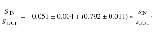
As expected, the entropy ratios are smaller than pseudo-entropy ratios, since projection effects smooth out the gradients.
In order to quantify the scatter around the best fit relation, we have
applied to the residuals a maximum likelihood algorithm that postulates
a parent distribution described by a mean and an intrinsic dispersion (Maccacaro et al. 1988). To do this we have calculated an ``effective error'' on the y coordinate, which takes into account the errors on both coordinates, defined as:
![]() ,
where b is the best-fit value for the slope of the linear relation between the two data sets (in this case b=0.792, Eq. (A.1)). The mean value of the residual distribution is consistent with zero (0.021), with an intrinsic dispersion
,
where b is the best-fit value for the slope of the linear relation between the two data sets (in this case b=0.792, Eq. (A.1)). The mean value of the residual distribution is consistent with zero (0.021), with an intrinsic dispersion
![]() .
.
![\begin{figure}
\par\includegraphics[width=8cm,clip]{13156a1.eps}
\end{figure}](/articles/aa/full_html/2010/02/aa13156-09/img161.png)
|
Figure A.1: Entropy ratio versus pseudo-entropy ratio. |
| Open with DEXTER | |
Appendix B: Figures of individual clusters
In this Appendix, we provide details for the low-entropy metal rich regions in the clusters with CC remnants. For each cluster, we show the EPIC X-ray flux image in the 0.4-2 keV energy range (see Rossetti et al. 2007, for details), the pseudo-entropy ratio image and the optical image taken from the DSS.
![\begin{figure}
\par\includegraphics[width=18cm,clip]{fig1.eps}
\end{figure}](/articles/aa/full_html/2010/02/aa13156-09/img162.png)
|
Figure B.1: Abell 1650. Upper left panel: X-ray flux image. Upper right panel: pseudo-entropy ratio map (zoom), with X-ray contours overlaid. Lower left panel: optical image (zoom), with X-ray contours overlaid. The red box in the first panel marks the region zoomed in in the other two panels. The red polygon in the other two panels is the contour of the ``CC-remnant'', i.e. it marks the bins where the pseudo-entropy ratio is <0.8. The green circle ( lower left) and ``X'' mark the position of the BCG. The scale refers to the pseudo-entropy ratio map. |
| Open with DEXTER | |
![\begin{figure}
\par\includegraphics[width=18cm,clip]{fig2.eps}
\end{figure}](/articles/aa/full_html/2010/02/aa13156-09/img163.png)
|
Figure B.2: MKW3s. Upper left panel: X-ray flux image. Upper right panel: pseudo-entropy ratio map (zoom), with X-ray contours overlaid. Lower left panel: optical image (zoom), with X-ray contours overlaid. The red box in the first panel marks the region zoomed in in the other two panels. The red polygon in the other two panels is the contour of the ``CC-remnant'', i.e. it marks the bins where the pseudo-entropy ratio is <0.8. The green circle ( lower left) and ``X'' mark the position of the BCG. The scale refers to the pseudo-entropy ratio map. |
| Open with DEXTER | |
![\begin{figure}
\par\includegraphics[width=18cm,clip]{fig3.eps}
\end{figure}](/articles/aa/full_html/2010/02/aa13156-09/img164.png)
|
Figure B.3: A4038. Upper left panel: X-ray flux image. Upper right panel: pseudo-entropy ratio map (zoom), with X-ray contours overlaid. Lower left panel: optical image (zoom), with X-ray contours overlaid. The red box in the first panel marks the region zoomed in in the other two panels. The red polygon in the other two panels is the contour of the ``CC-remnant'', i.e. it marks the bins where the pseudo-entropy ratio is <0.8. The green circle ( lower left) and ``X'' mark the position of the BCG. The scale refers to the pseudo-entropy ratio map. |
| Open with DEXTER | |
![\begin{figure}
\par\includegraphics[width=18cm,clip]{fig4.eps}
\end{figure}](/articles/aa/full_html/2010/02/aa13156-09/img165.png)
|
Figure B.4: A1644. Upper left panel: X-ray flux image. Upper right panel: pseudo-entropy ratio map (zoom), with X-ray contours overlaid. Lower left panel: optical image (zoom), with X-ray contours overlaid. The red box in the first panel marks the region zoomed in in the other two panels. The red polygon in the other two panels is the contour of the ``CC-remnant'', i.e. it marks the bins where the pseudo-entropy ratio is <0.8. The green circle ( lower left) and ``X'' mark the position of the BCG. The scale refers to the pseudo-entropy ratio map. |
| Open with DEXTER | |
![\begin{figure}
\par\includegraphics[width=18cm,clip]{fig5.eps}
\end{figure}](/articles/aa/full_html/2010/02/aa13156-09/img166.png)
|
Figure B.5: Abell 1689. Upper left panel: X-ray flux image. Upper right panel: pseudo-entropy ratio map (zoom), with X-ray contours overlaid. Lower left panel: optical image (zoom), with X-ray contours overlaid. The red box in the first panel marks the region zoomed in in the other two panels. The red polygon in the other two panels is the contour of the ``CC-remnant'', i.e. it marks the bins where the pseudo-entropy ratio is <0.8. The green circle ( lower left) and ``X'' mark the position of the BCG. The scale refers to the pseudo-entropy ratio map. |
| Open with DEXTER | |
![\begin{figure}
\par\includegraphics[width=18cm,clip]{fig6.eps}
\end{figure}](/articles/aa/full_html/2010/02/aa13156-09/img167.png)
|
Figure B.6: Abell 3558. Upper left panel: X-ray flux image. Upper right panel: pseudo-entropy ratio map (zoom), with X-ray contours overlaid. White regions have no data because of point sources subtraction (Rossetti et al. 2007). Lower left panel: optical image (zoom), with X-ray contours overlaid. The red box in the first panel marks the region zoomed in in the other two panels. The red polygon in the other two panels is the contour of the ``CC-remnant'', i.e. it marks the bins where the pseudo-entropy ratio is <0.8. The green circle ( lower left) and ``X'' mark the position of the BCG. The scale refers to the pseudo-entropy ratio map. |
| Open with DEXTER | |
![\begin{figure}
\par\includegraphics[width=18cm,clip]{fig7.eps}
\end{figure}](/articles/aa/full_html/2010/02/aa13156-09/img168.png)
|
Figure B.7: Abell 576. Upper left panel: X-ray flux image. Upper right panel: pseudo-entropy ratio map (zoom), with X-ray contours overlaid. Lower left panel: optical image (zoom), with X-ray contours overlaid. The red box in the first panel marks the region zoomed in in the other two panels. The red polygon in the other two panels is the contour of the ``CC-remnant'', i.e. it marks the bins where the pseudo-entropy ratio is <0.8. The green circle ( lower left) and ``X'' mark the position of the BCG. The scale refers to the pseudo-entropy ratio map. |
| Open with DEXTER | |
![\begin{figure}
\par\includegraphics[width=18cm,clip]{fig8.eps}
\end{figure}](/articles/aa/full_html/2010/02/aa13156-09/img169.png)
|
Figure B.8: Abell 754. Upper left panel: X-ray flux image. Upper right panel: pseudo-entropy ratio map (zoom), with X-ray contours overlaid. Lower left panel: optical image (zoom), with X-ray contours overlaid. The red box in the first panel marks the region zoomed in in the other two panels. The red polygon in the upper right panel is the contour of the ``CC-remnant'', i.e. it marks the bins where the pseudo-entropy ratio is <0.8. The blue circle and X show the position of the BCG, while the green circle and X show the elliptical galaxy 2MASSX J09091923-0941591. The scale refers to the pseudo-entropy ratio map. |
| Open with DEXTER | |
![\begin{figure}
\par\includegraphics[width=18cm,clip]{fig9.eps}
\end{figure}](/articles/aa/full_html/2010/02/aa13156-09/img170.png)
|
Figure B.9: Abell 3562. Upper left panel: X-ray flux image. Upper right panel: pseudo-entropy ratio map (zoom), with X-ray contours overlaid. Lower left panel: optical image (zoom), with X-ray contours overlaid. The red box in the first panel marks the region zoomed in in the other two panels. The red polygon in the other two panels is the contour of the ``CC-remnant'', i.e. it marks the bins where the pseudo-entropy ratio is <0.8. The green circle ( lower left) and ``X'' mark the position of the BCG. The scale refers to the pseudo-entropy ratio map. |
| Open with DEXTER | |
![\begin{figure}
\par\includegraphics[width=18cm,clip]{fig10.eps}
\end{figure}](/articles/aa/full_html/2010/02/aa13156-09/img171.png)
|
Figure B.10: Abell 3571. Upper left panel: X-ray flux image. Upper right panel: pseudo-entropy ratio map (zoom), with X-ray contours overlaid. Lower left panel: optical image (zoom), with X-ray contours overlaid. The red box in the first panel marks the region zoomed in in the other two panels. The red polygon in the other two panels is the contour of the ``CC-remnant'', i.e. it marks the bins where the pseudo-entropy ratio is <0.8. The green circle ( lower left) and ``X'' mark the position of the BCG. The scale refers to the pseudo-entropy ratio map. |
| Open with DEXTER | |
![\begin{figure}
\par\includegraphics[width=18cm,clip]{fig11.eps}
\end{figure}](/articles/aa/full_html/2010/02/aa13156-09/img172.png)
|
Figure B.11: Abell 3667. Upper left panel: X-ray flux image. Upper right panel: pseudo entropy ratio map (zoom), with X-ray contours overlaid. Lower left panel: optical image (zoom), with X-ray contours overlaid. The red box in the first panel marks the region zoomed in in the other two panels. The red polygon in the other two panels is the contour of the ``CC-remnant'', i.e. it marks the bins where the pseudo entropy ratio is <0.8. The yellow circle ( lower left) and ``X'' mark the position of the BCG. The scale refers to the pseudo entropy ratio map. |
| Open with DEXTER | |
![\begin{figure}
\par\includegraphics[width=18cm,clip]{fig12.eps}
\end{figure}](/articles/aa/full_html/2010/02/aa13156-09/img173.png)
|
Figure B.12: Abell 2256. Upper left panel: X-ray flux image. Upper right panel: pseudo-entropy ratio map (zoom), with X-ray contours overlaid. Lower left panel: optical image (zoom), with X-ray contours overlaid. The red box in the first panel marks the region zoomed in in the other two panels. The red polygon in the other two panels is the contour of the ``CC-remnant'', i.e. it marks the bins where the pseudo-entropy ratio is <0.8. The green circle ( lower left) and ``X'' mark the position of the BCG. The scale refers to the pseudo-entropy ratio map. |
| Open with DEXTER | |
Footnotes
- ... clusters
- Appendices are only available in electronic form at http://www.aanda.org
- ... value
- The only exception is A478, where we found a difference of
about a factor of two between the galactic value (1.48

 ,
Dickey & Lockman 1990) and the best fit value (2.7
).
,
Dickey & Lockman 1990) and the best fit value (2.7
).
- ... abundance
- For solar abundances we refer to Anders & Grevesse (1989).
- ... ratio
- X-ray astronomers usually define as ``entropy''
the quantity
 ,
where
,
where  is
the electronic density and
is
the electronic density and  the deprojected temperature of the ICM (Ponman
et al. 1999). In this paper, we use the definition
of ``pseudo-entropy''
the deprojected temperature of the ICM (Ponman
et al. 1999). In this paper, we use the definition
of ``pseudo-entropy''  ,
where T is the projected temperature and EM is
the emission measure, i.e. the normalization of the MEKAL
model in XSPEC per units of area (see Rossetti
et al. 2007, for more details).
,
where T is the projected temperature and EM is
the emission measure, i.e. the normalization of the MEKAL
model in XSPEC per units of area (see Rossetti
et al. 2007, for more details).
- ... remnants''
- The term ``remnant of cool cores'' has been recently used by Fusco-Femiano et al. (2009) to describe structures similar to the ones we detect albeit without information on the metal abundance.
- ... FITEXY.PRO
- http://idlastro.gsfc.nasa.gov/ftp/pro/math/fitexy.pro
All Tables
Table 2: Properties of the clusters in the sample: the first 14 entries are LEC clusters, while the remaining are non-LEC.
Table 3: Properties of low entropy regions: clsters in Italics are ``AGN CC-remnants'', while clusters in bold type are ``merger CC-remnants''.
Table 1: Observations analyzed for the clusters in the sample.
All Figures
|
|
Figure 1:
Comparison of temperature and emission measure ratios for the clusters
in our sample. The solid line represents the threshold used to divide
clusters between low entropy clusters and non-low entropy clusters,
corresponding to
|
| Open with DEXTER | |
| In the text | |
|
|
Figure 2:
Upper panel: metal abundance profiles of LEC clusters as a
function of the pseudo-entropy ratio, in the regions of spectral
extraction. The symbols and colors are as in Table 1. Lower panel:
mean error weighted abundance profile for LEC clusters. Error bars
show the (small) error on the average, while dotted lines show the |
| Open with DEXTER | |
| In the text | |
|
|
Figure 3:
Metal abundance in the regions selected for spectral analysis for the 21 non-LEC objects in the sample ( upper panel) and as a function of the pseudo-entropy ratio in the regions ( lower panel). The horizontal line represents the reference value for the metalicity of outer regions of galaxy clusters
|
| Open with DEXTER | |
| In the text | |
|
|
Figure 4: Error weighted metal
abundance profile as a function of the pseudo entropy ratios for
LEC clusters (blue squares) and for the four clusters with low
central entropy (red circles). Dotted lines show the one |
| Open with DEXTER | |
| In the text | |
|
|
Figure 5:
Error weighted metal abundance profile as a function of the pseudo
entropy ratios for LEC clusters (blue squares) and for the
clusters with merger CC remnants (black circles). Dotted lines
show the one |
| Open with DEXTER | |
| In the text | |
|
|
Figure 6:
Metal abundance profiles of non-LEC clusters as a function of the
pseudo-entropy ratio in the regions of spectral extraction.
The symbols and colors are as in Table 1. The dashed horizontal line indicates the mean value of outer regions of galaxy clusters
|
| Open with DEXTER | |
| In the text | |
|
|
Figure 7: Cooling time in the inner 0.05 R180 for the clusters of the sample for which we have performed radial analysis and de-projection. Horizontal dashed line is the Hubble time. |
| Open with DEXTER | |
| In the text | |
|
|
Figure A.1: Entropy ratio versus pseudo-entropy ratio. |
| Open with DEXTER | |
| In the text | |
|
|
Figure B.1: Abell 1650. Upper left panel: X-ray flux image. Upper right panel: pseudo-entropy ratio map (zoom), with X-ray contours overlaid. Lower left panel: optical image (zoom), with X-ray contours overlaid. The red box in the first panel marks the region zoomed in in the other two panels. The red polygon in the other two panels is the contour of the ``CC-remnant'', i.e. it marks the bins where the pseudo-entropy ratio is <0.8. The green circle ( lower left) and ``X'' mark the position of the BCG. The scale refers to the pseudo-entropy ratio map. |
| Open with DEXTER | |
| In the text | |
|
|
Figure B.2: MKW3s. Upper left panel: X-ray flux image. Upper right panel: pseudo-entropy ratio map (zoom), with X-ray contours overlaid. Lower left panel: optical image (zoom), with X-ray contours overlaid. The red box in the first panel marks the region zoomed in in the other two panels. The red polygon in the other two panels is the contour of the ``CC-remnant'', i.e. it marks the bins where the pseudo-entropy ratio is <0.8. The green circle ( lower left) and ``X'' mark the position of the BCG. The scale refers to the pseudo-entropy ratio map. |
| Open with DEXTER | |
| In the text | |
|
|
Figure B.3: A4038. Upper left panel: X-ray flux image. Upper right panel: pseudo-entropy ratio map (zoom), with X-ray contours overlaid. Lower left panel: optical image (zoom), with X-ray contours overlaid. The red box in the first panel marks the region zoomed in in the other two panels. The red polygon in the other two panels is the contour of the ``CC-remnant'', i.e. it marks the bins where the pseudo-entropy ratio is <0.8. The green circle ( lower left) and ``X'' mark the position of the BCG. The scale refers to the pseudo-entropy ratio map. |
| Open with DEXTER | |
| In the text | |
|
|
Figure B.4: A1644. Upper left panel: X-ray flux image. Upper right panel: pseudo-entropy ratio map (zoom), with X-ray contours overlaid. Lower left panel: optical image (zoom), with X-ray contours overlaid. The red box in the first panel marks the region zoomed in in the other two panels. The red polygon in the other two panels is the contour of the ``CC-remnant'', i.e. it marks the bins where the pseudo-entropy ratio is <0.8. The green circle ( lower left) and ``X'' mark the position of the BCG. The scale refers to the pseudo-entropy ratio map. |
| Open with DEXTER | |
| In the text | |
|
|
Figure B.5: Abell 1689. Upper left panel: X-ray flux image. Upper right panel: pseudo-entropy ratio map (zoom), with X-ray contours overlaid. Lower left panel: optical image (zoom), with X-ray contours overlaid. The red box in the first panel marks the region zoomed in in the other two panels. The red polygon in the other two panels is the contour of the ``CC-remnant'', i.e. it marks the bins where the pseudo-entropy ratio is <0.8. The green circle ( lower left) and ``X'' mark the position of the BCG. The scale refers to the pseudo-entropy ratio map. |
| Open with DEXTER | |
| In the text | |
|
|
Figure B.6: Abell 3558. Upper left panel: X-ray flux image. Upper right panel: pseudo-entropy ratio map (zoom), with X-ray contours overlaid. White regions have no data because of point sources subtraction (Rossetti et al. 2007). Lower left panel: optical image (zoom), with X-ray contours overlaid. The red box in the first panel marks the region zoomed in in the other two panels. The red polygon in the other two panels is the contour of the ``CC-remnant'', i.e. it marks the bins where the pseudo-entropy ratio is <0.8. The green circle ( lower left) and ``X'' mark the position of the BCG. The scale refers to the pseudo-entropy ratio map. |
| Open with DEXTER | |
| In the text | |
|
|
Figure B.7: Abell 576. Upper left panel: X-ray flux image. Upper right panel: pseudo-entropy ratio map (zoom), with X-ray contours overlaid. Lower left panel: optical image (zoom), with X-ray contours overlaid. The red box in the first panel marks the region zoomed in in the other two panels. The red polygon in the other two panels is the contour of the ``CC-remnant'', i.e. it marks the bins where the pseudo-entropy ratio is <0.8. The green circle ( lower left) and ``X'' mark the position of the BCG. The scale refers to the pseudo-entropy ratio map. |
| Open with DEXTER | |
| In the text | |
|
|
Figure B.8: Abell 754. Upper left panel: X-ray flux image. Upper right panel: pseudo-entropy ratio map (zoom), with X-ray contours overlaid. Lower left panel: optical image (zoom), with X-ray contours overlaid. The red box in the first panel marks the region zoomed in in the other two panels. The red polygon in the upper right panel is the contour of the ``CC-remnant'', i.e. it marks the bins where the pseudo-entropy ratio is <0.8. The blue circle and X show the position of the BCG, while the green circle and X show the elliptical galaxy 2MASSX J09091923-0941591. The scale refers to the pseudo-entropy ratio map. |
| Open with DEXTER | |
| In the text | |
|
|
Figure B.9: Abell 3562. Upper left panel: X-ray flux image. Upper right panel: pseudo-entropy ratio map (zoom), with X-ray contours overlaid. Lower left panel: optical image (zoom), with X-ray contours overlaid. The red box in the first panel marks the region zoomed in in the other two panels. The red polygon in the other two panels is the contour of the ``CC-remnant'', i.e. it marks the bins where the pseudo-entropy ratio is <0.8. The green circle ( lower left) and ``X'' mark the position of the BCG. The scale refers to the pseudo-entropy ratio map. |
| Open with DEXTER | |
| In the text | |
|
|
Figure B.10: Abell 3571. Upper left panel: X-ray flux image. Upper right panel: pseudo-entropy ratio map (zoom), with X-ray contours overlaid. Lower left panel: optical image (zoom), with X-ray contours overlaid. The red box in the first panel marks the region zoomed in in the other two panels. The red polygon in the other two panels is the contour of the ``CC-remnant'', i.e. it marks the bins where the pseudo-entropy ratio is <0.8. The green circle ( lower left) and ``X'' mark the position of the BCG. The scale refers to the pseudo-entropy ratio map. |
| Open with DEXTER | |
| In the text | |
|
|
Figure B.11: Abell 3667. Upper left panel: X-ray flux image. Upper right panel: pseudo entropy ratio map (zoom), with X-ray contours overlaid. Lower left panel: optical image (zoom), with X-ray contours overlaid. The red box in the first panel marks the region zoomed in in the other two panels. The red polygon in the other two panels is the contour of the ``CC-remnant'', i.e. it marks the bins where the pseudo entropy ratio is <0.8. The yellow circle ( lower left) and ``X'' mark the position of the BCG. The scale refers to the pseudo entropy ratio map. |
| Open with DEXTER | |
| In the text | |
|
|
Figure B.12: Abell 2256. Upper left panel: X-ray flux image. Upper right panel: pseudo-entropy ratio map (zoom), with X-ray contours overlaid. Lower left panel: optical image (zoom), with X-ray contours overlaid. The red box in the first panel marks the region zoomed in in the other two panels. The red polygon in the other two panels is the contour of the ``CC-remnant'', i.e. it marks the bins where the pseudo-entropy ratio is <0.8. The green circle ( lower left) and ``X'' mark the position of the BCG. The scale refers to the pseudo-entropy ratio map. |
| Open with DEXTER | |
| In the text | |
Copyright ESO 2010
Current usage metrics show cumulative count of Article Views (full-text article views including HTML views, PDF and ePub downloads, according to the available data) and Abstracts Views on Vision4Press platform.
Data correspond to usage on the plateform after 2015. The current usage metrics is available 48-96 hours after online publication and is updated daily on week days.
Initial download of the metrics may take a while.