Online Material

Appendix A: Relation between pseudo-entropy and entropy ratios

We have used the entropy profiles for the 31 clusters in our sample for which we have performed radial analysis to test if the pseudo-entropy ratios (defined in Paper I) are good indicators of the behavior of the true three dimensional entropy ( $S\equiv T_{\rm X}/n_{\rm e}^{2/3}$ ). We have therefore calculated the entropy ratio $S_{\rm IN}/S_{\rm OUT}$ , starting from the three-dimensional entropy profiles obtained with the de-projected temperature and density profiles. We show in Fig. A.1 that there is a strong correlation between the ``true'' entropy ratio and the ``pseudo'' entropy ratios. We fitted the points in Fig. A.1 with a linear model taking into account the errors on both coordinates (with the IDL Astrolib procedure FITEXY.PRO), and we found

$\begin{displaymath}% \frac{S_{\rm IN}}{S_{\rm OUT}}=-0.051\pm0.004+(0.792 \pm 0.011)*\frac{s_{\rm IN}}{s_{\rm OUT}}\cdot \end{displaymath}$

(A.1)

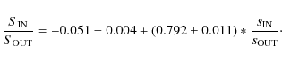
As expected, the entropy ratios are smaller than pseudo-entropy ratios, since projection effects smooth out the gradients.

In order to quantify the scatter around the best fit relation, we have applied to the residuals a maximum likelihood algorithm that postulates a parent distribution described by a mean and an intrinsic dispersion (Maccacaro et al. 1988). To do this we have calculated an ``effective error'' on the y coordinate, which takes into account the errors on both coordinates, defined as: $\sigma_{\rm eff}^2=\sigma_y^2+b^2\sigma_x^2$ , where b is the best-fit value for the slope of the linear relation between the two data sets (in this case b=0.792, Eq. (A.1)). The mean value of the residual distribution is consistent with zero (0.021), with an intrinsic dispersion $\sigma=0.043$ .

$\begin{figure} \par\includegraphics[width=8cm,clip]{13156a1.eps} \end{figure}$	Figure A.1: Entropy ratio versus pseudo-entropy ratio.
Open with DEXTER

Appendix B: Figures of individual clusters

In this Appendix, we provide details for the low-entropy metal rich regions in the clusters with CC remnants. For each cluster, we show the EPIC X-ray flux image in the 0.4-2 keV energy range (see Rossetti et al. 2007, for details), the pseudo-entropy ratio image and the optical image taken from the DSS.

$\begin{figure} \par\includegraphics[width=18cm,clip]{fig1.eps} \end{figure}$

Figure B.1:

Abell 1650. Upper left panel: X-ray flux image. Upper right panel: pseudo-entropy ratio map (zoom), with X-ray contours overlaid. Lower left panel: optical image (zoom), with X-ray contours overlaid. The red box in the first panel marks the region zoomed in in the other two panels. The red polygon in the other two panels is the contour of the ``CC-remnant'', i.e. it marks the bins where the pseudo-entropy ratio is <0.8. The green circle ( lower left) and ``X'' mark the position of the BCG. The scale refers to the pseudo-entropy ratio map.

Open with DEXTER

$\begin{figure} \par\includegraphics[width=18cm,clip]{fig2.eps} \end{figure}$

Figure B.2:

MKW3s. Upper left panel: X-ray flux image. Upper right panel: pseudo-entropy ratio map (zoom), with X-ray contours overlaid. Lower left panel: optical image (zoom), with X-ray contours overlaid. The red box in the first panel marks the region zoomed in in the other two panels. The red polygon in the other two panels is the contour of the ``CC-remnant'', i.e. it marks the bins where the pseudo-entropy ratio is <0.8. The green circle ( lower left) and ``X'' mark the position of the BCG. The scale refers to the pseudo-entropy ratio map.

Open with DEXTER

$\begin{figure} \par\includegraphics[width=18cm,clip]{fig3.eps} \end{figure}$

Figure B.3:

A4038. Upper left panel: X-ray flux image. Upper right panel: pseudo-entropy ratio map (zoom), with X-ray contours overlaid. Lower left panel: optical image (zoom), with X-ray contours overlaid. The red box in the first panel marks the region zoomed in in the other two panels. The red polygon in the other two panels is the contour of the ``CC-remnant'', i.e. it marks the bins where the pseudo-entropy ratio is <0.8. The green circle ( lower left) and ``X'' mark the position of the BCG. The scale refers to the pseudo-entropy ratio map.

Open with DEXTER

$\begin{figure} \par\includegraphics[width=18cm,clip]{fig4.eps} \end{figure}$

Figure B.4:

A1644. Upper left panel: X-ray flux image. Upper right panel: pseudo-entropy ratio map (zoom), with X-ray contours overlaid. Lower left panel: optical image (zoom), with X-ray contours overlaid. The red box in the first panel marks the region zoomed in in the other two panels. The red polygon in the other two panels is the contour of the ``CC-remnant'', i.e. it marks the bins where the pseudo-entropy ratio is <0.8. The green circle ( lower left) and ``X'' mark the position of the BCG. The scale refers to the pseudo-entropy ratio map.

Open with DEXTER

$\begin{figure} \par\includegraphics[width=18cm,clip]{fig5.eps} \end{figure}$

Figure B.5:

Abell 1689. Upper left panel: X-ray flux image. Upper right panel: pseudo-entropy ratio map (zoom), with X-ray contours overlaid. Lower left panel: optical image (zoom), with X-ray contours overlaid. The red box in the first panel marks the region zoomed in in the other two panels. The red polygon in the other two panels is the contour of the ``CC-remnant'', i.e. it marks the bins where the pseudo-entropy ratio is <0.8. The green circle ( lower left) and ``X'' mark the position of the BCG. The scale refers to the pseudo-entropy ratio map.

Open with DEXTER

$\begin{figure} \par\includegraphics[width=18cm,clip]{fig6.eps} \end{figure}$

Figure B.6:

Abell 3558. Upper left panel: X-ray flux image. Upper right panel: pseudo-entropy ratio map (zoom), with X-ray contours overlaid. White regions have no data because of point sources subtraction (Rossetti et al. 2007). Lower left panel: optical image (zoom), with X-ray contours overlaid. The red box in the first panel marks the region zoomed in in the other two panels. The red polygon in the other two panels is the contour of the ``CC-remnant'', i.e. it marks the bins where the pseudo-entropy ratio is <0.8. The green circle ( lower left) and ``X'' mark the position of the BCG. The scale refers to the pseudo-entropy ratio map.

Open with DEXTER

$\begin{figure} \par\includegraphics[width=18cm,clip]{fig7.eps} \end{figure}$

Figure B.7:

Abell 576. Upper left panel: X-ray flux image. Upper right panel: pseudo-entropy ratio map (zoom), with X-ray contours overlaid. Lower left panel: optical image (zoom), with X-ray contours overlaid. The red box in the first panel marks the region zoomed in in the other two panels. The red polygon in the other two panels is the contour of the ``CC-remnant'', i.e. it marks the bins where the pseudo-entropy ratio is <0.8. The green circle ( lower left) and ``X'' mark the position of the BCG. The scale refers to the pseudo-entropy ratio map.

Open with DEXTER

$\begin{figure} \par\includegraphics[width=18cm,clip]{fig8.eps} \end{figure}$

Figure B.8:

Abell 754. Upper left panel: X-ray flux image. Upper right panel: pseudo-entropy ratio map (zoom), with X-ray contours overlaid. Lower left panel: optical image (zoom), with X-ray contours overlaid. The red box in the first panel marks the region zoomed in in the other two panels. The red polygon in the upper right panel is the contour of the ``CC-remnant'', i.e. it marks the bins where the pseudo-entropy ratio is <0.8. The blue circle and X show the position of the BCG, while the green circle and X show the elliptical galaxy 2MASSX J09091923-0941591. The scale refers to the pseudo-entropy ratio map.

Open with DEXTER

$\begin{figure} \par\includegraphics[width=18cm,clip]{fig9.eps} \end{figure}$

Figure B.9:

Abell 3562. Upper left panel: X-ray flux image. Upper right panel: pseudo-entropy ratio map (zoom), with X-ray contours overlaid. Lower left panel: optical image (zoom), with X-ray contours overlaid. The red box in the first panel marks the region zoomed in in the other two panels. The red polygon in the other two panels is the contour of the ``CC-remnant'', i.e. it marks the bins where the pseudo-entropy ratio is <0.8. The green circle ( lower left) and ``X'' mark the position of the BCG. The scale refers to the pseudo-entropy ratio map.

Open with DEXTER

$\begin{figure} \par\includegraphics[width=18cm,clip]{fig10.eps} \end{figure}$

Figure B.10:

Abell 3571. Upper left panel: X-ray flux image. Upper right panel: pseudo-entropy ratio map (zoom), with X-ray contours overlaid. Lower left panel: optical image (zoom), with X-ray contours overlaid. The red box in the first panel marks the region zoomed in in the other two panels. The red polygon in the other two panels is the contour of the ``CC-remnant'', i.e. it marks the bins where the pseudo-entropy ratio is <0.8. The green circle ( lower left) and ``X'' mark the position of the BCG. The scale refers to the pseudo-entropy ratio map.

Open with DEXTER

$\begin{figure} \par\includegraphics[width=18cm,clip]{fig11.eps} \end{figure}$

Figure B.11:

Abell 3667. Upper left panel: X-ray flux image. Upper right panel: pseudo entropy ratio map (zoom), with X-ray contours overlaid. Lower left panel: optical image (zoom), with X-ray contours overlaid. The red box in the first panel marks the region zoomed in in the other two panels. The red polygon in the other two panels is the contour of the ``CC-remnant'', i.e. it marks the bins where the pseudo entropy ratio is <0.8. The yellow circle ( lower left) and ``X'' mark the position of the BCG. The scale refers to the pseudo entropy ratio map.

Open with DEXTER

$\begin{figure} \par\includegraphics[width=18cm,clip]{fig12.eps} \end{figure}$

Figure B.12:

Abell 2256. Upper left panel: X-ray flux image. Upper right panel: pseudo-entropy ratio map (zoom), with X-ray contours overlaid. Lower left panel: optical image (zoom), with X-ray contours overlaid. The red box in the first panel marks the region zoomed in in the other two panels. The red polygon in the other two panels is the contour of the ``CC-remnant'', i.e. it marks the bins where the pseudo-entropy ratio is <0.8. The green circle ( lower left) and ``X'' mark the position of the BCG. The scale refers to the pseudo-entropy ratio map.

Open with DEXTER