| Issue |
A&A
Volume 509, January 2010
|
|
|---|---|---|
| Article Number | A25 | |
| Number of page(s) | 10 | |
| Section | Galactic structure, stellar clusters, and populations | |
| DOI | https://doi.org/10.1051/0004-6361/200913381 | |
| Published online | 12 January 2010 | |
Determination of the local dark matter density in our Galaxy
M. Weber - W. de Boer
Institut für Experimentelle Kernphysik, Karlsruher Insitut für Technologie (KIT), PO Box 6980, 76128 Karlsruhe, Germany
Received 30 September 2009 / Accepted 9 October 2009
Abstract
Context. The rotation curve, the total mass and the
gravitational potential of the Galaxy are sensitive measurements of the
dark matter halo profile.
Aims. Cuspy and cored DM halo profiles are analysed
with respect to recent astronomical constraints in order to constrain
the shape of the Galactic DM halo and the local DM density.
Methods. All Galactic density components (luminous
matter and DM) are parametrized. Then the total density distribution is
constrained by astronomical observations: 1) the total mass of the
Galaxy, 2) the total matter density at the position of the Sun, 3) the
surface density of the visible matter, 4) the surface density of the
total matter in the vicinity of the Sun, 5) the rotation speed of the
Sun and 6) the shape of the velocity distribution within and above the
Galactic disc. The mass model of the Galaxy is mainly constrained by
the local matter density (Oort limit), the rotation speed of the Sun
and the total mass of the Galaxy from tracer stars in the halo.
Results. We showed from a statistical ![]() fit to all data that the local DM density is strongly positively
(negatively) correlated with the scale length of the DM halo (baryonic
disc). Since these scale lengths are poorly constrained the local DM
density can vary from 0.2 to 0.4 GeV cm-3
(
fit to all data that the local DM density is strongly positively
(negatively) correlated with the scale length of the DM halo (baryonic
disc). Since these scale lengths are poorly constrained the local DM
density can vary from 0.2 to 0.4 GeV cm-3
(
![]() pc-3)
for a spherical DM halo profile and allowing total Galaxy masses up to
pc-3)
for a spherical DM halo profile and allowing total Galaxy masses up to ![]() .
For oblate DM haloes and dark matter discs, as predicted in recent N-body
simulations, the local DM density can be increased significantly.
.
For oblate DM haloes and dark matter discs, as predicted in recent N-body
simulations, the local DM density can be increased significantly.
Key words: Galaxy: halo - Galaxy: structure - Galaxy: kinematics and dynamics - Galaxy: fundamental parameters - Galaxy: general
1 Introduction
The best evidence for dark matter (DM) in galaxies is usually provided by rotation curves, which do not fall off fast enough at large distances from the centre. This can be understood, either by assuming Newton's law of gravitation is not valid at large distances, the so-called MOND (modified newtonian dynamics) theory (Bekenstein & Milgrom 1984; Bienayme et al. 2009), or the visible mass distribution is augmented by invisible mass, i.e. DM. For a flat rotation curve the DM density has to fall off like 1/r2 at large distances.
Given the overwhelming evidence for DM on all scales from the flatness of the universe combined with gravitational lensing and structure formation we assume DM exists and try to constrain the DM density from dynamical constraints, for which better data became available in recent years:
- 1.
- the total mass of the Galaxy has to be about 1012 solar masses (Xue et al. 2008; Wilkinson & Evans 1999; Battaglia et al. 2005);
- 2.
- the total mass inside the solar orbit is constrained by the well-known rotation speed of the solar system;
- 3.
- the total matter density at the position of the Sun from the gravitational potential determined from the movements of local stars as measured with the Hipparcos satellite (Holmberg & Flynn 2004);
- 4.
- the surface density of the visible matter at the position of the Sun (Naab & Ostriker 2006, and references therein);
- 5.
- the surface density of the total matter at the position of the Sun (Holmberg & Flynn 2004; Bienayme et al. 2005; Kuijken & Gilmore 1991);
- 6.
- the shape of the rotation curve within Galactic disc (Sofue et al. 2008, and references therein);
- 7.
- the velocity distribution above the Galactic disc (z>4 kpc) (Xue et al. 2008).
Such substructure will not be investigated in this paper, but smooth DM haloes with different (cored and cuspy) profiles will be compared with all available data. These will result in lower limits on the local DM density, since dark matter discs or other local substructure will only enhance the local density.
A reliable determination of the local DM density is of great interest for direct DM search experiments, where elastic collisions between WIMPs and the target material of the detector are searched for. This signal is proportional to the local density. A review on direct searches can be found in the paper by Spooner (2007).
The structure of the paper is as follows: in Sect. 2 the
parametrization of the luminous matter and five different DM halo
profiles
are given. In Sect. 3
the experimental data used to determine the mass model are discussed.
Then the
numerical determination of the mass model parameters using a ![]() fit
of all dynamical constraints is discussed in Sect. 4.
At the end a summary of the results is given.
fit
of all dynamical constraints is discussed in Sect. 4.
At the end a summary of the results is given.
2 Parametrization of the density distributions
In order to constrain the mass model of the Galaxy by data it is convenient to have a parametrization for both, the visible an dark matter density. These parametrizations are introduced here.
2.1 Parametrization of the luminous matter density
The density distribution of the luminous matter of a spiral galaxy is
split into two parts,
the Galactic disc and the Galactic bulge. The parametrization of
the density distribution of the bulge is adapted from
the publication by Cardone
& Sereno (2005)
For a good description of the RC near the GC the parameters of the bulge profile are found to be
The stellar contribution of the Galactic disc is split into two discs - a thin and a thick disc - which are usually parametrized by an exponentially decreasing density distribution.
The parametrization of the Galactic disc is taken from the
publication
by Sparke (2007)
The parameter
There is some freedom in the choice of the parameters for the
Galactic disc. Its density in the
GC is, as in case of the bulge, unknown, so it has to be a free
parameter. For the scale radius we adopt the value from Hammer et al. (2007)
The scale height
The parametrization of the visible mass discussed above
leads to a mass of the Galactic bulge of about ![]() .
The mass of the Galactic disc varies for different fits because of the
variation of the parameters
.
The mass of the Galactic disc varies for different fits because of the
variation of the parameters ![]() and
and ![]() .
It is in the range of
.
It is in the range of
![]() to
to ![]() solar masses.
In addition to the luminous matter the density profile of the DM halo
has to be parametrized. This is discussed in the following section.
solar masses.
In addition to the luminous matter the density profile of the DM halo
has to be parametrized. This is discussed in the following section.
2.2 Parameterization of the dark matter density
The first analytical analysis of
structure formation in the Universe by Gunn
(1977)
predicted that DM in Galactic haloes are distributed according to a
simple power law distribution ![]() .
However,
later studies based on numerical N-body simulations
(Navarro
et al. 1997; Moore et al. 1999)
found that the slope of the density distribution in the DM halo is
different for different distances from the GC. Today it is commonly
believed that the profile of a DM halo can be well fitted by the
universal function
.
However,
later studies based on numerical N-body simulations
(Navarro
et al. 1997; Moore et al. 1999)
found that the slope of the density distribution in the DM halo is
different for different distances from the GC. Today it is commonly
believed that the profile of a DM halo can be well fitted by the
universal function
|
|
= | 
|
(4) |
| = | 
|
Here, a is the scale radius of the density profile, which determines at what distance from the centre the slope of the profile changes,
In contrast to cuspy profiles the density distributions
preferred by observations of rotation curves
of low surface brightness galaxies and dwarf spiral galaxies have a
nearly constant DM density in the GC (
![]() )
(Oh
et al. 2008; Gentile et al. 2007;
Salucci
et al. 2007).
Such profiles are called ``cored'' profiles
due to the constant density in the kpc scale in the central region.
Two different cored halo profiles are considered in this analysis. The
first profile is called
pseudo-isothermal profile (hereafter PISO) since it is an isothermal
profile
(
)
(Oh
et al. 2008; Gentile et al. 2007;
Salucci
et al. 2007).
Such profiles are called ``cored'' profiles
due to the constant density in the kpc scale in the central region.
Two different cored halo profiles are considered in this analysis. The
first profile is called
pseudo-isothermal profile (hereafter PISO) since it is an isothermal
profile
(![]() r-2)
which is flattened in the centre.
The second cored halo profile (hereafter 240) is similar to the PISO
profile but decreases
faster for large radii. The parameter settings
of the several density profiles are shown in Table 1.
The local DM density
r-2)
which is flattened in the centre.
The second cored halo profile (hereafter 240) is similar to the PISO
profile but decreases
faster for large radii. The parameter settings
of the several density profiles are shown in Table 1.
The local DM density ![]() is a priori an unknown parameter
and therefore a degree of freedom in the density model. In the
publications by Gates
et al. (1995); Amsler et al. (2008)
its value
is quoted to be in the range 0.2-0.7 GeV cm-3
(0.005-0.018
is a priori an unknown parameter
and therefore a degree of freedom in the density model. In the
publications by Gates
et al. (1995); Amsler et al. (2008)
its value
is quoted to be in the range 0.2-0.7 GeV cm-3
(0.005-0.018 ![]() pc-3).
In this analysis
pc-3).
In this analysis ![]() is left free. In
Fig. 1
the different profiles are shown for equal
masses within the solar orbit.
is left free. In
Fig. 1
the different profiles are shown for equal
masses within the solar orbit.
Table 1: Parameter settings for the different DM halo profiles considered in this analysis.
![\begin{figure}
\par\includegraphics[width=9cm,clip]{13381fg1.eps}
\end{figure}](/articles/aa/full_html/2010/01/aa13381-09/img56.png)
|
Figure 1:
Radial DM density distribution for the parameters given in
Table 1.
The normalization |
| Open with DEXTER | |
3 Dynamical constraints on the mass model of the Milky Way
As mentioned in the introduction the mass model of the Galaxy is
largely constrained by the total mass of the Galaxy, the rotation
velocity of the Sun at its orbital radius ![]() and the local matter
density
and the local matter
density ![]() (
(![]() ), known as
the Oort limit. An additional constraint comes from the local
surface density. The experimental input for these constraints
is discussed first.
), known as
the Oort limit. An additional constraint comes from the local
surface density. The experimental input for these constraints
is discussed first.
3.1 Total mass
The total mass of the MW is an important quantity in order to constrain the DM density distribution. In general, it is measured indirectly either via the kinematics of distant halo tracer stars or satellite galaxies or the vertical scale height of the gas distribution of the Galactic disc, which can be measured at large distances from the GC.
The definition of the total mass of the Galaxy is difficult since a slowly decreasing density has an infinite extension. The total mass of a galaxy is conventionally defined as the mass within the so-called virial radius. At this radius the total mass of the accumulated density of the MW is equal to the mass of a homogeneous sphere with the constant density of 200 times the critical density of the Universe.
In the paper by Wilkinson
& Evans (1999) the mass of the MW was
estimated from measurements of the radial velocities of 27
globular clusters and satellite galaxies for Galactocentric
distances R > 20 kpc, using a
Bayesian likelihood method and
a spherical halo mass model with a truncated radius. They found
a mass of the Galaxy within 50 kpc of ![]() and a total mass of
and a total mass of
![]() .
A similar
analysis was done with more tracer stars by
Sakamoto et al. (2003);
they find
.
A similar
analysis was done with more tracer stars by
Sakamoto et al. (2003);
they find ![]() .
These measurements used a simple
parametrization of the potential. Analyses using an NFW profile
for the DM distribution usually find a lower total mass, given
it steeper fall-off of the density profile at large distances.
.
These measurements used a simple
parametrization of the potential. Analyses using an NFW profile
for the DM distribution usually find a lower total mass, given
it steeper fall-off of the density profile at large distances.
Using a large sample of 2400 blue horizontal-branch
(BHB) tracer stars from the Sloan Digital Sky Survey (SDSS) in the
halo (z > 4 kpc, R<60 kpc)
and comparing the results with
N-body simulations using an NFW profile Xue et al. (2008) find
which corresponds to
Figure 2
shows the radial dependence of the
total Galactic mass for the different spherical halo profiles. At small
radii r <5 kpc the density
distribution is dominated by the luminous
matter, shown by the thin solid line, which is independent of the halo
profile. The mass of a homogeneous sphere with 200 times the critical
density of the Universe is also shown. The crossing of a mass
distribution with this line defines the total Galactic
mass and the virial radius for this density distribution which is
210 kpc
for a Galactic mass of ![]() .
.
The mass distributions of the NFW and the BE profile are quite
similar since these profiles differ only in the region around
the GC where the influence of DM is small. The 240 profile yields the
smallest
mass while the mass distribution of the PISO profile shows a linear
increase with radius. The reason is the quadratic decrease
(![]() r-2)
of the PISO profile. Consequently, the integral
of such a profile leads to a linear increase of the Galactic mass.
By going from spherical to elliptical profiles the mass
can be changed significantly, as will be discussed later.
r-2)
of the PISO profile. Consequently, the integral
of such a profile leads to a linear increase of the Galactic mass.
By going from spherical to elliptical profiles the mass
can be changed significantly, as will be discussed later.
![\begin{figure}
\par\includegraphics[width=9cm,clip]{13381fg2.eps}
\par\end{figure}](/articles/aa/full_html/2010/01/aa13381-09/img67.png)
|
Figure 2:
The mass inside a radius as function of that radius is shown for the
different halo profiles defined in Table 1. The thin
solid line represents the visible mass which is different for different
halo profiles because of the variation of the parameters |
| Open with DEXTER | |
![\begin{figure}
\par\mbox{\subfigure[Rotation curve ($z = 0$\space kpc), non-aver...
...eraged]{\includegraphics[width=9cm,angle=0,clip]{13381fg4.eps} }}
\end{figure}](/articles/aa/full_html/2010/01/aa13381-09/img68.png)
|
Figure 3: The rotation curves - calculated for different halo profiles - in comparison with experimental data, which have been adapted from the publication by Sofue et al. (2008). On the left side all data points are shown, while on the right side a weighted average of the experimental data is shown in 17 radial bins. |
| Open with DEXTER | |
![\begin{figure}
\par\mbox{\subfigure[Velocity curve ($z > 4$\space kpc), NFW prof...
...ofiles]{\includegraphics[width=9cm,angle=0,clip]{13381fg6.eps} }}
\end{figure}](/articles/aa/full_html/2010/01/aa13381-09/img69.png)
|
Figure 4: The circular velocity curve for halo stars above a height of z > 4 kpc is shown. On the left side the circular velocity curve for the NFW profile calculated for different angles with respect to the Galactic disc is shown. On the right side the averaged circular velocity curves for the different halo profiles are shown. The experimental data were obtained from the publication by Xue et al. (2008). |
| Open with DEXTER | |
3.2 Rotation curve
Each object, which is bound to the MW, is orbiting around the GC. Most of the stars and the interstellar medium (gas, dust, etc.) are rotating with a velocity distribution v(r). This velocity distribution is called the rotation curve (RC) of the MW.
For a circular rotation of the objects
within the Galactic disc the rotation velocity is given by
the equality of the centripetal and the gravitational force

where v is the rotation velocity at the Galactocentric distance r. The gravitational potential
where G is the gravitational constant and
The rotation curve can be most easily measured from the Doppler shifts, like the 21 cm from neutral hydrogen or the rotational transition lines of carbon monoxide (CO) in the millimeter wave range. A review of the various methods was given by Sofue & Rubin (2001). A recent summary of all data on the rotation curve of the Milky Way can be found in the publication by Sofue et al. (2008), where the numerical values can be found on the author's webpage. For radii inside the solar radius the distances do not need to be determined, since the maximum Doppler shift observed in a given direction is in the tangential direction of the circle, so the longitude of that direction determines the distance from the centre. For radii larger than the solar radius the distances to the tracers have to be determined independently, usually by the angular thickness of the HI layer, as first proposed by Merrifield (1992). These independent distance determinations lead to larger errors in the outer rotation curve.
The most precise determination and with it the normalization
of
the rotation curve is obtained from the Oort constants, which can
be determined from the precise distances and velocities of
nearby stars, as discussed in most textbooks, e.g. (Sparke 2007;
Zeilik 1998;
Binney 1998).
These constants are defined as:
![$\displaystyle A \equiv -\frac{1}{2}\left[\frac{{\rm d}v}{{\rm d}r}\vert r_\odot...
...v_\odot}{r_\odot}\right]\approx 14.4\pm1.2~{\rm km}~{\rm s}^{-1}~{\rm kpc}^{-1}$](/articles/aa/full_html/2010/01/aa13381-09/img74.png)
![$\displaystyle B \equiv -\frac{1}{2}\left[\frac{{\rm d}v}{{\rm d}r}\vert r_\odot...
...\odot}{r_\odot}\right]\approx -12.0\pm2.8~{\rm km}~{\rm s}^{-1}~{\rm kpc}^{-1},$](/articles/aa/full_html/2010/01/aa13381-09/img75.png)
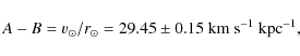
where the experimental values have been taken from Kerr & Lynden-Bell (1986). One observes that
The combination A-B can
be more precisely determined than the individual constants.
Kerr & Lynden-Bell (1986)
found ![]() km s-1 kpc-1.
km s-1 kpc-1.
Using the proper motion of the black hole in the Galactic
centre (Sgr A*) Reid &
Brunthaler (2004) found
in excellent agreement with recent measurements of parallaxes using the Very Large Baseline Interferometry (VLBI) (Reid et al. 2009), which yield
|
(11) |
From the velocities of stars orbiting Sgr A*, which is considered to be the centre of the Galaxy because of its small own velocity, the distance between the Sun and the GC has been determined to (Gillessen et al. 2009):
in agreement with previous authors (Ghez et al. 2008). With this Galactocentric distance one finds from Eq. (10) a rotation velocity of the Sun
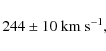
which is consistent with recent observations of Galactic masers in Bovy et al. (2009), who used data from the Very Long Baseline Array (VLBA) and the Japanese VLBI Exploration of Radio Astronomy (VERA). This speed determines the mass of the Galaxy inside the solar radius.
In this analysis two different rotation velocities are considered: the RC within the Galactic disc (Fig. 3) and the velocity distribution for stars outside the disc with z > 4 kpc (Fig. 4). They are discussed separately.
3.2.1 Rotation curve in the disc
For the RC within the disc a combination
of different measurements with different tracers has been summarized by
Sofue et al. (2008).
The experimental data, which can be found on the author's web page,
were scaled to ![]() km s-1
at a Galactocentric distance
of 8.3 kpc. Furthermore, the rotation velocity was averaged
in 17 radial bins from the GC to a radius of 22 kpc, as shown
in Fig. 3b
and tabulated in Table 2. The shape
of the measured
velocity distribution shows a strong increase of the rotation
velocity in the inner part of the Galaxy which presumably
results from the dense core of the Galaxy. For the inner Galaxy
the rotation curve is dominated by the visible matter and the
parametrization of Sect. 2.1 yields
a
reasonable description. However, at the outer Galaxy the experimental
data
cannot be explained: all profiles predict a slow decrease of
the rotation velocity in contrast to the data, which show first
a decrease between 6 and 10 kpc and then increases again.
Such a peculiar change of slope cannot be explained by a
smoothly decreasing DM density profile, but needs substructure,
e.g. the infall of a dwarf Galaxy, as mentioned in the
introduction and de Boer
et al. (2005). Such a ringlike
substructure is supported by the gas flaring
(Kalberla et al. 2007).
The thickness of the substructure is
of the order of 1 kpc, so it should not show up for halo stars
well above this height; this is indeed the case, as shown in
Fig. 4,
which will be discussed in the next
section.
km s-1
at a Galactocentric distance
of 8.3 kpc. Furthermore, the rotation velocity was averaged
in 17 radial bins from the GC to a radius of 22 kpc, as shown
in Fig. 3b
and tabulated in Table 2. The shape
of the measured
velocity distribution shows a strong increase of the rotation
velocity in the inner part of the Galaxy which presumably
results from the dense core of the Galaxy. For the inner Galaxy
the rotation curve is dominated by the visible matter and the
parametrization of Sect. 2.1 yields
a
reasonable description. However, at the outer Galaxy the experimental
data
cannot be explained: all profiles predict a slow decrease of
the rotation velocity in contrast to the data, which show first
a decrease between 6 and 10 kpc and then increases again.
Such a peculiar change of slope cannot be explained by a
smoothly decreasing DM density profile, but needs substructure,
e.g. the infall of a dwarf Galaxy, as mentioned in the
introduction and de Boer
et al. (2005). Such a ringlike
substructure is supported by the gas flaring
(Kalberla et al. 2007).
The thickness of the substructure is
of the order of 1 kpc, so it should not show up for halo stars
well above this height; this is indeed the case, as shown in
Fig. 4,
which will be discussed in the next
section.
Table 2: Averaged values of the Galactocentric distance and the rotation velocity shown in Fig. 3.
One may argue about the large uncertainties in the outer
rotation curve,
where the distance and the velocity have to be
determined
in contrast to the inner rotation curve, where the tangent
method yields the distance from the maximum velocity
(Binney 1998). The rotation
curve can be flattened, e.g. by
decreasing the distance between the Sun and the GC, but then
![]() kpc is needed (Honma & Sofue 1997),
which
is clearly outside the present errors given in Eq. (12).
Also the peculiar change of slope near 10 kpc does not
disappear. It should be noted that such a change of slope happens in
other spiral galaxies as well, as can be seen from the compilation of
rotation curves in Fig. 4 in Sofue & Rubin (2001).
For the smooth DM density profiles discussed in
this paper this feature will be neglected.
kpc is needed (Honma & Sofue 1997),
which
is clearly outside the present errors given in Eq. (12).
Also the peculiar change of slope near 10 kpc does not
disappear. It should be noted that such a change of slope happens in
other spiral galaxies as well, as can be seen from the compilation of
rotation curves in Fig. 4 in Sofue & Rubin (2001).
For the smooth DM density profiles discussed in
this paper this feature will be neglected.
3.2.2 Rotation curve in the halo
The data in Fig. 4
were obtained from a large
sample of roughly 2400 BHB stars,
as detected in the SDSS, with
Galactocentric distances up to about 60 kpc and vertical
heights of z > 4 kpc. In order to connect
the observable
values - line-of-sight velocity and distance - to the circular
velocity ![]() the halo
star distribution function from N-body simulations
of the Galaxy
with an NFW profile was used.
the halo
star distribution function from N-body simulations
of the Galaxy
with an NFW profile was used.
In order to compare our DM density profiles with these data,
the velocity curve is calculated for different angles with respect to
the Galactic disc.
Then the results are averaged. In Fig. 4
the averaged circular velocity curve and the velocity curves
for an inclination angle with the normal to the disc of 10![]() ,
45
,
45![]() and 80
and 80![]() are shown for the NFW profile. The averaged
circular velocity curves for the five other spherical halo profiles
discussed before are shown in
Fig. 4b.
The circular velocity distribution is consistent
with the cuspy halo profiles and the PISO profile. The 240 profile
cannot
describe the velocity distribution at large radii because of the too
steep
decrease of the density at large radii (
are shown for the NFW profile. The averaged
circular velocity curves for the five other spherical halo profiles
discussed before are shown in
Fig. 4b.
The circular velocity distribution is consistent
with the cuspy halo profiles and the PISO profile. The 240 profile
cannot
describe the velocity distribution at large radii because of the too
steep
decrease of the density at large radii (![]() 1/r4).
1/r4).
3.3 Surface density and Oort limit
Jan Oort proposed and performed another interesting measurement:
from the star count as function of their height above the disc
one obtains the local gravitational potential, which is directly
proportional to the mass in the plane of the MW.
Using the precise measurements from the Hipparcos satellite
Holmberg & Flynn (2004)
find for the local mass density, which
includes visible and dark matter,
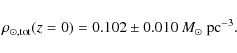
This value was determined by the precise star counts and velocity measurements in a volume of 125 pc around the Sun by the Hipparcos satellite. Korchagin et al. (2003) analysed the vertical potential at slightly larger distances (a vertical cylinder of 200 pc radius and an extension of 400 pc out of the Galactic plane). For the dynamical estimate of the local volume density they obtain the same value with a smaller error:
Integrating the density along the vertical direction
within ![]() z
from the Galactic plane yields the surface density:
z
from the Galactic plane yields the surface density:
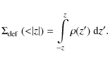
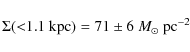
It can be calculated either by integrating the matter density distribution directly or by using the gravitational potential of the Galaxy. The integration limit is conventionally defined to be 1.1 kpc.
According to Eq. (7) this
definition is equal to
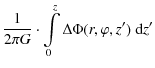
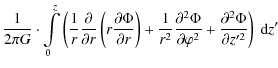
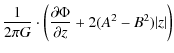

where A and B are the Oort constants discussed before. Since they are of the same order of magnitude, the surface density integrated to z is proportional to the derivative of the potential at height z, as shown by the last approximation in Eq. (16).
Table 3:
Contributions to the local surface density of baryonic matter. The
total values in the last row include ![]() errors.
errors.
![\begin{figure}
\par\includegraphics[width=9cm,angle=0,clip]{13381fg7.eps}
\end{figure}](/articles/aa/full_html/2010/01/aa13381-09/img104.png)
|
Figure 5:
The vertical gravitational potential at the position of the Sun |
| Open with DEXTER | |
Table 4:
Free and fixed parameters for the mass model of the Galaxy and
experimental constraints. One observes that there are 5 free parameters
and 8 constraints. Mass densities are in GeV cm-3
or in ![]() pc-3,
where
pc-3,
where ![]() cm
cm
![]() GeV cm-3.
GeV cm-3.
Table 5:
Fit results. The units of the different values are given in
Table 4.
The ![]() contributions are given below the variable value in brackets.
contributions are given below the variable value in brackets.
First the surface density of the luminous matter is
considered.
Its experimental value is determined by the summation of the
different contributions to the luminous matter -
the stellar population, stellar remnants and the interstellar gas.
A summary of the different measurements was given by Naab & Ostriker (2006).
The surface density of the baryonic matter lies between 35 and 58 ![]() pc-2
(Table 3),
which agrees with 48
pc-2
(Table 3),
which agrees with 48 ![]() 9
9
![]() pc-2
as estimated in Kuijken
& Gilmore (1991)
and Holmberg & Flynn
(2004).
pc-2
as estimated in Kuijken
& Gilmore (1991)
and Holmberg & Flynn
(2004).
Unfortunately, our local neighbourhood is not representative for the disc, since we live in a local underdensity - the local bubble - with an extension of a few hundred pc, which could have been caused by a series of rather recent SN explosions (Maiz-Apellaniz 2001). Therefore, a fit for the parameters of a mass model of the Galaxy might have a somewhat higher surface density than the locally observed value.
The total surface density at the position of the Sun was
determined by Kuijken &
Gilmore (1991) to be
from a parametrization of a mass distribution. In the paper by Holmberg & Flynn (2004) the modeling of the vertical gravitational potential resulted in
4 Numerical determination of the mass model of the Galaxy
![\begin{figure}
\par\includegraphics[width=14cm,angle=0,clip]{13381fg8.eps}
\end{figure}](/articles/aa/full_html/2010/01/aa13381-09/img131.png)
|
Figure 6:
The local DM densities |
| Open with DEXTER | |
As mentioned before, the three most important constraints for
the mass model of the Galaxy are given by the rotation curve
and the value ![]() ,
the total mass
,
the total mass ![]() and the local
mass density
and the local
mass density ![]() .
This can be easily seen as
follows:
.
This can be easily seen as
follows: ![]() ,
where
,
where ![]() and
and ![]() are proportional to
are proportional to ![]() and
and ![]() ,
respectively; for a given halo profile
,
respectively; for a given halo profile ![]() is determined
by
is determined
by ![]() ,
while the Oort limit
,
while the Oort limit ![]() determines
determines
![]() .
So in principle one has
3 constraints with only 2 variables
.
So in principle one has
3 constraints with only 2 variables ![]() and
and
![]() ,
if the shapes of the DM halo and the
visible matter would be known.
,
if the shapes of the DM halo and the
visible matter would be known.
Unfortunately, additional important parameters are i) the
eccentricity of the DM halo ii) the concentration of the DM
halo iii) the scale length of the disc iv) the mass in the
bar/bulge. In addition the mass model is sensitive to the
geometry, i.e. the Galactocentric distance from the Sun
![]() and the halo
profile. Additional constraints come
from the surface density, but here the visible surface density
has a large uncertainty as discussed before. The parameters and
constraints have been summarized in Table 4. The
parametrization of the mass of the bulge was chosen to describe
the rotation curve at small radii, which works reasonably well,
as can be seen from Fig. 3. Given that
the mass model
is not very sensitive to this inner region, the parameters of
the bulge will not be varied anymore.
and the halo
profile. Additional constraints come
from the surface density, but here the visible surface density
has a large uncertainty as discussed before. The parameters and
constraints have been summarized in Table 4. The
parametrization of the mass of the bulge was chosen to describe
the rotation curve at small radii, which works reasonably well,
as can be seen from Fig. 3. Given that
the mass model
is not very sensitive to this inner region, the parameters of
the bulge will not be varied anymore.
To optimize the remaining parameters in order to best describe
the
data, the following ![]() function was minimized using the Minuit
package (James & Roos 1975)
function was minimized using the Minuit
package (James & Roos 1975)
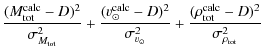
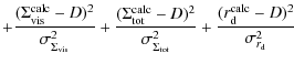
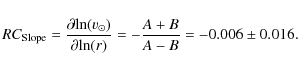
The index
The fit shows a more than 95% positive correlation between the
local dark matter density and the scale length of DM halo a
and an equally large negative correlation with the scale length
![]() of the
baryonic disc. Consequently, it is difficult to
leave parameters free in the fit. Therefore the fit was
first performed for fixed values of a (rows 1-3 of Table 5)
and then
of the
baryonic disc. Consequently, it is difficult to
leave parameters free in the fit. Therefore the fit was
first performed for fixed values of a (rows 1-3 of Table 5)
and then ![]() was fixed (rows 4-7). With the other free parameters all experimental
constraints could be met, as indicated by the
was fixed (rows 4-7). With the other free parameters all experimental
constraints could be met, as indicated by the ![]() values
in brackets below the fitted values in Table 5. Of
course, the total mass changed for the different fits. Figure 6 shows
the resulting local DM density versus the total mass, as calculated
from the fitted parameters. It shows that in spite of the small errors
for the local density in
individual fits the spread in density is still quite large.
values
in brackets below the fitted values in Table 5. Of
course, the total mass changed for the different fits. Figure 6 shows
the resulting local DM density versus the total mass, as calculated
from the fitted parameters. It shows that in spite of the small errors
for the local density in
individual fits the spread in density is still quite large.
The fit was repeated for other halo profiles, which gave
similarly good ![]() values, as shown by rows 9-11 in Table 5. So with the
present data one cannot distinguish
the different halo profiles.
values, as shown by rows 9-11 in Table 5. So with the
present data one cannot distinguish
the different halo profiles.
Sofar only spherical haloes have been discussed. Allowing
oblate
haloes with a ratio of short-to-long axis of 0.7 the local DM
density increases by about 20%, as shown by the last row of
Table 5.
As mentioned before, dark discs can
enhance this value considerably more, so the uncertainty
usually quoted for the local dark matter density in the range
of 0.2 to 0.7 GeV cm-3
(0.005-0.018 ![]() pc-3)
(Gates
et al. 1995; Amsler et al. 2008)
is still valid
in spite of the considerably improved data.
pc-3)
(Gates
et al. 1995; Amsler et al. 2008)
is still valid
in spite of the considerably improved data.
5 Conclusion
In this analysis five different halo profiles are compared with recent dynamical constraints as summarized in Table 4. The change of slope in the RC around 10 kpc (Fig. 3) was ignored, so the monotonical decreasing RC for the smooth halo profiles do not describe the data well. The change of slope may be related to a ringlike DM substructure, as indicated by the structure in the gas flaring (Kalberla et al. 2007) and by the structure in the diffuse gamma radiation (de Boer et al. 2005). Such a ringlike structure of DM gives a perfect description of the rotation curve, especially the fast decrease between 6 and 10 kpc. If the DM substructure is included, the local DM density increases above the values found in this analysis, so the values quoted here should be considered lower limits.
The astronomical constraints are
consistent with a density model of the Galaxy consisting of a
central bulge, a disc and an extended DM halo with a cuspy
density profile and a local DM density between 0.2 GeV
cm-3 (0.005 ![]() pc-3)
and 0.4 GeV cm-3 (0.01
pc-3)
and 0.4 GeV cm-3 (0.01 ![]() pc-3),
as shown in Fig. 6.
Strong positive and negative correlations between the parameters were
found in the fit
and they are causing the obvious correlations between
pc-3),
as shown in Fig. 6.
Strong positive and negative correlations between the parameters were
found in the fit
and they are causing the obvious correlations between
![]() and
and ![]() in Fig. 6.
For non-spherical haloes these values can be enhanced by
20%. If dark discs are considered, densities up to
0.7 GeV cm-3 (0.018
in Fig. 6.
For non-spherical haloes these values can be enhanced by
20%. If dark discs are considered, densities up to
0.7 GeV cm-3 (0.018 ![]() pc-3)
can be easily imagined, so the previous quoted range of
0.2-0.7 GeV cm-3
(0.005-0.018
pc-3)
can be easily imagined, so the previous quoted range of
0.2-0.7 GeV cm-3
(0.005-0.018 ![]() pc-3)
seems still valid. This range is considerably larger than the values
quoted by
analyses which used a Markov Chain method to minimize the
likelihood; they find
pc-3)
seems still valid. This range is considerably larger than the values
quoted by
analyses which used a Markov Chain method to minimize the
likelihood; they find ![]() GeV cm-3
(Catena & Ullio 2009)
and
GeV cm-3
(Catena & Ullio 2009)
and ![]() GeV cm-3
(Strigari & Trotta 2009)
respectively.
But given the good
GeV cm-3
(Strigari & Trotta 2009)
respectively.
But given the good ![]() values for our fits obtained for a large range of DM densities we see
no way that the errors can be as small as quoted by these authors.
values for our fits obtained for a large range of DM densities we see
no way that the errors can be as small as quoted by these authors.
References
- Amsler, C., Doser, M., Antonelli, M., et al. 2008, Phys. Lett., B 667, 1 [Google Scholar]
- Battaglia, G., Helmi, A., Morrsion, H., et al. 2005, MNRAS, 364, 433 [NASA ADS] [CrossRef] [Google Scholar]
- Battaglia, G., Helmi, A., Morrsion, H., et al. 2006, MNRAS, 370, 1055 [NASA ADS] [CrossRef] [Google Scholar]
- Bekenstein, J., & Milgrom, M. 1984, AJ, 286, 7 [NASA ADS] [CrossRef] [Google Scholar]
- Bienayme, O., Soubiran, C., Mishenina, T. V., Kovtyukh, V. V., & Siebert, A. 2005, A&A, 446, 933 [Google Scholar]
- Bienayme, O., Famaey, B., Wu, X., Zhao, H. S., & Aubert, D. 2009, A&A, 500, 801 [Google Scholar]
- Binney, J. J., & Evans, N. W. 2001, MNRAS, 327, L27 [NASA ADS] [CrossRef] [Google Scholar]
- Binney, E., & Merrifield, M. R. 1998, Galactic astronomy (Princeton University Press) [Google Scholar]
- Blumenthal, G. R., Faber, S. M., Flores, R., & Primack, J. R. 1986, ApJ, 301, 27 [NASA ADS] [CrossRef] [MathSciNet] [Google Scholar]
- Bovy, J., Hogg, D. W., & Rix, H.-W. 2009, ApJ, 704, 1704 [NASA ADS] [CrossRef] [Google Scholar]
- Cardone, V. F., & Sereno, M. 2005, A&A, 438, 545 [Google Scholar]
- Catena, R., & Ullio, P. 2009, JCAP, submitted [Google Scholar]
- Dame, T. M. 1993, in Back to the Galaxy, ed. S. S. Holt, & F. Verter, AIP Conf., 278, 267 [Google Scholar]
- de Boer, W., Sander, C., Zhukov, V., Gladyshev, A. V., & Kazakov, D. I. 2005, A&A, 444, 51 [Google Scholar]
- Freudenreich, H. T. 1998, ApJ, 492, 495 [NASA ADS] [CrossRef] [Google Scholar]
- Fuchs, B., Dettbarn, C., Rix, H.-W., et al. 2009, AJ, 137, 4149 [NASA ADS] [CrossRef] [Google Scholar]
- Gates, E. I., Gyuk, G., & Turner, M. S. 1995, ApJ, 449, L123 [Google Scholar]
- Gentile, G., Tonini, C., & Salucci, P. 2007, A&A, 467, 925 [Google Scholar]
- Ghez, A. M., Salim, S., Weinberg, N. N., et al. 2008, ApJ, 689, 1044 [NASA ADS] [CrossRef] [Google Scholar]
- Gillessen, S., Eisenhauer, F., Trippe, S., et al. 2009, ApJ, 692, 1075 [NASA ADS] [CrossRef] [Google Scholar]
- Gilmore, G., & Reid, N. 1983, MNRAS, 202, 1025 [NASA ADS] [CrossRef] [Google Scholar]
- Gilmore, G., Wyse, R. F. G., & Kuijken, K. 1989, in Evolutionary phenomena in galaxies (Cambridge University Press), 172 [Google Scholar]
- Gould, A., Bahcall, J. N., & Flynn, C. 1996, ApJ, 465, 759 [NASA ADS] [CrossRef] [Google Scholar]
- Gunn, J. E. 1977, ApJ, 218, 592 [NASA ADS] [CrossRef] [Google Scholar]
- Hammer, F., Puech, M., Chemin, L., Flores, H., & Lehnert, M. 2007, ApJ, 662, 322 [NASA ADS] [CrossRef] [Google Scholar]
- Holmberg, J., & Flynn, C. 2004, MNRAS, 352, 440 [NASA ADS] [CrossRef] [Google Scholar]
- Honma, M., & Sofue, Y. 1997, Astron. Soc. Japan, 48, L103 [Google Scholar]
- James, F., & Roos, M. 1975, Comput. Phys. Commun., 10, 343 [NASA ADS] [CrossRef] [PubMed] [Google Scholar]
- Kalberla, P. M. W., Dedes, L., Kerp, J., & Haud, U. 2007, A&A, 469, 511 [Google Scholar]
- Kerr, F. J., & Lynden-Bell, D. 1986, MNRAS, 221, 1023 [NASA ADS] [CrossRef] [Google Scholar]
- Klypin, A., Zhao, H., & Somerville, R. S. 2002, ApJ, 573, 597 [Google Scholar]
- Korchagin, V. I., Girard, T. M., Borkova, T. V., Dinescu, D. I., & van Altena, W. F. 2003, AJ, 126, 2869 [Google Scholar]
- Kroupa, P., Tout, C. A., & Gilmore, G. 1993, MNRAS, 262, 545 [NASA ADS] [CrossRef] [Google Scholar]
- Kuijken, K., & Gilmore, G. 1991, ApJ, 367, L9 [NASA ADS] [CrossRef] [Google Scholar]
- Ludlow, A. D., Navarro, J. F., Springel, V., et al. 2009, ApJ, 692, 931 [NASA ADS] [CrossRef] [Google Scholar]
- Maiz-Apellaniz, J. 2001, ApJ, 560, L83 [NASA ADS] [CrossRef] [Google Scholar]
- Mashchenko, S., Couchman, H. M. P., & Wadsley, J. 2006, Nature, 442, 539 [NASA ADS] [CrossRef] [PubMed] [Google Scholar]
- Mera, D., Chabrier, G., & Schaeffer, R. 1998, A&A, 330, 937 [Google Scholar]
- Merrifield, M. R. 1992, AJ, 103, cITA-91-44 [PubMed] [Google Scholar]
- Moore, B., Ghigna, S., Governato, F., et al. 1999, ApJ, 524, L19 [Google Scholar]
- Naab, T., & Ostriker, J. P. 2006, MNRAS, 366, 899 [NASA ADS] [CrossRef] [Google Scholar]
- Navarro, J. F., Frenk, C. S., & White, S. D. M. 1997, ApJ, 490, 493 [NASA ADS] [CrossRef] [Google Scholar]
- Oh, S.-H., de Blok, W. J. G., Walter, F., Brinks, E., & Kennicutt, Robert C. J. 2008, AJ, 136, 2761 [NASA ADS] [CrossRef] [Google Scholar]
- Ojha, D., Bienayme, O., Robin, A., Creze, M., & Mohan, V. 1996, A&A, 311, 456 [Google Scholar]
- Olling, R. P., & Merrifield, M. R. 2001, MNRAS, 326, 164 [NASA ADS] [CrossRef] [Google Scholar]
- Purcell, C. W., Bullock, J. S., & Kaplinghat, M. 2009, ApJ, 703, 2275 [NASA ADS] [CrossRef] [Google Scholar]
- Reid, M. J. 2009, Int. J. Mod. Phys., D18, 889 [Google Scholar]
- Reid, M. J., & Brunthaler, A. 2004, ApJ, 616, 872 [NASA ADS] [CrossRef] [Google Scholar]
- Reid, M. J., Menten, K. M., Zheng, X. W., et al. 2009, ApJ, 700, 137 [NASA ADS] [CrossRef] [Google Scholar]
- Ricotti, M. 2003, MNRAS, 344, 1237 [NASA ADS] [CrossRef] [Google Scholar]
- Robin, A. C., Haywood, M., Creze, M., Ojha, D. K., & Bienayme, O. 1996, A&A, 305, 125 [Google Scholar]
- Sakamoto, T., Chiba, M., & Beers, T. C. 2003, A&A, 397, 899 [Google Scholar]
- Salucci, P. et al. 2007, MNRAS., 378, 41 [NASA ADS] [CrossRef] [Google Scholar]
- Sofue, Y., & Rubin, V. 2001, ARA&A, 39, 137 [Google Scholar]
- Sofue, Y., Honma, M., & Omodaka, T. 2008, Astron. Soc. Japan, 61, 227 [Google Scholar]
- Sparke, L. S., & Gallagher, J. S. 2007, Galaxies in the Universe - An Introduction (Cambridge University Press) [Google Scholar]
- Spooner, N. J. 2007, J. Phys. Soc. Jap., 76, 111016 [NASA ADS] [CrossRef] [Google Scholar]
- Springel, V., White, S. D. M., Frenk, C. S., et al. 2008a [arXiv:0809.0894] [Google Scholar]
- Springel, W., S. D. M., Frenk, C. S., et al. 2008b, Nature, 456, 73 [NASA ADS] [CrossRef] [PubMed] [Google Scholar]
- Strigari, L. E., & Trotta, R. 2009, JCAP, in press [Google Scholar]
- Wilkinson, M. I., & Evans, N. W. 1999, MNRAS, 310, 645 [NASA ADS] [CrossRef] [Google Scholar]
- Xue, X. X., Rix, H. W., Zhao, G., et al. 2008, ApJ, 684, 1143 [NASA ADS] [CrossRef] [Google Scholar]
- Zeilik, M., & Gregory, S. 1998, Introductory Astronomy and Astrophysics (Saunders College) [Google Scholar]
- Zheng, Z., Flynn, C., Gould, A., Bahcall, J. N., & Salim, S. 2001, ApJ, 555, 393 [NASA ADS] [CrossRef] [Google Scholar]
All Tables
Table 1: Parameter settings for the different DM halo profiles considered in this analysis.
Table 2: Averaged values of the Galactocentric distance and the rotation velocity shown in Fig. 3.
Table 3:
Contributions to the local surface density of baryonic matter. The
total values in the last row include ![]() errors.
errors.
Table 4:
Free and fixed parameters for the mass model of the Galaxy and
experimental constraints. One observes that there are 5 free parameters
and 8 constraints. Mass densities are in GeV cm-3
or in ![]() pc-3,
where
pc-3,
where ![]() cm
cm
![]() GeV cm-3.
GeV cm-3.
Table 5:
Fit results. The units of the different values are given in
Table 4.
The ![]() contributions are given below the variable value in brackets.
contributions are given below the variable value in brackets.
All Figures
|
|
Figure 1:
Radial DM density distribution for the parameters given in
Table 1.
The normalization |
| Open with DEXTER | |
| In the text | |
|
|
Figure 2:
The mass inside a radius as function of that radius is shown for the
different halo profiles defined in Table 1. The thin
solid line represents the visible mass which is different for different
halo profiles because of the variation of the parameters |
| Open with DEXTER | |
| In the text | |
|
|
Figure 3: The rotation curves - calculated for different halo profiles - in comparison with experimental data, which have been adapted from the publication by Sofue et al. (2008). On the left side all data points are shown, while on the right side a weighted average of the experimental data is shown in 17 radial bins. |
| Open with DEXTER | |
| In the text | |
|
|
Figure 4: The circular velocity curve for halo stars above a height of z > 4 kpc is shown. On the left side the circular velocity curve for the NFW profile calculated for different angles with respect to the Galactic disc is shown. On the right side the averaged circular velocity curves for the different halo profiles are shown. The experimental data were obtained from the publication by Xue et al. (2008). |
| Open with DEXTER | |
| In the text | |
|
|
Figure 5:
The vertical gravitational potential at the position of the Sun |
| Open with DEXTER | |
| In the text | |
|
|
Figure 6:
The local DM densities |
| Open with DEXTER | |
| In the text | |
Copyright ESO 2010
Current usage metrics show cumulative count of Article Views (full-text article views including HTML views, PDF and ePub downloads, according to the available data) and Abstracts Views on Vision4Press platform.
Data correspond to usage on the plateform after 2015. The current usage metrics is available 48-96 hours after online publication and is updated daily on week days.
Initial download of the metrics may take a while.