| Issue |
A&A
Volume 509, January 2010
|
|
|---|---|---|
| Article Number | A82 | |
| Number of page(s) | 9 | |
| Section | Cosmology (including clusters of galaxies) | |
| DOI | https://doi.org/10.1051/0004-6361/200912525 | |
| Published online | 22 January 2010 | |
Galaxy clusters as mirrors of the distant Universe
Implications of the blurring term for the kSZ and ISW effects
C. Hernández-Monteagudo1 - R. A. Sunyaev1,2
1 - Max-Planck-Institut für Astrophysik, Karl-Schwarzschild-Str. 1, 85741
Garching bei München, Germany
2 -
Space Research Institute, Russian Academy of Sciences, Profsoyuznaya 84/32, 117997 Moscow, Russia
Received 19 May 2009 / Accepted 26 October 2009
Abstract
It is well known that Thomson scattering of cosmic microwave
background (CMB) photons in galaxy clusters introduces new anisotropies
in the CMB radiation field, but still little attention is payed to
the fraction of CMB photons that are scattered off the line of sight, causing a slight blurring of the CMB anisotropies present at the moment of scattering. In this work we study this blurring
effect and find that it can provide an independent measurement of the
cluster's gas mass. Likewise, this effect has a non-negligible impact
on estimations of the
kSZ effect: it induces a 10% correction in 20-40%
of the clusters/groups and a dominant over kSZ correction in ![]() %
of the clusters in an ideal (noiseless) experiment. For rich clusters,
CMB, tSZ and X-ray observations can provide estimates for the amplitude
and sign of the blurring effect that can be used for correcting
kSZ estimations. We explore the possibility of using this blurring
term to probe the CMB anisotropy field at different epochs in our
Universe. In particular, we study the required precision in the
removal of the kSZ which enables us to detect the blurring
term
%
of the clusters in an ideal (noiseless) experiment. For rich clusters,
CMB, tSZ and X-ray observations can provide estimates for the amplitude
and sign of the blurring effect that can be used for correcting
kSZ estimations. We explore the possibility of using this blurring
term to probe the CMB anisotropy field at different epochs in our
Universe. In particular, we study the required precision in the
removal of the kSZ which enables us to detect the blurring
term
![]() in
galaxy cluster populations placed at different redshift shells.
By mapping this term in those shells, we provide a tomographic
probe for the growth of the Integrated Sachs-Wolfe effect (ISW) during
the late evolutionary stages of the Universe. We find that the required
precision on the removal of the cluster's peculiar velocity is of the
order of 100-200 km s-1 in the redshift range 0.2-0.8, after assuming that all clusters more massive than 10
in
galaxy cluster populations placed at different redshift shells.
By mapping this term in those shells, we provide a tomographic
probe for the growth of the Integrated Sachs-Wolfe effect (ISW) during
the late evolutionary stages of the Universe. We find that the required
precision on the removal of the cluster's peculiar velocity is of the
order of 100-200 km s-1 in the redshift range 0.2-0.8, after assuming that all clusters more massive than 10
![]() are observable. These errors are comparable to the total expected
linear line of sight velocity dispersion for clusters in
WMAPV cosmogony and correspond to a residual level of roughly
900-1800
are observable. These errors are comparable to the total expected
linear line of sight velocity dispersion for clusters in
WMAPV cosmogony and correspond to a residual level of roughly
900-1800
![]() K
per cluster, including all types of contaminants and systematics. Were
this precision requirement achieved, then independent constraints on
the intrinsic cosmological dipole would be simultaneously provided.
K
per cluster, including all types of contaminants and systematics. Were
this precision requirement achieved, then independent constraints on
the intrinsic cosmological dipole would be simultaneously provided.
Key words: cosmic microwave background - large-scale structure of Universe
1 Introduction
The study of the scattering of cosmic microwave background (CMB) photons in moving clouds of thermal electrons (like galaxy clusters) has been a subject of active research since the first works of Sunyaev & Zeldovich (1980,1972); Zeldovich & Syunyaev (1980); Sunyaev & Zeldovich (1970,1981). Indeed, this mechanism is one of the key two sources for intensity and polarization anisotropies in the CMB (the other one being associated to the presence of gravitational fields, the so-called Sachs-Wolfe effect, Sachs & Wolfe 1967). The Thomson scattering changes the angular distribution of the CMB photons, partially erasing the original anisotropy pattern (due to the off scattering of photons propagating initially along the line of sight) and introducing new anisotropies if the electrons move with respect to the CMB rest frame. Due to its anisotropic nature, Thomson scattering also introduces linear polarization if the CMB shows an intensity quadrupole at the scattering place. The use of the polarization induced by Thomson scattering in galaxy clusters has been proposed as a probe for remote CMB quadrupoles (Kamionkowski & Loeb 1997; Challinor et al. 2000; Sunyaev & Zeldovich 1980; Sazonov & Sunyaev 1999), with implications for the integrated Sachs-Wolfe effect (ISW, Cooray & Baumann 2003) and for the characterization of the large scale density distribution in the observable universe (e.g., Abramo & Xavier 2007; Seto & Sasaki 2000).
However, this work will be devoted to the study of a blurring
term, i.e., the term responsible for the smearing of the intensity
anisotropies of the radiation field generated early enough, either at
recombination or during reionization, or before the phase of
accelerated expansion of the universe. For an axisymmetric radiation
field described by
![]() (with
(with
![]() measuring deviations from the symmetry axis), the blurring term will affect all multipoles, whereas the anisotropic scattering will slightly modify the quadrupole (a2) and generate a secondary polarization (e.g. Sunyaev & Zeldovich 1980; Zeldovich & Syunyaev 1980; Sunyaev & Zeldovich 1981):
measuring deviations from the symmetry axis), the blurring term will affect all multipoles, whereas the anisotropic scattering will slightly modify the quadrupole (a2) and generate a secondary polarization (e.g. Sunyaev & Zeldovich 1980; Zeldovich & Syunyaev 1980; Sunyaev & Zeldovich 1981):
where al=1 refers to the intrinsic cosmological dipole at the scattering place. This dipole must not be confused with the dipole observed by COBE and WMAP, which is mainly caused by the observer's local peculiar motion. The blurring term is described by the right hand side of the equation above (note that the quadrupole is effectively suppressed by a factor of only
with
If detected on a set of cluster samples placed at different redshifts, the bSZ term can be used as a probe in situ of the CMB anisotropy field at those epochs. By looking at the variations of this term in different redshift shells, one should be able to track the growth of new anisotropies arising at later times. In particular, it should enable us to perform tomography of the ISW effect, generated by the decay of the linear gravitational potentials at late epochs.
This acquires particular relevance in the context of current SZ cluster surveys like SPT (Staniszewski et al. 2009), ACT (Hincks et al. 2009) or Planck, and future surveys like the X-ray mission SPECTRUM-X/eROSITA![]() , whose prospect is to locate
, whose prospect is to locate
![]() galaxy clusters in the sky (among them all clusters above 2
galaxy clusters in the sky (among them all clusters above 2 ![]()
![]() in
the observable Universe). Some of these clusters will sit on top of
high amplitude CMB intensity excursions where this effect can be
measured more easily. Furthermore, we also show that this
phenomenon should also provide stringent limits on the amplitude of the
intrinsic cosmological dipole.
in
the observable Universe). Some of these clusters will sit on top of
high amplitude CMB intensity excursions where this effect can be
measured more easily. Furthermore, we also show that this
phenomenon should also provide stringent limits on the amplitude of the
intrinsic cosmological dipole.
This paper is organized as follows: in Sect. 2 we describe the blurring term within the context of Thomson scattering. In Sect. 3 we study its implications in the measurement of kSZ and remote quadrupoles at the position of galaxy clusters. In Sect. 4 we introduce the possibility of using the blurring term for tracking the growth of the ISW: we analyse the requirements in the cluster sample and in the peculiar velocity recovery. We observe the possibility of setting constraints on the cosmological dipole by using this effect in Sect. 5. Finally, in Sect. 6 we discuss our results and conclude.
2 The scattering of CMB photons in electron clouds
Thomson scattering modifies the angular pattern of the CMB intensity and polarization anisotropies. The source for new intensity anisotropies is associated with the peculiar velocity of the gas cloud with respect to the CMB frame (Sunyaev & Zeldovich 1980), whereas in the case of polarization anisotropies it is associated with the CMB quadrupole at the scattering place. If the electron gas is at a high temperature, then Compton scattering transfers energy from the electron plasma to the CMB photon field, distorting the CMB black body spectrum and introducing frequency dependent temperature fluctuations (tSZ effect). The tSZ effect (and its relativistic corrections) has a definite spectral dependence (Sunyaev & Zeldovich 1972; Itoh & Nozawa 2004; Rephaeli 1995; Sunyaev & Zeldovich 1981), so hereafter we shall assume that it can be accurately subtracted.
Our interest in this paper will be focused on the intensity blurring term (
![]() ), which accounts for the fraction of photons that, initially propagating along the line of sight, were scattered off it and never reach the observer. This term hence describes the erasing of the CMB anisotropies at the scattering position along the line of sight towards the electron cloud, since the Thomson scattering tends to isotropize
the CMB angular fluctuations in that direction. This adds up to
the kSZ effect, with no distinction on the photon's frequency and
hence preserving the CMB black body spectrum. The source of the
polarization, instead, is the cluster's local CMB intensity quadrupole, which is sensitive to the CMB at all
directions in that position. In the following considerations we regard
the galaxy cluster and group population as clouds of free electrons.
), which accounts for the fraction of photons that, initially propagating along the line of sight, were scattered off it and never reach the observer. This term hence describes the erasing of the CMB anisotropies at the scattering position along the line of sight towards the electron cloud, since the Thomson scattering tends to isotropize
the CMB angular fluctuations in that direction. This adds up to
the kSZ effect, with no distinction on the photon's frequency and
hence preserving the CMB black body spectrum. The source of the
polarization, instead, is the cluster's local CMB intensity quadrupole, which is sensitive to the CMB at all
directions in that position. In the following considerations we regard
the galaxy cluster and group population as clouds of free electrons.
![\begin{figure}
\par\includegraphics[height=7.8cm,width=7.5cm,clip]{12525fg1.eps}
\end{figure}](/articles/aa/full_html/2010/01/aa12525-09/img27.png)
|
Figure 1:
Fraction of the total CMB temperature rms that corresponds to scales
larger than the cluster size. The change of slope at
|
| Open with DEXTER | |
![\begin{figure}
\par\includegraphics[height=13.3cm,width=7cm,clip]{12525fg2.eps}
\end{figure}](/articles/aa/full_html/2010/01/aa12525-09/img28.png)
|
Figure 2:
Top panel: total CMB map with two clusters for which the tSZ and the kSZ contributions have been removed. A high value of
|
| Open with DEXTER | |
2.1 Estimating the blurring effect
Both bSZ and kSZ have exactly the same spectral dependence, and this
complicates their separation. However, current and future
multifrequency CMB observations should provide estimates of the
tSZ at each cluster's position. Indeed, tSZ measurements are
currently being provided by experiments
like SPT, ACT, BIMA, CBI, SZA, AMI, or AMIBA in more than a hundred
galaxy clusters. By combining these measurements with X-ray
derived estimates of the gas temperature (![]() ,
provided by, e.g., CHANDRA or XMM) one can find the cluster's optical depth
,
provided by, e.g., CHANDRA or XMM) one can find the cluster's optical depth
![]() ,
,
where the function
with
When averaging over the cluster's area, it is relevant to know
the amplitude of the rms CMB fluctuations which is being blurred
by the cluster. This can be computed by simply adding up the
contribution of different angular scales or multipoles to the
CMB variance up to the cluster scale,
![\begin{displaymath}%
\sigma_{\rm CMB}^2 [l_{\rm cl}] = \sum_{l=1}^{l=l_{\rm cl}} \frac{2l+1}{4\pi} C_l,
\end{displaymath}](/articles/aa/full_html/2010/01/aa12525-09/img42.png)
where
2.2 Sensitivity to the total electron content of the cluster
The bSZ term can be used to measure the number of electrons present in
a galaxy cluster. It depends linearly on the Thomson optical
depth
![]() and
on the CMB temperature fluctuations at the place of scattering.
The latter should be accurately mapped by ongoing CMB experiments
like WMAP,
Planck, or, at higher angular resolution, by ACT or SPT. The
measurement of the bSZ at different projected distances to the
cluster's center would therefore provide a useful handle on the
electron content and, after assuming a baryon mass fraction (e.g. Giodini et al. 2009; Vikhlinin et al. 2006; Ettori et al. 2009),
on the entire mass profile of the cluster. This can easily been seen by
writing the baryonic mass profile of the cluster in terms of its
Thomson optical depth:
and
on the CMB temperature fluctuations at the place of scattering.
The latter should be accurately mapped by ongoing CMB experiments
like WMAP,
Planck, or, at higher angular resolution, by ACT or SPT. The
measurement of the bSZ at different projected distances to the
cluster's center would therefore provide a useful handle on the
electron content and, after assuming a baryon mass fraction (e.g. Giodini et al. 2009; Vikhlinin et al. 2006; Ettori et al. 2009),
on the entire mass profile of the cluster. This can easily been seen by
writing the baryonic mass profile of the cluster in terms of its
Thomson optical depth:
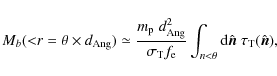
where
For the case of unresolved clusters, the bSZ would provide a measurement of the total baryon content of those objects directly. This constitutes a useful independent test for mass estimates in clusters of galaxies, which are of an utmost importance in cosmological studies of tSZ surveys.
3 Impact on kSZ estimations
Let us consider here the case where the peculiar velocity of the gas is
equal to that of dark matter. Let us keep in mind, however, that
bulk velocities of gas inside massive galaxy clusters may significantly
exceed the peculiar speed of the entire cluster (Sunyaev et al. 2003; Inogamov & Sunyaev 2003).
As mentioned above, the kSZ effect in clusters has the same
spectral dependence of the intrinsic CMB anisotropies, and
therefore extracting it requires the use of spatial frequency
information. Its amplitude is directly proportional to the
projection of the cluster's peculiar velocity along the line of sight.
In linear theory and after assuming that the initial rotational
component of the
peculiar velocity field is negligible (since it scales with the
inverse of the cosmological expansion scale factor), it is
possible to relate the Fourier modes of the peculiar velocity with
those of the matter density field (
![]() ):
):
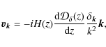
where H(z) is the Hubble function and
![\begin{displaymath}%
\sigma_v^2 (M)= \frac{1}{3} \int \frac{{\rm d}{\vec {k}}}{(...
...}\biggr\vert^2 \frac{P_{\rm m}(k)}{k^2} \vert W(kR[M])\vert^2,
\end{displaymath}](/articles/aa/full_html/2010/01/aa12525-09/img60.png)
where W(kR[M]) is the Fourier window function of a top hat filter of size given by the linear scale corresponding to the cluster mass M,
![\begin{figure}
\par\includegraphics[height=12.5cm,width=7.8cm,clip]{12525fg3.eps}
\vspace*{5mm}
\end{figure}](/articles/aa/full_html/2010/01/aa12525-09/img69.png)
|
Figure 3:
a) Amplitude of the linear rms radial peculiar velocity in a WMAPV cosmology for a 2 |
| Open with DEXTER | |
We have adopted an average bias of 30% in the halo peculiar velocities,
and estimated the average correction to the kSZ which the bSZ term
causes. We have assumed accordingly that both the CMB temperature
anisotropies and the kSZ fluctuations are Gaussian distributed and
computed the fraction of clusters whose kSZ undergoes a correction
above a certain level
![]() due to the bSZ effect:
due to the bSZ effect:
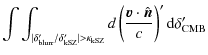
![$\displaystyle \times ~ p(\delta_{\rm CMB}')\; p\left[\left(\frac{{\vec {v}}\cdot\hat{{\vec {n}}}}{c}\right)' \right].$](/articles/aa/full_html/2010/01/aa12525-09/img73.png)
In both cases, the function p(X) denoted the Gaussian probability distribution function on the variable X. The term
4 Implications for the ISW effect
By measuring the intensity blurring term through the lines of sight
towards clusters placed at a given redshift shell an estimate of the
CMB temperature field at that redshift is obtained. In Fig. 4a
we show the CMB TT (intensity) power spectrum as measured by
observers placed at different redshifts; the thick solid line
corresponds to z=0, the dotted line to z=0.1, the dashed line to z=1 and the dot-dashed line to z=2.
Since those observers are closer to the surface of last scattering, the
whole acoustic pattern shifts to larger angular scales (smaller
multipoles). Furthermore, at redshifts larger than ![]() the contribution of the ISW is very small, and this is also visible in the low l
range. After the scattering, the angular pattern of the
CMB anisotropies would stream unhindered towards the observer,
shifting the whole picture ``back'' to its standard position,
(see Fig. 4b). In Fig. 5 we display the free streaming of the CMB quadrupole multipole
the contribution of the ISW is very small, and this is also visible in the low l
range. After the scattering, the angular pattern of the
CMB anisotropies would stream unhindered towards the observer,
shifting the whole picture ``back'' to its standard position,
(see Fig. 4b). In Fig. 5 we display the free streaming of the CMB quadrupole multipole
![]() as seen by an observer placed at different redshifts into different multipoles al,0-s. The case of redshift z=0.1 is displayed by solid circles joined by a solid black line, z=1 by red triangles joined by a dashed line, and z=2
by green squares joined by a dot-dashed line. The further away the
remote observer is, the more power is aliased into high l
multipoles. This streaming of the CMB angular anisotropies permits
us a comparison of the ISW pattern at different cosmological
epochs on the angular/multipole scale. If the bSZ term is observed
through the line of sights corresponding to a population of galaxy
clusters and groups situated at a high redshift, it would provide a
picture of the CMB pattern before the ISW arises.
This means that, by observing the bSZ term in galaxy clusters
placed at different redshift shells it should be possible, a priori, to
track the growth of the ISW effect with decreasing redshift.
as seen by an observer placed at different redshifts into different multipoles al,0-s. The case of redshift z=0.1 is displayed by solid circles joined by a solid black line, z=1 by red triangles joined by a dashed line, and z=2
by green squares joined by a dot-dashed line. The further away the
remote observer is, the more power is aliased into high l
multipoles. This streaming of the CMB angular anisotropies permits
us a comparison of the ISW pattern at different cosmological
epochs on the angular/multipole scale. If the bSZ term is observed
through the line of sights corresponding to a population of galaxy
clusters and groups situated at a high redshift, it would provide a
picture of the CMB pattern before the ISW arises.
This means that, by observing the bSZ term in galaxy clusters
placed at different redshift shells it should be possible, a priori, to
track the growth of the ISW effect with decreasing redshift.
![\begin{figure}
\par\includegraphics[height=10.8cm,width=8.8cm,clip]{12525fg4.eps}
\end{figure}](/articles/aa/full_html/2010/01/aa12525-09/img83.png)
|
Figure 4: a) CMB TT angular power spectrum as seen by observers placed at redshifts z=0, 0.1, 1 and 2 (solid, dotted, dashed and dot-dashed lines, respectively). b) Same power spectra as in a) after being free streamed to the present moment. |
| Open with DEXTER | |
![\begin{figure}
\par\includegraphics[height=7cm,width=8cm,clip]{12525fg5.eps}
\end{figure}](/articles/aa/full_html/2010/01/aa12525-09/img84.png)
|
Figure 5: Projection of the CMB quadrupole multipole a2,0 as seen by observers placed at different redshifts into different al,0 multipoles observed at present. Filled circles connected with a black solid line correspond to an observer placed at z=0.1, red triangles by a red dashed line to an observer at z=1 and green squares linked by a dot-dashed line to z=2. |
| Open with DEXTER | |
In the future, several surveys in the optical and in the X-ray range (Pan-STARRS![]() , DES
, DES![]() , PAU-BAO
, PAU-BAO![]() , Benitez et al. 2008, Spectrum-X/eROSITA) will probe the cosmological density field up to redshifts
, Benitez et al. 2008, Spectrum-X/eROSITA) will probe the cosmological density field up to redshifts
![]() with unprecedented sensitivity. Gravity relates the matter density
distribution with the peculiar motion it causes, so a good
estimation for the kSZ in clusters and groups should be obtainable from
the density surveys themselves (this is indeed the goal for
cosmological reconstruction algorithms like ARGO, Kitaura & Enßlin 2008). The typical correlation length of the peculiar velocity field is
with unprecedented sensitivity. Gravity relates the matter density
distribution with the peculiar motion it causes, so a good
estimation for the kSZ in clusters and groups should be obtainable from
the density surveys themselves (this is indeed the goal for
cosmological reconstruction algorithms like ARGO, Kitaura & Enßlin 2008). The typical correlation length of the peculiar velocity field is
![]() Mpc (comoving), which at
Mpc (comoving), which at ![]() subtends
around a couple of degrees. This means that in the large angular scales
where the ISW is present we should expect to have a fairly high number
of uncorrelated estimates of the cluster peculiar velocity. Let us
assume that we have, for a given redshift shell, a sample of
subtends
around a couple of degrees. This means that in the large angular scales
where the ISW is present we should expect to have a fairly high number
of uncorrelated estimates of the cluster peculiar velocity. Let us
assume that we have, for a given redshift shell, a sample of
![]() clusters
in the sky. By looking only at the angular position of these
clusters, we want to find out to which range of multipoles we are
sensitive. It is clear that, in order to sample a given
multipole l, our sphere tracers must lie at distances smaller than
clusters
in the sky. By looking only at the angular position of these
clusters, we want to find out to which range of multipoles we are
sensitive. It is clear that, in order to sample a given
multipole l, our sphere tracers must lie at distances smaller than
![]() .
For a set of uniformly distributed clusters on the sphere, we can assign an area of
.
For a set of uniformly distributed clusters on the sphere, we can assign an area of
![]() to each cluster and hence an average inter-cluster separation of
to each cluster and hence an average inter-cluster separation of
![]() (with
(with
![]() the radius assigned to each cluster area). Therefore, the maximum
multipole to which our cluster sample is sensitive is given by
the radius assigned to each cluster area). Therefore, the maximum
multipole to which our cluster sample is sensitive is given by

Let us now assume that, as justified above, the noise is uncorrelated from pixel to pixel (since the typical separation between pixels corresponds to an actual distance which is larger than the typical correlation length of the kSZ). In this case, we model the signal in our ith-pixel as
We are focusing on the intrinsic contaminants whose subtraction cannot be improved by additional observations at different frequencies and/or better sensitivities (such as the point source emission or the instrumental noise). Further, the symbol
![\begin{figure}
\par\includegraphics[height=7cm,width=7.8cm,clip]{12525fg6.eps}
\end{figure}](/articles/aa/full_html/2010/01/aa12525-09/img95.png)
|
Figure 6: Maximum multipole lM to which a discrete cluster sample in the full sky is sensitive (see Eq. (10)). The ISW is well contained within l< 30-40. |
| Open with DEXTER | |
There will be other residuals due to the presence of radio/IR point sources, but, in any case, these residuals share the same statistical properties than the kSZ residuals, and they will be regarded as the same: our goal is to set upper limits for them which enable us to track the growth of the ISW at late epochs. That is, we propose comparing the low l multipoles of the CMB at the high redshift cluster positions with the low l CMB multipoles measured from the whole sky. The difference must be due to the signal which arose between the clusters and the observer, i.e., the ISW.
If clusters are homogeneously distributed over the sky,
it can be easily shown that the error in the estimation of a
multipole al,m in the set of pixels/clusters equals
![\begin{displaymath}%
\Delta^2 [a_{l,m}] \simeq \Omega_{\rm cl} \sigma^2_{\rm kSZ} \simeq \frac{4\pi}{N_{\rm cl}} \sigma^2_{\rm kSZ},
\end{displaymath}](/articles/aa/full_html/2010/01/aa12525-09/img96.png)
with
![\begin{displaymath}%
\Delta [C_l] \simeq \frac{\Delta^2 [a_{l,m}]}{2l+1} = \frac{4\pi}{N_{\rm cl}}\frac{\sigma^2_{\rm kSZ}}{2l+1},
\end{displaymath}](/articles/aa/full_html/2010/01/aa12525-09/img100.png)
and hence the S/N for the ISW detection at a given multipole reads
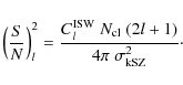
The total S/N is obtained after adding this contribution from l=2 up to l=lM given in Eq. (10):
In Fig. 6 we display the maximum l accessible by a cluster population driven from the Sheth-Tormen (Sheth & Tormen 1999) mass function in a WMAPV universe with
![\begin{figure}
\par\includegraphics[width=8cm,clip]{12525fg7.eps}
\vspace*{5mm}
\end{figure}](/articles/aa/full_html/2010/01/aa12525-09/img105.png)
|
Figure 7:
Top: angular number density of different cluster populations in different redshift shells of the width
|
| Open with DEXTER | |
In the top panel of Fig. 7 we display the actual angular density of those cluster populations at different redshifts, again for
![]() .
In the bottom panel, we display the required error in the peculiar velocity estimates (
.
In the bottom panel, we display the required error in the peculiar velocity estimates (
![]() )
in order to obtain a residual which is three times below the ISW level (i.e., S/N = 3). The symbol coding is the same as in the previous plot. For the cluster sample of
)
in order to obtain a residual which is three times below the ISW level (i.e., S/N = 3). The symbol coding is the same as in the previous plot. For the cluster sample of
![]() we require errors in the radial peculiar velocity of the order of 100-200 km s-1
in order to see the growth of the ISW at low redsfhits. These error
requirements become more stringent when more massive cluster
populations are used and when higher redshifts are to be probed. They
are at the level of the actual linear prediction for the kSZ in
clusters (
we require errors in the radial peculiar velocity of the order of 100-200 km s-1
in order to see the growth of the ISW at low redsfhits. These error
requirements become more stringent when more massive cluster
populations are used and when higher redshifts are to be probed. They
are at the level of the actual linear prediction for the kSZ in
clusters (![]() km s-1), so a priori are not too stringent. However, we must remark that these are the upper limits for the total
errors and should account for not only kSZ residuals, but also for
all other types of possible contaminants and systematics. Note as well
that the error on the kSZ recovery
km s-1), so a priori are not too stringent. However, we must remark that these are the upper limits for the total
errors and should account for not only kSZ residuals, but also for
all other types of possible contaminants and systematics. Note as well
that the error on the kSZ recovery ![]() is inversely proportional to the required S/N.
is inversely proportional to the required S/N.
5 Constraints on the cosmological dipole
Let us assume now that we include the dipole in the analyses to be
performed at the positions of the cluster distribution. The same
requirements which allow the tracing of the ISW growth should
permit us, a priori, to impose constraints on the intrinsic cosmological dipole of the same order, i.e., at the level of a few tens of ![]() K. Indeed, if we use Eq. (15) to impose
(S/N)l=1 = 1 with
K. Indeed, if we use Eq. (15) to impose
(S/N)l=1 = 1 with
![]() km s-1 and
km s-1 and
![]() K)2, we obtain
K)2, we obtain
![]()
![]() 103.
This is a relatively modest number of clusters: by including
all groups and clusters present in the different redshift shells,
the constraints on the cosmological dipole would improve even
further and could eventually yield a detection. With 4000 clusters
alone, the constraint of
103.
This is a relatively modest number of clusters: by including
all groups and clusters present in the different redshift shells,
the constraints on the cosmological dipole would improve even
further and could eventually yield a detection. With 4000 clusters
alone, the constraint of
![]() K
is between one and two orders of magnitude below the upper limit of the
cosmological dipole which can be inferred from our modelling of the
motion of the local group.
K
is between one and two orders of magnitude below the upper limit of the
cosmological dipole which can be inferred from our modelling of the
motion of the local group.
A natural question that arises in this context is how the subtraction
of the measured dipole (which includes both the intrinsic cosmological
dipole and the one induced by our peculiar motion) affects our
estimates of the intrinsic dipole in the positions of galaxy clusters.
Let us assume that the total dipole measured on the whole sphere is
built upon components of both the intrinsic cosmological and the observer's velocity dipoles. If, for the time being, we neglect all kSZ residuals in our subset of pixels containing clusters, ideally the total dipole measured at cluster positions would be
but in practice it will be
where the last component accounts for the errors introduced by our discrete cluster (pixel) distribution, and
That is, the rms error on the limits for the intrinsic cosmological dipole will be of the order
![\begin{displaymath}%
\left( \Delta [a^{\rm intr}_{1,m}] \right)^{1/2} \sim \frac...
...\epsilon_{l',m'} a_{l',m'}}{\langle \tau_{\rm T} \rangle}\cdot
\end{displaymath}](/articles/aa/full_html/2010/01/aa12525-09/img120.png)
According to this expression it becomes critical to choose a convenient cluster/pixel set that fulfills
6 Discussion and conclusions
Current CMB high angular resolution surveys like ACT or SPT are
scanning the sky at frequencies in which the identification of galaxy
clusters and groups should be possible via the tSZ and the
kSZ effects. Nominally, these experiments should be able to detect
via the tSZ all clusters more massive than 2 ![]()
![]() at large significance, but many smaller clusters and groups should
remain close to the detection threshold. Once clusters have been
identified by their tSZ distortion, attempts to detect the kSZ in
a subset of those systems can be conducted. The kSZ is our only probe
for peculiar velocities in the high redshift universe, and those can be
used themselves as probes for Dark Energy and missing baryons (Hernández-Monteagudo & Ho 2009; Hernández-Monteagudo et al. 2006).
In this context, a precise characterization and correction of all
possible contaminants is critical. The impact of the bSZ effect on
the kSZ amounts to
at large significance, but many smaller clusters and groups should
remain close to the detection threshold. Once clusters have been
identified by their tSZ distortion, attempts to detect the kSZ in
a subset of those systems can be conducted. The kSZ is our only probe
for peculiar velocities in the high redshift universe, and those can be
used themselves as probes for Dark Energy and missing baryons (Hernández-Monteagudo & Ho 2009; Hernández-Monteagudo et al. 2006).
In this context, a precise characterization and correction of all
possible contaminants is critical. The impact of the bSZ effect on
the kSZ amounts to ![]() %
for 10% of the clusters and groups, and becomes more important for
those objects with small radial projection in their peculiar motions.
Provided that the Thomson optical depth of the cluster is known,
this effect should be accurately predicted from background
CMB observations (as those available from e.g. WMAP or
Planck). The measurement of this effect is itself a measurement of the
gas content of the object under study.
%
for 10% of the clusters and groups, and becomes more important for
those objects with small radial projection in their peculiar motions.
Provided that the Thomson optical depth of the cluster is known,
this effect should be accurately predicted from background
CMB observations (as those available from e.g. WMAP or
Planck). The measurement of this effect is itself a measurement of the
gas content of the object under study.
This effect mirrors the CMB intensity at the epoch of
scattering, and this is relevant for secondary anisotropies which arise
at late times (like the ISW effect): a detection of the
bSZ effect in objects placed at different redshift shells would
provide the picture of the growth of the ISW at recent cosmological
times. The measurement we are proposing here is statistical,
and therefore it does not require a high S/N in each cluster (just in the same way as in Hernández-Monteagudo & Sunyaev 2008,
for the kSZ - E polarization mode cross correlation).
Our arguments here are therefore similar to those given in that work:
cluster and group positions can be inferred from observations in a wide
range of frequencies (optical, IR, X-ray, millimeter), many of which
are using those objects for studying the nature of Dark Energy. The
critical issue is the nature and the amplitude of residuals in the
kSZ/CMB estimation at the cluster positions. To what extent
do errors in the IR/radio point source
subtraction and/or in the characterization of the local peculiar
velocity field actually endanger the ISW measurements? This should
critically depend on whether those errors are systematic or not.
If those residuals can be regarded as independent
from cluster to cluster, the viability of this project should hinge
exclusively on the actual precision with which the point source and
kSZ residuals can be removed from the clusters' area. In this
regard, Diaferio et al. (2005) studied
the systematics that might arise when measuring kSZ fluctuations
at a cluster's position. Peculiar velocity reconstruction algorithms
based upon the local density field should be sensitive to the dark
matter peculiar velocity only. Diaferio et al. (2005) showed that, after averaging within the cluster's area, clusters/halos moving faster than 100 km s-1
show small differences in their dark matter - gas peculiar
velocities (around 10%). However, for those objects slower than
100 km s-1 this correction reached the level
of 90% and could pose a problem for the approach
suggested here. In that same work it is also shown that similar
uncertainties associated with peculiar motions of gas clumps and clouds
within the intra cluster medium may give rise to differences as large
as ![]() km s-1
between the halo's dark matter average peculiar velocity and the gas
peculiar velocity in different parts of the cluster. This aspect,
however, should be alleviated to great extent after integrating the
intensity over the cluster's area. Since the ISW contains most of
its power at low multipoles (lM <
10-20), targets may be chosen at a convenient distance in order to
minimize the required sky coverage. A possible strategy would then
consist of uniformly distributing
km s-1
between the halo's dark matter average peculiar velocity and the gas
peculiar velocity in different parts of the cluster. This aspect,
however, should be alleviated to great extent after integrating the
intensity over the cluster's area. Since the ISW contains most of
its power at low multipoles (lM <
10-20), targets may be chosen at a convenient distance in order to
minimize the required sky coverage. A possible strategy would then
consist of uniformly distributing
![]() patches in the sky (with
patches in the sky (with
![]() ), lying a distance
), lying a distance
![]() away and scanning deeply through each of those patches until finding a set of sources of high S/N
at different redshifts. This would improve the efficiency of the survey
(since a minimum amount of an area would be scanned) at the
expense however of improving the flux/mass thresholds shown in
Fig. 7. Hence one would
encounter here a trade-off between flux sensitivity and sky coverage.
Whatever approach is finally chosen, it should also provide strong
constraints on the cosmological dipole, which would be independent
from those imposed from the local dipole and the local velocity flows.
Let us also remark that this term has also been shown elsewhere (Khatri & Wandelt 2009) to be responsible for the generation of some level of non-Gaussianity due to the in-homogeneity of recombination.
away and scanning deeply through each of those patches until finding a set of sources of high S/N
at different redshifts. This would improve the efficiency of the survey
(since a minimum amount of an area would be scanned) at the
expense however of improving the flux/mass thresholds shown in
Fig. 7. Hence one would
encounter here a trade-off between flux sensitivity and sky coverage.
Whatever approach is finally chosen, it should also provide strong
constraints on the cosmological dipole, which would be independent
from those imposed from the local dipole and the local velocity flows.
Let us also remark that this term has also been shown elsewhere (Khatri & Wandelt 2009) to be responsible for the generation of some level of non-Gaussianity due to the in-homogeneity of recombination.
In this work we propose using for the first time the so-called blurring term in Thomson scattering for cosmological purposes. The small fraction of scattered off
CMB photons which are deviated when crossing a galaxy
cluster/group should provide information about what the
CMB anisotropy field was like at the time of the scattering.
If those objects are far away enough, the CMB at that epoch should
lack the ISW component that has arisen recently, and this
difference could a priori be picked up after removing all other
signals present in the cluster with enough accuracy. Assuming that
tSZ residuals are negligible, we find that a typical error of
100-200 km s-1 in the cluster peculiar velocity reconstruction is required for all clusters more massive than
![]() in order to trace the growth of the ISW at late times. These errors are
comparable with the linear expectations for the peculiar motions of
those objects, which involves that (i) the blurring correction to the kSZ is in general of relevance for the estimation of the latter and (ii) no very precise corrections for the kSZ are required. Those amplitudes roughly correspond to an error of 900-1800
in order to trace the growth of the ISW at late times. These errors are
comparable with the linear expectations for the peculiar motions of
those objects, which involves that (i) the blurring correction to the kSZ is in general of relevance for the estimation of the latter and (ii) no very precise corrections for the kSZ are required. Those amplitudes roughly correspond to an error of 900-1800
![]() K
per cluster. The same level of errors would provide stringent
constraints of the intrinsic cosmological dipole. Current and future
large scale structure surveys like eROSITA, Pan-STARRS, DES, PAU-BAO,
ACT or SPT should soon provide enough group and cluster candidates at
the relevant redshift ranges. Therefore, the critical point is the
feasibility of an accurate enough kSZ/tSZ/point source subtraction in
future high resolution CMB observations.
K
per cluster. The same level of errors would provide stringent
constraints of the intrinsic cosmological dipole. Current and future
large scale structure surveys like eROSITA, Pan-STARRS, DES, PAU-BAO,
ACT or SPT should soon provide enough group and cluster candidates at
the relevant redshift ranges. Therefore, the critical point is the
feasibility of an accurate enough kSZ/tSZ/point source subtraction in
future high resolution CMB observations.
References
- Abramo, L. R., & Xavier, H. S. 2007, Phys. Rev. D, 75, 101302 [NASA ADS] [CrossRef] [Google Scholar]
- Bardeen, J. M., Bond, J. R., Kaiser, N., & Szalay, A. S. 1986, ApJ, 304, 15 [NASA ADS] [CrossRef] [Google Scholar]
- Benitez, N., et al. 2008, ApJ, 691, 241 [Google Scholar]
- Challinor, A. D., Ford, M. T., & Lasenby, A. N. 2000, MNRAS, 312, 159 [NASA ADS] [CrossRef] [Google Scholar]
- Chluba, J., Hütsi, G., & Sunyaev, R. A. 2005, A&A, 434, 811 [Google Scholar]
- Cooray, A., & Baumann, D. 2003, Phys. Rev. D, 67, 063505 [NASA ADS] [CrossRef] [Google Scholar]
- Diaferio, A., Borgani, S., Moscardini, L., et al. 2005, MNRAS, 356, 1477 [NASA ADS] [CrossRef] [Google Scholar]
- Ettori, S., Morandi, A., Tozzi, P., et al. 2009, A&A, 501, 61 [Google Scholar]
- Giodini, S., Pierini, D., Finoguenov, A., et al. 2009, ApJ, 703, 982 [NASA ADS] [CrossRef] [Google Scholar]
- Hernández-Monteagudo, C., & Ho, S. 2009, MNRAS, 398, 790 [NASA ADS] [CrossRef] [Google Scholar]
- Hernández-Monteagudo, C., & Sunyaev, R. A. 2008, A&A, 490, 25 [Google Scholar]
- Hernández-Monteagudo, C., Verde, L., Jimenez, R., & Spergel, D. N. 2006, ApJ, 643, 598 [NASA ADS] [CrossRef] [Google Scholar]
- Inogamov, N. A., & Sunyaev, R. A. 2003, Astron. Lett., 29, 791 [NASA ADS] [CrossRef] [Google Scholar]
- Hincks, A. D., et al. 2009 [arXiv:0907.0461] [Google Scholar]
- Itoh, N., & Nozawa, S. 2004, A&A, 417, 827 [Google Scholar]
- Kamionkowski, M., & Loeb, A. 1997, Phys. Rev. D, 56, 4511 [NASA ADS] [CrossRef] [Google Scholar]
- Kashlinsky, A., Atrio-Barandela, F., Kocevski, D., & Ebeling, H. 2009, ApJ, 691, 1479 [NASA ADS] [CrossRef] [Google Scholar]
- Khatri, R., & Wandelt, B. D. 2009, Phys. Rev. D, 79, 023501 [NASA ADS] [CrossRef] [Google Scholar]
- Kitaura, F. S., & Enßlin, T. A. 2008, MNRAS, 389, 497 [NASA ADS] [CrossRef] [Google Scholar]
- Peel, A. C. 2006, MNRAS, 365, 1191 [NASA ADS] [CrossRef] [Google Scholar]
- Rephaeli, Y. 1995, ApJ, 445, 33 [NASA ADS] [CrossRef] [Google Scholar]
- Sachs, R. K., & Wolfe, A. M. 1967, ApJ, 147, 73 [NASA ADS] [CrossRef] [Google Scholar]
- Sazonov, S. Y., & Sunyaev, R. A. 1999, MNRAS, 310, 765 [NASA ADS] [CrossRef] [Google Scholar]
- Seljak, U., & Zaldarriaga, M. 1996, ApJ, 469, 437 [NASA ADS] [CrossRef] [Google Scholar]
- Seto, N., & Sasaki, M. 2000, Phys. Rev. D, 62, 123004 [NASA ADS] [CrossRef] [Google Scholar]
- Sheth, R. K., & Tormen, G. 1999, MNRAS, 308, 119 [NASA ADS] [CrossRef] [Google Scholar]
- Sheth, R. K., & Diaferio, A. 2001, MNRAS, 322, 901 [Google Scholar]
- Sunyaev, R. A., Norman, M. L., & Bryan, G. L. 2003, Astron. Lett., 29, 783 [NASA ADS] [CrossRef] [Google Scholar]
- Staniszewski, Z., Ade, P. A. R., Aird, K. A., et al. 2009, ApJ, 701, 32 [CrossRef] [Google Scholar]
- Sunyaev, R. A., & Zeldovich, Y. B. 1970, Ap&SS, 7, 3 [Google Scholar]
- Sunyaev, R. A., & Zeldovich, Y. B. 1972, Comments Astrophys. Space Phys., 4, 173 [NASA ADS] [EDP Sciences] [Google Scholar]
- Sunyaev, R. A., & Zeldovich, Y. B. 1980, MNRAS, 190, 413 [NASA ADS] [CrossRef] [Google Scholar]
- Sunyaev, R. A., & Zeldovich, Y. B. 1981, Astrophys. Space Phys. Rev., 1, 1 [NASA ADS] [Google Scholar]
- Vikhlinin, A., Kravtsov, A., Forman, W., et al. 2006, ApJ, 640, 691 [NASA ADS] [CrossRef] [Google Scholar]
- Yoshida, N., Sheth, R. K., & Diaferio, A. 2001, MNRAS, 328, 669 [NASA ADS] [CrossRef] [Google Scholar]
- Zeldovich, Y. B., & Sunyaev, R. A. 1969, Ap&SS, 4, 301 [Google Scholar]
- Zeldovich, Y. B., & Syunyaev, R. A. 1980, SvA Lett., 6, 285 [NASA ADS] [Google Scholar]
Footnotes
- ... WMAP
![[*]](/icons/foot_motif.png)
- WMAP's URL site: http:lambda.gsfs.nasa.gov/product/map/current/
- ... Planck
- Planck's URL site: http://www.esa.int/esaMI/Planck/index.html
- ... SPECTRUM-X/eROSITA
- Spectrum-X/eROSITA's URL site: http://www.mpe.mpg.de/projects.html#erosita
- ...=1,2,3
- This is not the case in Fourier space, where different spatial components of
 are correlated.
- ... (Pan-STARRS
- Pan-STARRS' URL site: http://pan-starrs.ifa.hawaii.edu/public/
- ... DES
- DES's URL site: http://www.darkenergysurvey.org/
- ... PAU-BAO
- PAU-BAO's URL site: http://www.ice.csic.es/research/PAU/
All Figures
|
|
Figure 1:
Fraction of the total CMB temperature rms that corresponds to scales
larger than the cluster size. The change of slope at
|
| Open with DEXTER | |
| In the text | |
|
|
Figure 2:
Top panel: total CMB map with two clusters for which the tSZ and the kSZ contributions have been removed. A high value of
|
| Open with DEXTER | |
| In the text | |
|
|
Figure 3:
a) Amplitude of the linear rms radial peculiar velocity in a WMAPV cosmology for a 2 |
| Open with DEXTER | |
| In the text | |
|
|
Figure 4: a) CMB TT angular power spectrum as seen by observers placed at redshifts z=0, 0.1, 1 and 2 (solid, dotted, dashed and dot-dashed lines, respectively). b) Same power spectra as in a) after being free streamed to the present moment. |
| Open with DEXTER | |
| In the text | |
|
|
Figure 5: Projection of the CMB quadrupole multipole a2,0 as seen by observers placed at different redshifts into different al,0 multipoles observed at present. Filled circles connected with a black solid line correspond to an observer placed at z=0.1, red triangles by a red dashed line to an observer at z=1 and green squares linked by a dot-dashed line to z=2. |
| Open with DEXTER | |
| In the text | |
|
|
Figure 6: Maximum multipole lM to which a discrete cluster sample in the full sky is sensitive (see Eq. (10)). The ISW is well contained within l< 30-40. |
| Open with DEXTER | |
| In the text | |
|
|
Figure 7:
Top: angular number density of different cluster populations in different redshift shells of the width
|
| Open with DEXTER | |
| In the text | |
Copyright ESO 2010
Current usage metrics show cumulative count of Article Views (full-text article views including HTML views, PDF and ePub downloads, according to the available data) and Abstracts Views on Vision4Press platform.
Data correspond to usage on the plateform after 2015. The current usage metrics is available 48-96 hours after online publication and is updated daily on week days.
Initial download of the metrics may take a while.