| Issue |
A&A
Volume 508, Number 2, December III 2009
|
|
|---|---|---|
| Page(s) | 565 - 574 | |
| Section | Cosmology (including clusters of galaxies) | |
| DOI | https://doi.org/10.1051/0004-6361/200912745 | |
| Published online | 01 October 2009 | |
A&A 508, 565-574 (2009)
Metal abundances in the cool cores of galaxy clusters![[*]](/icons/foot_motif.png)
S. De Grandi1 - S. Molendi2
1 - INAF - Osservatorio Astronomico di Brera,
via E. Bianchi 46, 23807 Merate (LC), Italy
2 -
INAF - IASF Milano,
via Bassini 15, 20133 Milano, Italy
Received 22 June 2009 / Accepted 27 August 2009
Abstract
We use XMM-Newton data to carry out a detailed
study of the Si, Fe and Ni abundances in the cool cores of a
representative sample of 26 local clusters. We performed a
careful evaluation of the systematic uncertainties related to the
instruments, the plasma codes and the spectral modeling, finding
that the major source of uncertainty is the plasma codes. Our
Si, Fe, Ni, Si/Fe and Ni/Fe distributions feature only moderate
spreads (from 20% to 30%) around their mean values strongly
suggesting similar enrichment processes at work in all our cluster
cores. Our sample-averaged Si/Fe ratio is comparable to those
measured in samples of groups and high luminosity ellipticals,
implying that the enrichment process in ellipticals, dominant
galaxies in groups and BCGs in clusters is quite similar. Although
our Si/Fe and Ni/Fe abundance ratios are fairly well constrained,
the large uncertainties in the supernova yields prevent us from
making a firm assessment of the relative contribution of type Ia
and core-collapsed supernovae to the enrichment process. All that
can be said with some certainty is that both contribute to
the enrichment of cluster cores.
Key words: X-rays: galaxies: clusters - galaxies: clusters: general - supernovae: general - galaxies: abundances - cooling flows - intergalactic medium
1 Introduction
The intra-cluster medium (ICM) that fills the deep potential well of
galaxy clusters is rich in metals. In the high mass regime of rich
clusters (
![]() ), where temperatures and
densities of the gas are of the order of 3-10 keV and 10-3 cm-3, respectively, the ICM is heavily ionized and the main
processes producing emission lines are collisions of ions with
electrons in a plasma in collisional ionization equilibrium. Since
the elements are well confined within the cluster potential well, they
accumulate over the whole cluster history and retain important
information on cluster formation and evolution. For gas temperatures
), where temperatures and
densities of the gas are of the order of 3-10 keV and 10-3 cm-3, respectively, the ICM is heavily ionized and the main
processes producing emission lines are collisions of ions with
electrons in a plasma in collisional ionization equilibrium. Since
the elements are well confined within the cluster potential well, they
accumulate over the whole cluster history and retain important
information on cluster formation and evolution. For gas temperatures
![]() 3 keV the most prominent emission lines are from He-like and
H-like K-shell transitions of Fe (at
3 keV the most prominent emission lines are from He-like and
H-like K-shell transitions of Fe (at ![]() 7 keV), along with less
pronounced K-shell lines of S, Si (at
7 keV), along with less
pronounced K-shell lines of S, Si (at ![]() 2 keV), Ar, Ca and Ni (at
2 keV), Ar, Ca and Ni (at ![]() 8 keV).
Temperature and abundances of the ICM are measured at the same time
from the X-ray spectrum: the temperature is measured from the
continuum emission that is almost entirely given by thermal
bremsstrahlung, whereas the abundance of an element is derived by
measuring the equivalent width of the line (once the continuum is
known), that is directly proportional to the ion-to-hydrogen
concentration ratio (see Kaastra et al. 2008, for a review of the thermal radiation
processes in clusters).
While in principle the abundance measurement is straightforward, in
practice various sources of uncertainties are present, amongst which
(1) the accuracy of the atomic physics; (2) the moderate spectral
resolution of the current imaging instruments which often results in
line blending; this is particularly severe for L-shell blends where
the transitions are not entirely understood; (3) the presence of
temperature gradients in the ICM, especially in the cluster cores,
that need specific spectral modeling.
With the advent of the Chandra and XMM-Newton satellite,
carrying detectors with both high spatial and spectral capabilities,
the statistical quality of cluster spectra (in particular for
cool core regions) improved dramatically. While on the one hand the
statistical errors associated with the abundance measurements have
greatly decreased, on the other hand surprisingly little attention has been
devoted to systematic sources of uncertainties which, under these
circumstances, are likely to play an important role.
8 keV).
Temperature and abundances of the ICM are measured at the same time
from the X-ray spectrum: the temperature is measured from the
continuum emission that is almost entirely given by thermal
bremsstrahlung, whereas the abundance of an element is derived by
measuring the equivalent width of the line (once the continuum is
known), that is directly proportional to the ion-to-hydrogen
concentration ratio (see Kaastra et al. 2008, for a review of the thermal radiation
processes in clusters).
While in principle the abundance measurement is straightforward, in
practice various sources of uncertainties are present, amongst which
(1) the accuracy of the atomic physics; (2) the moderate spectral
resolution of the current imaging instruments which often results in
line blending; this is particularly severe for L-shell blends where
the transitions are not entirely understood; (3) the presence of
temperature gradients in the ICM, especially in the cluster cores,
that need specific spectral modeling.
With the advent of the Chandra and XMM-Newton satellite,
carrying detectors with both high spatial and spectral capabilities,
the statistical quality of cluster spectra (in particular for
cool core regions) improved dramatically. While on the one hand the
statistical errors associated with the abundance measurements have
greatly decreased, on the other hand surprisingly little attention has been
devoted to systematic sources of uncertainties which, under these
circumstances, are likely to play an important role.
In this paper, our first goal is to provide a robust measurement of the distribution of abundances and abundance ratios of the chemical elements in the cores of a representative sample of nearby and bright cool core clusters. In this context, ``robust estimate'' essentially means that we will include in the error budget a careful evaluation of the systematic uncertainties potentially affecting our data. We will consider both instrument related systematics and plasma code systematics. We stress that in this paper we are interested in the measure of the global abundances in the central region of each cluster, not in the analysis of radial profiles. Moreover, these central regions will provide us with the maximum photon statistics because of their very intense central surface brightness peaks, thereby allowing us to explore the most subtle sources of systematic errors and reliably measure the most abundant elements observable in the ICM (e.g. Si, Fe and Ni).
The elements observed in the ICM are produced through thermo-nuclear
nucleo-synthesis in supernova (SN) explosions occurring in the member
early-type galaxies (Renzini et al. 1993; Arnaud et al. 1992), and they are
eventually ejected/diffused into the ICM through galactic winds
(for a review see Bland-Hawthorn et al. 2007) and ram pressure
stripping (e.g. Schindler & Diaferio 2008, and references therein).
Supernovae are classified on the basis of their progenitor
models. Two main groups of SNe are known: type Ia supernovae
(SNIa) that are derived from an accreting white dwarf in a binary system,
and core-collapsed supernovae (SNcc) whose progenitors are single
massive stars (![]()
![]() ). One of the most important
quantities that theoretical models of SNe provide are the yields of the
various chemical elements, namely the mass per element and per SN
event. While SNIa produce mostly Fe, Ni and Si-group metals (i.e.
Si, S, Ar, Ca), the SNcc ejecta are rich in
). One of the most important
quantities that theoretical models of SNe provide are the yields of the
various chemical elements, namely the mass per element and per SN
event. While SNIa produce mostly Fe, Ni and Si-group metals (i.e.
Si, S, Ar, Ca), the SNcc ejecta are rich in ![]() -elements (i.e. O,
Ne, Mg, as well as few Si-group elements).
In the 90 s BeppoSAX and ASCA observations revealed that
the centers of cool core clusters always display an excess (with
respect to the external cluster regions) of Fe around the central
cluster galaxy
(e.g. Leccardi & Molendi 2008a; De Grandi & Molendi 2001; Fukazawa et al. 2000). The iron mass
inferred from this excess is consistent with it being entirely produced
by the giant galaxy itself (e.g. Böhringer et al. 2004; De Grandi et al. 2004),
which is always found in these systems. Other elements such as Mg, Si
and S show abundance peaks in cluster cores
(e.g. Finoguenov et al. 2000; Tamura et al. 2004; Fukazawa et al. 1998; Sato et al. 2009a; Finoguenov et al. 2001).
Under the assumption that the sole sources of metals are the two types
of SNe, observations of the
-elements (i.e. O,
Ne, Mg, as well as few Si-group elements).
In the 90 s BeppoSAX and ASCA observations revealed that
the centers of cool core clusters always display an excess (with
respect to the external cluster regions) of Fe around the central
cluster galaxy
(e.g. Leccardi & Molendi 2008a; De Grandi & Molendi 2001; Fukazawa et al. 2000). The iron mass
inferred from this excess is consistent with it being entirely produced
by the giant galaxy itself (e.g. Böhringer et al. 2004; De Grandi et al. 2004),
which is always found in these systems. Other elements such as Mg, Si
and S show abundance peaks in cluster cores
(e.g. Finoguenov et al. 2000; Tamura et al. 2004; Fukazawa et al. 1998; Sato et al. 2009a; Finoguenov et al. 2001).
Under the assumption that the sole sources of metals are the two types
of SNe, observations of the ![]() -elements/Fe abundance ratios
coupled with the knowledge of the SNe chemical yields allow the
determination of the SNIa and SNcc proportion within each cluster.
Finoguenov et al. (2000) found an increasing Si/Fe ratio with radius
in clusters, indicating a greater predominance of SNcc enrichment at
large radii, while the innermost parts appeared dominated by SNIa
products. However, work based on data taken with the more recent XMM-Newton and SUZAKU observatories have not fully confirmed
this overall picture for rich clusters. Tamura et al. (2004), studying the
spatial distributions of metals in a sample of cool core clusters
observed with XMM-Newton, found uniform Si/Fe and S/Fe ratios
within the ICM, but increasing O/Fe (although this ratio was prone to
large uncertainties). SUZAKU observations confirm these findings
(e.g. Sato et al. 2007a; Matsushita & Suzaku SWG team 2008).
The relative proportion of SNIa and SNcc found by XMM-Newton and
SUZAKU observations are in rough agreement (Sato et al. 2007a),
although these results were achieved using of specific collections of
SNe yields (e.g. Nomoto et al. 2006; Iwamoto et al. 1999). None of the
combinations of the theoretical SNIa and SNcc yields available in the
literature have reproduced the overall elemental pattern in cluster
cores (fits were not formally acceptable based on the
-elements/Fe abundance ratios
coupled with the knowledge of the SNe chemical yields allow the
determination of the SNIa and SNcc proportion within each cluster.
Finoguenov et al. (2000) found an increasing Si/Fe ratio with radius
in clusters, indicating a greater predominance of SNcc enrichment at
large radii, while the innermost parts appeared dominated by SNIa
products. However, work based on data taken with the more recent XMM-Newton and SUZAKU observatories have not fully confirmed
this overall picture for rich clusters. Tamura et al. (2004), studying the
spatial distributions of metals in a sample of cool core clusters
observed with XMM-Newton, found uniform Si/Fe and S/Fe ratios
within the ICM, but increasing O/Fe (although this ratio was prone to
large uncertainties). SUZAKU observations confirm these findings
(e.g. Sato et al. 2007a; Matsushita & Suzaku SWG team 2008).
The relative proportion of SNIa and SNcc found by XMM-Newton and
SUZAKU observations are in rough agreement (Sato et al. 2007a),
although these results were achieved using of specific collections of
SNe yields (e.g. Nomoto et al. 2006; Iwamoto et al. 1999). None of the
combinations of the theoretical SNIa and SNcc yields available in the
literature have reproduced the overall elemental pattern in cluster
cores (fits were not formally acceptable based on the ![]() values; e.g. Sato et al. 2007a; Baumgartner et al. 2005; de Plaa et al. 2007). There are at
least two possible solutions to this problem: the existence of an
additional source of elements other than SNIa and SNcc
(see Finoguenov et al. 2002; Baumgartner et al. 2005; Mannucci et al. 2006), or, the need for
a revision of the theoretical SNe models (e.g. Young & Fryer 2007).
Interestingly, a systematic exploration of the full range of
uncertainties of theoretical yields was last provided by
Gibson et al. (1997), although since then, several new compilations of
SNcc yields have become available (e.g. Chieffi & Limongi 2004; Nomoto et al. 2006)
along with new yields for SNIa (Iwamoto et al. 1999). As pointed out by
Gibson et al. (1997), the relative contribution of SNIa and SNcc to the Fe
abundance in the ICM depends crucially upon the adopted theoretical
SNe models.
values; e.g. Sato et al. 2007a; Baumgartner et al. 2005; de Plaa et al. 2007). There are at
least two possible solutions to this problem: the existence of an
additional source of elements other than SNIa and SNcc
(see Finoguenov et al. 2002; Baumgartner et al. 2005; Mannucci et al. 2006), or, the need for
a revision of the theoretical SNe models (e.g. Young & Fryer 2007).
Interestingly, a systematic exploration of the full range of
uncertainties of theoretical yields was last provided by
Gibson et al. (1997), although since then, several new compilations of
SNcc yields have become available (e.g. Chieffi & Limongi 2004; Nomoto et al. 2006)
along with new yields for SNIa (Iwamoto et al. 1999). As pointed out by
Gibson et al. (1997), the relative contribution of SNIa and SNcc to the Fe
abundance in the ICM depends crucially upon the adopted theoretical
SNe models.
The second main goal of this paper is to provide a critical assessment of the relative contributions of the SNIa versus SNcc to the enrichment process. Contrary to other similar works present in the recent literature (e.g. de Plaa et al. 2007), we do not neglect the uncertainties associated with the current theoretical yields and explore how they affect the derived SNIa fraction.
This paper is organized as follows. In Sect. 2 we present the sample, in Sect. 3 we describe the cleaning process of the raw XMM-Newton archival data, and, in Sect. 4, we concentrate on the spectral analysis and on the choice of the best fitting model. In Sect. 4 we also discuss the systematic uncertainties related to imperfections in the cross-calibration between the three EPIC instruments. In Sect. 5 we present results on the derived distributions of metal abundances and abundance ratios. In this same section we compare results from two different choices for the spectral codes. In Sect. 6 we discuss the relative contribution to the overall enrichment process of different SNe types. In Sect. 7 we discuss our findings and in Sect. 8 we summarize our main results.
We assume H0 = 70 km s-1 Mpc-1 and
![]() ;
the source redshifts are all extracted from
the NASA/IPAC Extragalactic Database (NED). All metallicity
measurements we show in this paper are relative to the photospheric
solar abundances of Anders & Grevesse (1989). In this set of abundances, Fe
has a number density of
;
the source redshifts are all extracted from
the NASA/IPAC Extragalactic Database (NED). All metallicity
measurements we show in this paper are relative to the photospheric
solar abundances of Anders & Grevesse (1989). In this set of abundances, Fe
has a number density of
![]() ,
Si
,
Si
![]() and Ni
and Ni
![]() ,
all number densities are relative to
H. All uncertainties shown are
,
all number densities are relative to
H. All uncertainties shown are ![]() confidence level (i.e.
confidence level (i.e.
![]() ).
).
2 The sample
Starting from the flux-limited sample of 55 galaxy clusters listed by Edge et al. (1990) and the ROSAT PSPC analysis of this sample performed by Peres et al. (1998), we have selected all the objects with a mass deposition rate different from zero (see Table 5 in Peres et al. 1998). Among these clusters we have chosen all those that were observed with XMM-Newton EPIC within April 2008, with the exclusion of clusters whose observations are strongly affected by soft protons (e.g. Abell 644 and Abell 2142). The 32 clusters that meet these requirements are listed in Table 1 (available online only).
3 Data preparation
We reprocessed the Observation Data Files (ODF) using the Science Analysis System (SAS) version 7.0.0. After the production of the calibrated event lists for the EPIC MOS1, MOS2 and pn observations with emchain and epchain tasks, we performed a soft proton cleaning using a double filtering process.
We first removed soft protons spikes by screening the light curves
produced in 100 bins in the 10-12 keV band and applying an appropriate
threshold for each instrument, generally a threshold of 0.20 cts s-1 for MOS1 and MOS2, and of 0.60 cts s-1 for pn.
Then to eliminate possible residual flares contributing below
10 keV, we extracted a light curve in the 2-5 keV band and
fitted the
histogram produced from this curve with a Gaussian distribution. To
generate the final filtered event file we rejected all events
registered at times when the count rate was more than ![]() from
the mean of this distribution. Finally, we filtered event files
according to FLAG (FLAG==0) and PATTERN (PATTERN
from
the mean of this distribution. Finally, we filtered event files
according to FLAG (FLAG==0) and PATTERN (PATTERN ![]() 12 for MOS and
PATTERS==0 for pn) criteria. The resulting effective exposure
times of the observations are reported in Table 1
(available online only).
12 for MOS and
PATTERS==0 for pn) criteria. The resulting effective exposure
times of the observations are reported in Table 1
(available online only).
Using the cleaned event files we extracted spectra from a
circular region centered on the cluster emission peaks. The physical
radius of this region is 0.5
![]() ,
where
,
where
![]() is
the cooling radius computed by Peres et al. (1998). With this choice of
the extraction radius, we sample a significative portion of the cool
core and we assure that the extracted region is contained within the
EPIC field of view for all our clusters. Prominent point-like sources
have been removed from the extraction region. Other authors
(e.g. Rasmussen & Ponman 2007; de Plaa et al. 2007) select their extraction regions
as fixed fractions of the cluster scaling radius,
e.g. de Plaa et al. (2007) used 0.2 of r500, where r500 is the radius
encompassing a spherical density contrast of 500 with respect to the
critical density. By converting our extraction radii in r500units we find a rather peaked distribution centered around 0.08 r500.
is
the cooling radius computed by Peres et al. (1998). With this choice of
the extraction radius, we sample a significative portion of the cool
core and we assure that the extracted region is contained within the
EPIC field of view for all our clusters. Prominent point-like sources
have been removed from the extraction region. Other authors
(e.g. Rasmussen & Ponman 2007; de Plaa et al. 2007) select their extraction regions
as fixed fractions of the cluster scaling radius,
e.g. de Plaa et al. (2007) used 0.2 of r500, where r500 is the radius
encompassing a spherical density contrast of 500 with respect to the
critical density. By converting our extraction radii in r500units we find a rather peaked distribution centered around 0.08 r500.
![\begin{figure}
\par\mbox{\includegraphics[width=4.5cm,angle=-90]{12745f1a.ps} \i...
...f1e.ps} \includegraphics[width=4.8cm,angle=-90]{12745f1f.ps} }
\end{figure}](/articles/aa/full_html/2009/47/aa12745-09/img18.png)
|
Figure 1: EPIC- pn spectral data (crosses) and best-fit models (continuum lines) for 3 high counting statistics clusters: Perseus (on the top), 2A 0335+096 (in the middle) and Centaurus (at the bottom). Panels on the left show results from a 4T model fit without Gaussian smoothing whereas plots on the right are smoothed. In all cases we also plot the data divided by the folded model. The spectra are rebinned for clarity. The energy range of each plot is 600 eV centered on the 6.7 keV line (redshifted at the cluster distance). In the panels on the left the ``wings'' around the Fe line are clearly visible in the residuals, an indication of the resolution mis-calibration of the redistribution matrix of the pn (see discussion in Sect. 4.1). |
| Open with DEXTER | |
4 Spectral analysis
In this paper we wish to measure abundances for Si, Fe and Ni. To
achieve robust estimates, we choose to make our measures from the
K-shell lines only, avoiding L-shell blends where uncertainties
associated with the atomic physics are larger. We achieve this by
setting a lower energy threshold of 1.8 keV which includes Si K-shell
emission (2 keV) and excludes the Fe and Ni L-shell blends (![]() 1.-1.5 keV).
1.-1.5 keV).
The background subtraction for the high surface brightness core
regions of cool core clusters is less critical than in the case of
more external low surface brightness regions. We therefore
decided to subtract the background using blank-sky fields instead of
proceeding with a more detailed modeling of the different background
components. The blank-sky fields for EPIC MOS and pn were
produced by Leccardi & Molendi (2008a) (see Appendix B ``The analysis
of blank field observations'' in their paper) by analysing a large
number of observations for a total exposure time of ![]() 700 ks for
MOS and
700 ks for
MOS and ![]() 500 ks for pn.
500 ks for pn.
We refined our background analysis by also performing a background
rescaling for each observation separately to account for temporal
variations of the background. We estimated the background intensity
from spectra extracted from an external ring between ![]() and
and
![]() centered on the emission peak, taking into account only
the 10-12 keV band (to avoid possible extended cluster emission
residuals in this region). We then rescaled the blank-sky fields
background to the local value. This procedure is especially important
when deriving the nickel abundance from its emission lines at
centered on the emission peak, taking into account only
the 10-12 keV band (to avoid possible extended cluster emission
residuals in this region). We then rescaled the blank-sky fields
background to the local value. This procedure is especially important
when deriving the nickel abundance from its emission lines at ![]() 8 keV. Indeed, in this hard spectral region, both the EPIC effective area
and the surface brightness of the relatively low temperature cluster
cores decrease rapidly, and the background becomes progressively more
important.
8 keV. Indeed, in this hard spectral region, both the EPIC effective area
and the surface brightness of the relatively low temperature cluster
cores decrease rapidly, and the background becomes progressively more
important.
All the spectral fits were performed with the XSPEC package (version 11.3.2, Arnaud 1996).
We analyzed each cluster spectrum with three different models: (1) a one temperature thermal model with the plasma in collisional ionization equilibrium (vmekal model in the XSPEC nomenclature), referred to as the 1T model hereafter; (2) a two temperature thermal model (vmekal+vmekal), 2T model hereafter, and; (3) a multi-temperature model (vmekal+vmekal+vmekal+vmekal), 4T model hereafter.
All models were multiplied by the Galactic hydrogen column
density, ![]() ,
determined by HI surveys (Kalberla et al. 2005) through the
wabs absorption model in XSPEC. In the following sections we
report results from spectral fits with
,
determined by HI surveys (Kalberla et al. 2005) through the
wabs absorption model in XSPEC. In the following sections we
report results from spectral fits with ![]() fixed at the weighted
Galactic value only. We have also allowed
fixed at the weighted
Galactic value only. We have also allowed ![]() to vary in all three
models finding no significant differences in the derived silicon, iron
and nickel abundance values.
to vary in all three
models finding no significant differences in the derived silicon, iron
and nickel abundance values.
The redshifts are taken from the NASA/IPAC Extragalactic Database and were always left as free parameters to account for small calibration differences between the two MOS and the pn cameras. We have allowed the temperatures of 1T and 2T models to vary freely, whereas in the 4T model temperatures of the four components were fixed at 1, 2, 4 and 8 keV, respectively. The normalizations of the models and the elements Si, S, Fe and Ni were left free to vary. Ar and C were joined to S as these elements are less abundant and we do not plan to study them in the course of this work.
As pointed out by Leccardi & Molendi (2008a), when fitting spectra with XSPEC it is appropriate to allow the metallicities to assume negative values. This procedure is necessary to avoid underestimates on the derived metal abundances which could affect the measurements, especially for the case of low metallicity, statistically poor spectra (for a more detailed discussion of this point see Appendix A in Leccardi & Molendi 2008a).
Abundances are measured relative to the solar photospheric values of
Anders & Grevesse (1989), where Fe
![]() ,
Si
,
Si
![]() and Ni
and Ni
![]() (by number relative
to H). We have chosen these values to allow direct comparison with
other works present in the literature. Spectra from all three EPIC
instruments (MOS1, MOS2 and pn) were fitted individually.
(by number relative
to H). We have chosen these values to allow direct comparison with
other works present in the literature. Spectra from all three EPIC
instruments (MOS1, MOS2 and pn) were fitted individually.
In the course of our analysis, we found that spectra with less than about 3500 source counts could not be used to constrain the abundances of nickel and silicon, therefore we decided to eliminate from the sample all clusters having less than 3500 source counts in the adopted energy band (i.e. 1.8-10 keV) in at least one of the three EPIC instruments. The five clusters removed from the sample by adopting this criterion are: Abell 1644, Abell 1651, Abell 2065, Abell 2063 and Abell 3562.
We have also excluded Cygnus A because of its peculiar core emission. A powerful double-lobed radio galaxy, QSO B1957+405, featuring huge jets feeding very large hotspot regions which are well detected in X-rays resides in the core of this cluster. In the light of the difficulty of removing efficiently the emission associated with the radio galaxy from the spectra of the core region we preferred to exclude this cluster from the sample.
In the case of the nickel abundance measurement, we introduced a
further selection criterion to exclude clusters that are background
dominated in the hard part of the spectrum. We selected the 7-9 keV
energy band redshifted at the cluster distance around the nickel line
at ![]() 8 keV, and we have measured the relative difference between
the source and background count rates,
8 keV, and we have measured the relative difference between
the source and background count rates,
![]() ,
in that band. We then considered only nickel measurements from
clusters with relative difference larger than 1, namely clusters with
source count rates which were at least twice the background count
rate in the hard band. Applying this selection Virgo, Abell 262
and Abell 1060 are also excluded from the sample.
Our pn spectra are only mildly contaminated by the fluorescence
line complex located around 8 keV (e.g. Ness et al. 2009), the
reason being that our spectra are extracted from the central regions
of the pn detector where, due to a hole in the pn
electronics box, the fluorescence lines are weak.
,
in that band. We then considered only nickel measurements from
clusters with relative difference larger than 1, namely clusters with
source count rates which were at least twice the background count
rate in the hard band. Applying this selection Virgo, Abell 262
and Abell 1060 are also excluded from the sample.
Our pn spectra are only mildly contaminated by the fluorescence
line complex located around 8 keV (e.g. Ness et al. 2009), the
reason being that our spectra are extracted from the central regions
of the pn detector where, due to a hole in the pn
electronics box, the fluorescence lines are weak.
In summary we have measured Si and Fe abundances from a sample of 26 clusters and Ni from a subsample of 23 systems.
4.1 Addendum to the spectral analysis of the pn
Molendi & Gastaldello (2009), analyzing the pn spectra of
a long XMM-Newton observation of the Perseus cluster, first
noted in the best-fit residuals the presence of a substantial
structure around the Fe K![]() line (see Sect. 3.1.1 and Fig. 2 in
their paper). This structure is attributed to an incorrect modeling of
the pn spectral resolution within the redistribution matrix.
line (see Sect. 3.1.1 and Fig. 2 in
their paper). This structure is attributed to an incorrect modeling of
the pn spectral resolution within the redistribution matrix.
Investigating this features extensively in the pn spectra of our
cluster sample, we found that the resolution mis-calibration can be
compensated for by including a multiplicative component that performs
a Gaussian smoothing of the spectral model (gsmooth in
XSPEC). We set the width of the Gaussian kernel to be 4 eV (FWHM) at 6 keV and assume a power-law dependency of the width on the energy with
an index of ![]() 1.
1.
Figure 1 shows the pn spectra and best-fit
residuals for three bright clusters: Perseus, 2A 0335+096 and
Centaurus clusters. We have fitted the spectra with the 4T model
without and with the Gaussian smoothing. In the former cases (left
panels in the figure), prominent residuals are present in the
``wings'' of the Fe line, while in the latter (right panels) the
residuals are significantly reduced.
In 13 (11) out of 26 cases the modified models
applied to pn spectra provide a substantially better fit (i.e.
![]() )
than the unmodified models. We note that
Si and Ni lines do not show similar residuals with respect to the best
fit model, most likely because the statistical quality of the data is
not as high (Si and Ni) and because the spectral resolution is
significantly poorer (Si).
)
than the unmodified models. We note that
Si and Ni lines do not show similar residuals with respect to the best
fit model, most likely because the statistical quality of the data is
not as high (Si and Ni) and because the spectral resolution is
significantly poorer (Si).
After the application of the Gaussian smoothing, the
cross-calibrations between the pn and MOS improve. For
instance, the relative differences, computed over the whole sample,
between iron abundances estimated from pn and MOS1 spectra, i.e.
![]() ,
with the un-smoothed and
smoothed 4T model decrease from
,
with the un-smoothed and
smoothed 4T model decrease from ![]() to
to ![]() ,
whereas the ones
between pn and MOS2 decrease from
,
whereas the ones
between pn and MOS2 decrease from ![]() to
to ![]() (errors on the
given percentages are always
(errors on the
given percentages are always ![]() ).
).
4.2 Choice of the best spectral model for each cluster
In this section we discuss how we selected the model that best fits the spectral data among the 1T, 2T and 4T models described above.
Applying the statistical F-test between 1T and 2T (or 1T and 4T)
models, we find that only the first 6 out of 26 clusters with larger
statistics (i.e. Perseus, Virgo, 2A 0335+96, Centaurus, Abell 478
and Abell 4038) show overwhelming evidence of multi-temperature
structure, namely an F-test probability, PF, smaller than ![]() for
all EPIC instruments.
for
all EPIC instruments.
The majority of the other clusters (17/26 for 2T model and 22/26 for
4T model), however, show a significant improvement (![]() )
in at
least one of the EPIC instruments. For these clusters, the relative
differences between the metal abundances measured in each instrument
with the 1T and 2T (or 1T and 4T) models are always smaller than
2-3
)
in at
least one of the EPIC instruments. For these clusters, the relative
differences between the metal abundances measured in each instrument
with the 1T and 2T (or 1T and 4T) models are always smaller than
2-3![]() for Fe and Si, and consistent with zero for Ni.
Therefore, from a purely statistical point of view, the choice of 1T
or multi-temperature (2T or 4T) models results in modest differences.
Nevertheless, we point out that our spectra are extracted from the
very central regions of cool core clusters and that these regions
always display temperature gradients (e.g. Leccardi & Molendi 2008b, and
references therein). It follows that the best description of the
spectrum of this plasma is through a multi-temperature model. For
this reason and from the F-test results above, we decide to use a
multi-temperature modeling for all the clusters in the sample.
for Fe and Si, and consistent with zero for Ni.
Therefore, from a purely statistical point of view, the choice of 1T
or multi-temperature (2T or 4T) models results in modest differences.
Nevertheless, we point out that our spectra are extracted from the
very central regions of cool core clusters and that these regions
always display temperature gradients (e.g. Leccardi & Molendi 2008b, and
references therein). It follows that the best description of the
spectrum of this plasma is through a multi-temperature model. For
this reason and from the F-test results above, we decide to use a
multi-temperature modeling for all the clusters in the sample.
An F-test between 2T and 4T models is not possible as the two models
have the same numbers of degrees of freedom. However, relative
differences between the metal abundances measured with the two models
show that the systematic uncertainties associated with the different
modeling of the data are below ![]() for Fe and Si and consistent
with zero for Ni. These systematic errors are of the same order as or
smaller than the systematic errors on the abundances due to
calibration differences between the three EPIC detectors (systematic
errors given by the cross correlation between EPIC instruments will be
discussed in Sect. 4.3). Therefore the two models are equivalent to
describe our data. We choose to use the 4T model for all the clusters.
for Fe and Si and consistent
with zero for Ni. These systematic errors are of the same order as or
smaller than the systematic errors on the abundances due to
calibration differences between the three EPIC detectors (systematic
errors given by the cross correlation between EPIC instruments will be
discussed in Sect. 4.3). Therefore the two models are equivalent to
describe our data. We choose to use the 4T model for all the clusters.
4.3 EPIC cross-calibration issues
For each cluster we compute the relative differences between iron, silicon, and nickel measured with MOS1, MOS2 and pn, and subsequently compute the weighted averages of these differences for the whole sample (i.e. 26 clusters for Fe and Si, and 23 clusters for Ni, results are from 4T model). The resulting mean values for Si, Fe and Ni are shown in Table 2 (available online only). From the results shown in this table it is clear that systematic errors are often dominant with respect to statistical ones for Fe and Si, whereas Ni appears to be fully dominated by statistical uncertainties. Another important point is that the relative differences between MOS1 and MOS2 are smaller than the differences between MOS1 or MOS2 and pn.
To account for systematic differences between measures obtained from
different detectors and spectral models we add in quadrature a 3%
systematic error to each Fe and Si abundance measurement. The
relative differences between iron, silicon, and nickel measured with
MOS1, MOS2 and pn computed over the whole sample, including the
3% systematic errors, are smaller than those computed without them
and are always significant at less than 3![]() (these values are
given in the second line relative to each element in Table 2).
(these values are
given in the second line relative to each element in Table 2).
For each cluster we compute an EPIC Fe and Si abundance by performing
error weighted averages over the three detectors, with errors
including the 3% systematic error described above. Errors on the EPIC Fe
and Si abundances are computed by dividing the error weighted standard
deviation of the EPIC abundance by the square root of 3. To avoid
errors on the EPIC abundances from falling below the systematic level,
a ![]() systematic error is summed in quadrature.
systematic error is summed in quadrature.
As shown in Table 2, nickel measurements are clearly dominated by statistical errors, nevertheless we decided for internal consistency to compute the nickel value for each cluster as described above for Si and Fe. Indeed we expect Ni to be prone to the same systematics affecting Si and Fe.
The distribution of Fe and Si abundances is not very symmetric, which means that it is not particularly well represented by a Gaussian. We determined that the major cause is the presence of a few measurements with extremely small errors. Introducing a systematic error of 3% (see above) alleviates the problem considerably. The fact that the data is not normally distributed can be observed in Table 2: the Fe abundance measured with mekal, although the mean relative difference for MOS1 and MOS2 measures is small (2%), and the mean relative difference for MOS1 and pn is large, (7%), the mean relative difference for MOS2 and pn is modest, i.e. 2%. Similar results are observed for Si measured with mekal and with Fe and Si measured with apec.
The final abundances are reported in Table 3
(available online only): Col. (1) is the cluster name,
Cols. (2)-(4) are the EPIC error weighted averages of Si, Fe and
Ni,
respectively, with their ![]() errors.
errors.
For completeness we have also computed all the abundances presented in
Table 3 using the 2T model; as expected, we found only
modest differences with respect to those estimated with the 4T
model. The relative differences between the mean Fe, Si and Ni values
computed for the whole sample with the 2T and 4T models are
![]() ,
,
![]() and
and
![]() ,
respectively. In the case of Fe
we detect a systematic error that is of the same order as the one
associated with the choice of detector, while in the case of Si and Ni
the indeterminations are sufficiently large to hide systematic errors
of the same order.
,
respectively. In the case of Fe
we detect a systematic error that is of the same order as the one
associated with the choice of detector, while in the case of Si and Ni
the indeterminations are sufficiently large to hide systematic errors
of the same order.
4.4 apec vs. mekal
Mekal is not the only collisional ionization equilibrium (CIE)
emission model in XSPEC. An alternative plasma code known as apec (Smith et al. 2001) is available. Some authors have
performed comparisons between spectral fits performed with the two
codes (e.g. Sanders & Fabian 2006; de Plaa et al. 2007).
Sanders & Fabian (2006), analyzing a long Chandra observation
of the core of Centaurus, found that while there are few differences
between Si and Fe abundances estimated with the two codes, the Ni
abundance found with apec is somewhat smaller than that found
with mekal, a similar result, albeit with less statistical
strength, was found by de Plaa and collaborators. Here we wish to
investigate how the differences between the plasma codes impact on our
abundance and abundance ratio measurements. To this end, we reanalyzed
all our objects with a multi-temperature model (vapec+vapec+vapec+vapec) analogous to the 4T mekal model which
we call 4T apec. A comparison amongst apec metal
abundances measured with the three EPIC instruments (see Table
2, available online only) provides results that
are very similar to those found for mekal; including a
systematic error of 3% on the measures alleviates the difference
between the three instruments in much the same way (see Table
2) as it does for the 4T mekal fits. Mean metal
abundances for Si, Fe and Ni and abundance ratios, Si/Fe and Ni/Fe
obtained with apec and associated intrinsic scatters are
reported in Table 4 (available online only). Comparing
the sample average metal abundances measured with mekal with
those obtained with apec we find that: Fe is almost unchanged,
Feapec/Fe
![]() ;
Si is somewhat higher,
Siapec/Si
;
Si is somewhat higher,
Siapec/Si
![]() and Ni is lower,
Niapec/Ni
and Ni is lower,
Niapec/Ni
![]() .
The Si/Fe ratio, as measured
with apec, is slightly higher than that estimated with mekal, (Si/Fe)apec/(Si/Fe)
.
The Si/Fe ratio, as measured
with apec, is slightly higher than that estimated with mekal, (Si/Fe)apec/(Si/Fe)
![]() ,
while Ni/Fe
is substantially lower, (Ni/Fe)apec/(Ni/Fe)
,
while Ni/Fe
is substantially lower, (Ni/Fe)apec/(Ni/Fe)
![]() .
.
In summary, while for Fe and Si/Fe the systematic error associated with the cross-calibration between EPIC experiments, 3%, are comparable to those related to the emission model, 5% and 6% respectively, for Si, Ni, and for Ni/Fe the dominant source of error is the systematics related to the emission model, 11%, 18% and 23% respectively. The statistical errors on the mean Si, Fe, Ni, Si/Fe and Ni/Fe are always dominated by systematic errors.
5 Abundance results in cool cores
5.1 Mean iron, silicon and nickel abundances
In Fig. 2 we show the abundances of silicon (upper panel), iron (middle panel) and nickel (lower panel) in the cool cores of our clusters (we use hereinafter results from the mekal model although results from both spectral codes are reported in Table 4, available online only). Visual inspection of the plots indicates that the abundance distribution show only small, 20%-30% variations with respect to the mean. The only object that is clearly out of the distributions is the Centaurus cluster whose core is uncommonly rich in metals (e.g. Sanders & Fabian 2006).
![\begin{figure}
\par\includegraphics[angle=-90,width=8.8cm,clip]{12745fg2.ps}
\end{figure}](/articles/aa/full_html/2009/47/aa12745-09/img45.png)
|
Figure 2:
Silicon ( upper panel), iron ( medium panel) and nickel
( lower panel) abundances measured in the core region with r < 0.5
|
| Open with DEXTER | |
To quantify the qualitative indications shown in Fig. 2 we have estimated the properties of the abundance distributions with a maximum likelihood algorithm that postulates a Gaussian parent distribution described by a mean and an intrinsic dispersion (Maccacaro et al. 1988). Our analysis shows that our abundance distributions feature a substantial intrinsic dispersion, roughly 30% for Si and Ni and 20% for Fe. Best fitting means and intrinsic dispersions for all species are summarized in Table 4. To examine the influence of the outlier Centaurus cluster on the averages and scatters, we have repeated the computation excluding it from the sample, results are reported in Table 4. We do not find any dramatic change in the derived quantities, especially in the scatters of the abundance distribution that are only slightly smaller than those computed with the Centaurus cluster.
We have compared our Fe abundance estimates with those from
Leccardi et al. (2009) who made measurements in a circular region with
a radius of 0.05 r180, which roughly corresponds to our 1/2
![]() extraction radius. We considered their cool cores
systems excluding objects contained in our sample (these selections
leads to a subsample of 13 clusters located in the 0.1-0.25 redshift
interval). Applying the maximum likelihood algorithm to their Fe
distribution we find a mean Fe abundance of
extraction radius. We considered their cool cores
systems excluding objects contained in our sample (these selections
leads to a subsample of 13 clusters located in the 0.1-0.25 redshift
interval). Applying the maximum likelihood algorithm to their Fe
distribution we find a mean Fe abundance of
![]() and a
relative intrinsic scatter of
and a
relative intrinsic scatter of
![]() ,
which are both in
excellent agreement with our measurements.
,
which are both in
excellent agreement with our measurements.
The mean Si and Fe abundance values reported in Table 4 are also in good agreement with that found by Tamura et al. (2004) for the innermost regions of their cool core clusters with temperatures higher than 3 keV (see Table 6 in Tamura et al. 2004).
On the contrary, de Plaa et al. (2007) found Si, Fe and Ni abundances
somewhat lower than ours. By applying the maximum likelihood method
to the abundances given in their Table A.1 (see de Plaa et al. 2007), we
found an average Si of
![]() ,
Fe of
,
Fe of
![]() and Ni of
and Ni of
![]() (here and in the rest of this work abundances
taken from the literature are rescaled to Anders & Grevesse 1989), with intrinsic
scatters for Si and Fe of 24% and 17%, respectively. The lower
abundance values are not surprising since the extraction regions used
by de Plaa et al. (2007) are about three times larger than those considered
in our work and because their sample contains both cool core and non
cool core clusters.
(here and in the rest of this work abundances
taken from the literature are rescaled to Anders & Grevesse 1989), with intrinsic
scatters for Si and Fe of 24% and 17%, respectively. The lower
abundance values are not surprising since the extraction regions used
by de Plaa et al. (2007) are about three times larger than those considered
in our work and because their sample contains both cool core and non
cool core clusters.
Interestingly, the mean Si and Fe found by Rasmussen & Ponman (2007) from a
sample of galaxy groups are very similar to ours. From their Fig. 11
(panels b and c) we estimate a mean Si of ![]() 0.75 and a mean Fe
of
0.75 and a mean Fe
of ![]() 0.50 within 0.08 r/r500 which roughly corresponds to
our 1/2
0.50 within 0.08 r/r500 which roughly corresponds to
our 1/2
![]() extraction radius.
extraction radius.
![\begin{figure}
\par\includegraphics[angle=-90,width=8.8cm,clip] {12745fg3.ps}
\end{figure}](/articles/aa/full_html/2009/47/aa12745-09/img51.png)
|
Figure 3: Silicon-to-iron ( upper panel) and nickel-to-iron ( lower panel) ratios for the cluster sample. |
| Open with DEXTER | |
5.2 Silicon-to-iron and nickel-to-iron ratios
In Fig. 3 we plot the silicon-to-iron (upper panel) and nickel-to-iron (lower panel) ratio distributions for our objects. Using the maximum likelihood algorithm described in the previous section we computed the mean and the intrinsic dispersion for the Si/Fe and Ni/Fe distributions; results are shown in Table 4 (available online only). The relative scatter found for Si/Fe is about 20%, i.e. comparable to the one estimated for Fe and somewhat smaller than the one for Si; for Ni/Fe the scatter is only slightly greater 25%. Interestingly, the Centaurus cluster, which features very high central abundances, is characterized by Si/Fe and Ni/Fe ratios very similar to those observed in other clusters.
As expected from the results on the Si and Fe abundances shown in the
previous section, we find that our average Si/Fe ratio is in good
agreement with the value found by Tamura et al. (2004),
![]() ,
in
the innermost bin of their high temperature (>3 keV) cool core
clusters sample, whereas in de Plaa et al. (2007) the mean Si/Fe and Ni/Fe
abundance ratios are
,
in
the innermost bin of their high temperature (>3 keV) cool core
clusters sample, whereas in de Plaa et al. (2007) the mean Si/Fe and Ni/Fe
abundance ratios are
![]() and
and
![]() ,
which are
significantly lower than our values (the abundance ratios are computed
with the maximum likelihood method applied to the data given in Table A.1 of de Plaa et al. 2007). As already mentioned, the observed
difference between our abundance ratios and those from
de Plaa et al. (2007) could derive from the different sample selection.
,
which are
significantly lower than our values (the abundance ratios are computed
with the maximum likelihood method applied to the data given in Table A.1 of de Plaa et al. 2007). As already mentioned, the observed
difference between our abundance ratios and those from
de Plaa et al. (2007) could derive from the different sample selection.
We have compared our Si/Fe ratio with those measured for a sample of
groups (Rasmussen & Ponman 2007) and of X-ray luminous elliptical galaxies
(Humphrey & Buote 2006). We note that in both papers abundances are
reported in solar units which differ from ours, Grevesse & Sauval (1998) for
Rasmussen & Ponman (2007) and Asplund et al. (2005) for Humphrey & Buote (2006);
to allow immediate comparison with our results the values shown below
have been converted to Anders & Grevesse (1989) units. The measure on the
groups at scales comparable to those adopted for our clusters, 0.1 r500, (see Fig. 11f and Sect. 5.3 in Rasmussen & Ponman 2007),
provides a mean Si/Fe ratio of 1.35 and a relative scatter of ![]() which are both in broad agreement with ours. The measurement of the
galaxies was made using data from high-luminosity ellipticals reported
in Table 2 by Humphrey & Buote (2006). We applied the maximum likelihood
method used for our own data, deriving a mean Si/Fe value of
which are both in broad agreement with ours. The measurement of the
galaxies was made using data from high-luminosity ellipticals reported
in Table 2 by Humphrey & Buote (2006). We applied the maximum likelihood
method used for our own data, deriving a mean Si/Fe value of
![]() and a relative intrinsic scatter of
and a relative intrinsic scatter of
![]() ,
which are
both in good agreement with our estimates for cool cores.
,
which are
both in good agreement with our estimates for cool cores.
Summarizing, the average Si/Fe ratio appears to be nearly constant from the galactic to the rich cluster scale suggesting a common enrichment scenario in these objects.
6 SNIa vs. SNcc
There are indications that both type Ia and core-collapsed supernovae contribute significantly to the enrichment of the intergalactic medium in cores of cool core clusters (e.g. Gastaldello & Molendi 2002; Finoguenov et al. 2000; Ishimaru & Arimoto 1997). We try here to determine the relative proportion between the two SNe types using the silicon-to-iron and nickel-to iron abundance ratios normalized to the solar value.
The observed Xi/Fe ratio, where Xi is the ith element, can be
expressed as a linear combination of the Xi/Fe ratio expected from
type Ia and core-collapsed supernovae (e.g. Gastaldello & Molendi 2002):
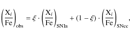
|
(1) |
where
|
(2) |
is the SNIa iron-mass-fraction, i.e. the fraction of the iron mass synthesized in type Ia supernovae,
Matteucci & Chiappini (2005) caution against an inappropriate use of Eq. (1) as in principle this equation is valid only if one is interested in the global Fe production (i.e., Fe in stars, galaxies and the ICM). Indeed, the model leading to Eq. (1) does not consider the finite timescale over which the gas is processed through stars and ignores the mechanism of chemical enrichment of the ICM from galaxies. However, as already noted by de Plaa et al. (2007) and Humphrey & Buote (2006), Eq. (1) can be applied to the ICM, but the iron mass fractions that are derived from it should be interpreted as the iron mass fractions that would be needed to enrich the ICM, not as the actual iron mass fraction produced throughout the history of the cluster.
By inserting Si/Fe and Ni/Fe ratios expected for SNIa and SNcc and the
mean observed Si/Fe and Ni/Fe ratios in Eq. (1) we estimate the SNIa
iron-mass-fraction ![]() .
We compute
.
We compute ![]() by combining several
theoretical SNe yields; the ones for SNIa originate from two
physically different sets of models taken from Iwamoto et al. (1999),
namely the slow deflagration (W7 and W70) and the delayed detonation
(WDDs and CDDs) explosion models. For core-collapsed supernovae we
use the yields from Nomoto et al. (2006), Chieffi & Limongi (2004) and
Woosley & Weaver (1995); details on the models and the computation of the
yields are provided in Appendix A (available online only). Since we
have two equations, one for Si/Fe the other for Ni/Fe, with one
unknown,
by combining several
theoretical SNe yields; the ones for SNIa originate from two
physically different sets of models taken from Iwamoto et al. (1999),
namely the slow deflagration (W7 and W70) and the delayed detonation
(WDDs and CDDs) explosion models. For core-collapsed supernovae we
use the yields from Nomoto et al. (2006), Chieffi & Limongi (2004) and
Woosley & Weaver (1995); details on the models and the computation of the
yields are provided in Appendix A (available online only). Since we
have two equations, one for Si/Fe the other for Ni/Fe, with one
unknown, ![]() ,
we are in a position to determine whether a given
combination of Ia and core-collapsed models can adequately reproduce
the observed ratios. One way of going about this
(e.g. de Plaa et al. 2007) is to perform a
,
we are in a position to determine whether a given
combination of Ia and core-collapsed models can adequately reproduce
the observed ratios. One way of going about this
(e.g. de Plaa et al. 2007) is to perform a ![]() fit using the
observed Si/Fe and Ni/Fe ratios and associated errors as the data, the
Si and Ni yields relative to Fe for SNIa and SNcc, namely
fit using the
observed Si/Fe and Ni/Fe ratios and associated errors as the data, the
Si and Ni yields relative to Fe for SNIa and SNcc, namely
![]() and
and
![]() ,
as constants and
,
as constants and ![]() as
a fitting parameter.
We prefer to proceed differently, as has been noted that the
uncertainties associated with the SNe yields are of the order of tens
of percent (e.g., Woosley & Weaver 1995; Gibson et al. 1997, P. Young priv. comm.,
and the scatter in the yields we have gathered from the literature
fully confirms this, see Table A.1 and Appendix A,
available online only), while our observed mean values of Si/Fe and
Ni/Fe have errors smaller than 5%, if we, for the time being, neglect
the uncertainties associated with the spectral model. Consequently a
robust estimate of
as
a fitting parameter.
We prefer to proceed differently, as has been noted that the
uncertainties associated with the SNe yields are of the order of tens
of percent (e.g., Woosley & Weaver 1995; Gibson et al. 1997, P. Young priv. comm.,
and the scatter in the yields we have gathered from the literature
fully confirms this, see Table A.1 and Appendix A,
available online only), while our observed mean values of Si/Fe and
Ni/Fe have errors smaller than 5%, if we, for the time being, neglect
the uncertainties associated with the spectral model. Consequently a
robust estimate of ![]() should first take into account the
uncertainties in the yields. Given the lack of precise information, we
have assumed a uniform indetermination in the Si and Ni yields
relative to Fe for SNIa and SNcc of 20%. For each combination of
SNIa and SNcc models we allow the Si and Ni yields relative to Fe for
SNIa and SNcc to vary by 20% and, using the observed Si/Fe and Ni/Fe
ratios, we determine the range of values of
should first take into account the
uncertainties in the yields. Given the lack of precise information, we
have assumed a uniform indetermination in the Si and Ni yields
relative to Fe for SNIa and SNcc of 20%. For each combination of
SNIa and SNcc models we allow the Si and Ni yields relative to Fe for
SNIa and SNcc to vary by 20% and, using the observed Si/Fe and Ni/Fe
ratios, we determine the range of values of ![]() for which Eq. (1) is
satisfied. For some combinations of SNIa and SNcc models, despite the
generous 20% range, there are no values of
for which Eq. (1) is
satisfied. For some combinations of SNIa and SNcc models, despite the
generous 20% range, there are no values of ![]() satisfying Eq. (1),
which implies that the observed Si/Fe and Ni/Fe cannot be reproduced
for that particular combination of SNIa and SNcc models.
satisfying Eq. (1),
which implies that the observed Si/Fe and Ni/Fe cannot be reproduced
for that particular combination of SNIa and SNcc models.
In Table 5 (available online only) we report ranges of
values for ![]() for all possible combinations of Ia and
core-collapsed supernovae models. The overall permitted range for
for all possible combinations of Ia and
core-collapsed supernovae models. The overall permitted range for
![]() is large
0.48-0.79 and sensitive to the indetermination in
the SNe yield ratios, indeed assuming 10% or 30% rather than 20% we
derive a range of
0.55-0.73 and
0.37-0.85, respectively.
Since the indetermination in the abundance ratios related to the
emission model is comparable to the one in the yields we recompute the
SNIa iron-mass-fraction assuming abundance ratios derived from apec rather than mekal. The results are similar, see Table A.1, the overall permitted range for
is large
0.48-0.79 and sensitive to the indetermination in
the SNe yield ratios, indeed assuming 10% or 30% rather than 20% we
derive a range of
0.55-0.73 and
0.37-0.85, respectively.
Since the indetermination in the abundance ratios related to the
emission model is comparable to the one in the yields we recompute the
SNIa iron-mass-fraction assuming abundance ratios derived from apec rather than mekal. The results are similar, see Table A.1, the overall permitted range for ![]() is similar
0.49-0.90, the major difference is in which of the combinations of
SNIa and SNcc models provide valid solutions.
is similar
0.49-0.90, the major difference is in which of the combinations of
SNIa and SNcc models provide valid solutions.
Equations (1) and (2) may be generalized to any atomic species and can therefore be used to obtain the Xi elements SNIa gas-mass-fraction. We have done so and derived the Si and Ni SNIa gas-mass-fraction ranges which are respectively 0.14-0.49 and 0.26-0.88.
By adopting abundance ratios derived from apec, we find broader ranges both for Si, 0.12-0.86, and Ni, 0.01-0.90. The reason for this difference rests in the smaller Ni/Fe ratio found with apec. More specifically, the mekal value, 2.41, is relatively high when compared to the Ni/Fe ratios predicted by SNIa and SNcc models. This implies that the observed Ni/Fe and Si/Fe ratios may only be reproduced by a limited combination of SNIa and SNcc models. Conversely, the apec value, 1.88, is closer to the mean Ni/Fe ratio predicted by models and may be reproduced by a broader combination of SNIa and SNcc yields.
The total Fe mass ejected by SNIa,
![]() ,
and by SNcc,
,
and by SNcc,
![]() can be rewritten
as:
can be rewritten
as:
| (3) |
and
| (4) |
where
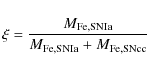
We define
![]() as the
number ratio of supernovae type Ia over the total number of
supernovae; combining Eq. (2) with Eqs. (3) and (4) we solve for f:
as the
number ratio of supernovae type Ia over the total number of
supernovae; combining Eq. (2) with Eqs. (3) and (4) we solve for f:
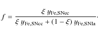
|
(5) |
In Table 6 (available online only) we report estimates for f obtained by inserting allowed ranges for
7 Discussion
In this work we have analyzed the central regions (
![]() )
of a sample of 26 nearby and rich cool core clusters derived
from the original B55 cluster sample (Edge et al. 1990). We have used
these regions characterized by the highest cluster photon statistics
to identify all the possible sources of systematic uncertainties in
the abundance measurements of the most relevant elements observable in
the X-ray spectral range between 1.8 and 10 keV, namely silicon, iron
and nickel.
)
of a sample of 26 nearby and rich cool core clusters derived
from the original B55 cluster sample (Edge et al. 1990). We have used
these regions characterized by the highest cluster photon statistics
to identify all the possible sources of systematic uncertainties in
the abundance measurements of the most relevant elements observable in
the X-ray spectral range between 1.8 and 10 keV, namely silicon, iron
and nickel.
Our analysis shows that, within the cool cores of bright nearby clusters, metal abundances of Si, Fe and in a few instances even Ni can be measured to a high precision. Indeed the precision is so high, particularly for Fe, that we need to introduce a cross-calibration uncertainty of 3% to reconcile measurements secured with different EPIC experiments. Thanks to the high statistical quality of our data, we find evidence for some intrinsic scatter in the element abundance with Fe around 20% and Si and Ni about 30% abundance ratios are also characterized by roughly the same intrinsic scatter.
The relatively modest scatter around mean values of Si, Fe and Ni abundances and Si/Fe and Ni/Fe ratios indicates that, whatever the process responsible for the enrichment of the ICM, it works similarly in all objects. Even in the somewhat extraordinary case of the Centaurus cluster with its anomalously large metal content, the abundances relative to iron are perfectly compatible with those of the other clusters, indicating the presence of similar enrichment processes. Uncertainties in the abundance estimates associated with the specific choice of spectral model, i.e. 2T rather than 4T appear to be negligible (i.e., within the statistical uncertainties for Si and Ni, and of the same order as the EPIC cross-calibration differences for iron).
The estimate of the abundances from our spectra may be thought of, with some simplification, as a two step process: in the first step the equivalent width of a given line is estimated; in the second step the equivalent width is converted into an abundance assuming the temperature derived by fitting the continuum. While the first step is relatively straight-forward and, at least for K-shell lines, leaves little room for ambiguity, the second, requiring estimates of collisional ionization and transition probabilities, is far more prone to differences. We have verified that the two plasma codes available within XSPEC provide somewhat different estimates for the metal abundances; the differences are not huge and are qualitatively similar to those found by other workers (Sanders & Fabian 2006; de Plaa et al. 2007). However, given the high quality of our abundance estimates, they provide the dominant source of indetermination for Si (10%), Ni (16%) and Ni/Fe (22%) and contribute substantially in the case of Fe (4%) and Si/Fe (%6).
We find that the Si/Fe abundance ratio estimated for cool core clusters (this work; Tamura et al. 2004), shows a remarkably good agreement with the values found from samples of galaxy groups (Rasmussen & Ponman 2007) and X-ray luminous elliptical galaxies (Humphrey & Buote 2006). This similarity favors a common enrichment scenario for luminous elliptical galaxies and the cool cores of groups and clusters, i.e. a similar mix of SNIa and SNcc.
We have used our estimates of the Si/Fe and Ni/Fe abundance ratios to constrain the relative contribution of type Ia and core-collapsed supernovae to the enrichment process. To this end we have compiled a list of SNIa and SNcc yields from the literature. Simply by inspecting our yields (see Tables A.1 and A.2 available online only) it is rather obvious that the large differences, in the tens of %, are bound to have a non-negligible impact on our estimates. The Fe normalized yields of Si and Ni both feature a scatter that is larger than the indetermination in the corresponding observed abundance ratios. Under the rather simplistic assumption of a 20% indetermination in the yields we find that, f, the fraction of Ia to Ia plus core-collapsed supernovae cannot be reconciled with 0 or 1, in other words we need both Ia and core-collapsed supernovae to produce the observed ratios. This result appears to be rather solid; an indetermination of at least 50% is required to allow f=0 and then only for one specific combination of Ia and core-collapsed supernovae, an indetermination of more than 70% to have f=1.
Going beyond the qualitative statement that both SNIa and SNcc contribute to the enrichment of the ICM is quite hard. The accepted range for f, the ratio of type Ia SN to all SNe, convolved over all the SNIa and SNcc combinations providing valid results, is rather large, from 10% to 40%. Similarly we can say that roughly more than half (48-79%) of the Fe is produced by SNIa; less than half of the Si (14-49%) is produced by SNIa and Ni is very poorly constrained (26-88%). Increasing the indetermination on the yields beyond 20% will of course further enlarge the allowed ranges and result in even weaker constraints. We reiterate that the limiting factor is not the X-ray abundance estimates, as mean values can be constrained rather well even when allowing for systematics associated with instrument calibration and thermal emission model uncertainties, but rather is the large indetermination in the theoretical yields. A similar point was made some ten years ago by Gibson et al. (1997), a decade later the substantially improved observational constraints stand out in contrast with the lack of any similar advancement on the theoretical side.
Our analysis shows how difficult it is to determine the relative contribution of type Ia and core-collapsed supernovae to the enrichment of the ICM from global cool core measurements. An alternative approach is to measure radial profiles of metal abundances. In this case the variation of an abundance ratio such as Si/Fe, where the two elements are produced in different proportions by SNcc and SNIa, can be interpreted as evidence for a variation of the contribution of one type of SN with respect to the other. This kind of analysis has been attempted in the past, Finoguenov et al. (2000,2001), using ASCA data, found that for most rich clusters in their sample the Si/Fe rapidly increased when moving from small to large radii. Later work using XMM-Newton data did not confirm these findings; Tamura et al. (2004) find a flat Si/Fe ratio for a sample of 19 clusters. Amongst the few objects in common between the ASCA and XMM-Newton samples are A3112 (Finoguenov et al. 2000) and A2052 (Finoguenov et al. 2001) for which ASCA data found Si/Fe radial gradients and XMM-Newton derived flat Si/Fe profiles. Recent analysis of SUZAKU data (Komiyama et al. 2009; Sato et al. 2009b,a,2007b) on a handful of groups and poor clusters leads to Si/Fe profiles that are consistent with being constant out to at least 0.1 r180 and in some instances to 0.2 r180. Since at 0.1 r180 the average Fe abundance excess is about 1/2 of what it is within 0.03 r180(Leccardi & Molendi 2008a), this seems to rule out the possibility that the transition from central excess to flat Fe profile might be associated with a change in SN type mix.
Future work on XMM-Newton, Chandra and SUZAKU data may change the situation somewhat by providing new abundance ratio measurements beyond 0.1 r180. However, given the considerable difficulties involved in estimating abundances at large radii (e.g. Leccardi & Molendi 2008a), it is by no means clear if and by how much our estimates will improve. A major advancement will be provided by the first mission carrying a micro-calorimeter, most likely the Japanese ASTRO-H. The ten fold increase in resolution at the Si line will allow us to reduce the background by an order of magnitude for the H-like Si line and by a factor of a few for the He-like Si triplet. This will translate into measures of Si abundances out to at least 0.3 r180 for a good number of nearby clusters.
8 Summary
We have performed a detailed study of the Si, Fe and Ni abundances in the cores of 26 nearby cool core clusters. Our work may be divided into two main parts; the first relates to the measure of the abundances and the second to the estimate of the relative contribution of SNIa and SNcc to the ICM enrichment process. Regarding the first part, our main result may be summarized as follows.
-
We find that systematic uncertainties associated with the different
spectral modeling, namely a 2T versus 4T model, are below a few per cent
(
 ).
).
-
We find evidence for a
 systematic error between Si and Fe
abundance measures secured with the three EPIC detectors. The Ni
abundances do not have the statistical quality to investigate such
small systematic errors.
systematic error between Si and Fe
abundance measures secured with the three EPIC detectors. The Ni
abundances do not have the statistical quality to investigate such
small systematic errors.
-
We have verified that the mekal and apec plasma codes
available in XSPEC give somewhat different abundances values. Given
the high photon statistics of our spectra, they contribute
significantly to the indetermination of Fe (
 )
and Si/Fe (
)
and Si/Fe ( )
and are the dominant source of indetermination from Si (
)
and are the dominant source of indetermination from Si (
 ),
Ni (
),
Ni ( )
and Ni/Fe (
)
and Ni/Fe ( ).
).
-
The final Si, Fe and Ni abundance distributions as well as the Si/Fe
and Ni/Fe abundance ratio distributions of the sample show only
moderate spreads (from
to
 )
around their mean values
(exact values are reported in Table 4). These nearly
constant distributions suggest similar ICM enrichment processes at
work in all cluster cores.
)
around their mean values
(exact values are reported in Table 4). These nearly
constant distributions suggest similar ICM enrichment processes at
work in all cluster cores.
- We find a remarkable uniformity in the observed Si/Fe abundance ratio ranging from X-ray luminous elliptical galaxies to the cool cores of groups and clusters. This tells us that, whatever the real proportion between different SNe types may be, the enrichment process of the hot gas associated with elliptical galaxies is likely the same in isolated ellipticals, dominant galaxies in groups and the brightest cluster galaxies in clusters.
-
The SNIa iron mass fraction,
 ,
overall permitted range is
0.48-0.79.
,
overall permitted range is
0.48-0.79.
- The SNIa silicon mass fraction and nickel mass fraction ranges are 0.14-0.49 and 0.26-0.88, respectively.
- The number ratio of SNIa over the total number of SNe, f, spans from 0.10 to 0.38.
-
The dominant source of uncertainty in the estimate of
is errors
on theoretical yields; conversely, the choice of spectral code has
almost no impact.
We acknowledge useful discussions with Mariachiara Rossetti and Fabio Gastaldello. This research has made use of the NASA/IPAC Extragalactic Database (NED) which is operated by the Jet Propulsion Laboratory, California Institute of Technology, of the NASA's High Energy Astrophysics Science Archive Research Center (HEASARC), and, of the XMM-Newton archive.
References
- Anders, E., & Grevesse, N. 1989, Geochim. Cosmochim. Acta, 53, 197 [NASA ADS] [CrossRef]
- Arimoto, N., & Yoshii, Y. 1987, A&A, 173, 23 [NASA ADS]
- Arnaud, K. A. 1996, in Astronomical Data Analysis Software and Systems V, ed. G. H. Jacoby, & J. Barnes, ASP Conf. Ser., 101, 17
- Arnaud, M., Rothenflug, R., Boulade, O., Vigroux, L., & Vangioni-Flam, E. 1992, A&A, 254, 49 [NASA ADS]
- Asplund, M., Grevesse, N., & Sauval, A. J. 2005, in Cosmic Abundances as Records of Stellar Evolution and Nucleosynthesis, ed. T. G. Barnes, III, & F. N. Bash, ASP Conf. Ser., 336, 25
- Baumgartner, W. H., Loewenstein, M., Horner, D. J., & Mushotzky, R. F. 2005, ApJ, 620, 680 [NASA ADS] [CrossRef]
- Bland-Hawthorn, J., Veilleux, S., & Cecil, G. 2007, Ap&SS, 311, 87 [NASA ADS] [CrossRef]
- Böhringer, H., Matsushita, K., Churazov, E., Finoguenov, A., & Ikebe, Y. 2004, A&A, 416, L21 [NASA ADS] [EDP Sciences] [CrossRef]
- Chieffi, A., & Limongi, M. 2004, ApJ, 608, 405 [NASA ADS] [CrossRef]
- De Grandi, S., & Molendi, S. 2001, ApJ, 551, 153 [NASA ADS] [CrossRef]
- De Grandi, S., Ettori, S., Longhetti, M., & Molendi, S. 2004, A&A, 419, 7 [NASA ADS] [EDP Sciences] [CrossRef]
- de Plaa, J., Werner, N., Bleeker, J. A. M., et al. 2007, A&A, 465, 345 [NASA ADS] [EDP Sciences] [CrossRef]
- Edge, A. C., Stewart, G. C., Fabian, A. C., & Arnaud, K. A. 1990, MNRAS, 245, 559 [NASA ADS]
- Finoguenov, A., David, L. P., & Ponman, T. J. 2000, ApJ, 544, 188 [NASA ADS] [CrossRef]
- Finoguenov, A., Arnaud, M., & David, L. P. 2001, ApJ, 555, 191 [NASA ADS] [CrossRef]
- Finoguenov, A., Matsushita, K., Böhringer, H., Ikebe, Y., & Arnaud, M. 2002, A&A, 381, 21 [NASA ADS] [EDP Sciences] [CrossRef]
- Fukazawa, Y., Makishima, K., Tamura, T., et al. 1998, PASJ, 50, 187 [NASA ADS]
- Fukazawa, Y., Makishima, K., Tamura, T., et al. 2000, MNRAS, 313, 21 [NASA ADS] [CrossRef]
- Gastaldello, F., & Molendi, S. 2002, ApJ, 572, 160 [NASA ADS] [CrossRef]
- Gibson, B. K., Loewenstein, M., & Mushotzky, R. F. 1997, MNRAS, 290, 623 [NASA ADS]
- Grevesse, N., & Sauval, A. J. 1998, Space Sci. Rev., 85, 161 [NASA ADS] [CrossRef]
- Humphrey, P. J., & Buote, D. A. 2006, ApJ, 639, 136 [NASA ADS] [CrossRef]
- Ishimaru, Y., & Arimoto, N. 1997, PASJ, 49, 1 [NASA ADS]
- Iwamoto, K., Brachwitz, F., Nomoto, K., et al. 1999, ApJS, 125, 439 [NASA ADS] [CrossRef]
- Kaastra, J. S., Paerels, F. B. S., Durret, F., Schindler, S., & Richter, P. 2008, Space Sci. Rev., 134, 155 [NASA ADS] [CrossRef]
- Kalberla, P. M. W., Burton, W. B., Hartmann, D., et al. 2005, A&A, 440, 775 [NASA ADS] [EDP Sciences] [CrossRef]
- Komiyama, M., Sato, K., Nagino, R., Ohashi, T., & Matsushita, K. 2009, PASJ, 61, 337
- Leccardi, A., & Molendi, S. 2008a, A&A, 487, 461 [NASA ADS] [EDP Sciences] [CrossRef]
- Leccardi, A., & Molendi, S. 2008b, A&A, 486, 359 [NASA ADS] [EDP Sciences] [CrossRef]
- Leccardi, A., Rossetti, M. C., & Molendi, S. 2009, A&A, submitted
- Lodders, K. 2003, ApJ, 591, 1220 [NASA ADS] [CrossRef]
- Maccacaro, T., Gioia, I. M., Wolter, A., Zamorani, G., & Stocke, J. T. 1988, ApJ, 326, 680 [NASA ADS] [CrossRef]
- Mannucci, F., Della Valle, M., & Panagia, N. 2006, MNRAS, 370, 773 [NASA ADS]
- Matsushita, K., & Suzaku SWG team. 2008, Astron. Nachr., 329, 139 [NASA ADS] [CrossRef]
- Matteucci, F., & Chiappini, C. 2005, PASA, 22, 49 [NASA ADS]
- Molendi, S., & Gastaldello, F. 2009, A&A, 493, 13 [NASA ADS] [EDP Sciences] [CrossRef]
- Ness, J. U., Ehle, M., Gonzalez Riestra, R., et al. 2009, XMM-Newton Users' Handbook, http://xmm.esac.esa.int./external/xmm_user_suport/documentation/uhb/index.html
- Nomoto, K., Tominaga, N., Umeda, H., Kobayashi, C., & Maeda, K. 2006, Nuclear Phys. A, 777, 424 [NASA ADS] [CrossRef]
- Peres, C. B., Fabian, A. C., Edge, A. C., et al. 1998, MNRAS, 298, 416 [NASA ADS] [CrossRef]
- Rasmussen, J., & Ponman, T. J. 2007, MNRAS, 380, 1554 [NASA ADS] [CrossRef]
- Renzini, A., Ciotti, L., D'Ercole, A., & Pellegrini, S. 1993, ApJ, 419, 52 [NASA ADS] [CrossRef]
- Salpeter, E. E. 1955, ApJ, 121, 161 [NASA ADS] [CrossRef]
- Sanders, J. S., & Fabian, A. C. 2006, MNRAS, 371, 1483 [NASA ADS] [CrossRef]
- Sato, K., Tokoi, K., Matsushita, K., et al. 2007a, ApJ, 667, L41 [NASA ADS] [CrossRef]
- Sato, K., Yamasaki, N. Y., Ishida, M., et al. 2007b, PASJ, 59, 299 [NASA ADS]
- Sato, K., Matsushita, K., & Gastaldello, F. 2009a, PASJ, 61, 365
- Sato, K., Matsushita, K., Ishisaki, Y., et al. 2009b, PASJ, 61, 353
- Schindler, S., & Diaferio, A. 2008, Space Sci. Rev., 134, 363 [NASA ADS] [CrossRef]
- Scott, P., Asplund, M., Grevesse, N., & Sauval, A. J. 2009, ApJ, 691, L119 [NASA ADS] [CrossRef]
- Smith, R. K., Brickhouse, N. S., Liedahl, D. A., & Raymond, J. C. 2001, ApJ, 556, L91 [NASA ADS] [CrossRef]
- Tamura, T., Kaastra, J. S., den Herder, J. W. A., Bleeker, J. A. M., & Peterson, J. R. 2004, A&A, 420, 135 [NASA ADS] [EDP Sciences] [CrossRef]
- Werner, N., Durret, F., Ohashi, T., Schindler, S., & Wiersma, R. P. C. 2008, Space Sci. Rev., 134, 337 [NASA ADS] [CrossRef]
- Woosley, S. E., & Weaver, T. A. 1995, ApJS, 101, 181 [NASA ADS] [CrossRef]
- Young, P. A., & Fryer, C. L. 2007, ApJ, 664, 1033 [NASA ADS] [CrossRef]
Online Material
Appendix A:
We have computed yields for Si, Fe and Ni for different models of Ia and core-collapsed supernovae.
The ones for SNIa originate from two physically distinct sets of models taken from Iwamoto et al. (1999), namely the slow deflagration (W7 and W70) and the delayed detonation (WDDs and CDDs) explosion models. We have computed silicon, iron and nickel yields for a given SNIa model by summing over all stable isotopes the synthesized amount of Si, Fe and Ni per SN event given in Table A.1 of Iwamoto et al. (1999).
For core-collapsed supernovae we use the yields from Nomoto et al. (2006),
Chieffi & Limongi (2004) and Woosley & Weaver (1995).
In these cases we first averaged the yields over the initial mass
function (IMF) of the stellar population as follows:
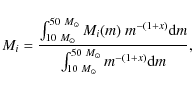
|
(A.1) |
where Mi(m) is the ith element mass produced by a star of mass m. We consider two IMF: a standard Salpeter (1955) function with exponent x=1.35, and a top-heavy function with x=0.95(Arimoto & Yoshii 1987, thereafter AY), which predicts a relatively larger number of massive stars. The integration mass range is between 10 and 50 solar masses, in agreement with Nomoto et al. (2006).
Table A.1: Yields of elements in solar masses for different SNe models. Type Ia yields were calculated for each element for the W7, W70, WDD1, WDD2, WDD3 and CDD1, CDD2 models in Iwamoto et al. (1999). SN core-collapsed yields (including types Ib and Ic) were calculated from the results in Nomoto et al. (2006) integrating over a progenitor initial mass function. We have considered two different initial mass functions, the Salpeter function with index 1.35 and the AY top-heavy function with index 0.95, and we have integrated between 10 and 50 solar masses. The initial metallicity of the progenitors is Z=0.02 (i.e. solar).
Table A.2: Yields of Si and Ni relative to Fe in solar units of Anders & Grevesse (1989) for the same SNe models used in Table A.1.
The derived yields of Si, Fe and Ni in units of solar masses per supernova explosion are reported in Table A.1. For core-collapsed supernovae we report results for the standard Salpeter and the AY top-heavy IMF.
Inspection of Table A.1 reveals how much yields differ from one model to the other. Fe is characterized by the smallest scatter, 10% for SNIa and 18% for SNcc, Si is less constrained, 27% for SNIa and 19% for SNcc, Ni features the largest variations, 46% for SNIa and 41% for SNcc. Note also that the choice of IMF produces only a modest impact on the yields.
The derived SNIa yields of Si and Ni relative to iron in Anders & Grevesse (1989) solar units are reported in Table A.2. Ratios in Grevesse & Sauval (1998) units can be easily computed by multiplying both the Si/Fe and Ni/Fe values in Table A.2 by 0.675, whereas ratios in Lodders (2003) units are obtained by multiplying Si/Fe by 0.65 and Ni/Fe by 0.68, and, ratios in Asplund et al. (2005) units by multiplying Si/Fe by 0.67 and Ni/Fe by 0.72 (for the solar Ni we have used the updated value by Scott et al. 2009).
The derived yields of Si and Ni relative to iron in solar units for SNcc for different progenitor metallicities and IMFs are reported in Table A.2. Conversion factors for different solar units systems are the same as given above.
The yields relative to Fe for all our SNcc models are also listed in a recent review paper (Werner et al. 2008). Unfortunately some of the values reported in that paper are incorrect, in some cases, by a large amount, i.e. the Ni yields for the Woosley & Weaver (1995) models. We have corresponded with the authors who are now considering publishing a revised version of their tables.
Table 1: Starting sample of 32 galaxy clusters extracted from the X-ray flux limited B55 sample (Edge et al. 1990).
Table 2: Relative differences between metal measurements made with the three EPIC instruments MOS1, MOS2 and pn computed over the whole sample.
Table 3: Measurements of silicon, iron and nickel abundances relative to the solar value (Anders & Grevesse 1989) for the final sample (26 clusters for Si and Fe, 23 for Ni) from the 4T mekal spectral model.
Table 4: Averages of Si, Fe, Ni abundances and Si/Fe, Ni/Fe ratios for the cool core cluster sample in solar units.
Table 5:
Supernovae type Ia mass fraction,
![]() ,
obtained for different
theoretical SNe silicon-to-iron and nickel-to-iron ratios from the
observed Si/Fe and Ni/Fe ratios.
,
obtained for different
theoretical SNe silicon-to-iron and nickel-to-iron ratios from the
observed Si/Fe and Ni/Fe ratios.
Table 6:
Supernovae type Ia fraction,
![]() ,
obtained for different theoretical SNe models from the observed Si/Fe
and Ni/Fe abundance ratios. SNIa and SNcc models are the same as in
Table 5.
,
obtained for different theoretical SNe models from the observed Si/Fe
and Ni/Fe abundance ratios. SNIa and SNcc models are the same as in
Table 5.
Footnotes
- ... clusters
- Tables and Appendix are only available in electronic form at http://www.aanda.org
All Tables
Table A.1: Yields of elements in solar masses for different SNe models. Type Ia yields were calculated for each element for the W7, W70, WDD1, WDD2, WDD3 and CDD1, CDD2 models in Iwamoto et al. (1999). SN core-collapsed yields (including types Ib and Ic) were calculated from the results in Nomoto et al. (2006) integrating over a progenitor initial mass function. We have considered two different initial mass functions, the Salpeter function with index 1.35 and the AY top-heavy function with index 0.95, and we have integrated between 10 and 50 solar masses. The initial metallicity of the progenitors is Z=0.02 (i.e. solar).
Table A.2: Yields of Si and Ni relative to Fe in solar units of Anders & Grevesse (1989) for the same SNe models used in Table A.1.
Table 1: Starting sample of 32 galaxy clusters extracted from the X-ray flux limited B55 sample (Edge et al. 1990).
Table 2: Relative differences between metal measurements made with the three EPIC instruments MOS1, MOS2 and pn computed over the whole sample.
Table 3: Measurements of silicon, iron and nickel abundances relative to the solar value (Anders & Grevesse 1989) for the final sample (26 clusters for Si and Fe, 23 for Ni) from the 4T mekal spectral model.
Table 4: Averages of Si, Fe, Ni abundances and Si/Fe, Ni/Fe ratios for the cool core cluster sample in solar units.
Table 5:
Supernovae type Ia mass fraction,
![]() ,
obtained for different
theoretical SNe silicon-to-iron and nickel-to-iron ratios from the
observed Si/Fe and Ni/Fe ratios.
,
obtained for different
theoretical SNe silicon-to-iron and nickel-to-iron ratios from the
observed Si/Fe and Ni/Fe ratios.
Table 6:
Supernovae type Ia fraction,
![]() ,
obtained for different theoretical SNe models from the observed Si/Fe
and Ni/Fe abundance ratios. SNIa and SNcc models are the same as in
Table 5.
,
obtained for different theoretical SNe models from the observed Si/Fe
and Ni/Fe abundance ratios. SNIa and SNcc models are the same as in
Table 5.
All Figures
|
|
Figure 1: EPIC- pn spectral data (crosses) and best-fit models (continuum lines) for 3 high counting statistics clusters: Perseus (on the top), 2A 0335+096 (in the middle) and Centaurus (at the bottom). Panels on the left show results from a 4T model fit without Gaussian smoothing whereas plots on the right are smoothed. In all cases we also plot the data divided by the folded model. The spectra are rebinned for clarity. The energy range of each plot is 600 eV centered on the 6.7 keV line (redshifted at the cluster distance). In the panels on the left the ``wings'' around the Fe line are clearly visible in the residuals, an indication of the resolution mis-calibration of the redistribution matrix of the pn (see discussion in Sect. 4.1). |
| Open with DEXTER | |
| In the text | |
|
|
Figure 2:
Silicon ( upper panel), iron ( medium panel) and nickel
( lower panel) abundances measured in the core region with r < 0.5
|
| Open with DEXTER | |
| In the text | |
|
|
Figure 3: Silicon-to-iron ( upper panel) and nickel-to-iron ( lower panel) ratios for the cluster sample. |
| Open with DEXTER | |
| In the text | |
Copyright ESO 2009
Current usage metrics show cumulative count of Article Views (full-text article views including HTML views, PDF and ePub downloads, according to the available data) and Abstracts Views on Vision4Press platform.
Data correspond to usage on the plateform after 2015. The current usage metrics is available 48-96 hours after online publication and is updated daily on week days.
Initial download of the metrics may take a while.