| Issue |
A&A
Volume 508, Number 1, December II 2009
|
|
|---|---|---|
| Page(s) | 513 - 524 | |
| Section | Atomic, molecular, and nuclear data | |
| DOI | https://doi.org/10.1051/0004-6361/200912557 | |
| Published online | 08 October 2009 | |
A&A 508, 513-524 (2009)
Benchmarking atomic data for astrophysics: Fe VIII EUV lines
G. Del Zanna
DAMTP, Centre for Mathematical Sciences, Wilberforce road, Cambridge CB3 0WA, UK
Received 22 May 2009 / Accepted 17 September 2009
Abstract
The EUV spectrum of
Fe VIII is reviewed, using new solar observations from the
Hinode EUV Imaging Spectrometer (EIS), together with older solar and laboratory data.
The most up-to-date scattering calculations
are benchmarked against these
experimental data,
with the use of a large atomic structure calculation.
Once adjustments are made to the excitation rates,
good agreement is found between calculated and observed
line intensities.
All previous line identifications have been re-assessed.
Several lines are identified here for the first time, most notably
the strong decays from the 3s2 3p5 3d2 4Dj levels.
It is shown that they provide a new, important diagnostic of electron temperature
for the upper transition region.
The temperatures obtained at the base of solar coronal loops
are lower (log T [K] = 5.5) than those predicted by assuming ionization
equilibrium (log T [K] = 5.6), however firm measurements
will only be possible once better scattering calculations
are available, and the EIS radiometric calibration is
properly assessed.
Key words: line: identification - atomic data - Sun: transition region - techniques: spectroscopic
1 Introduction
This paper is one of a series in which atomic data and line identifications are benchmarked against experimental data. The method and goals are described in Del Zanna et al. (2004), where Fe X was discussed. New solar observations from the Hinode EUV Imaging Spectrometer (EIS, see Culhane et al. 2007) have shown the presence of a wealth of spectral lines formed at transition region (hereafter TR) temperatures (Young et al. 2007), and offer the opportunity to benchmark atomic data for a variety of ions. The brightest TR lines in the EIS spectra are from Fe VIII, which are assessed in this paper. The assessment of Fe VII and in general of lines formed at similar temperatures is considered in a separate paper (Del Zanna 2009). The Hinode EIS observations are complemented with measurements found in the literature, and with a few new measurements from a plate (Fawcett, priv. comm.). Only EUV transitions (decays from n=3,4 levels) are considered here.
Contrary to many other ions, very little experimental work has been done on Fe VIII EUV lines. The identification of Fe VIII EUV lines started with Kruger & Weissberg (1937)[hereafter KW37], who correctly identified only two of the transitions considered here. Six of the strongest EUV transitions were identified through to the fundamental laboratory work of Fawcett and co-workers on the Zeta spectrum (see Gabriel et al. 1965, hereafter G65). The main source of accurate wavelengths and the identifications of most of the strongest EUV lines came from the excellent work of Ramonas & Ryabtsev (1980) (hereafter RR80). For this benchmark, we consider the most up-to-date electron scattering calculation for this ion by Griffin et al. (2000) (hereafter G00). For a description of previous work on electron impact excitation see G00.
2 Benchmark method and atomic structure calculations
As described in Del Zanna et al. (2004), the benchmark
method starts with an assessment of the observed wavelengths
![]() from
which a set of experimental level energies
from
which a set of experimental level energies
![]() is obtained.
As an aid to the identification process, atomic structure calculations
are run, trying to find a set of ab-initio energies to match the
experimental ones.
To improve the level energies, term energy
corrections (TEC) (see, e.g. Zeippen et al. 1977; Nussbaumer & Storey 1978)
to the LS Hamiltonian matrix are applied, using an
iterative procedure, where first-guess corrections to the LS term energies
are estimated from the
weighted mean of the observed level energies, whenever available.
A large ``benchmark'' basis is normally sought, and the results in terms
of level energy and oscillator strengths compared to those from the scattering
calculation, to assess the validity of the scattering
target.
Once a good match between experimental and theoretical energies is found,
line intensities are calculated by solving the level balance equations in
steady state, and all the strongest spectral lines
(observed or not) are examined in detail.
Observed line intensities
is obtained.
As an aid to the identification process, atomic structure calculations
are run, trying to find a set of ab-initio energies to match the
experimental ones.
To improve the level energies, term energy
corrections (TEC) (see, e.g. Zeippen et al. 1977; Nussbaumer & Storey 1978)
to the LS Hamiltonian matrix are applied, using an
iterative procedure, where first-guess corrections to the LS term energies
are estimated from the
weighted mean of the observed level energies, whenever available.
A large ``benchmark'' basis is normally sought, and the results in terms
of level energy and oscillator strengths compared to those from the scattering
calculation, to assess the validity of the scattering
target.
Once a good match between experimental and theoretical energies is found,
line intensities are calculated by solving the level balance equations in
steady state, and all the strongest spectral lines
(observed or not) are examined in detail.
Observed line intensities
![]() ,
whenever available, are compared to the
theoretical ones by plotting the ``emissivity ratio''
,
whenever available, are compared to the
theoretical ones by plotting the ``emissivity ratio''
|
(1) |
for each line as a function of the electron temperature
It is notoriously difficult to obtain ab-initio level energies that match the observed ones for this ion. Configuration-interaction (CI) effects are very large. For the same reason, it is very difficult to obtain firm identifications for all the strongest lines. Relativistic multi-reference many-body perturbation theory calculations such as those described in Ishikawa & Vilkas (2008) are needed, since they have been proved to provide very good level energies.
Table 1: Electron configuration basis for the benchmark calculation (23C) and orbital scaling parameters.
Table 2: Level energies for Fe VIII.
Table 3: List of strongest Fe VIII lines in the 100-500 Å range.
The G00 scattering target included 33 LS terms from the seven configurations: 3s2 3p6 3d, 3s2 3p5 3d2, 3s2 3p5 3d 4s 3s2 3p6 4s, 3s2 3p6 4p, 3s2 3p6 4d, 3s2 3p6 4f, which are the most important ones for UV and EUV lines. For the radiative rates of a few important transitions, G00 performed a larger CI structure calculation by including terms from the 3s2 3p4 3d3, 3s2 3p3 3d4, 3s2 3p4 3d2 4f configurations, which mix strongly with the 3s2 3p6 3d, 3s2 3p5 3d2, 3s2 3p6 4f. As clearly shown in their Table 2, the radiative rates for strong dipole-allowed transitions reached 30% differences with the values obtained from the target used for the scattering calculation. This implies that the collisions strengths are likely to be incorrect by the same amount. The combined effect of collisions strength (which changes the population of the upper level) and of the transition probability therefore becomes significant.
Zeng et al. (2003) (hereafter Z03) performed large-scale multi-configuration Hartree-Fock (MCHF) calculations for Fe VIII, to show the importance of including core-valence electron correlations. In their case D (which included correlations of the type 3p3-3d3), convergence in the oscillator strengths was achieved, however their level energies were not very accurate.
A ``benchmark'' configuration basis was sought, to obtain a good set of oscillator strengths and level energies. After a large number of tests, the set of 23 configurations listed in Table 1 was chosen. The AUTOSTRUCTURE code (Badnell 1997) was used. Radial scaling parameters were chosen by minimizing the equally-weighted sum of the energies of the LS terms providing the lowest configurations considered here. n=5 correlation orbitals were included. To further improve the energies, term energy corrections (TEC) to the LS Hamiltonian matrix were applied.
The energies of the benchmark calculation (
![]() )
are in
good agreement with the experimental ones (
)
are in
good agreement with the experimental ones (
![]() ), in particular in terms of relative energies
for strongly-mixed levels, as shown in Table 2.
The levels for which it proved most difficult to obtain accurate
energies were:
a) the 3s2 3p5 3d2 2P3/2 (41) which mixes strongly
with 3s2 3p6 4p 2P3/2 (43) and 3s2 3p5 3d2 2P3/2(48); b) 3s2 3p6 4p 2P3/2 (43); c)
3s2 3p5 3d2 2P1/2 (44) which mixes
strongly with the 3s2 3p5 3d2 2P1/2 (47)
and 3s2 3p5 3d2 2P1/2 (23).
The energies from the G00 scattering target (
), in particular in terms of relative energies
for strongly-mixed levels, as shown in Table 2.
The levels for which it proved most difficult to obtain accurate
energies were:
a) the 3s2 3p5 3d2 2P3/2 (41) which mixes strongly
with 3s2 3p6 4p 2P3/2 (43) and 3s2 3p5 3d2 2P3/2(48); b) 3s2 3p6 4p 2P3/2 (43); c)
3s2 3p5 3d2 2P1/2 (44) which mixes
strongly with the 3s2 3p5 3d2 2P1/2 (47)
and 3s2 3p5 3d2 2P1/2 (23).
The energies from the G00 scattering target (
![]() )
and those from Z03 (case D) are also shown in Table 2.
Notice that most
)
and those from Z03 (case D) are also shown in Table 2.
Notice that most
![]() values are accurate, but those from Z03 are not.
values are accurate, but those from Z03 are not.
Table 3 lists the weighted oscillator strengths (gf) for the strongest dipole-allowed transitions, compared to the G00 and Z03 values. The G00 gf values were obtained from the published A-values and the experimental energies, following G00. The 30% differences in the gf values of some of the strongest transitions discussed by G00 are confirmed, however larger differences are present for weaker transitions. The few published gf values from Z03 are in overall agreement with those of the benchmark calculation.
The differences in the gf values imply that the G00 collision strengths at higher temperatures for various transitions are likely to be incorrect by similar amounts. It is well known that the main contribution for strong dipole-allowed transitions comes from high partial waves, where the collision strength is approximately proportional to the gf value for the transition. For the purpose of this paper, it is useful to scale the G00 collision strengths using the benchmark calculation, to see how the resulting line intensities compare with the observed ones. Flower & Nussbaumer (1974) were among the first to suggest scaling collision strengths according to gf (and energy) values, something which has been adopted in many cases within the CHIANTI database (e.g. for Fe X and Fe XI). The scaling has been found to improve agreement between observed and predicted intensities.
The energies and gf values were used to obtain the high-temperature limits in the scaled domain following Burgess & Tully (1992). An example is shown in Fig. 1 (bottom plot), where the scaled collision strengths for the 2-46 transition (dashed line, constant equal to 1.5) and its high-temperature limit are plotted. Good agreement between the G00 collision strengths and the high-temperature limits was found for all lines. The high-temperature limit for the 2-46 transition obtained from the benchmark calculation is however smaller by a factor of 0.7, and is shown in Fig. 1 (bottom plot, scaled temperature = 1). The collision strengths need to be scaled (continuous line) by this factor to converge to this limit, as shown in the Figure. The ratios between the limit values obtained from the benchmark calculation and those obtained from the G00 data were used to scale the thermally-averaged collision strengths for all the dipole-allowed transitions.
Line intensities were calculated with the scaled rates and
the transition probabilities from the benchmark + TEC calculation,
assuming plasma equilibrium conditions, at the
temperature of peak ion abundance for Fe VIII in
ionization equilibrium (log T[K] = 5.6), according to the latest
ionization and recombination rates published within
CHIANTI![]() v.6 (Dere et al. 2009,1997).
These line intensities are listed in Table 3, in decreasing order.
As usual within the benchmark process, all the identifications
of the strongest lines have been checked, using laboratory and solar spectra,
as described in the following section.
Line intensities, whenever available, were compared, in order to
confirm identifications and assess the possible presence of blending.
The results are also shown in Table 3.
Line intensities were also computed adopting the original G00
collision strengths and A-values, with the addition of
v.6 (Dere et al. 2009,1997).
These line intensities are listed in Table 3, in decreasing order.
As usual within the benchmark process, all the identifications
of the strongest lines have been checked, using laboratory and solar spectra,
as described in the following section.
Line intensities, whenever available, were compared, in order to
confirm identifications and assess the possible presence of blending.
The results are also shown in Table 3.
Line intensities were also computed adopting the original G00
collision strengths and A-values, with the addition of
![]() ,
a value calculated with the benchmark target
and in close agreement with the NIST database
,
a value calculated with the benchmark target
and in close agreement with the NIST database![]() value of
value of
![]() .
.
![\begin{figure}
\par\includegraphics[width=8.0cm]{H12557_f1.eps}
\end{figure}](/articles/aa/full_html/2009/46/aa12557-09/img171.png)
|
Figure 1: Top: thermally-averaged collisions strengths for the 2-46 transition. The dashed line indicates the original calculated values from G00, while the continuous one the scaled values (see text). Bottom: the same points, plotted in the scaled domain (Burgess & Tully 1992), with the high-temperature limits (scaled temperature = 1). |
| Open with DEXTER | |
3 Experimental data
The few spectral observations considered here for the benchmark are now described.
3.1 Hinode/EIS
The Hinode/EIS instrument covers
two wavelength bands (SW: 166-212 Å; LW: 245-291 Å
approximately).
This spectral range is crowded with emission lines, and most
spectral lines are significantly blended.
The entire EIS database of observations was searched to find
suitable observations to benchmark this ion.
None was found,
however an observation which was originally analysed for
other purposes is presented
here. It consists of a long-duration raster where the 1
![]() slit
was moved (from west to east, between 2007 Jan. 5 21:52 UT and
2007 Jan. 6 01:07 UT) over a Sunspot while it was
close to Sun centre. The exposure times were long (90 s)
which allowed a good signal even in the weaker lines.
slit
was moved (from west to east, between 2007 Jan. 5 21:52 UT and
2007 Jan. 6 01:07 UT) over a Sunspot while it was
close to Sun centre. The exposure times were long (90 s)
which allowed a good signal even in the weaker lines.
The observation is ideal in the sense that contamination from coronal lines is at a minimum, and Sunspot loops had prominent Fe VIII lines. The drawback of this observation was the small field of view, which considerably limits wavelength measurements. The data analysis to obtain line intensities is quite straightforward, but obtaining accurate wavelengths is quite complex.
As described in Del Zanna (2008a), the main problems in the
analysis of EIS data are the strong (75 km s-1) orbital variation of the
wavelength scale and the offsets in both N-S (18
![]() )
and E-W (2
)
and E-W (2
![]() )
directions between the two channels. The offset in the E-W direction means that observations
in the two channels were not simultaneous nor co-spatial.
During the course of benchmarking Fe XVII, it was also found that
the spectra are slanted relative to the axes of the CCD
by 3.66(
)
directions between the two channels. The offset in the E-W direction means that observations
in the two channels were not simultaneous nor co-spatial.
During the course of benchmarking Fe XVII, it was also found that
the spectra are slanted relative to the axes of the CCD
by 3.66(![]() 0.2) pixels end-to-end (each pixel along the slit corresponds to 1
0.2) pixels end-to-end (each pixel along the slit corresponds to 1
![]() ).
A small tilt is also present.
).
A small tilt is also present.
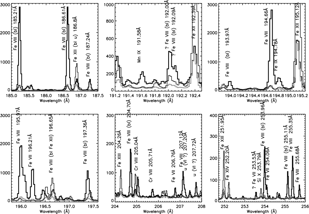
The spectra have been rotated and shifted to take into account the slant and the various misalignments. Two orbital-dependent wavelength calibrations (one for each channel) was obtained, and the spectral tilt included. These wavelengths were used, together with the cfit package (Haugan 1997) to fit Gaussian profiles to the brightest EIS lines. More than 200 lines were fitted and their morphology examined in detail, one by one. Figure 2 shows the resulting monochromatic images for a selection of Fe VIII lines, while Fig. 3 presents images in other lines, to show how sensitive morphology is to temperature (and to a lesser extent to density). This allows us to estimate the temperature of formation for unidentified lines, and to assess if Fe VIII lines are blended. For example, the 193.97 Å line is obviously blended with a hot line formed at temperatures close to that of Fe XVI 269.98 Å (cf. the similarities in the images in Figs. 2, 3).
![\begin{figure}
\par {\includegraphics[width=16.cm]{H12557_f2a.eps} }
{\includegraphics[width=16.cm]{H12557_f2b.eps} }\end{figure}](/articles/aa/full_html/2009/46/aa12557-09/img173.png)
|
Figure 2: Monochromatic images (negative) of the Fe VIII identified lines observed by EIS. Notice that all the Fe VIII lines have a similar morphology. |
| Open with DEXTER | |
![\begin{figure}
{\includegraphics[width=16.cm]{H12557_f3.eps} }\end{figure}](/articles/aa/full_html/2009/46/aa12557-09/img174.png)
|
Figure 3: Monochromatic images (negative) of a selection of EIS lines (ion and wavelength in Å are indicated together with the logarithm of the temperature (K) of formation of the lines in collisional ionization equilibrium). Notice the large morphological differences in lines formed at different temperatures. |
| Open with DEXTER | |
|
Figure 4: Hinode EIS spectra (units are average counts per pixel) over three different areas. Thick lines refer to the spectrum over the Sunspot leg, where Fe VIII lines were clearly strong. The thick grey line shows the foreground Sunspot spectrum, while the thin black spectrum is from the reference area used for the wavelength calibration. |
| Open with DEXTER | |
Figure 5 shows an enlarged portion of the
radiances of two lines recorded in the two EIS channels,
showing agreement to within 1
![]() in the spatial alignment.
This confirms that the geometrical corrections applied here
are accurate.
A region in a Sunspot loop leg, indicated by the crossing
of the two sets of dashed lines in
Fig. 5, was chosen to obtain an
average spectrum to benchmark the Fe VIII lines.
Portions of the spectrum where
Fe VIII lines are present are shown in Fig. 4.
In this spectrum, all TR lines are very strong.
To account for the (small) contribution from the foreground
emission in coronal lines, a nearby foreground spectrum
was obtained, centred on the Sunspot, i.e. where
TR and coronal lines are weak. Portions of this spectrum
are also shown in Fig. 4.
Notice that the strongest EIS coronal line, due to
Fe XII (a self-blend at 195.12 Å
identified by Del Zanna & Mason 2005),
is very weak in the Sunspot spectrum. Moreover,
that its ``foreground'' intensity is almost the
same as that of the Sunspot loop leg. This means
that the ``foreground-subtracted'' Sunspot loop leg spectrum
is virtually free from coronal emission.
This spectrum was used for the benchmark.
in the spatial alignment.
This confirms that the geometrical corrections applied here
are accurate.
A region in a Sunspot loop leg, indicated by the crossing
of the two sets of dashed lines in
Fig. 5, was chosen to obtain an
average spectrum to benchmark the Fe VIII lines.
Portions of the spectrum where
Fe VIII lines are present are shown in Fig. 4.
In this spectrum, all TR lines are very strong.
To account for the (small) contribution from the foreground
emission in coronal lines, a nearby foreground spectrum
was obtained, centred on the Sunspot, i.e. where
TR and coronal lines are weak. Portions of this spectrum
are also shown in Fig. 4.
Notice that the strongest EIS coronal line, due to
Fe XII (a self-blend at 195.12 Å
identified by Del Zanna & Mason 2005),
is very weak in the Sunspot spectrum. Moreover,
that its ``foreground'' intensity is almost the
same as that of the Sunspot loop leg. This means
that the ``foreground-subtracted'' Sunspot loop leg spectrum
is virtually free from coronal emission.
This spectrum was used for the benchmark.
![\begin{figure}
\par\includegraphics[width=8.2cm]{H12557_f5.eps}
\end{figure}](/articles/aa/full_html/2009/46/aa12557-09/img176.png)
|
Figure 5:
Enlarged portion of the Fe VIII 186.60 Å radiance
(negative image, SW channel),
with contours of the Si VII 275.35 Å intensity (LW channel), showing
agreement to within 1
|
| Open with DEXTER | |
![\begin{figure}
\par\includegraphics[width=7.0cm]{H12557_f6a.eps}\par\includegraphics[width=7.0cm]{H12557_f6b.eps}
\end{figure}](/articles/aa/full_html/2009/46/aa12557-09/img177.png)
|
Figure 6: Top: Doppler-gram of the Si VII 275.35 Å line showing strong (20 km s-1 or more) red-shifts in the legs of the coronal loops. The location of the area chosen to obtain averaged spectra from a Sunspot loop leg is indicated by the crossing of the two sets of dashed lines. Bottom: a slice along the N-S dashed lines of the Doppler-shifts in two lines in the SW and LW channels. Despite the lack of simultaneity between the channels, good agreement is found. The dashed lines indicate the location of the chosen Sunspot loop leg area (having a red-shift of about 20 km s-1). |
| Open with DEXTER | |
![\begin{figure}
\par\includegraphics[width=7.0cm]{H12557_f7a.eps}\par\includegraphics[width=7.0cm]{H12557_f7b.eps}
\end{figure}](/articles/aa/full_html/2009/46/aa12557-09/img178.png)
|
Figure 7: Difference between fitted and theoretical wavelengths (Å) in the SW and LW channels of EIS. A linear dispersion for the SW channel was used, while a quadratic one was adopted for the LW. |
| Open with DEXTER | |
Another spectrum was needed for the wavelength calibration. The one chosen is also shown in Fig. 4. The EIS instrument does not have a reference wavelength scale so ideally one would use the spectra of a ``reference'' region to obtain the rest wavelengths. Unfortunately, as shown in Del Zanna (2007,2008b), active regions present Doppler-shifts at all locations in all lines, in particular at TR temperatures, where Fe VIII is formed. This is clearly shown in Fig. 6. The Sunspot leg area selected presents a red-shift of about 20 km s-1 in all TR lines observed in both channels. To obtain good rest wavelengths, a large field of view would be needed, something that was not available. The shifts in the spectra due to thermal effects caused by the satellite orbit are difficult to correct accurately because they are usually wavelength dependent. A reference region was chosen so that it was observed at the same time as the loop leg region (i.e. the same wavelength calibration would apply) at coordinates Solar Y= -84:-64 (see Fig. 6).
Table 4: List of measured wavelengths.
The average reference spectra were calibrated in wavelength, using a set of about 30 lines in each channel. The spectral dispersion is such that the EIS wavelengths vary almost linearly with the CCD pixels. An EIS linear wavelength calibration was used for the SW channel, while a quadratic one was used for the LW. Results are shown in Fig. 7. Theoretical wavelengths from version 5.2 of the CHIANTI atomic package (Landi et al. 2006) were used. These in turn rely mainly on the Behring et al. (1976) full-Sun grazing incidence rocket spectrum and various laboratory data, publised in a series of papers by Fawcett. It is well known that such theoretical wavelengths need to be improved, and indeed such improved reference data are one of the intended by-products of the on-going benchmark work. Overall, as Fig. 7 shows, agreement between the EIS and the reference wavelengths is however accurate to within 6 mÅ across the entire spectral range.
The same wavelength calibration was applied to the ``foreground-corrected'' Sunspot loop leg spectrum, and all the measured wavelengths of TR lines formed at the Fe VIII temperatures were corrected for a red-shift of 20 km s-1. The results are shown in Table 4, together with wavelength measurements from the literature and identifications (a full list is provided in Del Zanna 2009). An overall conservative uncertainty of 10 mÅ is suggested for the measured wavelengths. Note, however, that despite the lack of an appropriate reference spectrum, the measured wavelengths are well within this uncertainty for the previously-known Fe VIII, Si VI, Mg VI, Mg VI lines, while they differ significantly for Si VII. It is likely that the EIS wavelengths of Table 4 are more accurate than any previous values. Note that the wavelengths provided by Brown et al. (2008) were of limited accuracy because the effects of Doppler motion were not taken into account.
3.2 Laboratory data
|
Figure 8: Spectral windows from the laboratory plate (arbitrary units) containing Fe VIII lines. The first five wavelength ranges are the same as those reported in Fig. 4, while the last ones show regions not observed by Hinode EIS. |
| Open with DEXTER | |
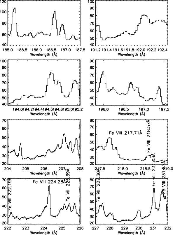
One of the original plates from B.C.Fawcett was found to contain very strong transition region lines, mostly from Fe VIII, Fe IX. The plate (C12h) was obtained from an Iron Carbonyl source using a grazing incidence spectrometer. The plate was scanned, and a portion of an averaged spectrum wavelength-calibrated. Spectral windows containing Fe VIII are shown in Fig. 8. Unfortunately, it is not possible to calibrate the intensities of the spectral lines, so the assessment is mainly done considering the wavelengths. However, observed line strengths are in rough agreement with the gf values. All the Fe VIII lines observed by EIS having large gf values are also present in the plate.
3.3 The Malinovsky & Heroux (1973) spectrum
Malinovsky & Heroux (1973) published an integrated-Sun spectrum covering the 50-300 Å range with a medium resolution (0.25 Å), taken with a grazing-incidence spectrometer flown on a rocket in 1969. For a long time this has been the best available spectrum in the 150-300 Å range. One of the main reason is the fact that the spectrum was photometrically calibrated with great accuracy. Indeed previous benchmark studies have shown agreement to within a few % between predicted and observed intensities.
4 Discussion
The Malinovsky & Heroux (1973)
rocket spectrum allows us to benchmark the atomic data for the
strongest EUV transitions.
The emissivity ratio curves are presented in Fig. 9,
both using the original and scaled collision strengths and a scaling constant
![]() .
The intensities were integrated over the full Sun when it was
relatively quiet, so it is expected that the plasma has a broad
multi-thermal distribution peaked around 1 MK; different
curves are not necessarily expected to cross. However, Fig. 9
clearly shows that the relative temperature sensitivity in the
lines is very small, so multi-thermal effects would also be small.
Overall, the comparison between observed and expected intensities
is satisfactory.
There is slightly better agreement (within
.
The intensities were integrated over the full Sun when it was
relatively quiet, so it is expected that the plasma has a broad
multi-thermal distribution peaked around 1 MK; different
curves are not necessarily expected to cross. However, Fig. 9
clearly shows that the relative temperature sensitivity in the
lines is very small, so multi-thermal effects would also be small.
Overall, the comparison between observed and expected intensities
is satisfactory.
There is slightly better agreement (within ![]() 20%) between
observed and expected intensities using the scaled collision strengths,
in particular when the 1-53 transition is considered.
This line has a mild temperature sensitivity and provides
log T[K] = 5.6.
However, this line is one of the three which had their intensity
obtained with a deconvolution method by Malinovsky & Heroux (1973),
so has a more uncertain strength.
20%) between
observed and expected intensities using the scaled collision strengths,
in particular when the 1-53 transition is considered.
This line has a mild temperature sensitivity and provides
log T[K] = 5.6.
However, this line is one of the three which had their intensity
obtained with a deconvolution method by Malinovsky & Heroux (1973),
so has a more uncertain strength.
|
Figure 9:
The emissivity ratio curves relative to the
Malinovsky & Heroux (1973) spectrum,
using the original G00 collision strengths (above) and the scaled ones (below).
|
| Open with DEXTER | |
|
Figure 10: The emissivity ratio curves relative to the ``foreground-subtracted'' Sunspot loop leg observed by EIS using the original G00 collision strengths (above) and the scaled ones (below), for the strongest transitions in the SW channel. |
| Open with DEXTER | |
Malinovsky & Heroux (1973) only observed the two brightest transitions at the EIS wavelengths, at 185.21, 186.60 Å, because of the lower spectral resolution and the averaging over the whole Sun of the rocket spectrum did not allow observations of the weaker lines. Notice that these strong 185.21 and 186.60 Å lines, in normal active region observations, would be partially blended with Ni XVI and Ca XIV.
The EIS spectra allow us to consider further weaker lines.
Figs. 10, 11, 13
show the emissivity ratio curves for the
``foreground-subtracted'' Sunspot loop leg, all
calculated at an electron density of 109 cm-3 and
the same scaling constant
![]() (so they are directly comparable).
The observed intensities
(so they are directly comparable).
The observed intensities
![]() are
in phot cm-2 s-1 arcsec-1.
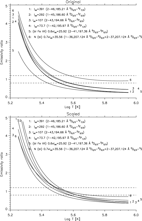
Figure 10 shows the curves for the six strongest
transitions observed in the SW channel.
The 2-43 194.66 Å and 1-42 195.97 Å are
strong transitions which appear unblended.
The 20% discrepancy (when using the original collision strengths)
between the 2-46, 1-45 and the
2-43, 1-42 transitions confirms the benchmark calculation results:
the first two transitions have too large gf values, hence
too large collision strengths, which in turns increases the
theoretical intensities, and lowers the emissivity ratio curves.
A slightly better agreement is found when the scaled
collision strengths are used.
Notice that about 40% of the intensity of the
2-41 197.36 Å line appears to be due to an Fe VII line
(Del Zanna 2009), so the observed intensity has been
corrected by this amount. Very good agreement is found with the
scaled collision strengths.
The 1-36 3p63d 2D3/2-3p53d2 2D5/2 and
2-37 3p63d 2D5/2-3p53d2 4S3/2 transitions are
expected to be close in wavelength and strong. They are identified here
as a self-blend observed at 207.124 Å, considering that no other nearby
lines (see Fig. 4) have the appropriate intensity
and morphology. About 30% of the observed intensity still
appears unaccounted for.
are
in phot cm-2 s-1 arcsec-1.
Figure 10 shows the curves for the six strongest
transitions observed in the SW channel.
The 2-43 194.66 Å and 1-42 195.97 Å are
strong transitions which appear unblended.
The 20% discrepancy (when using the original collision strengths)
between the 2-46, 1-45 and the
2-43, 1-42 transitions confirms the benchmark calculation results:
the first two transitions have too large gf values, hence
too large collision strengths, which in turns increases the
theoretical intensities, and lowers the emissivity ratio curves.
A slightly better agreement is found when the scaled
collision strengths are used.
Notice that about 40% of the intensity of the
2-41 197.36 Å line appears to be due to an Fe VII line
(Del Zanna 2009), so the observed intensity has been
corrected by this amount. Very good agreement is found with the
scaled collision strengths.
The 1-36 3p63d 2D3/2-3p53d2 2D5/2 and
2-37 3p63d 2D5/2-3p53d2 4S3/2 transitions are
expected to be close in wavelength and strong. They are identified here
as a self-blend observed at 207.124 Å, considering that no other nearby
lines (see Fig. 4) have the appropriate intensity
and morphology. About 30% of the observed intensity still
appears unaccounted for.
|
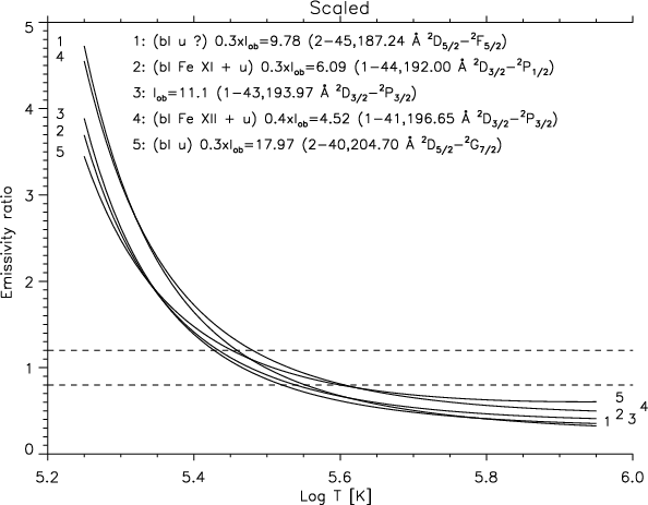
Figure 11: The emissivity ratio curves relative to the ``foreground-subtracted'' Sunspot loop leg observed by EIS for a few weaker transitions, using the scaled collision strengths. |
| Open with DEXTER | |
Figure 11 shows the emissivity ratio curves for a few weaker transitions. With the exception of the 1-43 193.97 Å transition, all lines appear to be blended. Notice that the 196.65 Å line in normal conditions would be blended with the strong Fe XII 196.64 Å transition, important for density diagnostics (Del Zanna & Mason 2005). A further 60% of the observed intensity must be due to an unidentified TR line. The weak 187.24 Å also appears to be significantly blended with another TR line.
The 1-44 3p63d 2D3/2-3p53d2 2P1/2 transition was only tentatively identified by RR80 with a line observed at 192.004. The EIS spectra do show a TR line at 192.000 Å which is most probably this transition, blended by 60% with another, stronger TR line. Other possibilities are a TR line observed at 192.087 Å, which however has a morphology closer to Fe IX, and the 191.585 Å line, which is most probably a Mn IX transition (see Table 4, the laboratory spectrum in Fig. 8, the EIS one in Fig. 4, and the morphology in Fig. 2). Notice that the 192.000 Å line is of particular importance because it blends, together with an Fe XI transition (Del Zanna et al. 2009), with the flare Fe XXIV line (Del Zanna 2006).
The 2-40 3p63d 2D5/2-3p53d2 2G7/2 line ought to be well observed in the EIS spectrum. The only TR lines close in wavelength and predicted intensity are those observed at 204.704 and 205.040 Å. The 205.040 and 205.708 Å lines have the correct wavelengths and intensity ratio to be identified with two strong Cr VIII transitions, firstly identified by G65 (the strongest Cr VII transition at 200.83 Å is also a prominent line in the spectrum, which confirms the presence of Cr lines). This leaves the 204.704 Å as the only possibility, although the predicted intensity is less than half of what is observed. Note that this line is important because it is blended with one of the two strongest Fe XVII lines observable by EIS (Del Zanna & Ishikawa 2009).
All the lines observed by EIS are also present in the laboratory spectrum of Fig. 8. In the 211-246 Å range, the spectrum contained 5 of the strong Fe VIII lines originally identified by RR80, plus 3 transitions identified here (see Table 4 for the measurements and Table 3 for the spectroscopic identification). These 8 transitions are labelled in Fig. 8.
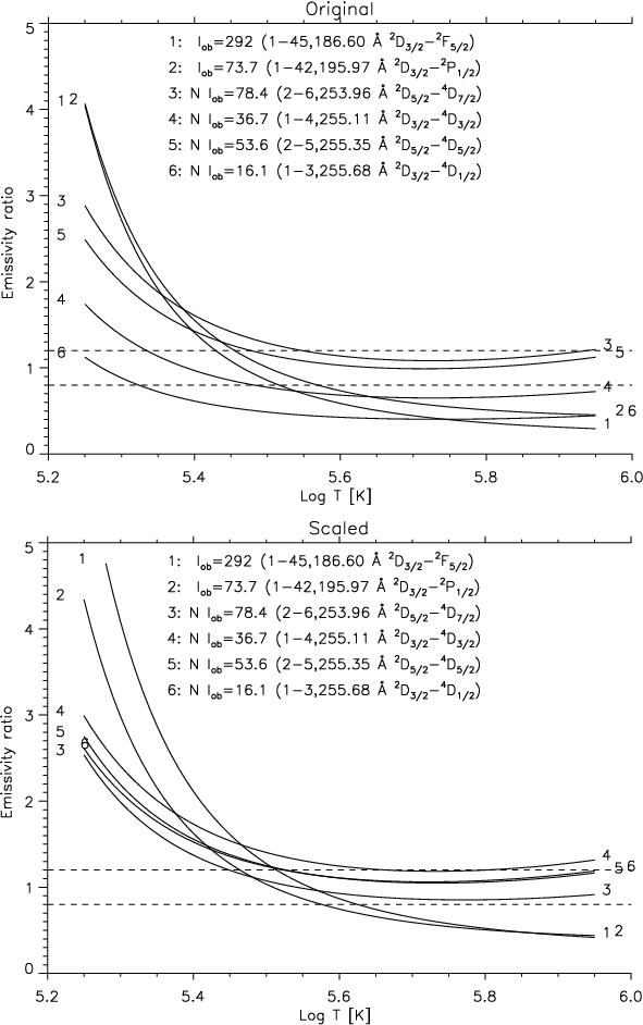
4.1 Identification of the 4Dj levels and the
possibility of measuring

The strong lines of the 3p6 3d 2Dj-3p5 3d2 4Dj transition array were not previously identified. They are predicted to be strong and fall within the EIS wavelength range. There are only few candidate lines, based on morphology arguments, but when the theoretical splittings of the 4Dj levels is considered, there are no options. The four strong lines around 255 Å seen in Fig. 4 are clearly lines from this array. The agreement between the measured and theoretical splittings of the 4Dj levels is excellent, as shown in Table 2.
These lines are particularly important because they provide a direct way to measure the electron temperature, when combined with lines decaying from higher levels. Before discussing the emissivity ratios for these lines, however, the temperature distribution of the plasma needs to be considered.
One well-established way to estimate the temperature distribution of the emitting plasma is the so-called emission measure loci method, whereby the observed intensities, divided by their contribution functions, are plotted as a function of the electron temperature. For a description of the method, see e.g. Del Zanna et al. (2002). When introduced for the first time to the study of active region loops observed with the SOHO/CDS spectrometer, this method has consistently indicated that the legs of active region loops seem to have a near-isothermal temperature distribution (Del Zanna & Mason 2003; Del Zanna 2003). This means that the various ions are emitting at temperatures which can be well below or well above the temperature of peak ion abundance in equilibrium.
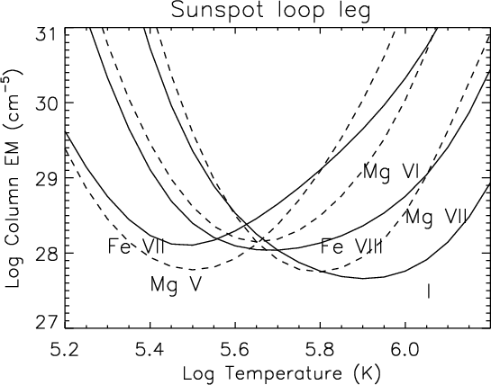
A similar situation applies to the Sunspot loop leg examined here. Figure 12 shows the EM Loci plots for three Mg lines (Mg V 276.58 Å, Mg VI 270.39 Å, Mg VII 278.4 Å deblended from Si VII) and three Fe lines: Fe VII 176.74 Å, Fe VIII 186.61 Å, and Fe IX 171.07 Å. The atomic data used for Fe VII are described in Del Zanna (2009), while for Fe VIII the scaled collision strengths are used. For Fe IX and the Mg ions, CHIANTI v.5.2 (Landi et al. 2006) was used.
The new CHIANTI v.6 (Dere et al. 2009) ion abundances (in ionization equilibrium) were used for the EM Loci plot. The EM Loci of the Mg lines in Fig. 12 are consistent with an isothermal plasma having log T [K] = 5.65. Curves from other ions, not shown here, also cluster around log T [K] = 5.6, as are those from the Fe ions. If ionization equilibrium holds, and the ion abundances are correct, one would then expect to measure similar values from intensity ratios of lines sensitive to temperature. Moreover, the emissivity ratio curves should all cross at log T [K] = 5.65.
A few caveats however apply. First, some departures from ionization equilibrium caused by the strong down-flows (of the order of 30-50 km s-1 along the structure) are to be expected. For the upper-transition-region ions such as Fe VIII, Fe IX, the down-flows would naturally lower the electron temperature at which lines are formed (Raymond & Dupree 1978). The fact that the plasma is mainly radiatively cooling (Bradshaw 2008), would also lower the measured electron temperature compared to equilibrium values. This issue will be addressed in a follow-up paper. Second, large uncertainties are associated with ionization equilibrium curves, for a variety of reasons (see e.g. some issues discussed in Del Zanna et al. 2002). Also notice that the new CHIANTI v.6 equilibrium curves are significantly different from previous ones, in particular for the Fe ions, where the peak ion abundance is now shifted toward much lower temperatures. The excellent agreement in the morphology of Si VII, Mg VII, and Fe VIII lines (see, e.g. Fig. 2, 3) suggests a possible discrepancy in the temperature calculated in collisional equilibrium for Fe VIII (log T [K] = 5.6), compared to Si VII and Mg VII (log T [K] = 5.8). Third, even if a loop cross-section is nearly isothermal, line-of-sight effects can always affect the measurements.
|
Figure 12: Emission measure loci plot relative to the ``foreground-subtracted'' Sunspot loop leg observed by EIS. |
| Open with DEXTER | |
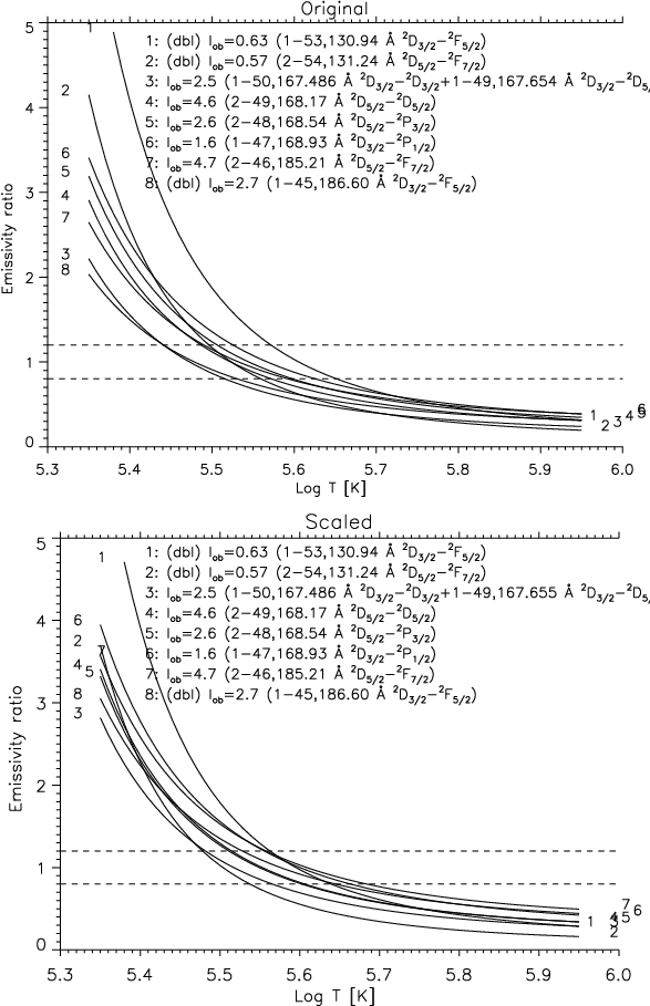
The emissivity ratio curves for the lines of the 3p6 3d 2Dj-3p5 3d2 4Dj transition array are shown in Fig. 13, both using the original G00 collision strengths and the scaled ones. The curves relative to the two strong decays 1-45 186.60 Å and 1-42 195.97 Å are also displayed. There are large disagreements between the observed and expected intensities when the original data are used. Also, the strongest transitions would indicate a log T [K] = 5.4, far below the temperature from the EM Loci method. The scaled data provide a much better agreement between observed and expected intensities, and higher temperatures (about log T [K] = 5.5), although the scatter in the curves is still quite large.
|
Figure 13: The emissivity ratio curves relative to the ``foreground-subtracted'' Sunspot loop leg observed by EIS using the original G00 collision strengths and the scaled ones. |
| Open with DEXTER | |
5 Summary and conclusions
From the various atomic structure calculations published and
presented here, it is clear that the excitation rates of G00
need to be improved.
A large scattering calculation for this ion is non-trivial, so for this benchmark
work the G00 rates of the dipole-allowed
transitions have been scaled using a large benchmark calculation.
Large uncertainties in the predicted line intensities
are obviously still present, however the comparison
with the Hinode/EIS and the Malinovsky & Heroux (1973)
intensities is very satisfactory, with agreement within ![]() 20%
for all the strongest transitions, when the scaled
collision strengths are considered.
The excellent agreement between the Hinode/EIS
wavelengths and the RR80 ones is very satisfactory, and shows
that with a detailed analysis, very accurate wavelengths
can be obtained with the EIS spectra.
20%
for all the strongest transitions, when the scaled
collision strengths are considered.
The excellent agreement between the Hinode/EIS
wavelengths and the RR80 ones is very satisfactory, and shows
that with a detailed analysis, very accurate wavelengths
can be obtained with the EIS spectra.
The predicted line intensities, combined with a detailed analysis of Hinode/EIS and laboratory spectra, allowed the identification of several new transitions, and confirm the previous ones from G65 and RR80. However, a few lines which should be observable in astrophysical spectra are still not identified, and in a large number of cases Fe VIII lines in the EIS spectra appear to be blended.
Of particular importance are the newly identified strong lines of the 3p6 3d 2Dj-3p5 3d2 4Dj transition array because it is shown here that they can provide a direct measurement of the electron temperature. Previous Skylab observations produced contradictory results in terms of loop electron temperatures from line ratios in the upper transition region. For example, Raymond & Foukal (1982) found a very low electron temperature from the resonance vs. intercombination Ne VII ratio (log T [K] = 5.3 instead of the equilibrium 5.75) in loops observed at the limb. Doyle et al. (1985) used the same Ne VII ratio on a Sunspot loop but found an equilibrium temperature (consistent departures were found in lower-temperature ions).
The EIS observations indicate that loop legs have lower temperatures than predicted in ionization equilibrium for Fe VIII. This is not surprising; however, firm measurements will only be possible once better scattering calculations are available, and the EIS radiometric calibration is properly assessed. Evidencewas found in a number of cases (Del Zanna & Ishikawa 2009; Del Zanna 2008a) for lines around 250 Å having significantly lower intensities than expected.
It is obviously important to attempt measurements of electron temperatures which are independent of any assumption of ionization equilibrium. Further observational constraints and non-equilibrium forward-modeling such as that of Bradshaw et al. (2004) will shed some light on this issue.
AcknowledgementsSupport from STFC (Advanced Fellowship and APAP network) is acknowledged. I warmly thank B.C. Fawcett for helping in identify some of the best plates of his archive, and staff at RAL (P.R.Young and J.Payne) for their help. I also thank N.R. Badnell, H.E. Mason and especially two anonymous referees for their useful comments which helped to improve the manuscript. The analysis of the Hinode/EIS observation presented here was stimulated by the participation to the Coronal Loop Workshop held in Santorini in June 2007, where some results concerning the EIS/TRACE cross-calibration were presented. Hinode is a Japanese mission developed and launched by ISAS/JAXA, with NAOJ as domestic partner and NASA and STFC (UK) as international partners. It is operated by these agencies in co-operation with ESA and NSC (Norway).
References
- Badnell, N. R. 1997, J. Phys. B Atom. Mol. Phys., 30, 1 [NASA ADS] [CrossRef]
- Behring, W. E., Cohen, L., Doschek, G. A., & Feldman, U. 1976, ApJ, 203, 521 [NASA ADS] [CrossRef]
- Bradshaw, S. J. 2008, A&A, 486, L5 [NASA ADS] [CrossRef] [EDP Sciences]
- Bradshaw, S. J., Del Zanna, G., & Mason, H. E. 2004, A&A, 425, 287 [NASA ADS] [CrossRef] [EDP Sciences]
- Brown, C. M., Feldman, U., Seely, J. F., Korendyke, C. M., & Hara, H. 2008, ApJS, 176, 511 [NASA ADS] [CrossRef]
- Burgess, A., & Tully, J. A. 1992, A&A, 254, 436 [NASA ADS]
- Culhane, J. L., Harra, L. K., James, A. M., et al. 2007, Sol. Phys., 60
- Del Zanna, G. 2003, A&A, 406, L5 [NASA ADS] [CrossRef] [EDP Sciences]
- Del Zanna, G. 2006, A&A, 447, 761 [NASA ADS] [CrossRef] [EDP Sciences]
- Del Zanna, G. 2007, in ASPC, Vol. 397, First Science results from Hinode, 87
- Del Zanna, G. 2008a, A&A, 481, L69 [NASA ADS] [CrossRef] [EDP Sciences]
- Del Zanna, G. 2008b, A&A, 481, L49 [NASA ADS] [CrossRef] [EDP Sciences]
- Del Zanna, G. 2009, A&A, 508, 501 [CrossRef] [EDP Sciences]
- Del Zanna, G., & Ishikawa, Y. 2009, A&A, accepted
- Del Zanna, G., & Mason, H. E. 2003, A&A, 406, 1089 [NASA ADS] [CrossRef] [EDP Sciences]
- Del Zanna, G., & Mason, H. E. 2005, A&A, 433, 731 [NASA ADS] [CrossRef] [EDP Sciences]
- Del Zanna, G., Landini, M., & Mason, H. E. 2002, A&A, 385, 968 [NASA ADS] [CrossRef] [EDP Sciences]
- Del Zanna, G., Berrington, K. A., & Mason, H. E. 2004, A&A, 422, 731 [NASA ADS] [CrossRef] [EDP Sciences]
- Del Zanna, G., Storey, P. J., & Mason, H. E. 2009, A&A, in press
- Dere, K. P., Landi, E., Mason, H. E., Monsignori Fossi, B. C., & Young, P. R. 1997, A&AS, 125, 149 [NASA ADS] [CrossRef] [EDP Sciences]
- Dere, K. P., Landi, E., Young, P. R., et al. 2009, A&A, 498, 915 [NASA ADS] [CrossRef] [EDP Sciences]
- Doyle, J. G., Raymond, J. C., Noyes, R. W., & Kingston, A. E. 1985, ApJ, 297, 816 [NASA ADS] [CrossRef]
- Flower, D. R., & Nussbaumer, H. 1974, A&A, 31, 353 [NASA ADS]
- Gabriel, A. H., Fawcett, B. C., & Jordan, C. 1965, Nature, 206, 390 [NASA ADS] [CrossRef]
- Griffin, D. C., Pindzola, M. S., & Badnell, N. R. 2000, A&AS, 142, 317 [NASA ADS] [CrossRef] [EDP Sciences]
- Haugan, S. V. H. 1997, CDS software note, 47
- Ishikawa, Y., & Vilkas, M. J. 2008, Phys. Rev. A, 78, 042501 [NASA ADS] [CrossRef]
- Kruger, P. G., & Weissberg, S. G. 1937, Phys. Rev., 52, 314 [NASA ADS] [CrossRef]
- Landi, E., Del Zanna, G., Young, P. R., et al. 2006, ApJS, 162, 261 [NASA ADS] [CrossRef]
- Malinovsky, L., & Heroux, M. 1973, ApJ, 181, 1009 [NASA ADS] [CrossRef]
- Nussbaumer, H., & Storey, P. J. 1978, A&A, 64, 139 [NASA ADS]
- Ramonas, A. A., & Ryabtsev, A. N. 1980, Optics and Spectroscopy, 48, 348 [NASA ADS]
- Raymond, J. C., & Dupree, A. K. 1978, ApJ, 222, 379 [NASA ADS] [CrossRef]
- Raymond, J. C., & Foukal, P. 1982, ApJ, 253, 323 [NASA ADS] [CrossRef]
- Young, P. R., Del Zanna, G., Mason, H. E., et al. 2007, PASJ, 59, 727 [NASA ADS]
- Zeippen, C. J., Seaton, M. J., & Morton, D. C. 1977, MNRAS, 181, 527 [NASA ADS]
- Zeng, J., Jin, F., Zhao, G., & Yuan, J. 2003, J. Phys. B Atom. Mol. Phys., 36, 3457 [NASA ADS] [CrossRef]
Footnotes
- ...
CHIANTI
![[*]](/icons/foot_motif.png)
- http://www.chianti.rl.ac.uk
- ... database
- http://physics.nist.gov/PhysRefData/ASD/index.html
All Tables
Table 1: Electron configuration basis for the benchmark calculation (23C) and orbital scaling parameters.
Table 2: Level energies for Fe VIII.
Table 3: List of strongest Fe VIII lines in the 100-500 Å range.
Table 4: List of measured wavelengths.
All Figures
|
|
Figure 1: Top: thermally-averaged collisions strengths for the 2-46 transition. The dashed line indicates the original calculated values from G00, while the continuous one the scaled values (see text). Bottom: the same points, plotted in the scaled domain (Burgess & Tully 1992), with the high-temperature limits (scaled temperature = 1). |
| Open with DEXTER | |
| In the text | |
|
|
Figure 2: Monochromatic images (negative) of the Fe VIII identified lines observed by EIS. Notice that all the Fe VIII lines have a similar morphology. |
| Open with DEXTER | |
| In the text | |
|
|
Figure 3: Monochromatic images (negative) of a selection of EIS lines (ion and wavelength in Å are indicated together with the logarithm of the temperature (K) of formation of the lines in collisional ionization equilibrium). Notice the large morphological differences in lines formed at different temperatures. |
| Open with DEXTER | |
| In the text | |
|
|
Figure 4: Hinode EIS spectra (units are average counts per pixel) over three different areas. Thick lines refer to the spectrum over the Sunspot leg, where Fe VIII lines were clearly strong. The thick grey line shows the foreground Sunspot spectrum, while the thin black spectrum is from the reference area used for the wavelength calibration. |
| Open with DEXTER | |
| In the text | |
|
|
Figure 5:
Enlarged portion of the Fe VIII 186.60 Å radiance
(negative image, SW channel),
with contours of the Si VII 275.35 Å intensity (LW channel), showing
agreement to within 1
|
| Open with DEXTER | |
| In the text | |
|
|
Figure 6: Top: Doppler-gram of the Si VII 275.35 Å line showing strong (20 km s-1 or more) red-shifts in the legs of the coronal loops. The location of the area chosen to obtain averaged spectra from a Sunspot loop leg is indicated by the crossing of the two sets of dashed lines. Bottom: a slice along the N-S dashed lines of the Doppler-shifts in two lines in the SW and LW channels. Despite the lack of simultaneity between the channels, good agreement is found. The dashed lines indicate the location of the chosen Sunspot loop leg area (having a red-shift of about 20 km s-1). |
| Open with DEXTER | |
| In the text | |
|
|
Figure 7: Difference between fitted and theoretical wavelengths (Å) in the SW and LW channels of EIS. A linear dispersion for the SW channel was used, while a quadratic one was adopted for the LW. |
| Open with DEXTER | |
| In the text | |
|
|
Figure 8: Spectral windows from the laboratory plate (arbitrary units) containing Fe VIII lines. The first five wavelength ranges are the same as those reported in Fig. 4, while the last ones show regions not observed by Hinode EIS. |
| Open with DEXTER | |
| In the text | |
|
|
Figure 9:
The emissivity ratio curves relative to the
Malinovsky & Heroux (1973) spectrum,
using the original G00 collision strengths (above) and the scaled ones (below).
|
| Open with DEXTER | |
| In the text | |
|
|
Figure 10: The emissivity ratio curves relative to the ``foreground-subtracted'' Sunspot loop leg observed by EIS using the original G00 collision strengths (above) and the scaled ones (below), for the strongest transitions in the SW channel. |
| Open with DEXTER | |
| In the text | |
|
|
Figure 11: The emissivity ratio curves relative to the ``foreground-subtracted'' Sunspot loop leg observed by EIS for a few weaker transitions, using the scaled collision strengths. |
| Open with DEXTER | |
| In the text | |
|
|
Figure 12: Emission measure loci plot relative to the ``foreground-subtracted'' Sunspot loop leg observed by EIS. |
| Open with DEXTER | |
| In the text | |
|
|
Figure 13: The emissivity ratio curves relative to the ``foreground-subtracted'' Sunspot loop leg observed by EIS using the original G00 collision strengths and the scaled ones. |
| Open with DEXTER | |
| In the text | |
Copyright ESO 2009
Current usage metrics show cumulative count of Article Views (full-text article views including HTML views, PDF and ePub downloads, according to the available data) and Abstracts Views on Vision4Press platform.
Data correspond to usage on the plateform after 2015. The current usage metrics is available 48-96 hours after online publication and is updated daily on week days.
Initial download of the metrics may take a while.