| Issue |
A&A
Volume 508, Number 1, December II 2009
|
|
|---|---|---|
| Page(s) | 259 - 274 | |
| Section | Interstellar and circumstellar matter | |
| DOI | https://doi.org/10.1051/0004-6361/200811099 | |
| Published online | 15 October 2009 | |
A&A 508, 259-274 (2009)
Dense and warm molecular gas in the envelopes and outflows of southern low-mass protostars
T. A. van Kempen1,2 - E. F. van Dishoeck1,3 - M. R. Hogerheijde1 - R. Güsten4
1 - Leiden Observatory, Leiden University, PO Box 9513, 2300 RA Leiden, The Netherlands
2 - Center for Astrophysics, 60 Garden Street, MS 78, Cambridge, MA 02138, USA
3 - Max Planck Institut für Extraterrestrische Physik (MPE), Giessenbachstr. 1, 85748 Garching, Germany
4 - Max Planck Institut für Radioastronomie, Auf dem Hügel 69, 53121 Bonn, Germany
Received 7 October 2008 / Accepted 6 October 2009
Abstract
Context. Observations of dense molecular gas lie at the
basis of our understanding of the density and temperature structure of
protostellar envelopes and molecular outflows. The Atacama Pathfinder
EXperiment (APEX) opens up the study of southern (Dec
![]() )
protostars.
)
protostars.
Aims. We aim to characterize the properties of the protostellar
envelope, molecular outflow and surrounding cloud, through observations
of high excitation molecular lines within a sample of 16 southern
sources presumed to be embedded YSOs, including the most luminous
Class I objects in Corona Australis and Chamaeleon.
Methods. Observations of submillimeter lines of CO, HCO+ and their isotopologues, both single spectra and small maps (up to
![]() ),
were taken with the FLASH and APEX-2a instruments mounted on APEX to
trace the gas around the sources. The HARP-B instrument on the JCMT was
used to map IRAS 15398-3359 in these lines. HCO+ mapping
probes the presence of dense centrally condensed gas, a characteristic
of protostellar envelopes. The rare isotopologues C18O and H13CO+
are also included to determine the optical depth, column density, and
source velocity. The combination of multiple CO transitions, such as
3-2, 4-3 and 7-6, allows to constrain outflow properties, in particular
the temperature. Archival submillimeter continuum data are used to
determine envelope masses.
),
were taken with the FLASH and APEX-2a instruments mounted on APEX to
trace the gas around the sources. The HARP-B instrument on the JCMT was
used to map IRAS 15398-3359 in these lines. HCO+ mapping
probes the presence of dense centrally condensed gas, a characteristic
of protostellar envelopes. The rare isotopologues C18O and H13CO+
are also included to determine the optical depth, column density, and
source velocity. The combination of multiple CO transitions, such as
3-2, 4-3 and 7-6, allows to constrain outflow properties, in particular
the temperature. Archival submillimeter continuum data are used to
determine envelope masses.
Results. Eleven of the sixteen sources have associated warm and/or dense (![]() 106 cm-3)
quiescent gas characteristic of protostellar envelopes, or an
associated outflow. Using the strength and degree of concentration of
the HCO+ 4-3 and CO 4-3 lines as a diagnostic, five sources
classified as Class I based on their spectral energy distributions
are found not to be embedded YSOs. The C18O 3-2 lines show
that for none of the sources, foreground cloud layers are present.
Strong molecular outflows are found around six sources, with outflow
forces an order of magnitude higher than for previously studied
Class I sources of similar luminosity.
106 cm-3)
quiescent gas characteristic of protostellar envelopes, or an
associated outflow. Using the strength and degree of concentration of
the HCO+ 4-3 and CO 4-3 lines as a diagnostic, five sources
classified as Class I based on their spectral energy distributions
are found not to be embedded YSOs. The C18O 3-2 lines show
that for none of the sources, foreground cloud layers are present.
Strong molecular outflows are found around six sources, with outflow
forces an order of magnitude higher than for previously studied
Class I sources of similar luminosity.
Conclusions. This study provides a starting point for future
ALMA and Herschel surveys by identifying truly embedded southern YSOs
and determining their larger scale envelope and outflow
characteristics.
Key words: astrochemistry - stars: formation - submillimeter - ISM: jets and outflows - ISM: molecules
1 Introduction
During the early stages of low-mass star formation, young stellar objects (YSOs) are embedded in cold dark envelopes of gas and dust, which absorb the radiation from the central star (Lada 1987; André et al. 1993). This extinction is strong enough that low-mass embedded YSOs, or protostars, only emit weakly at infrared wavelengths (e.g., Jørgensen et al. 2005b; Gutermuth et al. 2008). Only at later evolutionary phases, in which the envelope has been accreted and/or dispersed, does emission in the optical and infrared (IR) dominate the spectral energy distribution (SED) (e.g. Hartmann et al. 2005). Protostars emit the bulk of their radiation at far-IR and sub-millimeter wavelengths, both as continuum radiation, produced by the cold (T < 30 K) dust, and through molecular line emission from the gas-phase species present throughout the protostellar envelope. Although the bulk of the mass is accreted during the earliest embedded phases, more evolved protostellar envelopes still contain a reservoir of gas and dust that can accrete onto the central star and disk system and thus provide the material for disk and planet formation. At the same time, jets and winds from the young star interact with the envelope and drive molecular outflows which clear the surroundings. Characterizing and quantifying all of these different physical components in the protostellar stage is still a major observational challenge.
The protostellar envelopes and molecular outflows can be directly observed either through thermal emission of dust at (sub)millimeter wavelengths (e.g. Shirley et al. 2000; Johnstone et al. 2001; Nutter et al. 2005) or the line emission of molecules. Low frequency molecular emission traces the cold gas in the protostellar envelopes (e.g., Hogerheijde et al. 1998; Jørgensen et al. 2002; Maret et al. 2004) or molecular outflows (e.g., Snell et al. 1990; Cabrit & Bertout 1992; Bachiller & Tafalla 1999). Single-dish observations of dust using current generation bolometer arrays are able to map large areas and image the surroundings of protostars (e.g., Motte et al. 1998; Shirley et al. 2000; Stanke et al. 2006; Nutter et al. 2008). Through radiative transfer models (e.g., Shirley et al. 2002; Jørgensen et al. 2002; Young et al. 2003), including information from shorter wavelengths (e.g., Hatchell et al. 2007b), the temperature and density structure of the protostellar envelope can be constrained, but the continuum data cannot determine the velocity structure of the infalling envelope, characterize the outflows and their interaction with the surroundings, or disentangle envelope and (foreground) cloud material. Analysis of gas observations in the form of spectra of multiple transitions of the same molecule and its isotopologues provide additional strong constraints on the physical characteristics of the protostellar envelope (Mangum & Wootten 1993; Blake et al. 1994; van Dishoeck et al. 1995; Schöier et al. 2002; Maret et al. 2004; Jørgensen et al. 2005b; Evans et al. 2005; van der Tak et al. 2007) and outflowing gas (e.g., Cabrit & Bertout 1992; Bontemps et al. 1996; Hogerheijde et al. 1998; Hatchell et al. 1999; Parise et al. 2006; Hatchell et al. 2007a).
Although many different molecules have been observed in protostellar
envelopes, only a limited number of species are well suited to trace
the physical characteristics of all of the components of an embedded
YSO and its surroundings. For example, the use of CH3OH and
H2CO is complicated by their changing abundances through the
envelope, although some information can be obtained with careful
analysis and a sufficient number of observed lines
(e.g. Mangum & Wootten 1993; Blake et al. 1994; van Dishoeck et al. 1995;
van der Tak et al. 2000; Leurini et al. 2004). The weakness of high-excitation CH3OH and H2CO lines in all but a handful of the most luminous Class 0 protostars
(e.g. Jørgensen et al. 2005a) coupled with a lack of some
collisional rate coefficients make these species less suitable tracers for
the bulk of the low-mass embedded YSOs.
In practice, the column density of the surrounding cloud (and that of
any unrelated foreground clouds) is best probed by low excitation
optically thin transitions of molecules with a low dipole moment, such
as the isotopologues of CO, e.g., C18O 2-1 or 3-2
(van Kempen et al. 2009b). For molecular outflows the line wings of various
12CO transitions have been efficiently used as tracers of their
properties
(Cabrit & Bertout 1992; Bontemps et al. 1996; Hogerheijde et al. 1998; Bachiller & Tafalla 1999; Hatchell et al. 1999; Hatchell et al. 2007a).
The denser regions of the protostellar envelope need to be probed with
emission lines with a high critical density, such as the higher
excitation transitions from HCO+ with critical densities >106 cm-3. The warm gas (T
> 50 K), which can be present in both the molecular outflow and
the inner region of the protostellar envelope, can only be traced by
spectrally resolved high-J CO transitions,
which have
![]() K for
K for
![]() (Hogerheijde et al. 1998).
(Hogerheijde et al. 1998).
Embedded YSOs are generally identified by their 2-24 ![]() m IR slope
with positive values characteristic of Class I objects (Lada 1987).
Over the last several years, it has been found that some of these
Class I objects turn out to be edge-on disks or obscured sources
(e.g., Luhman & Rieke 1999; Brandner et al. 2000; Pontoppidan et al. 2005; Lahuis et al. 2006; van Kempen et al. 2009b).
The use of a spectral line map over a small (
m IR slope
with positive values characteristic of Class I objects (Lada 1987).
Over the last several years, it has been found that some of these
Class I objects turn out to be edge-on disks or obscured sources
(e.g., Luhman & Rieke 1999; Brandner et al. 2000; Pontoppidan et al. 2005; Lahuis et al. 2006; van Kempen et al. 2009b).
The use of a spectral line map over a small (![]()
![]() )
region around the protostar is an elegant solution to disentangle the
contributions of the different components (Boogert et al. 2002). In
particular, the spatial distribution of the HCO+ 4-3 line has
proven to be an excellent diagnostic of such ``false'' embedded sources:
in the case of Ophiuchus, about 60% of the sources with Class I or
flat SED slopes turned out not to be embedded YSOs
(van Kempen et al. 2009b).
)
region around the protostar is an elegant solution to disentangle the
contributions of the different components (Boogert et al. 2002). In
particular, the spatial distribution of the HCO+ 4-3 line has
proven to be an excellent diagnostic of such ``false'' embedded sources:
in the case of Ophiuchus, about 60% of the sources with Class I or
flat SED slopes turned out not to be embedded YSOs
(van Kempen et al. 2009b).
With the development of the Atacama large millimeter/submillimeter
array (ALMA) on Chajnantor, Chile, surveys of sources in southern
star-forming clouds will be undertaken at high resolution (![]() 1'') at a wide range of frequencies, and are expected to reveal much
about the inner structure of protostars and their circumstellar
disks. The Herschel space observatory will also target a large
number of low-mass YSOs across the sky. Both sets of observations
rely heavily on complementary large aperture ground-based single-dish
observations for planning and interpretation. Apart from providing
the necessary information about the structure on larger scales,
single-dish studies of low-mass star formation in the southern sky
will also put the results obtained from studies on the northern
hemisphere in perspective.
1'') at a wide range of frequencies, and are expected to reveal much
about the inner structure of protostars and their circumstellar
disks. The Herschel space observatory will also target a large
number of low-mass YSOs across the sky. Both sets of observations
rely heavily on complementary large aperture ground-based single-dish
observations for planning and interpretation. Apart from providing
the necessary information about the structure on larger scales,
single-dish studies of low-mass star formation in the southern sky
will also put the results obtained from studies on the northern
hemisphere in perspective.
Due to a lack of sub-millimeter telescopes at high dry sites in the
southern hemisphere, high frequency data on southern YSOs are still
limited. The Swedish ESO submillimeter telescope (SEST) operated up to
the 345 GHz window, but for only limited periods of the year. As a
result, southern clouds, such as Chamaeleon, Corona Autralis, Vela or
Lupus, are much less studied than their counterparts in the northern
sky, such as Taurus and Perseus, where such observations have been
readily available for over a decade
(e.g., Hogerheijde et al. 1997; Motte et al. 1998; Hogerheijde et al. 1998; Johnstone et al. 2000; Jørgensen et al. 2002; Nutter et al. 2005; Nutter et al. 2008).
The Atacama Pathfinder EXperiment (APEX) (Güsten et al. 2006)![]() has opened up
access to the atmospheric windows in the 200-1400
has opened up
access to the atmospheric windows in the 200-1400 ![]() m wavelength
regime over the entire southern sky.
m wavelength
regime over the entire southern sky.
Of the southern star-forming regions not or only poorly visible with
northern telescopes two regions have proven especially interesting.
The Chamaeleon I cloud (D = 130 pc, Dec = ![]() ), observed with
IRAS and the Infrared Space Observatory (ISO) and included
in the Spitzer space telescope guaranteed time and ``Cores to
disks'' (c2d) Legacy programs (Persi et al. 2000; Evans et al. 2003; Damjanov et al. 2007; Luhman et al. 2008) contains some embedded
sources, especially around the Cederblad region
(Persi et al. 2000; Lehtinen et al. 2001; Belloche et al. 2006; Hiramatsu et al. 2007). Corona Australis
is a nearby star-forming region (D = 170 pc, see Knude & Høg (1998); Dec =
), observed with
IRAS and the Infrared Space Observatory (ISO) and included
in the Spitzer space telescope guaranteed time and ``Cores to
disks'' (c2d) Legacy programs (Persi et al. 2000; Evans et al. 2003; Damjanov et al. 2007; Luhman et al. 2008) contains some embedded
sources, especially around the Cederblad region
(Persi et al. 2000; Lehtinen et al. 2001; Belloche et al. 2006; Hiramatsu et al. 2007). Corona Australis
is a nearby star-forming region (D = 170 pc, see Knude & Høg (1998); Dec = ![]() ), well-known for the central Coronet cluster near the R
CrA star (Loren 1979; Taylor & Storey 1984; Wilking et al. 1986; Brown 1987). Large-scale
C18O 1-0 maps show that it contains about 50
), well-known for the central Coronet cluster near the R
CrA star (Loren 1979; Taylor & Storey 1984; Wilking et al. 1986; Brown 1987). Large-scale
C18O 1-0 maps show that it contains about 50 ![]() of gas
and dust (Harju et al. 1993). Many surveys have been undertaken in the IR
(e.g., Wilking et al. 1986; Wilking et al. 1997; Olofsson et al. 1999; Nisini et al. 2005), but only a
few studies mapped this region at submillimeter wavelengths
(Chini et al. 2003; Nutter et al. 2005). Although Corona Australis has only a few
protostars with rising infrared SEDs, the cloud does contains some of
the most luminous low-mass protostars in the neighborhood of the Sun
(D < 200 pc) with luminosities of up to 20
of gas
and dust (Harju et al. 1993). Many surveys have been undertaken in the IR
(e.g., Wilking et al. 1986; Wilking et al. 1997; Olofsson et al. 1999; Nisini et al. 2005), but only a
few studies mapped this region at submillimeter wavelengths
(Chini et al. 2003; Nutter et al. 2005). Although Corona Australis has only a few
protostars with rising infrared SEDs, the cloud does contains some of
the most luminous low-mass protostars in the neighborhood of the Sun
(D < 200 pc) with luminosities of up to 20
![]() .
.
In this paper we present observations of submillimeter lines of CO and HCO+ of a sample of 16 embedded sources in the southern sky, with a focus on the Chamaeleon I and Corona Australis clouds, to identify basic parameters such as column density, presence and influence of outflowing material, presence of warm and dense gas and the influence of the immediate surroundings, in preparation for Herschel and ALMA surveys or in-depth high resolution interferometric observations. In Sect. 2 we present the observations, for which the results are given in Sect. 3 with a distinction between the clouds and isolated sources. Both the single spectra (Sect. 3.1) and maps (Sect. 3.2) are presented. In Sect. 4 we perform the analysis of the observations, making use of archival submillimeter continuum data, with the final conclusions given in Sect. 5.
Table 1: Source sample.
2 Technical information
2.1 Source list
Sources were selected from a sample of sources with rising infrared
SEDs (Class I) observed with the InfraRed Spectrograph (IRS) on Spitzer in the scope of the c2d legacy program (Evans et al. 2003) and
with the very large telescope (VLT) of the European Southern
Observatory (Pontoppidan et al. 2003) (Table 1). At the time of selection of the Spitzer and VLT sources in 2000, the list included the
bulk of the known southern low-mass Class I YSOs with mid-infrared
fluxes of at least 100 mJy. Most of these sources are located in the
Chamaeleon and Corona Australis clouds, supplemented by a few other
isolated Class I sources found initially by IRAS.
Within the Chamaeleon I cloud,
most sources are located in the Cederblad region (Persi et al. 2000; Hiramatsu et al. 2007). Cha IRS 6a is located 6'' away from Ced
110 IRS 6 (![]() half an APEX beam at 460 GHz). Ced 110 IRS 4 was studied by Belloche et al. (2006) which detect an outflow with an axis of <30
half an APEX beam at 460 GHz). Ced 110 IRS 4 was studied by Belloche et al. (2006) which detect an outflow with an axis of <30![]() ,
which makes this source a prime target in Chamaeleon.
The embedded YSOs in the Corona Australis region are mostly located in the small region around R CrA, called the Coronet (Wilking et al. 1986; Wilking et al. 1997; Nutter et al. 2005),
but two sources are located in the R CrA B region. RCrA
IRS 7A and B are believed to be two embedded objects in a
wide binary configuration with a separation of 30'' (Nutter et al. 2005; Schöier et al. 2006). These are deeply embedded as little to no IR counterparts were found (Groppi et al. 2007). HH 100 is in a region that is dominated by the RCrA A complex, but is an embedded source in itself according to Nutter et al. (2005).
CrA IRAS 32 is located in R CrA B region, but has little
to none known surrounding material. HH 46 is a Class I
protostar famous for its well-characterized outflow, pointed to the
south-west
(Chernin & Masson 1991; Heathcote et al. 1996; Stanke et al. 1999; Noriega-Crespo et al. 2004; Velusamy et al. 2007). It is extensively discussed in van Kempen et al. (2009a). IRAS 12496-7650, also known as DK Cha, is one of the brightest protostars in the southern
hemisphere and a potential driving source of HH 54
(van Kempen et al. 2006). ISO-LWS observations were detected with ISO (Giannini et al. 1999), but not confirmed by van Kempen et al. (2006).
IRAS 07178-4429, IRAS 13546-3941 and IRAS 15398-3359, all
very interesting embedded sources in the southern hemisphere, are also
included
(e.g., Bourke et al. 1995; Shirley et al. 2000; Haikala et al. 2006). Table 1 lists the sources of our sample and their properties. Luminosities are adopted from the c2d lists (Evans et al. 2003, 2009) and the VLT lists (Pontoppidan et al. 2003).
,
which makes this source a prime target in Chamaeleon.
The embedded YSOs in the Corona Australis region are mostly located in the small region around R CrA, called the Coronet (Wilking et al. 1986; Wilking et al. 1997; Nutter et al. 2005),
but two sources are located in the R CrA B region. RCrA
IRS 7A and B are believed to be two embedded objects in a
wide binary configuration with a separation of 30'' (Nutter et al. 2005; Schöier et al. 2006). These are deeply embedded as little to no IR counterparts were found (Groppi et al. 2007). HH 100 is in a region that is dominated by the RCrA A complex, but is an embedded source in itself according to Nutter et al. (2005).
CrA IRAS 32 is located in R CrA B region, but has little
to none known surrounding material. HH 46 is a Class I
protostar famous for its well-characterized outflow, pointed to the
south-west
(Chernin & Masson 1991; Heathcote et al. 1996; Stanke et al. 1999; Noriega-Crespo et al. 2004; Velusamy et al. 2007). It is extensively discussed in van Kempen et al. (2009a). IRAS 12496-7650, also known as DK Cha, is one of the brightest protostars in the southern
hemisphere and a potential driving source of HH 54
(van Kempen et al. 2006). ISO-LWS observations were detected with ISO (Giannini et al. 1999), but not confirmed by van Kempen et al. (2006).
IRAS 07178-4429, IRAS 13546-3941 and IRAS 15398-3359, all
very interesting embedded sources in the southern hemisphere, are also
included
(e.g., Bourke et al. 1995; Shirley et al. 2000; Haikala et al. 2006). Table 1 lists the sources of our sample and their properties. Luminosities are adopted from the c2d lists (Evans et al. 2003, 2009) and the VLT lists (Pontoppidan et al. 2003).
During the reduction, it was discovered that the
original position of HH 100 was incorrect and differed by
![]() 20''
from the IR position. Throughout this paper, the incorrect position
will be referred to as ``HH 100-off'', while ``HH 100'' will refer
to the actual source. Single-pixel spectra for HH 100-off
are shown in some of the figures, as they are useful as probes of the
cloud material and outflows in the RCrA region, whereas the true
HH 100 source position is included in the maps.
20''
from the IR position. Throughout this paper, the incorrect position
will be referred to as ``HH 100-off'', while ``HH 100'' will refer
to the actual source. Single-pixel spectra for HH 100-off
are shown in some of the figures, as they are useful as probes of the
cloud material and outflows in the RCrA region, whereas the true
HH 100 source position is included in the maps.
Table 2: Overview of the APEX observations.
2.2 Observations
Observations of the sources in Table 1 were carried using the APEX-2a (345 GHz, Risacher et al. 2006) and the First Light APEX Submillimeter Heterodyne (460/800 GHz, denoted as FLASH hereafter, Heyminck et al. 2006) instruments mounted on APEX between August 2005 and July 2006. FLASH allows for the simultaneous observation of molecular lines in the 460 GHz and 800 GHz atmospheric windows.
Using APEX-2a, observations were taken of the 12CO 3-2 (345.796 GHz) , C18O 3-2 (329.331 GHz), HCO+ 4-3 (356.734 GHz) and H13CO+ 4-3 (346.998 GHz) molecular lines of the entire sample at the source position with the exception of Cha IRS 6a in 12CO. The 12CO 4-3 (461.041 GHz) and 7-6 (806.652 GHz) transitions were observed with FLASH for the Chamaeleon I sample as well as some of the isolated sample (Ced 110 IRS 4, Ced 110 IRS 6, Cha INa 2, Cha IRN, HH46, IRAS 12496-7650 and IRAS 15398-3359). The single spectra of CO 3-2, C18O 3-2, CO 4-3 and 7-6 for IRAS 12496-7650 can be found in van Kempen et al. (2006), but the integrated intensities are included here for completeness. Similarly, HH 46 is discussed more extensively in van Kempen et al. (2009a). Typical beam sizes of APEX are 18'', 14'' and 8'' at 345, 460 and 805 GHz with respective main beam efficiencies of 0.73, 0.6 and 0.43 (Güsten et al. 2006).
For both instruments, new fast Fourier transform spectrometer (FFTS) units were used as back-ends, with over 16 000 channels available (Klein et al. 2006), allowing flexible observations up to a resolution of 60 kHz (0.05 km s-1 at 345 GHz). Pointing was checked using line pointing on nearby point sources and found to be within 3'' for the APEX-2a instrument. The pointing of FLASH was not as accurate with excursions up to 6'' for these observations. However, it is not expected that this has significant influences on the results, as most spectra were extracted from the peak intensities of the maps. Calibration was done on hot and cold loads as well as on the sky. Total calibration errors are of the order of 20%. Reference positions of 1800'' to 5000'' in azimuth were selected. For RCrA IRS 7 and 5, emission in the CO 3-2 line at this position was subsequently found resulting in artificial absorption in the spectra, but this did not exceed 5% of the source emission and is less than the calibration uncertainty.
Observations at APEX were taken under normal to good weather conditions with the precipitable water vapor ranging from 0.4 to 1.0 mm. Typical system temperatures and integration times were 600 and 1000 K and 5 and 4 min for APEX-2a and FLASH-I, respectively. All spectra at a given position were summed and a linear baseline was subtracted within the CLASS package. The APEX-2a observations were smoothed to a spectral resolution of 0.2 km s-1. The rms was found to be 0.15-0.2 K in 0.2 km s-1 channels for HCO+ 4-3, 12CO 3-2 and C18O 3-2. H13CO+ spectra were re-binned to 0.5 km s-1 for deriving the (upper limits on) integrated intensity. The rms for the CO 4-3 observations is 0.35 K and for CO 7-6 1.4 K in channels of 0.3 km s-1, significantly higher than the APEX-2a observations because of the higher system temperatures.
In addition to single spectra, small (up to 80
![]() )
fully
sampled maps were taken using the APEX-2a instrument (see Table 2) of 12CO 3-2 and HCO+ 4-3 for HH 46, Ced 110 IRS 4, CrA IRAS 32, RCrA IRS 7 and HH 100. With FLASH, similar maps
were taken of the Cha I sample, HH 46 and IRAS 12496-7650 in 12CO
4-3 and 7-6, but not of the RCrA sample. All maps were taken in on
the fly (OTF) mode and subsequently rebinned to 6''. The rms in
the maps is a factor of 5 or more higher than that in the single
spectra. For example, for the CO 4-3 maps taken with FLASH the noise
levels are
)
fully
sampled maps were taken using the APEX-2a instrument (see Table 2) of 12CO 3-2 and HCO+ 4-3 for HH 46, Ced 110 IRS 4, CrA IRAS 32, RCrA IRS 7 and HH 100. With FLASH, similar maps
were taken of the Cha I sample, HH 46 and IRAS 12496-7650 in 12CO
4-3 and 7-6, but not of the RCrA sample. All maps were taken in on
the fly (OTF) mode and subsequently rebinned to 6''. The rms in
the maps is a factor of 5 or more higher than that in the single
spectra. For example, for the CO 4-3 maps taken with FLASH the noise
levels are ![]() 0.9 K in a 0.7 km s-1channel, compared with 0.35 K in a 0.3 km s-1 for the single
position spectra.
0.9 K in a 0.7 km s-1channel, compared with 0.35 K in a 0.3 km s-1 for the single
position spectra.
For IRAS 15398-3359, maps were also taken with the 16-pixel
heterodyne array receiver HARP-B mounted on the james clerk maxwell
telescope (JCMT)![]() in the CO 3-2, C18O 3-2 and HCO+ 4-3 lines. The high spectral resolution mode of 0.05 km s-1 available with the ACSIS back-end was used to
disentangle foreground material from outflowing material. Spectra
were subsequently binned to 0.15 km s-1. The HARP-B pixels have
typical single side-band system temperatures of 300-350 K. The 16 receivers are arranged in a
in the CO 3-2, C18O 3-2 and HCO+ 4-3 lines. The high spectral resolution mode of 0.05 km s-1 available with the ACSIS back-end was used to
disentangle foreground material from outflowing material. Spectra
were subsequently binned to 0.15 km s-1. The HARP-B pixels have
typical single side-band system temperatures of 300-350 K. The 16 receivers are arranged in a
![]() pattern, separated by
30''. This gives a total footprint of 2' with a spatial
resolution of 15'', the beam of the JCMT at 345 GHz. The
2
pattern, separated by
30''. This gives a total footprint of 2' with a spatial
resolution of 15'', the beam of the JCMT at 345 GHz. The
2![]() fields were mapped using the specifically designed
jiggle mode HARP4
fields were mapped using the specifically designed
jiggle mode HARP4![]() . Calibration uncertainty is
estimated at about 20% and is dominated by absolute flux
uncertainties. Pointing was checked every two hours and was generally
found to be within 2-3''. The map was re-sampled with a pixel size
of 5'', which is significantly larger than the pointing error. The
main-beam efficiency was taken to be 0.67. The JCMT data for IRAS
15398-3359 are presented in Sect. 3.3.
. Calibration uncertainty is
estimated at about 20% and is dominated by absolute flux
uncertainties. Pointing was checked every two hours and was generally
found to be within 2-3''. The map was re-sampled with a pixel size
of 5'', which is significantly larger than the pointing error. The
main-beam efficiency was taken to be 0.67. The JCMT data for IRAS
15398-3359 are presented in Sect. 3.3.
All APEX data were reduced using the CLASS reduction package![]() . For the JCMT
data the STARLINK package GAIA and the CLASS package were used.
. For the JCMT
data the STARLINK package GAIA and the CLASS package were used.
3 Results
3.1 APEX single spectra at source position
![\begin{figure}
\par\includegraphics[width=120pt]{11099f1a.ps}\includegraphics[wi...
...width=120pt]{11099f1c.ps}\includegraphics[width=120pt]{11099f1d.ps}
\end{figure}](/articles/aa/full_html/2009/46/aa11099-08/img26.png)
|
Figure 1: 12CO 3-2 spectra of the sources in Chamaeleon ( far left) and Corona Australis ( middle left) and C18O 3-2 spectra of the sources in Chamaeleon ( middle right) and Corona Australis ( far right). Spectra in this and subsequent figures are offset for clarity. |
| Open with DEXTER | |
![\begin{figure}
\par\includegraphics[width=120pt]{11099f2a.ps}\includegraphics[wi...
...width=120pt]{11099f2c.ps}\includegraphics[width=120pt]{11099f2d.ps}
\end{figure}](/articles/aa/full_html/2009/46/aa11099-08/img27.png)
|
Figure 2: HCO+ 4-3 spectra of the sources in Chamaeleon ( far left) and Corona Australis ( middle left), as well as H13CO+ 4-3 spectra of the sources in Chamaeleon ( middle right) and Corona Australis ( far right). |
| Open with DEXTER | |
![\begin{figure}
\par\includegraphics[width=120pt]{11099f3a.ps}\includegraphics[width=120pt]{11099f3b.ps}
\end{figure}](/articles/aa/full_html/2009/46/aa11099-08/img28.png)
|
Figure 3: 12CO J = 3-2 ( left) and C18O 3-2 ( right) spectra for the isolated sample. |
| Open with DEXTER | |
Spectra are shown in Figs. 1-4 (all spectra taken with APEX-2a), and Fig. 5 (spectra taken with FLASH). The integrated intensities and peak temperatures at the source positions are given in Tables 3 (CO and C18O observations with APEX-2a and FLASH observations) and 4 (HCO+ and H13CO+ with APEX-2a). Source velocities are determined with an accuracy of 0.1 km s-1 by fitting Gaussian profiles to the optically thin lines of H13CO+ (preferred if detected) or C18O. The results are presented in Table 4. Table 3 also includes the width of the C18O 3-2 line, if detected. These are generally narrow, of order 1 km s-1.
In general the 3-2 and 4-3 lines of 12CO cannot be fitted with
single Gaussians, because of self-absorption at or around the source
velocity
![]() .
This absorption is especially deep in RCrA
IRS 7A and 7B with
.
This absorption is especially deep in RCrA
IRS 7A and 7B with
![]() .
Due to this absorption, the total
integrated line strength of 12CO spectra is not useful in the
analysis of the quiescent molecular gas. Only for a few sources,
e.g. IRAS 07178-4429, can the 12CO 3-2 be fitted with a single
Gaussian. Interestingly, the self-absorption is absent in all three
detected CO 7-6 lines in Ced 110 IRS 4, Cha INa 2 and Cha IRN at the
S/N level of the observations. All C18O 3-2 lines can be
yfitted with single Gaussians, indicating that there are no unrelated
(foreground) clouds along the line of sights. The C18O 3-2 lines
are much stronger in the R CrA cloud than in the other clouds.
.
Due to this absorption, the total
integrated line strength of 12CO spectra is not useful in the
analysis of the quiescent molecular gas. Only for a few sources,
e.g. IRAS 07178-4429, can the 12CO 3-2 be fitted with a single
Gaussian. Interestingly, the self-absorption is absent in all three
detected CO 7-6 lines in Ced 110 IRS 4, Cha INa 2 and Cha IRN at the
S/N level of the observations. All C18O 3-2 lines can be
yfitted with single Gaussians, indicating that there are no unrelated
(foreground) clouds along the line of sights. The C18O 3-2 lines
are much stronger in the R CrA cloud than in the other clouds.
![\begin{figure}
\par\includegraphics[width=120pt]{11099f4a.ps}\includegraphics[width=120pt]{11099f4b.ps}
\end{figure}](/articles/aa/full_html/2009/46/aa11099-08/img31.png)
|
Figure 4: HCO+ J = 4-3 ( left) and H13CO+ 4-3 ( right) spectra for the isolated sample. |
| Open with DEXTER | |
![\begin{figure}
\par\includegraphics[width=83pt]{11099f5a.ps}\includegraphics[width=83pt]{11099f5b.ps}\includegraphics[width=83pt]{11099f5c.ps}
\end{figure}](/articles/aa/full_html/2009/46/aa11099-08/img32.png)
|
Figure 5: 12CO J = 4-3 (left) and 7-6 (middle) spectra of the sources in Chamaeleon, as well as the spectra of HH 46 and IRAS 15398-3359 taken with FLASH (right). |
| Open with DEXTER | |
The majority of the sources show strong line wings, a sign of a bipolar outflow. Especially the sources in RCrA have prominent emission up to 15 km s-1 from the line center.
The HCO+ lines, which can be used to trace the dense gas,
cover the widest range of antenna temperatures and include a variety
of line profiles. As two extreme cases, no HCO+ 4-3 is seen toward
Cha INa2 down to 0.2 K, whereas the spectrum for RCrA IRS 7A peaks at
![]() K. Note that the brightest spectra in Corona
Australis all show self-absorption, indicating that the HCO+ 4-3
is optically thick at the positions of the envelope.
Ced 110 IRS 4, RCrA IRS 7A and 7B and CrA IRAS 32 have line profiles
suggesting dense outflowing gas. The H13CO+ 4-3 line is only
detected for 5 sources, although the detection of Ced 110 IRS 4 is only 3.4
K. Note that the brightest spectra in Corona
Australis all show self-absorption, indicating that the HCO+ 4-3
is optically thick at the positions of the envelope.
Ced 110 IRS 4, RCrA IRS 7A and 7B and CrA IRAS 32 have line profiles
suggesting dense outflowing gas. The H13CO+ 4-3 line is only
detected for 5 sources, although the detection of Ced 110 IRS 4 is only 3.4![]() .
.
3.2 APEX maps
The maps of the total integrated intensities of HCO+ 4-3 can be
found in Figs. 6 and 7, alongside
outflow maps of 12CO 3-2. In the outflow maps, the integrated
spectrum is split between red-shifted (dashed contour),
quiescent (not shown) and blue-shifted (solid
contour). The three components are separated by ![]() 1.5 km s-1from the systemic velocity (see Table 4). Different methods for
separating the outflow and quiescent components were tested but these
did not change the results within the overall uncertainties. The
integrated intensity maps of CO 4-3 are shown in
Fig. 8. These are comparable to the CO 3-2 maps, but not with the HCO+ 4-3 maps.
1.5 km s-1from the systemic velocity (see Table 4). Different methods for
separating the outflow and quiescent components were tested but these
did not change the results within the overall uncertainties. The
integrated intensity maps of CO 4-3 are shown in
Fig. 8. These are comparable to the CO 3-2 maps, but not with the HCO+ 4-3 maps.
The HCO+ 4-3 and CO 3-2 maps for Ced 110 IRS 4 and CrA IRAS 32 (see Fig. 6) show spatially resolved cores, centered on the known IR position. For both sources, outflow emission is seen originating at the source position. HH 100 (Fig. 6) shows no HCO+ 4-3 core, but does have outflowing gas in the CO 3-2 map, originating at the IR position (marked with a X). There is strong HCO+ emission north of HH100, which does not correspond to any source in the Nutter et al. (2005) SCUBA maps. At this moment, this discrepancy cannot be explained. The maps around RCrA IRS 7A and 7B (Fig. 7, sources marked with X and centered on RCrA IRS 7A) show a single elongated core in the HCO+ map that is up to 60'' along the major axis. Both sources lie firmly within the core. The 12CO 3-2 outflow is centered on RCrA IRS 7A, suggesting it is the driving source. HH 46 (Fig. 7) shows a nearly circular core in HCO+, but a strongly outflow-dominated emission profile in CO 3-2, with much stronger red-shifted than blue-shifted emission. For more information, see van Kempen et al. (2009a). The CO 4-3 integrated intensity maps show elongated spatial profiles for Ced 110 IRS 4, Ced 110 IRS 6 and Cha IRN, but no peak for Cha INa 2. IRAS 12496-7650 shows a round core, dominated by outflow emission (see Sect. 4.3.3)
3.3 JCMT map of IRAS 15398-3359
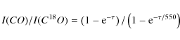
Figure 9 shows the spectrally integrated intensity maps of CO 3-2, HCO+ 4-3 and C18O 3-2 around the position of IRAS 15398-3359. The maps clearly show a single core around the central position, which is completely spatially resolved. There is little to no C18O or HCO+ emission outside of the core, while the CO 3-2 has emission lines at around 10 K in the surrounding cloud. The C18O map, which lacks outflow emission, is somewhat shifted to the south from the other two maps. The spectra at the central source position taken from these maps can be found in Fig. 10. The CO spectra are dominated by the blue-shifted outflow. The integrated intensity of HCO+ 4-3 can be found in Table 4. The independently calibrated CO 3-2 spectra taken with JCMT HARP-B differ from the spectrum taken with APEX-2a by only 3% in integrated intensity, well within the stated calibration uncertainties of both telescopes.
Table 3: 12CO and C18O resultsa.
Table 4: HCO+ and H13CO+ results.
4 Analysis
4.1 Envelope properties
Assuming the (sub-)mm emission is dominated by the cold dust in the
protostellar envelope, its mass can be derived from dust continuum
observations (Shirley et al. 2000; Jørgensen et al. 2002). Using the SCUBA Legacy
archive (Di Francesco et al. 2008), envelope masses were derived for YSOs
in Corona Australis. Henning et al. (1993) observed
fluxes at 1.3 mm for a large sample in Chamaeleon using the SEST,
which are used here to constrain the masses of the very southern
sources. All masses were derived using the relation

|
(1) |
assuming an isothermal sphere of 20 K, a gas-to-dust ratio of 100 and a dust emissivity
![\begin{figure}
\par\includegraphics[width=200pt]{11099f6a.ps}\includegraphics[wi...
...width=200pt]{11099f6e.ps}\includegraphics[width=180pt]{11099f6f.ps}
\end{figure}](/articles/aa/full_html/2009/46/aa11099-08/img45.png)
|
Figure 6:
HCO+ J= 4-3 ( left) and CO 3-2 ( right) maps
of Ced 110 IRS 4 ( top), CrA IRAS 32 ( middle) and HH 100
( bottom). The maps are
|
| Open with DEXTER | |
![\begin{figure}
\par\includegraphics[width=200pt]{11099f7a.ps}\includegraphics[wi...
...width=200pt]{11099f7c.ps}\includegraphics[width=180pt]{11099f7d.ps}
\end{figure}](/articles/aa/full_html/2009/46/aa11099-08/img46.png)
|
Figure 7:
HCO+ J = 4-3 ( left) and CO 3-2 ( right) maps of RCrA IRS 7 ( top) and HH 46 ( bottom). The maps are
|
| Open with DEXTER | |
![\begin{figure}
\par\includegraphics[width=130pt]{11099f8a.ps}\includegraphics[wi...
...width=130pt]{11099f8e.ps}\includegraphics[width=130pt]{11099f8f.ps}
\end{figure}](/articles/aa/full_html/2009/46/aa11099-08/img47.png)
|
Figure 8: CO J= 4-3 integrated intensity maps taken with FLASH of Ced 110 IRS 4, Ced 110 IRS 6 and Cha INa2 ( top row), and Cha IRN, HH 46 and IRAS 12496-7650 ( bottom row). Note that the noise levels in these maps are higher than in the spectra given in Fig. 5. Source positions are marked with ``X''. The APEX beam is shown in the lower right image. The lines are drawn to guide the eye. |
| Open with DEXTER | |
![\begin{figure}
\par\includegraphics[width=400pt]{11099f9.ps}
\end{figure}](/articles/aa/full_html/2009/46/aa11099-08/img48.png)
|
Figure 9: The spectrally integrated intensities of CO 3-2 left, HCO+ 4-3 middle and C18O 3-2 right observed toward IRAS 15398-3359 with HARP-B on the JCMT. Spectra were integrated between velocities of -5 and 15 km s-1. The source itself is at 5.2 km s-1. The cores are all slightly resolved, compared to the 15'' beam of the JCMT. |
| Open with DEXTER | |
![\begin{figure}
\par\includegraphics[width=200pt]{11099f10.ps}
\end{figure}](/articles/aa/full_html/2009/46/aa11099-08/img49.png)
|
Figure 10: The spectra of CO 3-2 top, HCO+ 4-3 middle and C18O 3-2 bottom observed with HARP-B on the JCMT at the central source position. |
| Open with DEXTER | |
Table 5: Overview of the envelope propertiesa.
With the assumption that the H13CO+ 4-3 and C18O 3-2
emission is optically thin, one can estimate the column densities of
these molecules in the protostellar envelope. In this calculation, an
excitation temperature of 20 K is assumed, based on the average
temperature within the protostellar envelope, for both the envelope
and cloud material. Table 5 gives the
column densities of H2, C18O and H13CO+, where the
H2 column density is derived from the C18O column density
assuming a H2/CO ratio of 104 and a 16O/18O ratio of
550 (Wilson & Rood 1994). The H2 column densities range from a few
times 1022 cm-2 in Chamaeleon to a few times 1023 cm-2 in Corona Australis, all in a 18'' beam. However,
freeze-out of CO onto the interstellar grains make the adopted ratio
of H2 over CO a lower limit. In very cold regions (T < 15 K),
abundances can be as much as two orders of magnitude lower than the
assumed CO/H2 abundance of 10-4.
For sources where continuum data at 850 ![]() m are available from
Di Francesco et al. (2008), the column density was independently
calculated from the dust, assuming a dust temperature of 20 K. These
numbers are in general a factor of 2 to 3 higher consistent with some
freeze-out of CO, but for some sources the column densities derived
from the dust approach those obtained from C18O.
m are available from
Di Francesco et al. (2008), the column density was independently
calculated from the dust, assuming a dust temperature of 20 K. These
numbers are in general a factor of 2 to 3 higher consistent with some
freeze-out of CO, but for some sources the column densities derived
from the dust approach those obtained from C18O.
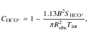
The isotopologue observations of C18O and H13CO+ also
allow to estimate the average optical depth ![]() in the CO 3-2
and HCO+ 4-3 lines (Table 5) following the formula of
in the CO 3-2
and HCO+ 4-3 lines (Table 5) following the formula of
|
(2) |
with the isotopologue ratios for both C18O and H13CO+ taken from Wilson & Rood (1994). For I, the peak temperatures from Tables 3 and 4 were taken to avoid contributions from outflow material. The optical depths range from 25 to a few hundred in the CO 3-2 and from about 0.9 to 16 for the HCO+ 4-3. HCO+ 4-3 is still quite optically thick, even though it is associated with just the envelope. One error in the estimates from the optical depths, may be that the C18O 3-2 and H13CO+ themselves are not optically thin, but have optical depths of a few. In that case, the optical depth of the main isotope would lower as well. However, observations of even rarer isotopologues, such as C17O or HC18O+ would be needed.
Recent C18O 3-2 data of the Ophiuchus cloud show that at many locations throughout L 1688, multiple foreground layers are present providing additional reddening of embedded sources (van Kempen et al. 2009b). In our sample, all C18O 3-2 lines can be fitted with single Gaussians indicating that no fore-ground layers are present in any of the observed clouds, in contrast with Ophiuchus.
4.2 Embedded or not?
Analysis of the physical structure of several sources classified as Class I based on their IR spectral slope has shown that some of them are in fact not embedded sources, but rather edge-on disks, such as CRBR 2422.8 (Brandner et al. 2000; Pontoppidan et al. 2005), or IRS 46 (Lahuis et al. 2006). Others turn out to be obscured (background) sources or occasionally even disks in front of a dense core (van Kempen et al. 2009b). Theoretical models from Robitaille et al. (2006) and Crapsi et al. (2008) indeed show that edge-on disks can masquerade as embedded sources in their infrared SED due to the increased reddening.
Following Robitaille et al. (2006) and Crapsi et al. (2008), the border
between a truly embedded so-called ``Stage 1'' source and a ``Stage 2''
star + disk system is put at accretion rates of 10-6 ![]() yr-1, which in the context of these models corresponds to an envelope mass of
yr-1, which in the context of these models corresponds to an envelope mass of ![]() 0.1
0.1 ![]() or a H2 column of
or a H2 column of
![]() cm-2. Because of potential confusion with surrounding
(foreground) clouds and disks, one cannot simply use the masses
derived from the continuum data but one must look in more detail at
the properties of a source. One of the key additional criteria for
identification as a truly embedded source is the concentration of warm
dense gas around the source. The concentration is determined by the
comparison of the peak intensity in a map with the amount of extended
emission. Such a parameter has been extensively discussed and
successfully applied in the analysis of submillimeter continuum
observations from SCUBA (Johnstone et al. 2001;
Walawender et al. 2005; Jørgensen et al. 2007). For example, they have shown that pre-stellar cores have much more extended and less concentrated
emission than protostellar envelopes.
cm-2. Because of potential confusion with surrounding
(foreground) clouds and disks, one cannot simply use the masses
derived from the continuum data but one must look in more detail at
the properties of a source. One of the key additional criteria for
identification as a truly embedded source is the concentration of warm
dense gas around the source. The concentration is determined by the
comparison of the peak intensity in a map with the amount of extended
emission. Such a parameter has been extensively discussed and
successfully applied in the analysis of submillimeter continuum
observations from SCUBA (Johnstone et al. 2001;
Walawender et al. 2005; Jørgensen et al. 2007). For example, they have shown that pre-stellar cores have much more extended and less concentrated
emission than protostellar envelopes.
A recent survey of Class I sources in the Ophiuchus L 1688 region has demonstrated that such a method can be expanded to molecular line mapping and be used as a powerful tool for identifying truly embedded protostars from edge-on disks and obscured sources (van Kempen et al. 2009b). HCO+ 4-3, a high density tracer, proved to be particularly useful. The recipe for proper identification consists of three ingredients. First the peak intensity of HCO+ line should be brighter than 0.4 K, a factor of 4 more than is commonly seen for disks (Thi et al. 2004). Second, the concentration parameter of HCO+4-3 should be higher than 0.6. Third, the HCO+ should preferably be extended within the single dish beam. For non-resolved HCO+emission, other information, such as whether or not the source is extended in the submillimeter continuum or whether it has a (compact) outflow, should be taken into account.
The concentration of HCO+ is defined as:
|
(3) |
with
Table 6: HCO+ 4-3 and CO 4-3 core radii and concentrations.
Table 6 lists the derived concentration parameters
for our sources. Of the 12 sources for which such data exist, 6 have
concentrations of ![]() 0.7 and higher, as well as strong HCO+fluxes above 0.5 K km s-1
associated with the sources,
characteristic of embedded sources. Three sources (HH 100,
IRAS 07178-4429 and IRAS 13546-3941) have no associated HCO+core and thus no concentration.
Similarly, Cha INa2 shows no signs of centrally concentrated CO 4-3
emission. Cha IRS 6a, Cha INa2, RCrA TS 3.5, IRAS 07178-4429 and IRAS 13546-3941 all lack HCO+ 4-3 emission, even below the limit adopted from
Thi et al. (2004), and are thus very likely not embedded YSOs.
0.7 and higher, as well as strong HCO+fluxes above 0.5 K km s-1
associated with the sources,
characteristic of embedded sources. Three sources (HH 100,
IRAS 07178-4429 and IRAS 13546-3941) have no associated HCO+core and thus no concentration.
Similarly, Cha INa2 shows no signs of centrally concentrated CO 4-3
emission. Cha IRS 6a, Cha INa2, RCrA TS 3.5, IRAS 07178-4429 and IRAS 13546-3941 all lack HCO+ 4-3 emission, even below the limit adopted from
Thi et al. (2004), and are thus very likely not embedded YSOs.
HH 100 is an exception. Although no concentration could be calculated
for this source as it is not peaking on the HH 100 source position, there is strong extended HCO+ emission with at least 7![]() ,
and in some areas up to 50
,
and in some areas up to 50![]() .
A
clear outflow is seen in the CO emission in Fig. 6,
thus indicating that HH 100 is an embedded source. This is confirmed
from results from Spitzer-IRAC and MIPS (Peterson, priv. comm.).
However, the lack of concentration from an envelope is puzzling due to
the low optical depth derived for this line at HH100-OFF.
.
A
clear outflow is seen in the CO emission in Fig. 6,
thus indicating that HH 100 is an embedded source. This is confirmed
from results from Spitzer-IRAC and MIPS (Peterson, priv. comm.).
However, the lack of concentration from an envelope is puzzling due to
the low optical depth derived for this line at HH100-OFF.
The RCrA IRS 7 binary system was classified as two embedded sources by Groppi et al. (2007). The elongated HCO+ spatial emission profile indeed suggests that two envelopes are located close to each other. The concentrations of 0.68 and 0.66 (close to 0.7) together with the strong outflow confirm that both sources are embedded. Similar arguments are used to classify RCrA IRS5 and IRAS 12496-7650 as embedded YSOs. In summary, using our line diagnostics, we have confirmed that eleven of our sixteen Class I sources are truly embedded YSOs, and five sources very likely not.
4.3 Outflows
4.3.1 Temperatures
If we assume that these line wings fill the beam and are tracing the dominant part of the outflowing gas mass (also known as the swept up gas), then the ratios of emission in the line wings of the CO 3-2, 4-3 and 7-6 profiles at the central position in Table 7 can be compared to model line ratios from Appendix C of van der Tak et al. (2007), derived using statistical equilibrium calculations within an escape probability formalism. The line wings are assumed to be optically thin and filling factors to be the same within the different beams. A quick look at the line wings of CO 3-2 and C18O 3-2 in the sources in Corona Australis provides an upper limit to the optical depth of the CO line wing of about 3.1 close to the quiescent part of the line. At more extreme velocities, the opacity is probably much lower and indeed optically thin. Optically thin line wings were also shown to be a good assumption for the case of HH 46 by van Kempen et al. (2009a). Kinetic temperatures can then be derived if outflow emission is detected in two of these three lines. Note that an observed ratio leads to a degenerate solution of the kinetic temperature and local density and not a unique solution of the temperature. Thus, some estimate of the local density must be available. Densities in the outer envelope can be estimated from radiative transfer modelling of the dust continuum emission and SED (Ivezic & Elitzur 1997). H2 densities of a few times 105 cm-3 are derived by Jørgensen et al. (2002) for distances of 1500-3000 AU (corresponding to 10-20'' at the distances of Chamaeleon and Corona Australis), but these drop to a few times 104 cm-3 at a few thousand AU. These densities are assumed to be comparable to the densities in the swept-up gas at these distances.
Table 7: Temperature constraints of CO line wings ratiosd.
Table 8: Outflow parameters from the CO 3-2 mapping.
At densities above the critical density,
![]() cm-3 for CO 3-2, the gas is
thermally excited and a temperature can be inferred directly. For
lower densities, the gas is subthermally excited and higher kinetic
temperatures are needed to produce similar ratios of the line wings.
To estimate the temperatures, two scenarios are presented. In the
first, it is assumed that the gas is thermally excited (
cm-3 for CO 3-2, the gas is
thermally excited and a temperature can be inferred directly. For
lower densities, the gas is subthermally excited and higher kinetic
temperatures are needed to produce similar ratios of the line wings.
To estimate the temperatures, two scenarios are presented. In the
first, it is assumed that the gas is thermally excited (
![]() )
since densities in the envelope are near to, or higher
than, the CO 3-2 critical density. This is applicable for all sources
with the exception of HH 46, for which the central beam extends to
about 4500 AU in radius. The kinetic temperatures determined in this
way are lower limits. A second scenario is considered by assuming
that the densities are of order 104 cm-3,
closer to typical
densities of the surrounding cloud or envelopes at larger radii. In
the first scenario, outflow temperatures are on the order of 50 K.
An exception is IRAS 15398-3359, which appears to be much
warmer (100 K) from both the CO 3-2/4-3 ratio as well as the
4-3/7-6 ratio in the blue outflow. Since we lack CO 4-3 and/or 7-6
data of the red outflow, no temperature could be determined for the
red outflow. If densities are lower (scenario 2), derived kinetic
temperatures are on the order of 150 K, although for HH 46
(blue) and
Ced 110 IRS 6 (both red and blue) the outflow temperatures
are
consistent with
)
since densities in the envelope are near to, or higher
than, the CO 3-2 critical density. This is applicable for all sources
with the exception of HH 46, for which the central beam extends to
about 4500 AU in radius. The kinetic temperatures determined in this
way are lower limits. A second scenario is considered by assuming
that the densities are of order 104 cm-3,
closer to typical
densities of the surrounding cloud or envelopes at larger radii. In
the first scenario, outflow temperatures are on the order of 50 K.
An exception is IRAS 15398-3359, which appears to be much
warmer (100 K) from both the CO 3-2/4-3 ratio as well as the
4-3/7-6 ratio in the blue outflow. Since we lack CO 4-3 and/or 7-6
data of the red outflow, no temperature could be determined for the
red outflow. If densities are lower (scenario 2), derived kinetic
temperatures are on the order of 150 K, although for HH 46
(blue) and
Ced 110 IRS 6 (both red and blue) the outflow temperatures
are
consistent with ![]() 80 K.
Errors on the outflow temperatures are generally on the order of 25 to
40%, due to the sensitive dependency on density, as well as errors on
the estimate of the CO line ratios.
80 K.
Errors on the outflow temperatures are generally on the order of 25 to
40%, due to the sensitive dependency on density, as well as errors on
the estimate of the CO line ratios.
Bow-shock driven shell models by Hatchell et al. (1999) predict
temperatures of the swept-up gas by calculating the energy balance
between the heating due to the kinetic energy of the expanding
momentum-conserving shell and the line cooling of the gas. For
parameters typical of the Class 0 L 483 source (
![]() ,
,
![]() ), outflow temperatures of 50 to 100 K
are found in the inner few thousand AU from the star. Along the bulk
of the outflow axis, temperatures are modelled to be 100-150 K.
Higher temperatures in excess of a few hundred to a thousand K are
predicted only near the bow shocks. The models depend on the local
conditions such as dust cooling, density distribution and jet
velocity, but most parameters have an influence of the order of a few
tens of K on the temperature along most of the outflow. The results
in Table 7 agree well with the temperature
predictions from Hatchell et al. (1999) and suggest that jet velocities
>100 km s-1 are not present, with the exception of IRAS 15398-3359.
), outflow temperatures of 50 to 100 K
are found in the inner few thousand AU from the star. Along the bulk
of the outflow axis, temperatures are modelled to be 100-150 K.
Higher temperatures in excess of a few hundred to a thousand K are
predicted only near the bow shocks. The models depend on the local
conditions such as dust cooling, density distribution and jet
velocity, but most parameters have an influence of the order of a few
tens of K on the temperature along most of the outflow. The results
in Table 7 agree well with the temperature
predictions from Hatchell et al. (1999) and suggest that jet velocities
>100 km s-1 are not present, with the exception of IRAS 15398-3359.
Although we assumed the line wings to be optically thin, this is not necessarily the case (e.g., Cabrit & Bertout 1992; Hogerheijde et al. 1998). A more in-depth discussion of the effects of optical depth and density on the kinetic temperatures of the swept-up gas in the molecular outflow of HH 46 IRS is presented in van Kempen et al. (2009a). A lower line ratio for the same temperature can also be caused by a higher optical depth in one of the line wings. Similarly a higher density will lead to lower inferred temperatures for the same observed line ratio. Hatchell et al. (1999) also show that there may be a temperature gradient away from the connecting line between bow shock and origin at the protostar. However, this gradient is often diluted out and may be observable within a single beam. The different temperatures of two different ratios may be responsible for this.
![\begin{figure}
\par\includegraphics[width=450pt]{11099f13.ps}
\end{figure}](/articles/aa/full_html/2009/46/aa11099-08/img80.png)
|
Figure 11:
CO outflow force
|
| Open with DEXTER | |
4.3.2 Other outflow parameters
For the six sources where outflow emission has been mapped in
12CO 3-2, it is possible to determine the spatial outflow
parameters, such as outflow mass, maximum velocity and
extent. Subsequently the dynamical time scales and average mass
outflow rate, the outflow force (or momentum flux) and kinetic
luminosity can be derived following a recipe detailed in
Hogerheijde et al. (1998) with the assumption that the emission at the
more extreme velocities is optically thin and that the material has
kinetic temperatures of 50-80 K. For IRAS 15398-3359 a
temperature of 100 K is adopted. The inclination of the outflow with
the plane of the sky influences the results and the derived values
need to be corrected for their inclination using an average of the
model predictions in Cabrit & Bertout (1990). For HH 46 the inclination has
been constrained to 35![]() (Reipurth & Heathcote 1991; Micono et al. 1998). For the
other sources, an inclination is estimated from the distance between
the major and minor axes of the maximum contour levels in
Figs. 6 and 7 (see Table 8).
(Reipurth & Heathcote 1991; Micono et al. 1998). For the
other sources, an inclination is estimated from the distance between
the major and minor axes of the maximum contour levels in
Figs. 6 and 7 (see Table 8).
The results in Table 8 show that most outflows have
masses of 0.01-0.1 ![]() ,
with average mass loss rates between
,
with average mass loss rates between
![]() to
to
![]() yr-1, and
outflow forces
yr-1, and
outflow forces
![]() of
of
![]() to
to
![]() yr-1 km s-1. The strongest
outflow is RCrA IRS 7, which produces the highest outflow force and
the most kinetic luminosity. This is mainly caused by the fact that emission
is detected out to
yr-1 km s-1. The strongest
outflow is RCrA IRS 7, which produces the highest outflow force and
the most kinetic luminosity. This is mainly caused by the fact that emission
is detected out to
![]() as high as 23 km s-1, compared
with 4 to 9 km s-1
for the other sources, almost an order of
magnitude difference. Note that for HH 100 (red only), HH 46
(red
only) and RCrA IRS 7 (red and blue), the quoted outflow radius is a
lower limit, due to insufficient coverage. The resulting outflow force
and kinetic luminosity are thus upper limits. For HH 100 and and
RCrA IRS 7 subtracting Gaussians with widths of 3 km s-1 changes the
integrated intensity by 20
as high as 23 km s-1, compared
with 4 to 9 km s-1
for the other sources, almost an order of
magnitude difference. Note that for HH 100 (red only), HH 46
(red
only) and RCrA IRS 7 (red and blue), the quoted outflow radius is a
lower limit, due to insufficient coverage. The resulting outflow force
and kinetic luminosity are thus upper limits. For HH 100 and and
RCrA IRS 7 subtracting Gaussians with widths of 3 km s-1 changes the
integrated intensity by 20![]() .
All other parameters depend linearly
on the mass M that is derived from the integrated intensity.
.
All other parameters depend linearly
on the mass M that is derived from the integrated intensity.
Hogerheijde et al. (1998) surveyed the outflows of Class I sources in the
Taurus cloud. There, most sources produce weaker outflows than found
in Table 8, with outflow forces of the order of a
few times 10
![]() yr-1 km s-1, with a few sources having values as high a few times 10
yr-1 km s-1, with a few sources having values as high a few times 10
![]() yr-1 km s-1.
A recent survey of the outflows present in the Perseus cloud shows
yr-1 km s-1.
A recent survey of the outflows present in the Perseus cloud shows
![]() values of a few times 10
values of a few times 10
![]() yr-1 km s-1 to a few times
yr-1 km s-1 to a few times
![]() yr-1 km s-1(Hatchell et al. 2007a).
However, these numbers were not corrected for
inclination, which can account for at least a factor of
5 increase. The observed outflow forces in our sample are all
among the
upper range of these values, especially HH 100 and RCrA IRS
7. Figure
5 of Hatchell et al. (2007a) shows that most Class I outflows have lower
outflow forces than the Class 0 sources.
yr-1 km s-1(Hatchell et al. 2007a).
However, these numbers were not corrected for
inclination, which can account for at least a factor of
5 increase. The observed outflow forces in our sample are all
among the
upper range of these values, especially HH 100 and RCrA IRS
7. Figure
5 of Hatchell et al. (2007a) shows that most Class I outflows have lower
outflow forces than the Class 0 sources.
Most flows observed from the northern hemisphere were first
discussed in Bontemps et al. (1996) using CO 2-1 observations with
relatively large beams. Outflow forces range from a few times
10-7 to 10
![]() yr-1 km s-1, corrected for
inclination and optical depth. In Bontemps et al. (1996), a relation between the
outflow forces, bolometric luminosities and envelope masses was
empirically derived,
yr-1 km s-1, corrected for
inclination and optical depth. In Bontemps et al. (1996), a relation between the
outflow forces, bolometric luminosities and envelope masses was
empirically derived,
![]() and
and
![]() .
Figure 11 shows a comparison between the observed
outflows of Table 8 and the relations from
Bontemps et al. (1996). Although the
outflows in our sample are all associated with Class I sources,
they are exceptionally strong outflows for their luminosity, but not
for their envelope mass. Outflow forces are one to two orders of
magnitude
higher than expected from the above equation with luminosity. This
suggests that the outflow
strength as measured through the swept-up material says more about the
surroundings (i.e., the amount of matter that can be swept up) than
about the intrinsic source and outflow properties.
.
Figure 11 shows a comparison between the observed
outflows of Table 8 and the relations from
Bontemps et al. (1996). Although the
outflows in our sample are all associated with Class I sources,
they are exceptionally strong outflows for their luminosity, but not
for their envelope mass. Outflow forces are one to two orders of
magnitude
higher than expected from the above equation with luminosity. This
suggests that the outflow
strength as measured through the swept-up material says more about the
surroundings (i.e., the amount of matter that can be swept up) than
about the intrinsic source and outflow properties.
4.3.3 The outflow of IRAS 12496-7650
An outflow was identified from the line profiles in van Kempen et al. (2006) and it was concluded that the emission as seen with ISO-LWS (Giannini et al. 2001) has to originate on scales larger than 8'' and not from the inner regions of a protostellar envelope around IRAS 12496-7650. Figure 12 reveals that the detected blue-shifted outflow is located only in the central 15'' and is peaking strongly on the source. The lack of red-shifted emission reinforces the conclusion that the outflowing gas is viewed almost perfectly face-on and that our line of sight is straight down the outflow cone.
![\begin{figure}
\par\includegraphics[width=240pt]{11099f11.ps}
\end{figure}](/articles/aa/full_html/2009/46/aa11099-08/img91.png)
|
Figure 12: CO J=4-3 map of IRAS 12496-7650. The blue and red-shifted outflow emission are shown in solid and dashed contours respectively in steps of 10% of the maximum of 34.8 K km s-1. |
| Open with DEXTER | |
4.3.4 The outflow of IRAS 15398-3359
The line profiles of IRAS 15398-3359 have a clear blue outflow
component, with red-shifted emission notseen until further off source.
If only the line wings are mapped, Figure 13 shows
that the outflow of IRAS 15398-3359 is small and extends only
![]() 25'' across the sky. As discussed above, the blue part of the outflow is exceptionally
warm, with significant outflow emission seen in the CO 7-6
line. Although it is smaller in extent, the outflow does not stand out
w.r.t to the others in terms of outflow properties as measured from
their CO 3-2 maps.
25'' across the sky. As discussed above, the blue part of the outflow is exceptionally
warm, with significant outflow emission seen in the CO 7-6
line. Although it is smaller in extent, the outflow does not stand out
w.r.t to the others in terms of outflow properties as measured from
their CO 3-2 maps.
![\begin{figure}
\par\hspace*{-3mm}\includegraphics[width=240pt]{11099f12.ps}
\vspace*{8mm}
\end{figure}](/articles/aa/full_html/2009/46/aa11099-08/img92.png)
|
Figure 13:
CO J=3-2 map of IRAS 15398-3359. The blue and red-shifted
outflow emission are shown in blue and red
contours
respectively in steps of 10% of the maximum of
8.1 K km s-1. The grey-scale and dashed contour lines in
the background are the
850 |
| Open with DEXTER | |
5 Conclusions
We present observations of CO, HCO+ and their isotopologues, ranging in excitation from CO 3-2 to CO 7-6 of a sample of southern embedded sources to probe the molecular gas content in both the protostellar envelopes and molecular outflows in preparation for future ALMA and Herschel surveys. The main conclusions are the following:
- HCO+ 4-3 and CO 4-3 integrated intensities and concentrations, combined with information on the presence of outflows, confirm the presence of warm dense quiescent gas associated with 11 of our 16 sources.
- RCrA TS 3.5, Cha IRS 6a, Cha INa2, IRAS 07178-4429 and IRAS 13546-3941 are likely not embedded YSOs due to the lack of HCO+ 4-3 emission and/or the lack of central concentration in HCO+ 4-3.
- The swept-up outflow gas has temperatures of the order of 50-100 K, as measured from the ratios of the CO line profile wings, with the values depending on the adopted ambient densities. These values are comparable to the temperatures predicted by the heating model of Hatchell et al. (1999), with the exception of IRAS 15398-3359, which may be unusually warm.
- The outflows of 6 of our truly embedded sources - Ced 110 IRS 4, CrA IRAS 32, RCrA IRS 7A, HH 100, HH 46, IRAS 15398-3359 - were characterized using CO spectral maps. The outflows all have exceptionally strong outflow forces, almost two orders of magnitude higher than expected from their luminosities following the relation of Bontemps et al. (1996).
- Neither Chamaeleon nor Corona Australis have foreground layers as found in Ophiuchus L 1688. All C18O 3-2 spectra can be fitted with single Gaussians.
TvK and astrochemistry at Leiden Observatory are supported by a Spinoza prize and by NWO grant 614.041.004. The APEX staff, in particular Michael Dumke, are thanked for their extensive support and carrying out the observations. We are also grateful for the constructive comments of the anonymous referee.
References
- André, P., Ward-Thompson, D., & Barsony, M. 1993, ApJ, 406, 122 [NASA ADS] [CrossRef]
- Bachiller, R., & Tafalla, M. 1999, in The Origin of Stars and Planetary Systems, ed. C. J. Lada, & N. D. Kylafis (Dordrecht: Kluwer), 227
- Belloche, A., Parise, B., van der Tak, F. F. S., et al. 2006, A&A, 454, L51 [NASA ADS] [CrossRef] [EDP Sciences]
- Blake, G. A., van Dishoek, E. F., Jansen, D. J., Groesbeck, T. D., & Mundy, L. G. 1994, ApJ, 428, 680 [NASA ADS] [CrossRef]
- Bontemps, S., Andre, P., Terebey, S., et al. 1996, A&A, 311, 858 [NASA ADS]
- Boogert, A. C. A., Hogerheijde, M. R., Ceccarelli, C., et al. 2002, ApJ, 570, 708 [NASA ADS] [CrossRef]
- Bourke, T. L., Hyland, A. R., & Robinson, G. 1995, MNRAS, 276, 1052 [NASA ADS]
- Brandner, W., Sheppard, S., Zinnecker, H., et al. 2000, A&A, 364, L13 [NASA ADS]
- Brown, A. 1987, ApJ, 322, L31 [NASA ADS] [CrossRef]
- Cabrit, S., & Bertout, C. 1990, ApJ, 348, 530 [NASA ADS] [CrossRef]
- Cabrit, S., & Bertout, C. 1992, A&A, 261, 274 [NASA ADS]
- Chernin, L. M., & Masson, C. R. 1991, ApJ, 382, L93 [NASA ADS] [CrossRef]
- Chini, R., Kämpgen, K., Reipurth, B., et al. 2003, A&A, 409, 235 [NASA ADS] [CrossRef] [EDP Sciences]
- Crapsi, A., van Dishoeck, E. F., Hogerheijde, M. R., Pontoppidan, K. M., & Dullemond, C. P. 2008, A&A, 486, 245 [NASA ADS] [CrossRef] [EDP Sciences]
- Damjanov, I., Jayawardhana, R., Scholz, A., et al. 2007, ApJ, 670, 1337 [NASA ADS] [CrossRef]
- Di Francesco, J., Johnstone, D., Kirk, H., MacKenzie, T., & Ledwosinska, E. 2008, ApJS, 175, 277 [NASA ADS] [CrossRef]
- Evans, N. J., Allen, L. E., Blake, G. A., et al. 2003, PASP, 115, 965 [NASA ADS] [CrossRef]
- Evans, II, N. J., Lee, J.-E., Rawlings, J. M. C., et al. 2005, ApJ, 626, 919 [NASA ADS] [CrossRef]
- Evans, II, N. J., Dunham, M. M., Jørgensen, J. K., et al. 2009, ApJ, in press
- Froebrich, D. 2005, ApJS, 156, 169 [NASA ADS] [CrossRef]
- Giannini, T., Lorenzetti, D., Tommasi, E., et al. 1999, A&A, 346, 617 [NASA ADS]
- Giannini, T., Nisini, B., & Lorenzetti, D. 2001, ApJ, 555, 40 [NASA ADS] [CrossRef]
- Groppi, C. E., Hunter, T. R., Blundell, R., et al. 2007, ApJ, 670, 489 [NASA ADS] [CrossRef]
- Güsten, R., Nyman, L. Å., Schilke, P., et al. 2006, A&A, 454, L13 [NASA ADS] [CrossRef] [EDP Sciences]
- Gutermuth, R. A., Myers, P. C., Megeath, S. T., et al. 2008, ApJ, 674, 336 [NASA ADS] [CrossRef]
- Haikala, L. K., Juvela, M., Harju, J., et al. 2006, A&A, 454, L71 [NASA ADS] [CrossRef] [EDP Sciences]
- Harju, J., Haikala, L. K., Mattila, K., et al. 1993, A&A, 278, 569 [NASA ADS]
- Hartmann, L., Megeath, S. T., Allen, L., et al. 2005, ApJ, 629, 881 [NASA ADS] [CrossRef]
- Hatchell, J., Fuller, G. A., & Ladd, E. F. 1999, A&A, 344, 687 [NASA ADS]
- Hatchell, J., Fuller, G. A., & Richer, J. S. 2007a, A&A, 472, 187 [NASA ADS] [CrossRef] [EDP Sciences]
- Hatchell, J., Fuller, G. A., Richer, J. S., Harries, T. J., & Ladd, E. F. 2007b, A&A, 468, 1009 [NASA ADS] [CrossRef] [EDP Sciences]
- Heathcote, S., Morse, J. A., Hartigan, P., et al. 1996, AJ, 112, 1141 [NASA ADS] [CrossRef]
- Henning, T., Pfau, W., Zinnecker, H., et al. 1993, A&A, 276, 129 [NASA ADS]
- Heyminck, S., Kasemann, C., Güsten, R., de Lange, G., & Graf, U. U. 2006, A&A, 454, L21 [NASA ADS] [CrossRef] [EDP Sciences]
- Hiramatsu, M., Hayakawa, T., Tatematsu, K., et al. 2007, ApJ, 664, 964 [NASA ADS] [CrossRef]
- Hogerheijde, M. R., van Dishoeck, E. F., Blake, G. A., et al. 1997, ApJ, 489, 293 [NASA ADS] [CrossRef]
- Hogerheijde, M. R., van Dishoeck, E. F., Blake, G. A., et al. 1998, ApJ, 502, 315 [NASA ADS] [CrossRef]
- Hughes, J., & Hartigan, P. 1992, AJ, 104, 680 [NASA ADS] [CrossRef]
- Ivezic, Z., & Elitzur, M. 1997, MNRAS, 287, 799 [NASA ADS]
- Johnstone, D., Wilson, C. D., Moriarty-Schieven, G., et al. 2000, ApJ, 545, 327 [NASA ADS] [CrossRef]
- Johnstone, D., Fich, M., Mitchell, G. F., et al. 2001, ApJ, 559, 307 [NASA ADS] [CrossRef]
- Jørgensen, J. K., Schöier, F. L., & van Dishoeck, E. F. 2002, A&A, 389, 908 [NASA ADS] [CrossRef] [EDP Sciences]
- Jørgensen, J. K., Lahuis, F., Schöier, F. L., et al. 2005a, ApJ, 631, L77 [NASA ADS] [CrossRef]
- Jørgensen, J. K., Schöier, F. L., & van Dishoeck, E. F. 2005b, A&A, 437, 501 [NASA ADS] [CrossRef] [EDP Sciences]
- Jørgensen, J. K., Bourke, T. L., Myers, P. C., et al. 2007, ApJ, 659, 479 [NASA ADS] [CrossRef]
- Klein, B., Philipp, S. D., Krämer, I., et al. 2006, A&A, 454, L29 [NASA ADS] [CrossRef] [EDP Sciences]
- Knude, J., & Høg, E. 1998, A&A, 338, 897 [NASA ADS]
- Lada, C. J. 1987, in Star Forming Regions, ed. M. Peimbert, J. Jugaku, & P. W. J. L. Brand (Reidel, Dordrecht), IAU Symp., 115, 1
- Lahuis, F., van Dishoeck, E. F., Boogert, A. C. A., et al. 2006, ApJ, 636, L145 [NASA ADS] [CrossRef]
- Lehtinen, K., Haikala, L. K., Mattila, K., et al. 2001, A&A, 367, 311 [NASA ADS] [CrossRef] [EDP Sciences]
- Leurini, S., Schilke, P., Menten, K. M., et al. 2004, A&A, 422, 573 [NASA ADS] [CrossRef] [EDP Sciences]
- Loren, R. B. 1979, ApJ, 227, 832 [NASA ADS] [CrossRef]
- Luhman, K. L., & Rieke, G. H. 1999, ApJ, 525, 440 [NASA ADS] [CrossRef]
- Luhman, K. L., Allen, L. E., Allen, P. R., et al. 2008, ApJ, 675, 1375 [NASA ADS] [CrossRef]
- Maheswar, G., Manoj, P., & Bhatt, H. C. 2004, MNRAS, 355, 1272 [NASA ADS] [CrossRef]
- Mangum, J. G., & Wootten, A. 1993, ApJS, 89, 123 [NASA ADS] [CrossRef]
- Maret, S., Ceccarelli, C., Caux, E., et al. 2004, A&A, 416, 577 [NASA ADS] [CrossRef] [EDP Sciences]
- Micono, M., Davis, C. J., Ray, T. P., Eisloeffel, J., & Shetrone, M. D. 1998, ApJ, 494, L227 [NASA ADS] [CrossRef]
- Motte, F., Andre, P., & Neri, R. 1998, A&A, 336, 150 [NASA ADS]
- Murphy, D. C., Cohen, R., & May, J. 1986, A&A, 167, 234 [NASA ADS]
- Nisini, B., Antoniucci, S., Giannini, T., et al. 2005, A&A, 429, 543 [NASA ADS] [CrossRef] [EDP Sciences]
- Noriega-Crespo, A., Morris, P., Marleau, F. R., et al. 2004, ApJS, 154, 352 [NASA ADS] [CrossRef]
- Nutter, D. J., Ward-Thompson, D., & André, P. 2005, MNRAS, 357, 975 [NASA ADS] [CrossRef]
- Nutter, D., Kirk, J. M., Stamatellos, D., et al. 2008, MNRAS, 384, 755 [NASA ADS] [CrossRef]
- Olofsson, G., Huldtgren, M., Kaas, A. A., et al. 1999, A&A, 350, 883 [NASA ADS]
- Ossenkopf, V., & Henning, T. 1994, A&A, 291, 943 [NASA ADS]
- Parise, B., Belloche, A., Leurini, S., et al. 2006, A&A, 454, L79 [NASA ADS] [CrossRef] [EDP Sciences]
- Persi, P., Marenzi, A. R., Kaas, A. A., et al. 1999, AJ, 117, 439 [NASA ADS] [CrossRef]
- Persi, P., Marenzi, A. R., Olofsson, G., et al. 2000, A&A, 357, 219 [NASA ADS]
- Persi, P., Marenzi, A. R., Gómez, M., et al. 2001, A&A, 376, 907 [NASA ADS] [CrossRef] [EDP Sciences]
- Pontoppidan, K. M., Fraser, H. J., Dartois, E., et al. 2003, A&A, 408, 981 [NASA ADS] [CrossRef] [EDP Sciences]
- Pontoppidan, K. M., Dullemond, C. P., van Dishoeck, E. F., et al. 2005, ApJ, 622, 463 [NASA ADS] [CrossRef]
- Reipurth, B., & Heathcote, S. 1991, A&A, 246, 511 [NASA ADS]
- Risacher, C., Vassilev, V., Monje, R., et al. 2006, A&A, 454, L17 [NASA ADS] [CrossRef] [EDP Sciences]
- Robitaille, T. P., Whitney, B. A., Indebetouw, R., Wood, K., & Denzmore, P. 2006, ApJS, 167, 256 [NASA ADS] [CrossRef]
- Santos, N. C., Yun, J. L., Santos, C. A., et al. 1998, AJ, 116, 1376 [NASA ADS] [CrossRef]
- Schöier, F. L., Jørgensen, J. K., van Dishoeck, E. F., et al. 2002, A&A, 390, 1001 [NASA ADS] [CrossRef] [EDP Sciences]
- Schöier, F. L., Jørgensen, J. K., Pontoppidan, K. M., & et al. 2006, A&A, 454, L67 [NASA ADS] [CrossRef] [EDP Sciences]
- Shirley, Y. L., Evans, N. J., Rawlings, J. M. C., et al. 2000, ApJS, 131, 249 [NASA ADS] [CrossRef]
- Shirley, Y. L., Evans, II, N. J., & Rawlings, J. M. C. 2002, ApJ, 575, 337 [NASA ADS] [CrossRef]
- Snell, R. L., Dickman, R. L., & Huang, Y.-L. 1990, ApJ, 352, 139 [NASA ADS] [CrossRef]
- Stanke, T., McCaughrean, M. J., & Zinnecker, H. 1999, A&A, 350, L43 [NASA ADS]
- Stanke, T., Smith, M. D., Gredel, R., et al. 2006, A&A, 447, 609 [NASA ADS] [CrossRef] [EDP Sciences]
- Taylor, K. N. R., & Storey, J. W. V. 1984, MNRAS, 209, 5P [NASA ADS]
- Thi, W.-F., van Zadelhoff, G.-J., & van Dishoeck, E. F. 2004, A&A, 425, 955 [NASA ADS] [CrossRef] [EDP Sciences]
- van der Tak, F. F. S., van Dishoeck, E. F., Evans, N. J., et al. 2000, ApJ, 537, 283 [NASA ADS] [CrossRef]
- van der Tak, F. F. S., Black, J. H., Schöier, F. L., Jansen, D. J., & van Dishoeck, E. F. 2007, A&A, 468, 627 [NASA ADS] [CrossRef] [EDP Sciences]
- van Dishoeck, E. F., Blake, G. A., Jansen, D. J., et al. 1995, ApJ, 447, 760 [NASA ADS] [CrossRef]
- van Kempen, T. A., Hogerheijde, M. R., van Dishoeck, E. F., et al. 2006, A&A, 454, L75 [NASA ADS] [CrossRef] [EDP Sciences]
- van Kempen, T. A., van Dishoeck, E. F., Güsten, R., et al. 2009a, A&A, 501, 633 [NASA ADS] [CrossRef] [EDP Sciences]
- van Kempen, T. A., van Dishoeck, E. F., Salter, D. M., et al. 2009b, A&A, 498, 167 [NASA ADS] [CrossRef] [EDP Sciences]
- Velusamy, T., Langer, W. D., & Marsh, K. A. 2007, ApJ, 668, L159 [NASA ADS] [CrossRef]
- Walawender, J., Bally, J., Kirk, H., et al. 2005, AJ, 130, 1795 [NASA ADS] [CrossRef]
- Wilking, B. A., Taylor, K. N. R., & Storey, J. W. V. 1986, AJ, 92, 103 [NASA ADS] [CrossRef]
- Wilking, B. A., McCaughrean, M. J., Burton, M. G., et al. 1997, AJ, 114, 2029 [NASA ADS] [CrossRef]
- Wilson, T. L., & Rood, R. 1994, ARA&A, 32, 191 [NASA ADS] [CrossRef]
- Young, C. H., Shirley, Y. L., Evans, II, N. J., et al. 2003, ApJS, 145, 111 [NASA ADS] [CrossRef]
Footnotes
- ...(Güsten et al. 2006)
![[*]](/icons/foot_motif.png)
- This publication is based on data acquired with the Atacama Pathfinder Experiment (APEX) with programs E-77.C-0217, E-77.C-4010 and E-78.C-0576. APEX is a collaboration between the Max-Planck-Institut für Radioastronomie, the European Southern Observatory, and the Onsala Space Observatory.
- ... telescope (JCMT)
- The James Clerk Maxwell Telescope is operated by The Joint Astronomy Centre on behalf of the Science and Technology Facilities Council of the United Kingdom, the Netherlands Organisation for Scientific Research, and the National Research Council of Canada. Data were obtained with programs M06BN11, M07BN09 and M08AN05.
- ... HARP4
- See JCMT website http://www.jcmt.jach.hawaii.edu/
- ... package
- CLASS is part of the GILDAS reduction package. See http://www.iram.fr/IRAMFR/GILDAS for more information.
All Tables
Table 1: Source sample.
Table 2: Overview of the APEX observations.
Table 3: 12CO and C18O resultsa.
Table 4: HCO+ and H13CO+ results.
Table 5: Overview of the envelope propertiesa.
Table 6: HCO+ 4-3 and CO 4-3 core radii and concentrations.
Table 7: Temperature constraints of CO line wings ratiosd.
Table 8: Outflow parameters from the CO 3-2 mapping.
All Figures
|
|
Figure 1: 12CO 3-2 spectra of the sources in Chamaeleon ( far left) and Corona Australis ( middle left) and C18O 3-2 spectra of the sources in Chamaeleon ( middle right) and Corona Australis ( far right). Spectra in this and subsequent figures are offset for clarity. |
| Open with DEXTER | |
| In the text | |
|
|
Figure 2: HCO+ 4-3 spectra of the sources in Chamaeleon ( far left) and Corona Australis ( middle left), as well as H13CO+ 4-3 spectra of the sources in Chamaeleon ( middle right) and Corona Australis ( far right). |
| Open with DEXTER | |
| In the text | |
|
|
Figure 3: 12CO J = 3-2 ( left) and C18O 3-2 ( right) spectra for the isolated sample. |
| Open with DEXTER | |
| In the text | |
|
|
Figure 4: HCO+ J = 4-3 ( left) and H13CO+ 4-3 ( right) spectra for the isolated sample. |
| Open with DEXTER | |
| In the text | |
|
|
Figure 5: 12CO J = 4-3 (left) and 7-6 (middle) spectra of the sources in Chamaeleon, as well as the spectra of HH 46 and IRAS 15398-3359 taken with FLASH (right). |
| Open with DEXTER | |
| In the text | |
|
|
Figure 6:
HCO+ J= 4-3 ( left) and CO 3-2 ( right) maps
of Ced 110 IRS 4 ( top), CrA IRAS 32 ( middle) and HH 100
( bottom). The maps are
|
| Open with DEXTER | |
| In the text | |
|
|
Figure 7:
HCO+ J = 4-3 ( left) and CO 3-2 ( right) maps of RCrA IRS 7 ( top) and HH 46 ( bottom). The maps are
|
| Open with DEXTER | |
| In the text | |
|
|
Figure 8: CO J= 4-3 integrated intensity maps taken with FLASH of Ced 110 IRS 4, Ced 110 IRS 6 and Cha INa2 ( top row), and Cha IRN, HH 46 and IRAS 12496-7650 ( bottom row). Note that the noise levels in these maps are higher than in the spectra given in Fig. 5. Source positions are marked with ``X''. The APEX beam is shown in the lower right image. The lines are drawn to guide the eye. |
| Open with DEXTER | |
| In the text | |
|
|
Figure 9: The spectrally integrated intensities of CO 3-2 left, HCO+ 4-3 middle and C18O 3-2 right observed toward IRAS 15398-3359 with HARP-B on the JCMT. Spectra were integrated between velocities of -5 and 15 km s-1. The source itself is at 5.2 km s-1. The cores are all slightly resolved, compared to the 15'' beam of the JCMT. |
| Open with DEXTER | |
| In the text | |
|
|
Figure 10: The spectra of CO 3-2 top, HCO+ 4-3 middle and C18O 3-2 bottom observed with HARP-B on the JCMT at the central source position. |
| Open with DEXTER | |
| In the text | |
|
|
Figure 11:
CO outflow force
|
| Open with DEXTER | |
| In the text | |
|
|
Figure 12: CO J=4-3 map of IRAS 12496-7650. The blue and red-shifted outflow emission are shown in solid and dashed contours respectively in steps of 10% of the maximum of 34.8 K km s-1. |
| Open with DEXTER | |
| In the text | |
|
|
Figure 13:
CO J=3-2 map of IRAS 15398-3359. The blue and red-shifted
outflow emission are shown in blue and red
contours
respectively in steps of 10% of the maximum of
8.1 K km s-1. The grey-scale and dashed contour lines in
the background are the
850 |
| Open with DEXTER | |
| In the text | |
Copyright ESO 2009
Current usage metrics show cumulative count of Article Views (full-text article views including HTML views, PDF and ePub downloads, according to the available data) and Abstracts Views on Vision4Press platform.
Data correspond to usage on the plateform after 2015. The current usage metrics is available 48-96 hours after online publication and is updated daily on week days.
Initial download of the metrics may take a while.