| Issue |
A&A
Volume 507, Number 3, December I 2009
|
|
|---|---|---|
| Page(s) | 1243 - 1256 | |
| Section | Cosmology (including clusters of galaxies) | |
| DOI | https://doi.org/10.1051/0004-6361/200912061 | |
| Published online | 08 October 2009 | |
A&A 507, 1243-1256 (2009)
A numerical code for the solution of the Kompaneets equation in cosmological context
P. Procopio1,2 - C. Burigana1,2
1 - INAF/IASF-BO, Istituto di Astrofisica Spaziale e Fisica
Cosmica di Bologna,
Via Gobetti 101, 40129 Bologna, Italy
2 - Dipartimento di Fisica, Università degli Studi di Ferrara,
Via Saragat 1, 44100 Ferrara, Italy
Received 13 March 2009 / Accepted 23 July 2009
Abstract
Context. After fundamental ground-based, balloon-born, and
space experiments, and, in particular, after the COBE/FIRAS results,
confirming that only very small deviations from a Planckian shape can
be present in the CMB spectrum, current and future
CMB absolute temperature experiments aim at discovering very small
distortions such as those associated with the cosmological reionization
process or that could be generated by different kinds of earlier
processes.
Aims. Interpretation of future data calls for a continuous
improvement in the theoretical modeling of CMB spectrum. In this
work we describe the fundamental approach and, in particular, the
update to recent NAG versions of a numerical code, KYPRIX, specifically
written to solve the Kompaneets equation in a cosmological context. It
was first implemented in the years 1989-1991 to accurately compute
the CMB spectral distortions under general assumptions.
Methods. Specifically, we describe the structure and the main
subdivisions of the code and discuss the most relevant aspects of its
technical implementation. After a presentation of the equation
formalism and of the boundary conditions added to the set of ordinary
differential equations derived from the original parabolic partial
differential equation, we provide details on the adopted space variable
(i.e. dimensionless frequency) and space discretization, on time
variables, on the output results, on the accuracy parameters, and on
the used auxiliary integration routines. The problem with introducing
the time dependence of the ratio between electron and photon
temperatures and of the radiative Compton scattering term, both of them
introducing integral terms into the Kompaneets equation, is addressed
in the specific context of the recent NAG versions. We describe the
introduction of the cosmological constant in the terms controlling the
general expansion of the Universe in agreement with the current
concordance model, of the relevant chemical abundances, and on the
ionization history, from recombination to cosmological reionization.
The global computational time, the impact of the various aspects of the
code on it, and the accuracy of the numerical integration are also
discussed.
Results. We present some of fundamental tests we carried out to
verify the accuracy, reliability, and performance of the code. We focus
on some quantitative tests of energy conservation and the time behavior
of electron temperature. A comparison of the results obtained with the
update and the original version of the code is presented for some
representative cases. Finally, we focus on some properties of the
free-free distortions relevant for the long wavelength region of the
CMB spectrum.
Conclusions. All the tests demonstrate the reliability and
versatility of the new code version and its accuracy and applicability
to the scientific analysis of current CMB spectrum data and of
much more precise measurements that will be available in the future.
The recipes and tests described in this work can also be useful for
implementing accurate numerical codes for other scientific purposes
using the same or similar numerical libraries or for verifying the
validity of different codes aimed at the same problem or similar ones.
Key words: cosmic microwave background - radiation mechanisms: general - radiative transfer - scattering - methods: numerical
1 Introduction
The CMB spectrum emerges from the thermalization redshift,
![]() ,
with a shape very close to Planckian,
owing to the tight coupling between radiation and matter through
Compton scattering and photon production/absorption processes,
radiative Compton, and bremsstrahlung. These processes
were extremely efficient at early times
and able to re-establish a blackbody (BB) spectrum
from a perturbed one on much shorter timescales
than the expansion time (see e.g. Danese & de Zotti 1977).
The value of
,
with a shape very close to Planckian,
owing to the tight coupling between radiation and matter through
Compton scattering and photon production/absorption processes,
radiative Compton, and bremsstrahlung. These processes
were extremely efficient at early times
and able to re-establish a blackbody (BB) spectrum
from a perturbed one on much shorter timescales
than the expansion time (see e.g. Danese & de Zotti 1977).
The value of
![]() (Burigana et al. 1991a)
depends on the baryon density parameter,
(Burigana et al. 1991a)
depends on the baryon density parameter,
![]() ,
and the Hubble constant, H0, through the product
,
and the Hubble constant, H0, through the product
![]() (H0 expressed in km s-1 Mpc-1).
(H0 expressed in km s-1 Mpc-1).
On the other hand, physical processes occurring at redshifts
![]() may leave imprints on the CMB spectrum.
Therefore, the CMB spectrum carries crucial information on physical
processes occurring during early cosmic epochs
(see e.g. Danese & Burigana 1994 and references therein),
and the comparison between models of CMB spectral distortions
and CMB absolute temperature measures can constrain the
physical parameters of the considered dissipation processes
(Burigana et al. 1991b).
may leave imprints on the CMB spectrum.
Therefore, the CMB spectrum carries crucial information on physical
processes occurring during early cosmic epochs
(see e.g. Danese & Burigana 1994 and references therein),
and the comparison between models of CMB spectral distortions
and CMB absolute temperature measures can constrain the
physical parameters of the considered dissipation processes
(Burigana et al. 1991b).
The timescale for the achievement of
kinetic equilibrium between radiation and matter
(i.e. the relaxation time for the photon spectrum), ![]() ,
is
,
is
where
where t is the time, t0 is the present time, and
In particular,
by neglecting the cosmological constant (or dark energy)
contribution, we have
![$\displaystyle \times\left[\kappa (1+z) + (1+z_{\rm eq})
-\left({\Omega_{\rm nr}...
..._{\rm nr}}\right)
\left({1+z_{\rm eq} \over 1+z}\right) \right]^{-1/2}~{\rm s},$](/articles/aa/full_html/2009/45/aa12061-09/img33.png)
where
![\begin{displaymath}t_{\rm exp} \simeq (1/H_0)
\left[\Omega_{\rm nr} (1+z)^3 + 1-\Omega_{\rm nr} \right]^{-1/2}~{\rm s} ,
\end{displaymath}](/articles/aa/full_html/2009/45/aa12061-09/img41.png)
where
The time evolution
of the photon occupation number,
![]() ,
under the combined effect of Compton scattering
and of photon production processes, namely radiative Compton (RC)
(Gould 1984),
bremsstrahlung (B)
(Rybicki & Lightman 1979; Karzas & Latter 1961),
plus other possible photon emission/absorption contributions
(EM)
,
under the combined effect of Compton scattering
and of photon production processes, namely radiative Compton (RC)
(Gould 1984),
bremsstrahlung (B)
(Rybicki & Lightman 1979; Karzas & Latter 1961),
plus other possible photon emission/absorption contributions
(EM)![]() ,
is described well by
the complete Kompaneets equation
(Burigana et al. 1995; Kompaneets 1956):
,
is described well by
the complete Kompaneets equation
(Burigana et al. 1995; Kompaneets 1956):
![$\displaystyle {1 \over \phi} {1 \over t_{\rm C}} {1 \over x^2}
{\partial \over ...
...^4
\left[{\phi {\partial \eta \over \partial x}
+\eta (1+\eta)}\right] }\right]$](/articles/aa/full_html/2009/45/aa12061-09/img46.png)
![$\displaystyle +\left[{\partial \eta \over \partial t}\right]_{\rm RC}
+\left[{\...
... t}\right]_{\rm B}
+\left[{\partial \eta \over \partial t}\right]_{\rm EM}\cdot$](/articles/aa/full_html/2009/45/aa12061-09/img47.png)
This equation is coupled to the time differential equation governing the electron temperature evolution for an arbitrary radiation spectrum in the presence of Compton scattering, energy losses due to radiative Compton and bremsstrahlung, adiabatic cooling, plus possible external heating sources,
![\begin{displaymath}{{\rm d}T_{\rm e} \over {\rm d}t}={T_{\rm eq,C}-T_{\rm e} \ov...
...\rm d}t}\right]_{\rm RC,B}
+{(32/27)q \over 3n_{\rm e}k} \cdot
\end{displaymath}](/articles/aa/full_html/2009/45/aa12061-09/img49.png)
Here,
2 Setting up the problem
Partial differential linear equations are divided into three classes: elliptic, parabolic, and hyperbolic. The Kompaneets equation is a parabolic partial differential equation (Tricomi 1957). Solutions to this equation under general conditions have to be searched numerically, because it is impossible to find analytical solutions that accurately take the many kinds of cosmological scenarios and the great number of relevant physical processes into account. The numerical code KYPRIX was written to overcome the limited applicability of analytical solutions and to get a precise computation of the evolution of the photon distribution function for a wide range of cosmic epochs and for many cases of cosmological interest (Burigana et al. 1991a). KYPRIX makes use of the NAG libraries (NAG Ltd 2009).
Besides these libraries, a lot of numerical algorithms
are used in the code: we used some of the routines available
to the scientific community, but often we wrote
routines dedicated to a specific task.
Among the formers, the D03PCF
routine of the current version of the NAG release
has been used to
reduce the Kompaneets equation into a system of ordinary
differential equations
(Berzins 1990; Skeel & Berzins 1990; Dew & Walsh 1981; Berzins et al. 1989).
The D03PGF routine used in the first versions of KYPRIX
is no longer available (see also Sect. 3.2).
The two codes work adopting the same numerical framework
or, in other words, the D03PCF routine
of the current NAG release
corresponds to the D03PGF routine of the NAG release used in
the first versions of KYPRIX.
On the other hand, they come from
different technical implementations
and exibit remarkable differences in several aspects.
The main differences between the two routines,
their use, and the corresponding implications
for the code KYPRIX will be described in this work.
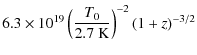
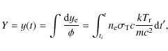
To use the D03PCF routine,
we have to put the Kompaneets equation in the form
where Y is the time variable and X the spatial variable. Here i=1 and
The variables that enter in this equation
are introduced and used in
logarithmic form
to have a good and essentially uniform accuracy of the solution
in the whole frequency range under consideration.
They are ![]() and
and
![]() .
Hereafter, we use the variables X, U, Y for
what concerns the informatic aspect of the problem,
keeping the use of the variables
.
Hereafter, we use the variables X, U, Y for
what concerns the informatic aspect of the problem,
keeping the use of the variables
![]() for considerations directly linked to physical aspects.
The function Ri is determined only
by the inverse Compton term, while the other physical processes,
i.e. at least Compton scattering, bremsstrahlung,
and radiative Compton, are included in the function Qi.
To reduce Eq. (7) into a system
of ordinary differential equations, the D03PCF routine uses the method
of lines: the right member
of Eq. (7) is discretized, reducing the calculation of partial
derivatives in terms of finite values of the
solution vector U on all the points of the X axis grid. Spatial
discretization is made by the method of finite
differences (Mitchell & Griffiths 1980).
The resulting system of ordinary
differential equations is solved using a
differentiation formula method.
The choice of the time parameter was driven by the need to
have a very simple form of the Kompaneets equation. Finally,
a ``temperature independent'' (time) Comptonization parameter
for considerations directly linked to physical aspects.
The function Ri is determined only
by the inverse Compton term, while the other physical processes,
i.e. at least Compton scattering, bremsstrahlung,
and radiative Compton, are included in the function Qi.
To reduce Eq. (7) into a system
of ordinary differential equations, the D03PCF routine uses the method
of lines: the right member
of Eq. (7) is discretized, reducing the calculation of partial
derivatives in terms of finite values of the
solution vector U on all the points of the X axis grid. Spatial
discretization is made by the method of finite
differences (Mitchell & Griffiths 1980).
The resulting system of ordinary
differential equations is solved using a
differentiation formula method.
The choice of the time parameter was driven by the need to
have a very simple form of the Kompaneets equation. Finally,
a ``temperature independent'' (time) Comptonization parameter
has been found to be particularly advantageous (Burigana et al. 1991a).
2.1 Boundary conditions
Integrating equations of the type of Eq. (7) means to calculate the time evolution of the function U(X,Y), for a given initial condition U(X,0). In fact, the problem is also called ``problem at initial conditions''. Numerically, the derivatives of U are replaced by finite differences between values of U computed on a grid of points (in X) and the differential equation is replaced by a system of more simple equations. However, in the presence of the only initial condition, this system is singular (Press et al. 1992). For this reason, resolving partial differential parabolic equations needs boundary conditions. In general, boundary conditions mean additional relations written to be joined to the system derived from the discretization to finite differences.
Therefore, a good statement of the problem needs the definition of
appropriate boundary conditions.
The capability of a refresh of these conditions along the
integration in time leads more stability to the solution evolution
because of the evolution of the radiation field.
Thanks to the opportunity of having the correct value of ![]() for
each time step, the update of the boundary conditions
can be physically motivated (see also Sect. 3.2.6).
The limits of the frequency range considered are
for
each time step, the update of the boundary conditions
can be physically motivated (see also Sect. 3.2.6).
The limits of the frequency range considered are
![]() and
and
![]() .
Of course, we want a solution of the
Kompaneets equation over all the frequency
range where it is possible to measure the CMB.
Also, we need to consider a frequency range wide enough to contain,
in practice, all the energy density of the cosmic radiation field.
The frequency range is so wide for the other two reasons described below.
.
Of course, we want a solution of the
Kompaneets equation over all the frequency
range where it is possible to measure the CMB.
Also, we need to consider a frequency range wide enough to contain,
in practice, all the energy density of the cosmic radiation field.
The frequency range is so wide for the other two reasons described below.
During the time evolution,
some spurious oscillations of the solution
may appear at points close to the boundaries.
These effects
may be partially amplified if, for the computational reasons discussed
in the following, the necessary refreshing of the electronic
temperature is not made for every time step
(but they
could also occur independently of the need to refresh ![]() - for
example for cases at constant
- for
example for cases at constant ![]() ).
Fixing the frequency integration range limits far from the interval
where we are interested
in computing the photon distribution function
allows prevention of
the ``contamination'' of these solution
by possible spurious oscillations in the frequency range
of interest.
).
Fixing the frequency integration range limits far from the interval
where we are interested
in computing the photon distribution function
allows prevention of
the ``contamination'' of these solution
by possible spurious oscillations in the frequency range
of interest.
We can generally assume
that a Planckian spectrum at
![]() is formed
before recombination on a shorter timescale than the
expansion time and, in contrast, at
is formed
before recombination on a shorter timescale than the
expansion time and, in contrast, at
![]() the shape of the spectrum is unknown.
Thus, we implemented in the code
the possibility of adopting
a particular case of Neumann boundary conditions,
i.e. the requirement that the current density, in the frequency space,
is null at the boundaries of the integration range (Chang & Cooper 1970):
the shape of the spectrum is unknown.
Thus, we implemented in the code
the possibility of adopting
a particular case of Neumann boundary conditions,
i.e. the requirement that the current density, in the frequency space,
is null at the boundaries of the integration range (Chang & Cooper 1970):
![\begin{displaymath}\Bigg[\phi\frac{\partial\eta}{\partial x} + \eta(1+
\eta)\Bigg]_{x=x_{\rm min},x_{\rm max}} = 0 .
\end{displaymath}](/articles/aa/full_html/2009/45/aa12061-09/img68.png)
This choice of boundary conditions formally satisfies the requirement of the problem when we integrate the Kompaneets equation in the case of Bose-Einstein-like distortions (with a frequency dependent chemical potential,
Of course, it is possible to make a different choice of the boundary
conditions by selecting Dirichlet-like conditions.
In this case the photon occupation number
at the boundaries of the integration interval does not change
for the whole integration time.
(In general cases, keeping constant conditions at the boundaries
could be dangerous for the continuity of the solution. Nevertheless,
this condition can work
for some specific problems
- typically for problems with constant ![]() ).
).
3 A detailed view on KYPRIX
The code KYPRIX was written to solve the Kompaneets equation in
many kinds of situations.
The physical processes that can be
considered in KYPRIX are: Compton scattering, bremsstrahlung, radiative
Compton scattering, sources of photons, energy injections without photon
production, energy exchanges (heating or cooling processes) associated to
![]() at low redshifts, radiative decays of massive particles,
and so on (see e.g. Danese & Burigana 1994 for some applications).
This code could be easily implemented
to consider other kinds of physical processes.
Various kinds of initial conditions for the problem can be considered,
and many of them have already been implemented in
KYPRIX. The first obvious case is a pure Planckian spectrum.
Several ways to model an instantaneuos heating implying
deviations from the Planckian spectrum have been introduced:
a pure Bose-Einstein (BE) spectrum or a BE spectrum modified to
become Planckian at low frequencies
(this option could be exploited to integrate the
Kompaneets equation with a constant
at low redshifts, radiative decays of massive particles,
and so on (see e.g. Danese & Burigana 1994 for some applications).
This code could be easily implemented
to consider other kinds of physical processes.
Various kinds of initial conditions for the problem can be considered,
and many of them have already been implemented in
KYPRIX. The first obvious case is a pure Planckian spectrum.
Several ways to model an instantaneuos heating implying
deviations from the Planckian spectrum have been introduced:
a pure Bose-Einstein (BE) spectrum or a BE spectrum modified to
become Planckian at low frequencies
(this option could be exploited to integrate the
Kompaneets equation with a constant ![]() and constant boundary conditions);
a grey-body spectrum; a superposition of blackbodies.
and constant boundary conditions);
a grey-body spectrum; a superposition of blackbodies.
The data are saved in five files:
- DATI.
- This file contains the information about the specific parameters of the problem with a general description of its main aspects.
- DATIP.
- In this file we give the evolution of interesting quantities,
such time, redshift,
 ,
and other quantities inherent to the physical and numerical aspects of
the problem (see also Sect. 5.1).
,
and other quantities inherent to the physical and numerical aspects of
the problem (see also Sect. 5.1).
- DATIG.
- It contains the grid of points for the X axis used by
the main program (remember that we are using a dimensionless
frequency), a Planckian spectrum at temperature T0, and the solution
vector
 (that is to say
 )
at y = 0 (starting time).
)
at y = 0 (starting time).
- DATIDE.
- This is the fundamental output file, which gives the solution of the Kompaneets equations at the desired cosmic epochs.
- DATIT.
- It is similar to the file DATIDE, but it contains the solution in term of brightness temperature (i.e. equivalent thermodynamic temperature; see Eq. (12) in Sect. 3.2.2).
3.1 Main subdivisions
The code is divided into several sections and, from a general point of view, is structured as described here.
- 1.
- the main program, where many actions can be carried out: choice of the physical processes, choice of the cosmological parameters, initial conditions, characteristics of the numerical integration (accuracy, number of points of the grid), time interval of interest, choice of the boundary conditions, chemical abundances, ionization history;
- 2.
- subroutine PDEDEF is the subprogram where the problem is numerically defined. This subroutine is also divided in subsections to allow modifications in a simple and practical way;
- 3.
- subroutine BNDARY. Here the boundary conditions are numerically specified;
- 4.
- Subroutines and auxiliary functions perform specific calculations.
3.2 Technical specifications and code implementation
The first version![]() of KYPRIX worked with the Mark 8 version of the NAG numerical
library and were based on the routine D03PGF. The version of the
NAG numerical library currently distributed is the Mark 21,
so an update of the code KYPRIX is necessary to adapt it to this new
package.
of KYPRIX worked with the Mark 8 version of the NAG numerical
library and were based on the routine D03PGF. The version of the
NAG numerical library currently distributed is the Mark 21,
so an update of the code KYPRIX is necessary to adapt it to this new
package.
When KYPRIX starts running, it asks for all the input data: from the declarations of the output files' names to the integration accuracy and features. In the following sections we give a description of the various aspects of the code (and of its update), trying to give relevant hints about computational aspects of the code.
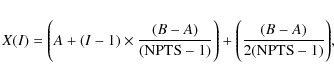
3.2.1 Grid
The frequency integration interval is divided into a grid of points (the mesh points): the larger the number of points, the smaller the adopted frequency step. We adopted an equispaced grid in X. It is possible to use a very dense grid (for example 36 001 mesh points corresponding to 36 000 frequency steps). In general, it is necessary to use at least 3001 mesh points to have an accurate enough solution.
We find a big difference between the two NAG versions, not reported in the documentation of the routine D03PCF. In the first version (D03PGF), the subroutine where the partial differential equation is defined adopted the same mesh points defined in the main program. In the Mark 21 version the calculation is carried out in a different manner: the mesh points used in the subroutine PDEDEF is shifted of half spatial step with respect to the mesh defined in the main program. In this way, the mesh points in the PDEDEF subroutine will be exactly in the middle of the steps defined in the grid of the main program. For this reason, the limits of the integration interval are not considered in the mesh points in the subroutine PDEDEF, and they are used only for the boundary conditions.
The effect of this feature implies the definition of new
parameters that play a fundamental role in
the subroutine PDEDEF.
The integral quantities in the Kompaneets equation
(necessary to define the radiative Compton
term in the kinetic equations and the electron temperature) are computed
once for any time step, inside the PDEDEF subroutine.
For this computation,
arrays of dimension equal to the number of mesh points
of the x variable as defined in the PDEDEF subroutine
are used.
Therefore, a particular care must be taken in the definition
of the dimension of the
arrays defined in KYPRIX.
Those used
in the main program have dimensions equal to the number of points of
the mesh defined in the main program. The same
dimension is given for the arrays defined for the boundary conditions.
On the other hand, the major number of arrays
are used in the PDEDEF subroutine to compute the integral
quantities. The
``inner'' grid adopted in the PDEDEF subroutine is based on mesh points in
the middle of the spatial
steps of the main program grid, so the two grids can not
work with the same point number; in fact, the arrays used in the
PDEDEF subroutine have dimension
![]() .
Therefore, in the main program and in the subroutine BNDARY we have
to work with arrays based on the formula:
.
Therefore, in the main program and in the subroutine BNDARY we have
to work with arrays based on the formula:
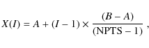
to define the correspondence between the grid of
For continuity reasons, we need to define (according to the choices made in the main program) the solution vector, containing the photon initial distribution function, at the beginning of the integration also according to this grid definition. This vector is used by the PDEDEF subroutine as the initial spectrum adopted for the computation of the rates of the physical processes, and, of course, it is then renewed at every time step incrementation.
3.2.2 Output
Concerning the output files, the updated version of KYPRIX stores a new vector containing the ``inner'' X grid used by the PDEDEF subroutine, XXGR (XGR refers to the main program X grid).
In addition, we preferred to have the
possibility of performing the conversion of the solution
into equivalent thermodynamic temperatures directly
into the code and save it in a new output file (DATIT).
The conversion relation is
(we remember that in the code
The fundamental reason for performing this conversion directly in the code is associated to the extreme accuracy required for the solution in the case of very small distortions, of particular interest given the FIRAS results (Fixsen et al. 1996). During the first tests, the conversion of the solution in brightness temperature was performed at the same time as the solution visualization, through the IDL visualization program. Saving the solution into files is typically performed, not for all the points of the grid, but for a reduced grid of, for example, 300 equidistant points along the original grid to avoid to store files of large size, useless for our scope, given the interest for the CMB continuous spectrum (by definition, the Kompaneets equation is not appropriate to treating recombination lines). If the considered distortions were very small, then the solution at each specific ``inner'' grid point could be affected by a numerical uncertainty that is not negligible in comparison with the very small deviations from a Planckian spectrum relevant in these cases. This numerical error is greatly reduced (becoming negligible for our purposes) by the averaging over a suitable number of grid points. Of course, the storing of the solution directly on a limited number of grid points makes this averaging no longer possible on the stored data. It is then necessary to average the solution values in intervals corresponding to the output x grid directly into the code. In many circumstances, the diagram shape derived by applying the conversion to brightness temperature only on the stored averaged solution still deviates at high frequencies from the effectively computed solution displayed by considering all the ``inner'' grid points because of the high gradients in the photon distribution function and/or in the brightness temperature that makes it difficult, or impossible, to find a general rule for the solution binning that simultaneously works properly for the two solution representations. This problem is avoided by converting the solution vector in equivalent thermodynamic temperature before the binning of its values and then applying the binning to the equivalent thermodynamic temperature. The result is then a very clean and precise brightness temperature diagram, even for very small distortions.
Other minor changes we made in the output data, where we pass from real to double precision, and in the frequency of storing results into the output files.
3.2.3 Equation formalism
A necessary update of the code was performed to adapt it
to the different formalism adopted by the new version of the NAG routine.
This regards the expression of the Kompaneets equation in the PDEDEF
subroutine.
In particular, the D03PGF routine adopted the following expression
of the partial differential equation:
![\begin{displaymath}C_i \frac{\partial U_i}{\partial Y} =
X^{-m} \sum_{j=1}^{\rm...
...gg[ X^m G_{ij}
\frac{\partial U_j}{\partial X} \Bigg] + F_i ,
\end{displaymath}](/articles/aa/full_html/2009/45/aa12061-09/img82.png)
where
It is simple to translate the code from the old to the new formalism.
In the case
![]() .
In this case, we have simply that
R1 contains both the function G1 and
the vector solution derivative with respect to X according to
.
In this case, we have simply that
R1 contains both the function G1 and
the vector solution derivative with respect to X according to
At this point, it is necessary to apply only the following substitutions:
With respect to this formalism, it is not difficult to adapt the various terms of the Kompaneets equation to the D03PCF routine. The terms that describe radiative Compton, bremsstrahlung, (optional) electromagnetic processes, and part of the contribution of the Compton scattering are counted in the function Q1. Instead, the second derivative of the solution vector with respect to X, which represents part of the inverse Compton rate, is counted in the function R1, so, according to these settings, we can write:
where
| |
= | 
|
|
![$\displaystyle + 2 \times 10^X 10^U \left(\frac{\partial U}{\partial X}
+ 2 \right)\bigg] \frac{1}{{\rm ln}(10)}$](/articles/aa/full_html/2009/45/aa12061-09/img95.png)
|
(17) |
and
![$\displaystyle {\rm FBREM+FRAD} = \frac{\left({{\rm e}^{10^X}}\right)^\phi}{10^{...
...c{1}{10^U}-\left[{\left({\rm e}^{10^X}\right)}^{{\phi}^{-1}} - 1\right]\right\}$](/articles/aa/full_html/2009/45/aa12061-09/img96.png)
|
|||
|
(18) |
where
The inverse Compton contributes to R1 in this way:
|
(19) |
Finally, we can put P11 = 1.
Furthermore, it is possible to add other source
terms![]() in Eq. (16).
in Eq. (16).
3.2.4 Boundary conditions
Also notable are the differences between the input
expressions defining the boundary conditions.
The D03PGF routine
adopted an expression of the form
where
where
| (22) |
where XVA is the vector related to the X position computed in A, and the dimension of both the equations corresponds to the differential equation number. Similar conditions are defined for the other extreme of the integration interval [A, B].
3.2.5 Accuracy parameters
Another considerable difference between the two library versions regards the definition of the integration accuracy parameter. D03PGF used three parameters for monitoring the local error estimate in the time direction, supplying a good versatility. RELERR and ABSERR were respectively the quantity for the relative and absolute components to be used in the error test. The third parameter, INORM, was used to define the error test. If E(i,j) is the estimated error for Ui (the vector solution) at the jth point of the X grid, then the error test was
- INORM

- INORM

- INORM
 .
.
This is equivalent to the error test implemented in the D03PGF routine in the case INORM = 0 and ABSERR = RELERR (= ACC).
3.2.6 Electron temperature
During the numerical integration,
some subprograms use the
distribution function calculated at that time to compute ![]() .
The integrals to be computed are those that we
find in the expression for
.
The integrals to be computed are those that we
find in the expression for
![]() :
:
In this calculation, the integration range is obviously the integration interval considered for the problem:
In the previous version of the code KYPRIX,
integral quantities were computed
through a specific modification of the
NAG package implemented by the KYPRIX code author that allowed
recovery of the whole vector solution at each time step
in the subroutines (and in particular in PDEDEF), while the
original package made the solution only available in PDEDEF
separately at each grid point (the package
originally designed for ``pure'' partial differential equation,
without terms involving integrals of the solution). This modification,
possible thanks to the availability of the NAG sources (and, in practice,
thanks to the relative simplicity of the early library versions),
permitted updating the integral quantities perfectly according
to the ``implicit'' scheme adopted by the code for the integration in
time.
This is no longer feasible. Therefore, the update of the integral
quantities must now be performed with a ``backward'' scheme, saving
the solution at the previous time step in a proper vector
and using it in the computation at the given time step.
As is well known, ``backward'' schemes are typically less stable
than implicit schemes.
And, in fact, we verified in some cases
the difficulty of the
D03PCF routine to work implementing the update of the quantities
corresponding to the integral
terms in the Kompaneets equation (and in particular of ![]() )
for each time step.
This was likely caused by numerical instabilities.
)
for each time step.
This was likely caused by numerical instabilities.
We then introduced a new integer control parameter into the code:
STEPFI.
It determines the frequency for the update of the dimensionless electron
temperature ![]() ,
relevant, of course, in case we want to perform an integration with a
variable
,
relevant, of course, in case we want to perform an integration with a
variable ![]() .
We have checked that updating the integral
terms in the Kompaneets equation not at every time step, but after
a suitable number of time steps does not affect the accuracy of the
solution. This is because the time increasing in the code
is performed with very small steps, while the physical variation
of
.
We have checked that updating the integral
terms in the Kompaneets equation not at every time step, but after
a suitable number of time steps does not affect the accuracy of the
solution. This is because the time increasing in the code
is performed with very small steps, while the physical variation
of ![]() occurs on longer timescales
occurs on longer timescales![]() .
See Sect. 5.2.2 for tests regarding the
implications of this new implementation of the electron temperature
evolution.
.
See Sect. 5.2.2 for tests regarding the
implications of this new implementation of the electron temperature
evolution.
3.2.7 Radiative Compton
In computing of the radiative Compton term there is an integral term,
I1, given by the numerator of the right member of Eq. (25)
(see Eq. (16) in Burigana et al. 1995),
so it is necessary to harmonize its update
according to the parameter STEPFI discussed in the previous subsection.
In fact,
a possible asynchronous update of it and
![]() could create numerical instabilities
and the crash of the code run, as physically evident from the
strong relevance of both radiative Compton term
(at least at high redshifts)
and electron
temperature for the evolution of the low-frequency region of the
spectrum.
could create numerical instabilities
and the crash of the code run, as physically evident from the
strong relevance of both radiative Compton term
(at least at high redshifts)
and electron
temperature for the evolution of the low-frequency region of the
spectrum.
3.2.8 Integration routines
The global accuracy of the code KYPRIX depends on the accuracy
of the solver for the partial differential equation, as well as on the
accuracy of all the other routines dedicated to different specific
computations.
In this section we focus on the routines of numerical integration
used in the KYPRIX.
As discussed in the previous sections, the D01GAF routine has been
used for tabulated functions. On the other hand,
KYPRIX involves computing the integrals
of various functions defined by analytical expressions, namely
the parameters characterizing different types of initial conditions for
the distorted spectra, such as the amount of fractional injected
energy, the electron temperature, and the relationship between the
different time variables entering into the code (see also
Sect. 4.1).
Ultimately, the better accuracy in these specific computations
implies a better global accuray for KYPRIX.
In the early release of the code KYPRIX,
the NAG D01BDF routine was used to calculate
integrals of a function over a finite interval.
The same task can be carried out by the D01AJF routine.
This code offers a better
accuracy than D01BDF (D01AJF is in fact suitable also
to integrating functions with singularities,
both algebraic and logarithmic). After the routines
substitution, the results show a strong increase in accuracy.
In particular, this improvement offers the possibility of
also investigating very small distortions that require a very precise
determination
of all the relevant quantities because the absolute numerical error
of the integration must be much smaller than the (very small
quantities) of interest in these cases.
In particular, the quantity
![]() (where
(where
![]() is the actual
density energy and
is the actual
density energy and
![]() the energy density corresponding to the unperturbed distribution function
just before the energy injection)
must be constant during all the
integration process in the absence of energy injection terms,
according to the energy conservation.
The increase in precision on the computation of this quantity
was noteworthy, now always keeping inside a few percent of the
physical value (and its possible physical variation; see
Sect. 5.1)
of the same quantity independently of the magnitude of the
considered distortion, at the same time allowing an accurate
check of the global accuracy of the code, improved thanks
to better computation of all the
integral terms appearing in the Kompaneets equation.
The remarkable improvement in energy conservation,
even in the case of very small distortions,
is an important feature of the new version of KYPRIX
that makes is applicable to a wider set of cases.
the energy density corresponding to the unperturbed distribution function
just before the energy injection)
must be constant during all the
integration process in the absence of energy injection terms,
according to the energy conservation.
The increase in precision on the computation of this quantity
was noteworthy, now always keeping inside a few percent of the
physical value (and its possible physical variation; see
Sect. 5.1)
of the same quantity independently of the magnitude of the
considered distortion, at the same time allowing an accurate
check of the global accuracy of the code, improved thanks
to better computation of all the
integral terms appearing in the Kompaneets equation.
The remarkable improvement in energy conservation,
even in the case of very small distortions,
is an important feature of the new version of KYPRIX
that makes is applicable to a wider set of cases.
4 New physical options
4.1 Cosmological constant
About ten years ago, the relevance of the cosmological constant term (or
of dark energy contribution) was probed by a wide set of
astronomical observations of type Ia supernovae (Riess et al. 1998; Perlmutter et al. 1999).
We then updated the numerical integration code KYPRIX
to include the cosmological constant in the terms controlling the
general expansion of the Universe.
In particular the input background cosmological
parameters considered in the code are now
![]()
![]() ,
i.e. the present CMB temperature, the contribution of massless
neutrinos, the Hubble constant, the (non relativistic) matter
and baryon energy density, the energy densities corresponding
to cosmological constant and curvature terms.
,
i.e. the present CMB temperature, the contribution of massless
neutrinos, the Hubble constant, the (non relativistic) matter
and baryon energy density, the energy densities corresponding
to cosmological constant and curvature terms.
To compute the proper cosmic evolution of the various terms,
a scale factor parameter ![]() (increasing with time)
(Silk & Stebbins 1983),
defined by
(increasing with time)
(Silk & Stebbins 1983),
defined by
has been adopted (here
which is the initial ratio between matter energy density and radiation energy density, and
![\begin{displaymath}\frac{1}{\tau_{g1}} = \bigg(\frac{8\pi}{3} G \rho_{r1}\bigg)^...
...{m_{\rm e}c^2}{k}\bigg)^4\bigg]^{1/2}
= 0.076~\textrm{s}^{-1}
\end{displaymath}](/articles/aa/full_html/2009/45/aa12061-09/img129.png)
defined as a initial gravitational time scale. The quantities with the index 1 refer to the epoch when a = a1, with the index 0 when t = t0 (today);
respectively.
Now we can define an equation for the evolution of ![]() :
:
![$\displaystyle \bigg[\frac{8\pi}{3} G \rho(\omega)\bigg]^{1/2}$](/articles/aa/full_html/2009/45/aa12061-09/img136.png)
![$\displaystyle \frac{8\pi}{3}G\bigg[\frac{\rho_{r1}\kappa}{\omega^4} +
\frac{\rho_{m1}}{\omega^3} +
\frac{\rho_{K1}}{\omega^2} + \rho_{\Lambda}\bigg],$](/articles/aa/full_html/2009/45/aa12061-09/img137.png)
where we have included the contribution of massless relativistic neutrinos in the term
![\begin{displaymath}\frac{1}{\dot{\omega}} = \frac{\tau_{g1}\;\omega}{\bigg[1 + \...
...ambda/m}\;\omega^3}{2.164 \times
10^{27}}\bigg)\bigg]^{1/2}},
\end{displaymath}](/articles/aa/full_html/2009/45/aa12061-09/img139.png)
where
The equation for
![]() has to be inserted in the expression
giving
has to be inserted in the expression
giving
![]() ,
which is inside the integral used to compute the time variable
,
which is inside the integral used to compute the time variable
![]() because we set
y=0 when the integration starts at
because we set
y=0 when the integration starts at
![]() (or equivalently at
(or equivalently at
![]() ).
Finally, the
expression for the time evolution of
).
Finally, the
expression for the time evolution of ![]() and y
are related by the variable change:
and y
are related by the variable change:
where
Implementation of the cosmological constant and curvature
terms makes the code KYPRIX suitable to being applied to interesting
cases at late ages, including cosmic epochs at
z < 1 when ![]() supplies the greatest contribution to the expansion
rate of the Universe.
Remarkable examples are spectral distortions
associated to the re-ionization of the Universe, which
starts at relatively low redshifts (
supplies the greatest contribution to the expansion
rate of the Universe.
Remarkable examples are spectral distortions
associated to the re-ionization of the Universe, which
starts at relatively low redshifts (
![]() )
in typical astrophysical scenarios.
For the sake of completeness,
a few words are needed about the computation of the time
evolution in the code. The subroutine called WDIY0 is the core of the
time evolution in KYPRIX: it computes the value of
)
in typical astrophysical scenarios.
For the sake of completeness,
a few words are needed about the computation of the time
evolution in the code. The subroutine called WDIY0 is the core of the
time evolution in KYPRIX: it computes the value of ![]() given a value
of y. This process takes advantage of the definition of y as
the integral of
dy and, of course, it happens at each time step. To do this, we make use
of a double precision version of the function ZBRENT, from
``Numerical Recipes'' (Press et al. 1992).
given a value
of y. This process takes advantage of the definition of y as
the integral of
dy and, of course, it happens at each time step. To do this, we make use
of a double precision version of the function ZBRENT, from
``Numerical Recipes'' (Press et al. 1992).
4.2 Chemical abundances
In this new version of the code, it is possible to choose the primordial
abundances of H and He. We have consistently computed
the electron number density,
![]() ,
involved in the different physical processes.
In the previous implementation, it was assumed a fixed abundance of H
and He (and full ionization).
The electron number density was then given by
,
involved in the different physical processes.
In the previous implementation, it was assumed a fixed abundance of H
and He (and full ionization).
The electron number density was then given by
|
(33) |
where
|
(34) |
This obviously affects the physical processes involved in the code. Compton scattering, radiative Compton, and bremsstrahlung depend linearly
4.3 Ionization history
In the past years, CMB observations are achieving a very high
accuracy, in particular regarding the angular power spectrum
of temperature anisotropies, but also for that of
E mode polarization and cross-correlation (see e.g. Nolta et al. 2009).
A detailed understanding of the cosmological reionization process
is crucial for precisely modeling the power spectrum of CMB
anisotropies in comparison with current data, while a better
treatment of recombination is very relevant in view
of the data expected by the forthcoming ESA Planck
satellite![]() (The Planck Collaboration 2006).
(The Planck Collaboration 2006).
Accurate modeling of the ionization history is also crucial for precisely computing of CMB spectral distortions in view of the comparison with data from a future generation of high-sensitivity experiments. We then included these aspects in the current implementation of KYPRIX. In particular, the fraction of each state of ionization of the relevant elements (H and He) has been implemented.
The effects of this implementation is negligible![]() in practice for the
radiative Compton, because this process is important at high redshifts
when the medium is fully ionized.
Instead, Compton scattering and bremsstrahlung rates are significantly
influenced by this implementation.
Once introduced, the electron ionization fraction in the code,
in practice for the
radiative Compton, because this process is important at high redshifts
when the medium is fully ionized.
Instead, Compton scattering and bremsstrahlung rates are significantly
influenced by this implementation.
Once introduced, the electron ionization fraction in the code,
![]() ,
which gives the number of electrons that takes
part in the physical processes, we can choose different ways
the active fractions of elements can play their roles in the phenomena.
,
which gives the number of electrons that takes
part in the physical processes, we can choose different ways
the active fractions of elements can play their roles in the phenomena.
Given
![]() ,
from the charge conservation law, we have a constraint
on the number of the free ions in the considered plasma.
The simplest way to account for them in
the code is to assume an equal fraction of ionization for H and He.
Of course, this is a toy model, but this parametrization was
very useful for testing the code.
,
from the charge conservation law, we have a constraint
on the number of the free ions in the considered plasma.
The simplest way to account for them in
the code is to assume an equal fraction of ionization for H and He.
Of course, this is a toy model, but this parametrization was
very useful for testing the code.
A somewhat more accurate treatment of the physics of
reionization/recombination processes
implemented in the code is based on the Saha equation:
|
(35) |
where ni is the density of atoms in the ith state of ionization,
|
(36) |
Providing the electron ionization fraction defined as

|
(37) |
we can compute the unknowns
To recover all the unknowns we need other relations. These additional conditions are provided by the charge conservation and the nuclei conservation. From charge conservation it is possible to recover the contribution of the electrons related to a single specie to the total number of free electrons. The latter is of course related to the ionization fraction of all the involved species and can be written as:
![\begin{displaymath}n_{\rm e}^{\rm free} = \frac{\rho_{\rm b}}{m_{\rm b}} \left[ ...
...eft(\chi_{{\rm He}^+} + \chi_{{\rm He}^{++}} \right) \right] ,
\end{displaymath}](/articles/aa/full_html/2009/45/aa12061-09/img166.png)
where
The nuclei conservation law separately for H and He
is expressed by
![\begin{displaymath}n_{\rm H}^{\rm tot} = \frac{\rho_{\rm b}}{m_{\rm b}} \left[ f_{\rm H} \left(\chi_{\rm H} + \chi_{\rm H^+}\right) \right] ,
\end{displaymath}](/articles/aa/full_html/2009/45/aa12061-09/img167.png)
|
(40) |
![\begin{displaymath}n_{\rm He}^{\rm tot} = \frac{\rho_{\rm b}}{m_{\rm b}} \left[\...
...{\rm He} +
\chi_{{\rm He}^+} + \chi_{{\rm He}^{++}}) \right].
\end{displaymath}](/articles/aa/full_html/2009/45/aa12061-09/img168.png)
|
(41) |
Providing the electron ionization fraction and the temperature, it is possible to build two separate systems (one for H and one for He) in order to recover the considered ionization fractions. The code can ingest a table with the desired evolution of
The best way to perform the exact
calculation of the rates of considered processes in scenarios involving
reionization/recombination
uses a co-running code, coupled to KYPRIX, able to supply the
ionization fraction for all the species.
For the recombination process,
we developed an interface that allows the code to call an external program,
in our case RECFAST (Seager et al. 1999), and run it with the same
cosmological parameters selected for KYPRIX.
Then KYPRIX will read the output table from RECFAST and use
the ionization fractions for
the calculation of the rates of the processes, allowing a more detailed
estimation of the spectral distortion arising during the
recombination process (Wong et al. 2008). If we are interested in
standard recombination, we adopt the equilibrium electron
temperature (Eq. (25)).
A consistent modeling of a modified recombination should provide
the evolution of both electron temperature and ionization fractions
(at least
![]() ).
).
5 Tests on code performance, reliability, and accuracy
Once terminated the updating of the numeric integration code, we carried out many accuracy and performance tests. Obviously, we checked the physical meaning of the numerical solutions provided by the code comparing them with the existing analytical solutions that in some cases can be considered as good approximations of exact solutions. In general, a code of good quality must have high numerical precision compared to the knowledge, both theoretical and observational, of the problem. Various routines, mainly from the NAG package, but also from the ``Numerical Recipes'' (Press et al. 1992) package, we used for several specific computations. Since different routines can solve the same mathematical problems using different numerical methods and/or implementations with different settings and input parameters, we verified that the adopted routines allow the appropriate accuracy and efficiency. In the following we report on some specific quality tests of the numerical solutions. We comment now briefly on the code computational time.
To evaluate the global CPU time of the code,
we performed many runs with very different settings.
These times we carried out testing the code on a
machine with 4 Alpha CPUs, but effectively using only one CPU
(now we are running the code on IBM Power5 Processors).
The code's global CPU time ranges from a few minutes,
for cases in which the integration
starts at low redshifts, to about 5 h for some cases starting at
very high redshifts (
![]() ).
There are many
variables that play a role in determining the global CPU time.
The complete Kompaneets equation in fact involves several terms.
In the code KYPRIX we can select the physical processes
to be considered in the numerical integration, and the global CPU time
increases with the number of activated processes.
).
There are many
variables that play a role in determining the global CPU time.
The complete Kompaneets equation in fact involves several terms.
In the code KYPRIX we can select the physical processes
to be considered in the numerical integration, and the global CPU time
increases with the number of activated processes.
Of course, the global CPU time depends on the
parameters related to the numerical integration characteristics.
The number of points adopted for the X grid
(see Sect. 3.2.1)
has a strong influence on
the global CPU time.
Clearly, the integration accuracy improves with NPTS,
and in many cases it must be set to a very high value.
We find that the global CPU time
is approximately proportional to NPTS (
![]() ).
).
The parameter that plays the most relevant role
in determining the global CPU time
is the accuracy required for the time integration.
The final solution precision depends on the value of the corresponding
parameter ACC.
Only for very high accuracy
(ACC
![]() )
does the CPU
time reach the duration of some hours while keeping
ACC
)
does the CPU
time reach the duration of some hours while keeping
ACC
![]() the integration is carried out in a few minutes.
The limits imposed by CMB spectrum observations drive us to investigate
the small distortions in particular.
It is then necessary to work with low values of ACC (in general,
the integration is carried out in a few minutes.
The limits imposed by CMB spectrum observations drive us to investigate
the small distortions in particular.
It is then necessary to work with low values of ACC (in general,
![]() 10-8).
10-8).
After assessing of the better choice for using of the parameters of the various numerical routines and the definition of the accuracy of the integration in time, we carried out several tests to verify the physical validity of the code results.
5.1 Energy conservation
In the code output file DATIP, we stored values of several parameters of
interest.
Two of them provided very useful information on the
goodness of the numerical integration.
The first one is the ratio,
![]() ,
between the radiation energy density at each time and the energy density
corresponding to the unperturbed distribution function before
the distortion
,
between the radiation energy density at each time and the energy density
corresponding to the unperturbed distribution function before
the distortion![]() in the absence of dissipation processes. The exact energy conservation
is represented by the constance of this ratio during the integration.
To quantify the accuracy supplied by KYPRIX,
the values of
in the absence of dissipation processes. The exact energy conservation
is represented by the constance of this ratio during the integration.
To quantify the accuracy supplied by KYPRIX,
the values of
![]() we stored
at the start of the integration and at many times thereafter.
In order to estimate the precision of the energy conservation,
we define the quantity:
we stored
at the start of the integration and at many times thereafter.
In order to estimate the precision of the energy conservation,
we define the quantity:
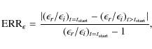
which gives the relative induced error in the energy conservation with respect to the initial value of
![\begin{figure}
\par\includegraphics[width=8.5cm,clip]{nrg.ps}
\end{figure}](/articles/aa/full_html/2009/45/aa12061-09/img182.png)
|
Figure 1:
Error in the energy conservation expressed in terms of
relative (%) deviation from its input value of the quantity
|
| Open with DEXTER | |
Since the same absolute numerical integration error
corresponds to a larger relative error for a smaller distortion,
i.e. for smaller
![]() in these models,
we could in principle expect a relative degradation of the energy
conservation for decreasing distortion amplitudes.
Our tests in fact indicate an increase
in the relative degradation of the energy conservation
for decreasing distortions when the same accuracy parameters are
adopted.
On the other hand, one can select them according the specific problem.
For example, considering an energy injection of
in these models,
we could in principle expect a relative degradation of the energy
conservation for decreasing distortion amplitudes.
Our tests in fact indicate an increase
in the relative degradation of the energy conservation
for decreasing distortions when the same accuracy parameters are
adopted.
On the other hand, one can select them according the specific problem.
For example, considering an energy injection of
![]() occurred at
occurred at
![]() ,
an accuracy equal to
,
an accuracy equal to
![]() is fully satisfactory
for a very precise calculation of the
photon distribution function;
while for earlier processes, such as for
is fully satisfactory
for a very precise calculation of the
photon distribution function;
while for earlier processes, such as for
![]() ,
and for the same injected fractional energy,
the accuracy parameter needs to be set to
,
and for the same injected fractional energy,
the accuracy parameter needs to be set to
![]() to assure a
calculation with
to assure a
calculation with
![]() less than 1%.
We find that for suitable choices of the integration accuracy
parameters,
less than 1%.
We find that for suitable choices of the integration accuracy
parameters,
![]() can always be kept
below
can always be kept
below ![]()
![]() without requiring too a long computational time.
Finally, we note that in some circumstances
the scheme for the electron temperature evolution
in the new version of KYPRIX (backward differences),
different from that used in the original one (implicit scheme),
could imply some small discontinuities in the evolution
of the electron temperature
and of
without requiring too a long computational time.
Finally, we note that in some circumstances
the scheme for the electron temperature evolution
in the new version of KYPRIX (backward differences),
different from that used in the original one (implicit scheme),
could imply some small discontinuities in the evolution
of the electron temperature
and of
![]() .
On the other hand,
we have verified that this does not affect the
accuracy of the solution, because of the very small amplitude of these
discontinuities (together with their localization to a very limited
number of time steps) and of the corresponding energy
conservation violation.
.
On the other hand,
we have verified that this does not affect the
accuracy of the solution, because of the very small amplitude of these
discontinuities (together with their localization to a very limited
number of time steps) and of the corresponding energy
conservation violation.
5.2 Comparative tests
5.2.1 Comparing solutions
The first kind of test is a simple comparison between the results obtained with the updated version of KYPRIX and those obtained with the original version for the same set of input parameters.
To do this, we have considered some interesting cases
carried out in the past. In particular we used the input parameters
adopted in
(Burigana et al. 1995)
where semi-analytical descriptions
of the numerical solutions of the Kompaneets equation were also
reported.
We report here cases characterized by
a specific amount of exchanged fractional energy
![]() .
We started the
integration from a redshift
corresponding to
.
We started the
integration from a redshift
corresponding to
![]() in one case
and to
in one case
and to
![]() in another.
The input cosmological parameters are
in another.
The input cosmological parameters are
![]() K.
The results given by the update
version of KYPRIX
are fully consistent with those reported in
Burigana et al. (1995)
(see Fig. 2 and
note the excellent agreement between the results of the two codes).
Moreover, since that paper also provided a seminalytical
description of the solution of the
Kompaneets equation,
it is clear that the good agreement of the numerical results
obtained with the original and update code represents
further confirmation of the validity of the analytical
description.
K.
The results given by the update
version of KYPRIX
are fully consistent with those reported in
Burigana et al. (1995)
(see Fig. 2 and
note the excellent agreement between the results of the two codes).
Moreover, since that paper also provided a seminalytical
description of the solution of the
Kompaneets equation,
it is clear that the good agreement of the numerical results
obtained with the original and update code represents
further confirmation of the validity of the analytical
description.
![\begin{figure}
\par\includegraphics[angle=270,width=8.2cm,clip]{compa.ps}
\end{figure}](/articles/aa/full_html/2009/45/aa12061-09/img192.png)
|
Figure 2:
Comparison between the present time solution
for the CMB spectrum obtained from the old version of
the numerical code ( top panel;
adapted from panel a of Fig. 1 in Burigana et al. 1995)
and the current one ( bottom panel).
See the text for further details on computation parameters.
Dashed (dot-dashed) line refers to an energy injection occurred at
|
| Open with DEXTER | |
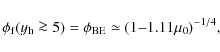
5.2.2 Electron temperature behavior
While the energy exchange between matter and radiation
is led by Compton scattering
(in the absence of external energy dissipation processes),
electrons reach the equilibrium Compton temperature
(Peyraud 1968; Zeldovich & Levich 1970),
![]() ,
in a shorter time than the expansion time. For
,
in a shorter time than the expansion time. For
![]() ,
(late heating processes) Compton scattering is no longer able to
significantly modify
the shape of the perturbed spectrum, and the final electronic
temperature
,
(late heating processes) Compton scattering is no longer able to
significantly modify
the shape of the perturbed spectrum, and the final electronic
temperature
![]() (remember
that
(remember
that
![]() )
immediately after the decoupling is very close
to
)
immediately after the decoupling is very close
to
![]() .
On the other hand, for energy injections at redshifts corresponding
to
.
On the other hand, for energy injections at redshifts corresponding
to
![]() ,
Compton scattering can establish kinetic equilibrium between
matter and radiation. This
corresponds to a Bose-Einstein spectrum,
with a final electron temperature given by
(Danese & de Zotti 1977; Sunyaev & Zeldovich 1970)
,
Compton scattering can establish kinetic equilibrium between
matter and radiation. This
corresponds to a Bose-Einstein spectrum,
with a final electron temperature given by
(Danese & de Zotti 1977; Sunyaev & Zeldovich 1970)
where
For the intermediate energy injection epochs, corresponding to
![]() ,
the final value of
,
the final value of ![]() (a function depending on
(a function depending on ![]() )
is between the values of
)
is between the values of
![]() and
and
![]() ,
because the Compton
scattering works to produce a Bose-Einstein like spectrum
anyway (Burigana et al. 1991a).
At these epochs the relation between the chemical potential and the amount of
fractional injected energy injected is simply given by
(Danese & de Zotti 1977; Sunyaev & Zeldovich 1970):
,
because the Compton
scattering works to produce a Bose-Einstein like spectrum
anyway (Burigana et al. 1991a).
At these epochs the relation between the chemical potential and the amount of
fractional injected energy injected is simply given by
(Danese & de Zotti 1977; Sunyaev & Zeldovich 1970):

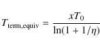
By exploiting the numerical results, a simple formula for
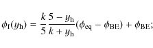
here k=0.146 is a constant derived from the fit. Moreover, this expression represents an accurate description of the evolution of
In these cases, as in many situations of interest, the perturbed spectrum of the radiation (immediately after the heating process) is described by a superposition of blackbodies and the equilibrium temperature is given by (Burigana et al. 1995; Zeldovich & Sunyaev 1969; Zeldovich et al. 1972)
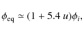
where
Equations (45) and (46) can be used to test the behavior of the electron temperature during the numerical integration of the Kompaneets equation carried out with the new code version. With the increase in the time variable, the values of
![\begin{figure}
\par\includegraphics[width=8.8cm,clip]{FI.ps}
\vspace*{4mm}
\end{figure}](/articles/aa/full_html/2009/45/aa12061-09/img215.png)
|
Figure 3:
Top panel: evolution of |
| Open with DEXTER | |
This test is of particular importance for checking the validity
of the results
because of the crucial role of ![]() in the Kompaneets equation.
As remembered in the previous section,
in the new version of the code a different scheme is
used than implemented in the original version.
Verifying of the very good agreement of these behaviors of
in the Kompaneets equation.
As remembered in the previous section,
in the new version of the code a different scheme is
used than implemented in the original version.
Verifying of the very good agreement of these behaviors of ![]() further supports the equivalence of the two code versions
and their reliability.
In particular, it confirms that
the new adopted numerical scheme for the evolution of
further supports the equivalence of the two code versions
and their reliability.
In particular, it confirms that
the new adopted numerical scheme for the evolution of ![]() ,
in principle less stable than the implicit scheme
implemented in the code original version, does not affect
the validity of the solution.
,
in principle less stable than the implicit scheme
implemented in the code original version, does not affect
the validity of the solution.
5.3 Free-free distortion
As already discussed in Sunyaev & Zeldovich (1970),
accurate measures of the CMB spectrum
in the Rayleigh-Jeans region could provide quantitative informations about the
thermal
history of the Universe at primordial cosmic epochs.
On the other hand, photon production processes (mainly radiative Compton at earlier
epochs and
bremsstrahlung at later epochs) work to reduce the CMB spectrum depression at long
wavelengths (see Danese & de Zotti 1980)
since they try to establish a true (Planckian) equilibrium.
For
![]() (Burigana et al. 1991a; Danese & de Zotti 1980) with
(Burigana et al. 1991a; Danese & de Zotti 1980) with
low-frequency photons are absorbed before Compton scattering moves them to higher frequencies.
In the case of small and late distortions (
![]() ), a
good approximation of the
whole spectrum is given by (Burigana et al. 1995)
), a
good approximation of the
whole spectrum is given by (Burigana et al. 1995)
where the index i denotes the initial value of the corresponding quantity and u is the Comptonization parameter. This expression provides also an exhaustive description of continuum spectral distortion generated in various scenarios of (standard or late) recombination or associated to the cosmological reionization. For an initial blackbody spectrum at dimensionless frequencies
|
(51) |
Here,
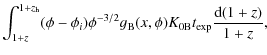
where
In terms of brightness temperature, the distortions at low frequencies
(at any redshift) can be written as
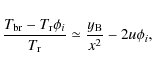
where
To show that our numerical solution follows the behavior
described by the above equation, we can compute
![]() from the brightness temperature derived from the numerical solution:
from the brightness temperature derived from the numerical solution:
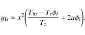
The reported numerical result (see Fig. 4) refers to a heating process corresponding to a full reionization starting at
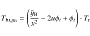
in comparison with the numerical results. Where the Gaunt factor dependence on x and
The use of
![]() in
Eq. (55)
implies a slight excess
(
in
Eq. (55)
implies a slight excess
(![]()
![]() )
with respect to the accurate numerical results
since
)
with respect to the accurate numerical results
since ![]() decreases with the frequency (see Fig. 4).
In this representative test, the excess is
decreases with the frequency (see Fig. 4).
In this representative test, the excess is ![]() 0.1 mK, but
obviously its value depends on the amplitude of free-free distortion
(other than on the frequency).
This error is clearly negligible for analysis of current data (see e.g.
Salvaterra & Burigana 2000; Zannoni et al. 2008; Salvaterra & Burigana 2002; Singal et al. 2009).
It is likely not so relevant for
analyzing future measures at
0.1 mK, but
obviously its value depends on the amplitude of free-free distortion
(other than on the frequency).
This error is clearly negligible for analysis of current data (see e.g.
Salvaterra & Burigana 2000; Zannoni et al. 2008; Salvaterra & Burigana 2002; Singal et al. 2009).
It is likely not so relevant for
analyzing future measures at
![]() cm with
accuracy comparable to what is proposed for DIMES (Kogut 1996; Burigana & Salvaterra 2003).
On the contrary, it could be relevant
for a very accurate analysis of
future measures with precision comparable to what
is proposed for FIRAS II
cm with
accuracy comparable to what is proposed for DIMES (Kogut 1996; Burigana & Salvaterra 2003).
On the contrary, it could be relevant
for a very accurate analysis of
future measures with precision comparable to what
is proposed for FIRAS II
![]() cm (Fixsen & Mather 2002; Mather 2009; Burigana et al. 2004)
or conceived for possible future long wavelength experiments
from the
Moon
cm (Fixsen & Mather 2002; Mather 2009; Burigana et al. 2004)
or conceived for possible future long wavelength experiments
from the
Moon![]() ,
,![]() (Burigana et al. 2007).
This calls for a complete frequency and thermal
history-dependent treatment of the free-free distortion
in the accurate analysis of future data of extreme accuracy.
(Burigana et al. 2007).
This calls for a complete frequency and thermal
history-dependent treatment of the free-free distortion
in the accurate analysis of future data of extreme accuracy.
![\begin{figure}
\par\includegraphics[width=8.5cm,clip]{yb.ps}
\end{figure}](/articles/aa/full_html/2009/45/aa12061-09/img243.png)
|
Figure 4:
Top panel: |
| Open with DEXTER | |
6 Discussion and conclusion
We have described the fundamental numerical approach and, in particular, the recent update to recent NAG versions of a numerical code, KYPRIX, specifically written to solve the Kompaneets equation in a cosmological context, aimed at very accurate computation of the CMB spectral distortions under quite general assumptions. The recipes and tests described in this work can be useful for implementing accurate numerical codes for other scientific purposes using the same or similar numerical libraries or for verifying the validity of different codes aimed at the same or similar problems.
Specifically, we discussed the main subdivisions of the code and the most relevant aspects about technical specifications and code implementation. After presenting the equation formalism and the boundary conditions added to the set of ordinary differential equations derived from the original parabolic partial differential equation, we gave details on the adopted space (i.e. dimensionless frequency) grid, on the output results, on the accuracy parameters, and on the integration routines. The time dependence of the ratio between electron and photon temperatures and of the radiative Compton scattering term, both introducing integral terms into the Kompaneets equation, was addressed in the specific context of the recent NAG versions by discussing the solution adopted to solve the various related technical problems.
Some of the tests carried out to verify the reliability, accuracy, and performance of the code are presented. We compared the results of the update version of the code with those obtained with the original one, reporting some representative cases, and we find an excellent agreement.
Some specific quantitative tests we reported. They indicate very good accuracy in energy conservation: for appropriate choices of the code accuracy parameters, the fractional injected energy is conserved within an accuracy better than 0.05%, or, in other words, possible energy conservation violations are negligible in practice for theoretical predictions and for comparison with current and future data. The time behavior of the electron temperature is in excellent agreement with the results obtained with the original code version, in spite of the different schemes adopted to update the evolving electron temperature. These are important verifications that probe that the current implementation of the code KYPRIX circumvents the problem represented by the lost possibility of internally adapting the solver of partial differential equation to make it directly able to include integrals of the solution vector exactly at the current time step. Also, setting the accuracy parameters of the solver is now less flexible. Of course, these features imply a certain increased complexity in the code implementation, use, and in settings of code parameters. In spite of these difficulties, and thanks to better treatment of various computational steps involving integrals of functions over finite intervals, the new version of KYPRIX achieves good accuracy even in treating very small distortions.
We also described the introduction of the cosmological constant in the terms controlling the general expansion of the Universe in agreement with the current concordance model, of the relevant chemical abundances, and on the ionization history, from recombination to cosmological reionization. While an extensive discussion of various possible applications of these new features of the code, the object of future work, is not within the scope of this paper, we report here a few representative examples.
![\begin{figure}
\par\includegraphics[width=8.5cm,clip]{reco.ps}
\end{figure}](/articles/aa/full_html/2009/45/aa12061-09/img244.png)
|
Figure 5:
Final (i.e. at z=1090) distorted spectra for different
treatments of the recombination process.
We assume as initial condition a Comptonization
spectrum at z=104 characterized by
|
| Open with DEXTER | |
In Fig. 5 we show the effect
of different treatments of the computation
of the hydrogen and helium ionization fractions during the recombination
epoch in the case of a relatively late spectral distortion.
We exploited three different treatments of the recombination history:
an instantaneous recombination following
the fully ionized phase and two
gradual, more realistic modelizations of the recombination process
characterized by different evolutions of ionization fractions.
In one of these two cases, only the evolution of the electron ionization
fraction,
![]() ,
was taken from the code RECFAST,
while the H and He ionization fractions
were computed solving the system of Saha
equations; in the other case we
directly use the complete
output of the code RECFAST
(see Sect. 4.3
and the caption of Fig. 5 for more details).
The results in these two cases are identical in practice,
while the assumption of full ionization up to
z=1090 in the instantaneous recombination case
produces a certain overestimate (
,
was taken from the code RECFAST,
while the H and He ionization fractions
were computed solving the system of Saha
equations; in the other case we
directly use the complete
output of the code RECFAST
(see Sect. 4.3
and the caption of Fig. 5 for more details).
The results in these two cases are identical in practice,
while the assumption of full ionization up to
z=1090 in the instantaneous recombination case
produces a certain overestimate (![]() 10%)
of the long wavelength excess due to (essentially free-free)
photon production, as well as a small amplification (
10%)
of the long wavelength excess due to (essentially free-free)
photon production, as well as a small amplification (![]() 1%)
of the relaxation of the initial Comptonization spectrum
towards a Bose-Einstein like spectrum
(obviously ineffecient, at the considered redshifts).
With the adopted numerical accuracy (ACC = 10-12) and grid points
(
1%)
of the relaxation of the initial Comptonization spectrum
towards a Bose-Einstein like spectrum
(obviously ineffecient, at the considered redshifts).
With the adopted numerical accuracy (ACC = 10-12) and grid points
(
![]() ), the required CPU time on the chosen IBM platform is
about 40 min, with less than 20% differences between the
three different cases.
), the required CPU time on the chosen IBM platform is
about 40 min, with less than 20% differences between the
three different cases.
![\begin{figure}
\par\includegraphics[width=8.5cm,clip]{reio.ps}
\end{figure}](/articles/aa/full_html/2009/45/aa12061-09/img246.png)
|
Figure 6:
Distorted spectra predicted for the considered reionization
models: initial blackbody spectrum (dots) at z=20, almost
corresponding to the beginning of the heating phase
in the model,
final (at z=0) spectrum in the case of constant |
| Open with DEXTER | |
Figure 6 reports the results derived for a particular
astrophysical scenario of cosmological reionization. We adopt here the
evolution of the electron ionization fraction
![]() (the H and He ionization fractions
were then computed to solve the system of Saha equations)
and of electron temperature predicted in the
suppression model presented in Schneider et al. (2008)
and Burigana et al. (2008),
which implies a Thomson optical depth,
(the H and He ionization fractions
were then computed to solve the system of Saha equations)
and of electron temperature predicted in the
suppression model presented in Schneider et al. (2008)
and Burigana et al. (2008),
which implies a Thomson optical depth,
![]() ,
almost in agreement with recent WMAP data. (For consistency,
we adopt in these computations
the same cosmological parameters used in the quoted works.)
For comparison, we exploited a simple case
with full ionization and a constant ratio,
,
almost in agreement with recent WMAP data. (For consistency,
we adopt in these computations
the same cosmological parameters used in the quoted works.)
For comparison, we exploited a simple case
with full ionization and a constant ratio, ![]() ,
between the electron temperature and the radiation temperature
that is chosen to have the same amount of
energy injected into the plasma
(
,
between the electron temperature and the radiation temperature
that is chosen to have the same amount of
energy injected into the plasma
(
![]() )
obtained in the above realistic model.
As expected by construction,
the two very different histories produce
the same high frequency (Comptonization like) distortion,
but the long wavelength region is very different
because of the contribution of free-free
emission
)
obtained in the above realistic model.
As expected by construction,
the two very different histories produce
the same high frequency (Comptonization like) distortion,
but the long wavelength region is very different
because of the contribution of free-free
emission![]() .
The difference in this term in the two cases is
mainly characterized by the evolution of the product
.
The difference in this term in the two cases is
mainly characterized by the evolution of the product
![]() and by the
free-free being more efficient at higher redshifts
in the simple case than in the realistic one
(see the caption of Fig. 6 for more details).
With the adopted numerical accuracy (ACC = 10-12) and grid points
(
and by the
free-free being more efficient at higher redshifts
in the simple case than in the realistic one
(see the caption of Fig. 6 for more details).
With the adopted numerical accuracy (ACC = 10-12) and grid points
(
![]() ), the required CPU time on this IBM platform is
a few hours for the realistic model and about one hour
in the simple model with a constant
), the required CPU time on this IBM platform is
a few hours for the realistic model and about one hour
in the simple model with a constant ![]() .
.
Finally, we focused on some properties of the free-free distortions, relevant for the long wavelength region of the CMB spectrum, by checking that the new code version, such as the original one, very accurately recovers the existing analytical approximations in their limit of validity. We also discussed the relevance of accurate computations able to improve the simple treatment based on the approximation with a frequency independent, free-free distortion parameter.
All the tests demonstrate the reliability and versatility of the new code version and its very good accuracy and applicability to scientific analysis of current CMB spectrum data and of those data, much more precise, that will be available in the future.
AcknowledgementsIt is a pleasure to thank L. Danese, G. De Zotti, R. Salvaterra, and A. Zizzo for useful discussions and collaborations. Some of the calculations presented here were carried out on an alpha digital unix machine at the IFP/CNR in Milano and at the IBM SP5/512 machine at CINECA-Bologna by using some NAG integration codes. We warmly thank M. Genghini and C. Gheller for their kind assistance and technical support related to the machines used. We acknowledge the use of the code RECFAST. We acknowledge the support by the ASI contract I/016/07/0 ``COFIS''. We thank the anonymous referee for constructive comments.
References
- Berzins, M. 1990, in Scientific Software Systems, ed. J. C. Mason, & M. G. Cox (Chapman and Hall), 59
- Berzins, M., Dew, P. M., & Furzeland, R. M. 1989, Appl. Numer. Math., 5, 375 [CrossRef]
- Burigana, C., Danese, L., & de Zotti, G. 1991a, A&A, 246, 49 [NASA ADS]
- Burigana, C., Danese, L., & de Zotti, G. 1991b, ApJ, 379, 1 [NASA ADS] [CrossRef]
- Burigana, C., de Zotti, G., & Danese, L. 1995, A&A, 303, 323 [NASA ADS]
- Burigana, C., & Salvaterra, R. 2003, MNRAS, 342, 543 [NASA ADS] [CrossRef]
- Burigana, C., Salvaterra, R., & Zizzo, A. 2004, in Plasmas in the Laboratory and in the Universe: New Insights and New Challenges, AIP Conf. Proc., 703, 397
- Burigana, C., Valenziano, L., De Rosa, A., et al. 2007, Perspectives for Future Experiments and Studies on Cosmic Background Radiation from the Moon, ASI Contract I/032/06/04, 125
- Burigana, C., Popa, L. A., Salvaterra, R., et al. 2008, MNRAS, 385, 404 [NASA ADS] [CrossRef]
- Chang, J. S., & Cooper, G. 1970, J. Comput. Phys., 6, 1 [NASA ADS] [CrossRef]
- Danese, L., & Burigana C. 1994, in Present and Future of the Cosmic Microwave Background, ed. J. L. Sanz, E. Martinez-Gonzales, & L. Cayon (Heidelberg, FRG: Springer Verlag), Lecture Notes Phys., 429, 28
- Danese, L., & de Zotti, G. 1977, Riv. Nuovo Cimento Ser., 7, 277 [NASA ADS] [CrossRef]
- Danese, L., & de Zotti, G. 1980, A&A, 84, 364 [NASA ADS]
- Dew, P. M., & Walsh, J. 1981, ACM Trans. Math. Software, 7, 295 [CrossRef]
- de Zotti, G. 1986, Progr. Particle. Nucl. Phys., 17, 117 [NASA ADS] [CrossRef]
- Fixsen, D. J., & Mather, J. C. 2002, ApJ, 581, 817 [NASA ADS] [CrossRef]
- Fixsen, D. J., Cheng, E. S., Gales, J. M., et al. 1996, ApJ, 473, 576 [NASA ADS] [CrossRef]
- Gould, R. J. 1984, ApJ, 285, 275 [NASA ADS] [CrossRef]
- Karzas, W. J., & Latter, R. 1961, ApJS, 6, 167 [NASA ADS] [CrossRef]
- Kogut, A. 1996 [arXiv:astro-ph/9607100]
- Kompaneets, A. S. 1956, Zh. Eksp. Teor. Fiz., 31, 876 [Sov. Phys. JEPT, 4, 730, (1957)]
- Mather, J. C. 2009, in Questions of Modern Cosmology - Galileo's Legacy, ed. M. D'Onofrio, & C. Burigana (Springer), Sect. 5.3.1, 435
- Mitchell, A. R., & Griffiths, D. F. 1980, The Finite Difference Method in Partial Differential Equations, (UK, Chichester: Wiley)
- The Numerical Algorithms Group Ltd 2009, Oxford, UK
- Nolta, M. R., Dunkley, J., Hill, R. S., et al. 2009, ApJS, 180, 296 [NASA ADS] [CrossRef]
- Perlmutter, S., Aldering, G., Goldhaber, G., et al. 1999, ApJ, 517, 565 [NASA ADS] [CrossRef]
- Peyraud, N. 1968, Phys. Lett. A, 27, 410 [NASA ADS] [CrossRef]
- The Planck Collaboration 2006, The Scientific Programme of Planck, ESA-SCI(2005)1 [arXiv:astro-ph/0604069]
- Press, W. H., Flannery, B. P., Teukolski, S. A., & Vetterling, W. T. 1992, Numerical Recipes (Cambridge University Press)
- Riess, A. G., Filippenko, A. V., Challis, P., et al. 1998, AJ, 116, 1009 [NASA ADS] [CrossRef]
- Rybicki, G. B., & Lightman, A. P. 1979, Radiative processes in astrophysics (New York: Wiley)
- Salvaterra, R., & Burigana, C. 2000, Int. Rep. ITeSRE/CNR 270/2000, March [arXiv:astro-ph/0206350]
- Salvaterra, R., & Burigana, C. 2002, MNRAS, 336, 592 [NASA ADS] [CrossRef]
- Schneider, R., Salvaterra, R., Choudhury, T. R., et al. 2008, MNRAS, 384, 1525 [NASA ADS] [CrossRef]
- Seager, S., Sasselov, D. D., & Scott, D. 1999, ApJ, 523, L1 [NASA ADS] [CrossRef]
- Silk, J., & Stebbins, A. 1983, ApJ, 269, 1 [NASA ADS] [CrossRef]
- Singal, J., Fixsen, D. J., Kogut, A., et al. 2009, ApJ, submitted [arXiv:0901.0546]
- Skeel, R. D., & Berzins, M. 1990, SIAM J. Sci. Statist. Comput., 11(1), 1
- Sunyaev, R. A., & Zeldovich, Y. B. 1970, Ap&SS, 7, 20 [NASA ADS]
- Tricomi, F. G. 1957, Equazioni a Derivate Parziali, ed. Cremonese, Roma
- Wong, W. Y., Moss, A., & Scott, D. 2008, MNRAS, 386, 1023 [NASA ADS] [CrossRef]
- Zannoni, M., Tartari, A., Gervasi, M., et al. 2008, ApJ, 688, 12 [NASA ADS] [CrossRef]
- Zeldovich, Y. B., & Levich, E. V. 1970, Zh. Eksp. Teor. Fiz., 11, 57
- Zeldovich, Ya. B., & Sunyaev, R. A. 1969, Ap&SS, 4, 301 [NASA ADS] [CrossRef]
- Zeldovich, Ya. B., Illarionov, A. F., & Sunyaev, R. A. 1972, Zh. Eksp. Teor. Fiz., 62, 1216 [NASA ADS] [Sov. Phys. JEPT, 35, 643]
- Zizzo, A., & Burigana, C. 2005, New Astron., 11, 1 [NASA ADS] [CrossRef]
Footnotes
- ...
Universe
![[*]](/icons/foot_motif.png)
- Strictly speaking the present ratio of neutrino to photon
energy densities, hence the value of
 ,
is itself a function of the amount of energy dissipated. The effect,
however, is never very strong and is negligible
for very small distortions.
,
is itself a function of the amount of energy dissipated. The effect,
however, is never very strong and is negligible
for very small distortions.
- ...
(EM)
- A process that should be included is the cyclotron
emission. On the other hand, for realistic values of cosmic magnetic
field, the cyclotron process never plays
an important role for (global) CMB spectral distortions when
ordinary and stimulated emission
and absorption are properly taken into account and
CMB realistic distorted spectra are considered (Zizzo & Burigana 2005). In
fact, the cyclotron term may be significant in the case of
deviations of
 from the BB distribution at the electron temperature, only at very long
wavelengths,
corresponding to the cyclotron frequency, where, during the formation
of a spectral distortion, FF
and RC are able to keep
extremely close to the BB equilibrium.
from the BB distribution at the electron temperature, only at very long
wavelengths,
corresponding to the cyclotron frequency, where, during the formation
of a spectral distortion, FF
and RC are able to keep
extremely close to the BB equilibrium.
- ... version
- Written in 1989 by C. Burigana.
- ...
terms
- For example, an already implemented subroutine
models a term, called
 here, to be added in Eq. (16), which
acconts for contributions of possible radiative decays of massive
particles in the primordial Universe.
here, to be added in Eq. (16), which
acconts for contributions of possible radiative decays of massive
particles in the primordial Universe.
- ... timescales
- Of course, for physical processes with a stronger variation in the electron temperature, the accuracy parameter (see previous subsection) should be good enough to force the code to adopt sufficiently small time steps.
- ...
mass
- The parameter
 is analogous to the scale factor a, but normalized
at the epoch in which a=a1,
that is to say when
is analogous to the scale factor a, but normalized
at the epoch in which a=a1,
that is to say when  .
.
- ...
linearly
- For bremsstrahlung, the dependence on the densities of nuclei is now explicit.
- ...
satellite
- http://www.rssd.esa.int/planck
- ... negligible
- For example, for
 and
and  we find that, for both BE and Comptonization like distortions, the rate
of radiative Compton is less than 1/1000 of the rate of bremsstrahlung
at each frequency of the grid.
we find that, for both BE and Comptonization like distortions, the rate
of radiative Compton is less than 1/1000 of the rate of bremsstrahlung
at each frequency of the grid.
- ...
as
- It is common to find
 normalized to the H number density
in the literature.
Obviously, the code can switch between the two conventions.
normalized to the H number density
in the literature.
Obviously, the code can switch between the two conventions.
- ... distortion
- For example, for a Bose-Einstein distorted spectrum with a
dimensionless chemical potential
 produced by an energy
dissipation with negligible photon production
produced by an energy
dissipation with negligible photon production
 (see e.g. Sunyaev & Zeldovich
(1970); Danese &
de Zotti (1977) and
also Eqs. (8) and (9) in Burigana
et al. (1991a)
for the definition of
(see e.g. Sunyaev & Zeldovich
(1970); Danese &
de Zotti (1977) and
also Eqs. (8) and (9) in Burigana
et al. (1991a)
for the definition of  and
and  for
arbitrary values of ;
for
for
arbitrary values of ;
for  ,
,
 and
and
 ).
).
- ...
Moon
- http://www.lnf.infn.it/conference/moon07/Program.html
- ...
- http://sci.esa.int/science-e/www/object/index.cfm?fobjectid=40925
- ...
emission
- In both cases, the density contrast in the intergalactic
medium associated to the formation of cosmic structures has been not
included.
The excess at low frequencies due to the free-free distortion
should be then considered as lower limit in both cases,
since the computation has been performed in the ``averaged density''
approximation.
Therefore, a correction factor

 ,
coming from a proper inclusion of the treatment
of density contrast in the intergalactic medium,
should be applied to the free-free term.
,
coming from a proper inclusion of the treatment
of density contrast in the intergalactic medium,
should be applied to the free-free term.
All Figures
|
|
Figure 1:
Error in the energy conservation expressed in terms of
relative (%) deviation from its input value of the quantity
|
| Open with DEXTER | |
| In the text | |
|
|
Figure 2:
Comparison between the present time solution
for the CMB spectrum obtained from the old version of
the numerical code ( top panel;
adapted from panel a of Fig. 1 in Burigana et al. 1995)
and the current one ( bottom panel).
See the text for further details on computation parameters.
Dashed (dot-dashed) line refers to an energy injection occurred at
|
| Open with DEXTER | |
| In the text | |
|
|
Figure 3:
Top panel: evolution of |
| Open with DEXTER | |
| In the text | |
|
|
Figure 4:
Top panel: |
| Open with DEXTER | |
| In the text | |
|
|
Figure 5:
Final (i.e. at z=1090) distorted spectra for different
treatments of the recombination process.
We assume as initial condition a Comptonization
spectrum at z=104 characterized by
|
| Open with DEXTER | |
| In the text | |
|
|
Figure 6:
Distorted spectra predicted for the considered reionization
models: initial blackbody spectrum (dots) at z=20, almost
corresponding to the beginning of the heating phase
in the model,
final (at z=0) spectrum in the case of constant |
| Open with DEXTER | |
| In the text | |
Copyright ESO 2009
Current usage metrics show cumulative count of Article Views (full-text article views including HTML views, PDF and ePub downloads, according to the available data) and Abstracts Views on Vision4Press platform.
Data correspond to usage on the plateform after 2015. The current usage metrics is available 48-96 hours after online publication and is updated daily on week days.
Initial download of the metrics may take a while.