| Issue |
A&A
Volume 507, Number 3, December I 2009
|
|
|---|---|---|
| Page(s) | 1327 - 1343 | |
| Section | Extragalactic astronomy | |
| DOI | https://doi.org/10.1051/0004-6361/200912020 | |
| Published online | 01 October 2009 | |
A&A 507, 1327-1343 (2009)
The size-density relation of extragalactic H 1113II regions
L. K. Hunt1 - H. Hirashita2
1 - INAF - Osservatorio Astrofisico di Arcetri, Largo E. Fermi 5,
50125 Firenze, Italy
2 - Institute of Astronomy and Astrophysics, Academia Sinica, PO Box 23-141, Taipei 10617, Taiwan
Received 10 March 2009 / Accepted 3 September 2009
Abstract
Aims. We investigate the size-density relation in extragalactic H II regions, with the aim of understanding the role of dust and different physical conditions in the ionized medium.
Methods. First, we compiled several observational data sets for Galactic and extragalactic H II regions and confirm that extragalactic H II regions follow the same size (D)-density (n) relation as Galactic ones (
![]() ), rather than a relation with constant luminosity (
), rather than a relation with constant luminosity (
![]() ).
Motivated by the inability of static models to explain this, we then
modelled the evolution of the size-density relation of H II
regions by considering their star formation history, the effects of
dust, and pressure-driven expansion. The results are compared with our
sample data whose size and density span roughly six orders of
magnitude.
).
Motivated by the inability of static models to explain this, we then
modelled the evolution of the size-density relation of H II
regions by considering their star formation history, the effects of
dust, and pressure-driven expansion. The results are compared with our
sample data whose size and density span roughly six orders of
magnitude.
Results. The extragalactic samples cannot be understood as an
evolutionary sequence with a single initial condition. Thus, the
size-density relation does not result from an evolutionary sequence of
H II regions but rather reflects a sequence with
different initial gas densities (``density hierarchy''). We also find
that the size of many H II regions is limited by
dust absorption of ionizing photons, rather than consumption by
ionizing neutral hydrogen. Dust extinction of ionizing photons is
particularly severe over the entire lifetime of compact H II regions with typical gas densities of ![]() 103 cm-3.
Hence, as long as the number of ionizing photons is used to trace
massive star formation, much star-formation activity could be missed.
Such compact dense environments, the ones most profoundly obscured by
dust, have properties similar to ``maximum-intensity starbursts''. This
implies that submillimeter and infrared wavelengths may be necessary to
accurately assess star formation in these extreme conditions both
locally and at high redshift.
103 cm-3.
Hence, as long as the number of ionizing photons is used to trace
massive star formation, much star-formation activity could be missed.
Such compact dense environments, the ones most profoundly obscured by
dust, have properties similar to ``maximum-intensity starbursts''. This
implies that submillimeter and infrared wavelengths may be necessary to
accurately assess star formation in these extreme conditions both
locally and at high redshift.
Key words: dust, extinction - galaxies: dwarf - galaxies: evolution - galaxies: ISM - galaxies: star clusters - H II regions
1 Introduction
Massive stars, young star clusters, and their associated H II regions are vital probes of recent star formation in nearby galaxies and the distant universe. While Galactic H II regions such as the Orion Nebula and
RCW 49 are well studied because of their proximity,
most Galactic work is still plagued by distance uncertainties
(e.g., Anderson & Bania 2009),
although the situation is improving rapidly
(see, e.g., Hachisuka et al. 2006;
Foster & MacWilliams 2006; Russeil et al. 2007).
H II
regions in galaxies in the Local Group can be
studied in almost as much detail as those in the Galaxy, and the
distance estimation is much less uncertain. However, even in Local
Group galaxies, Super Star Clusters (SSCs), the most extreme
examples of massive star formation, are absent. SSCs, with ![]() 105-106
105-106 ![]() and Lyman continuum photon rates
and Lyman continuum photon rates
![]() -1053 s-1enclosed in regions of
-1053 s-1enclosed in regions of ![]() 10 pc in radius, are generally not seen in quiescent environments such as the Milky Way, M 31, and M 33.
Even R136 in 30 Doradus, the most massive Local Group star cluster
(104.5
10 pc in radius, are generally not seen in quiescent environments such as the Milky Way, M 31, and M 33.
Even R136 in 30 Doradus, the most massive Local Group star cluster
(104.5 ![]() and 1051.4 s-1:
Massey & Hunter 1998), falls short of the typical properties of SSCs. Hence, to study the wide range of manifestations of massive
star formation, it is necessary to examine star clusters and H II regions in galaxies beyond the Local Group. Of necessity, the price to be paid is detail;
the advantage to be gained is the wide variety of Star-Forming (SF) complexes that can be studied.
and 1051.4 s-1:
Massey & Hunter 1998), falls short of the typical properties of SSCs. Hence, to study the wide range of manifestations of massive
star formation, it is necessary to examine star clusters and H II regions in galaxies beyond the Local Group. Of necessity, the price to be paid is detail;
the advantage to be gained is the wide variety of Star-Forming (SF) complexes that can be studied.
The total mass of a cluster of massive stars
can be observationally quantified by estimating
the number of ionizing photons. A simple Strömgren-sphere argument (Eq. (2)) would suggest that
![]()
![]() ,
where
,
where
![]() is the number of ionizing photons emitted per
unit time, D is the diameter of the H II region,
and
is the number of ionizing photons emitted per
unit time, D is the diameter of the H II region,
and ![]() is the electron number density in the
H II region. Thus, in principle, by examining
is the electron number density in the
H II region. Thus, in principle, by examining ![]() and D of
H II regions, we can estimate the ionizing photon luminosity. However, observationally, the situation is not straightforward.
The diameter (D) and the electron density (
and D of
H II regions, we can estimate the ionizing photon luminosity. However, observationally, the situation is not straightforward.
The diameter (D) and the electron density (![]() )
of Galactic H II regions are known to be negatively correlated with a roughly unit slope:
)
of Galactic H II regions are known to be negatively correlated with a roughly unit slope:
![]() (Garay & Lizano 1999; Kim & Koo 2001; Martín-Hernández et al. 2003;
Dopita et al. 2006). This would not be expected from a simple Strömgren-sphere argument with
(Garay & Lizano 1999; Kim & Koo 2001; Martín-Hernández et al. 2003;
Dopita et al. 2006). This would not be expected from a simple Strömgren-sphere argument with
![]() constant:
constant:
![]() .
Various possible explanations for the observed shallower slope are presented in Martín-Hernández et al. (2003),
including optical depth effects, clumpiness, dust extinction, and
stellar content. Dust mixed in with the ionized gas has also been
proposed as an explanation by Arthur et al. (2004, hereafter A04) who argue that significant absorption of ionizing photons
by dust grains in the densest H II regions flattens the
size-density relation.
.
Various possible explanations for the observed shallower slope are presented in Martín-Hernández et al. (2003),
including optical depth effects, clumpiness, dust extinction, and
stellar content. Dust mixed in with the ionized gas has also been
proposed as an explanation by Arthur et al. (2004, hereafter A04) who argue that significant absorption of ionizing photons
by dust grains in the densest H II regions flattens the
size-density relation.
Previous work on extragalactic H II regions suggests that
they follow the same size-density correlation as Galactic ones.
Kennicutt (1984) found that H II regions in
spiral disks follow a
![]() relation, but extend the Galactic trend to lower
densities and larger sizes. More recently, Gilbert & Graham (2007) examined the SSCs in the Antennae galaxies, a prototypical starburst merger, and found that these also follow the
relation, but extend the Galactic trend to lower
densities and larger sizes. More recently, Gilbert & Graham (2007) examined the SSCs in the Antennae galaxies, a prototypical starburst merger, and found that these also follow the
![]() relation. However, the SSCs in the Antennae have densities (
relation. However, the SSCs in the Antennae have densities (![]() 40-400 cm-3) and sizes (25-100 pc) that place them on a different location in the
40-400 cm-3) and sizes (25-100 pc) that place them on a different location in the ![]() -D plane than the Kennicutt sample.
In fact, Gilbert & Graham (2007) conclude that the SSCs in
the Antennae constitute a new class of massive H II regions that
is distinct from the Galactic and typical extragalactic population.
-D plane than the Kennicutt sample.
In fact, Gilbert & Graham (2007) conclude that the SSCs in
the Antennae constitute a new class of massive H II regions that
is distinct from the Galactic and typical extragalactic population.
In this paper, we examine the size-density relation in
extragalactic H II regions, and explore
several mechanisms which have been proposed to explain it,
including clumpiness, dust extinction, and stellar content.
In particular, we focus on the
H II regions in Blue Compact Dwarf galaxies (BCDs);
following Gilbert & Graham (2007), we shall refer to
such regions as Emission-Line Clusters (ELCs).
In fact, most of the current star formation in many BCDs occurs in
such ELCs, rather than in the underlying diffuse component.
Previously we studied a more limited sample,
and found that the H II regions in BCDs also follow the
same size-density relation namely,
![]() (Hunt et al. 2003).
Here we triple the sample size used in our previous work,
and compare the BCD ELCs with other types of extragalactic H II regions, such as those in spiral disks and known SSCs.
(Hunt et al. 2003).
Here we triple the sample size used in our previous work,
and compare the BCD ELCs with other types of extragalactic H II regions, such as those in spiral disks and known SSCs.
Focusing on BCDs enables us to study another aspect of the
formation of star clusters. Because they are generally metal poor, with oxygen abundances [
![]() ]
ranging from 7.2 to 8.5
(Izotov et al. 2007), BCDs provide a link between high-redshift metal-free primeval galaxies and the metal-enriched SF galaxies in the
local universe. Because metallicity is not expected to be the only driver
of star-formation and cluster properties, we can compare different
metallicities together with other parameters, and better disentangle
the effects of metal abundance.
]
ranging from 7.2 to 8.5
(Izotov et al. 2007), BCDs provide a link between high-redshift metal-free primeval galaxies and the metal-enriched SF galaxies in the
local universe. Because metallicity is not expected to be the only driver
of star-formation and cluster properties, we can compare different
metallicities together with other parameters, and better disentangle
the effects of metal abundance.
In fact, the process of ionization itself in metal-poor objects
is also important in the cosmological context. Because they are
relatively chemically unevolved, H II regions in BCDs
could enable us to infer some characteristics of the ionization processes at
high z. Since the typical virial temperature of the first-generation objects in the Universe is ![]() 104 K (e.g., Tegmark et al. 1997;
Yoshida et al. 2003), the photoionization
which raises the gas temperature to
104 K (e.g., Tegmark et al. 1997;
Yoshida et al. 2003), the photoionization
which raises the gas temperature to ![]() 104 K
prohibits the gas from collapsing to form stars (Omukai & Nishi 1999). The gas density structure is modified by the pressure-driven expansion of H II regions (Kitayama et al. 2004).
Such effects on the gas structure are of fundamental
importance for considering the subsequent star formation
and the reionization of the Universe.
104 K
prohibits the gas from collapsing to form stars (Omukai & Nishi 1999). The gas density structure is modified by the pressure-driven expansion of H II regions (Kitayama et al. 2004).
Such effects on the gas structure are of fundamental
importance for considering the subsequent star formation
and the reionization of the Universe.
The relation
![]() for
Galactic and extragalactic H II regions can be
interpreted as a constant ionized-gas column density.
However, the physical mechanism that produces the constant
column density is not clear, nor is it clear why ELCs in external
galaxies and Galactic H II regions should follow a similar relation
with column density. It is also not understood whether or not there are
different classes of H II regions which would occupy
distinct zones of parameter space in the size-density
plane, and if there are, how they might be related.
for
Galactic and extragalactic H II regions can be
interpreted as a constant ionized-gas column density.
However, the physical mechanism that produces the constant
column density is not clear, nor is it clear why ELCs in external
galaxies and Galactic H II regions should follow a similar relation
with column density. It is also not understood whether or not there are
different classes of H II regions which would occupy
distinct zones of parameter space in the size-density
plane, and if there are, how they might be related.
The aim of this paper is to understand the size-density relation of extragalactic H II regions, and place it in the context of star-cluster and ELC formation. The paper is organized as follows. First, in Sect. 2, we describe the observational samples of extragalactic H II regions, together with the compilation of Galactic H II regions for comparison. In Sect. 3, we examine gross trends in the data, which we will later interpret in the light of our evolutionary models. We predict the size-density relation for static dusty H II regions by assuming a constant luminosity of the central sources in Sect. 4. Then, in Sect. 5, we extend the model to include pressure-driven expansion and star formation history. Some basic results of this evolutionary model are given in Sect. 6, and compared with the extragalactic observational data. In Sect. 7 we discuss the models and their implications in various contexts. Finally we give our conclusions in Sect. 8. Distances are taken from NED, using a Hubble constant of H0=73 km s-1 Mpc-1.
Table 1: Radio sample.
2 The data
We have assembled several samples of H II regions from the literature, including two extragalactic and two Galactic radio data sets, and one extragalactic optical sample. Another extragalactic optical sample is presented here for the first time, with sizes measured from HST images and electron densities derived from emission measures calculated with published long-slit optical spectra.
2.1 Extragalactic radio data sets
One extragalactic radio data set comprises those galaxies
with known ``ultra-dense H II regions'' or ``radio super nebulae''
(see Kobulnicky & Johnson 1999; Beck et al. 2002). Many of these are found in low-luminosity low-metallicity
BCDs, but some reside
in metal-rich starbursts such as NGC 253 and M 82
and normal spiral disks, including NGC 4214 and NGC 6946.
The common feature of these multifrequency radio continuum
observations is a rising spectrum at low frequencies, and a
relatively flat spectrum at higher ones.
This implies that the predominant emission mechanism is
thermal bremsstrahlung from ionized gas, and that the
electron density and size are such that there is a turnover
in the radio spectrum at some frequency
![]() .
This ``turnover frequency''
.
This ``turnover frequency''
![]() corresponds to an optical depth
corresponds to an optical depth ![]() of unity,
and defines the frequency where the spectrum changes from
optically thick to optically thin.
of unity,
and defines the frequency where the spectrum changes from
optically thick to optically thin.
![]() depends on the Emission Measure (EM =
depends on the Emission Measure (EM =
![]() )
and the electron temperature
)
and the electron temperature ![]() .
The spectra of ``classical'' H II regions such as Orion turn over at
very low frequencies,
.
The spectra of ``classical'' H II regions such as Orion turn over at
very low frequencies, ![]() 0.3 GHz, while the compact dense regions in these galaxies have
0.3 GHz, while the compact dense regions in these galaxies have
![]() GHz.
All radio observations described below
measure the high-frequency optically thin part of the
radio spectrum (
GHz.
All radio observations described below
measure the high-frequency optically thin part of the
radio spectrum (
![]() ), as well as the
transition region (
), as well as the
transition region (
![]() )
toward lower
frequencies where the spectrum becomes optically thick.
)
toward lower
frequencies where the spectrum becomes optically thick.
In some cases, with high-resolution observations
(II Zw 40: Beck et al. 2002;
NGC 5253: Turner et al. 2000),
the radio emission is resolved at 15 GHz.
Thus, the authors were able to estimate the size D of the emitting region
by fitting a Gaussian, and from the observed flux, determine the EM, and
infer the rms electron density
![]() .
In other cases (NGC 4214, NGC 1741, Mrk 8, Mrk 33, VII Zw 19,
Pox 4, Tol 35, Mrk 1236: Beck et al. 2000;
NGC 6946, NGC 253, M 33: Johnson et al. 2001;
SBS 0335-052: Hunt et al. 2004; Johnson et al. 2009),
the spatial resolution is insufficient to resolve the regions.
Then the radio spectrum can be fit by models of homogeneous,
isothermal, dust-free, ionization bounded regions of ionized gas, to
obtain the turnover frequency
.
In other cases (NGC 4214, NGC 1741, Mrk 8, Mrk 33, VII Zw 19,
Pox 4, Tol 35, Mrk 1236: Beck et al. 2000;
NGC 6946, NGC 253, M 33: Johnson et al. 2001;
SBS 0335-052: Hunt et al. 2004; Johnson et al. 2009),
the spatial resolution is insufficient to resolve the regions.
Then the radio spectrum can be fit by models of homogeneous,
isothermal, dust-free, ionization bounded regions of ionized gas, to
obtain the turnover frequency
![]() ,
the EM,
,
the EM,
![]() ,
and infer the size D of the region
(e.g., Deeg et al. 1993; Johnson et al. 2001;
Hunt et al. 2004). Alternatively, the optically thick and optically thin regions of the radio spectrum can be separated to constrain
,
and infer the size D of the region
(e.g., Deeg et al. 1993; Johnson et al. 2001;
Hunt et al. 2004). Alternatively, the optically thick and optically thin regions of the radio spectrum can be separated to constrain
![]() ,
and
thus infer the emission measure EM, size D, and rms electron density
,
and
thus infer the emission measure EM, size D, and rms electron density
![]() (e.g., Gordon 1988; Beck et al. 2000).
(e.g., Gordon 1988; Beck et al. 2000).
When the size is not directly measured, that is to say when the sources
are unresolved, the authors estimate sizes and densities from fits of
multi-frequency radio continuum spectra; these are consequently not
independent parameters, but rather negatively correlated.
Nevertheless, the logarithmic slope between density and size
expected from this degeneracy would be -1.5 which is significantly
steeper than that observed (see below).
The sizes D and densities
![]() for NGC 5253 and He 2-10
have been modeled also from radio recombination line observations, and are
consistent with those inferred from continuum fitting
(Mohan et al. 2001).
for NGC 5253 and He 2-10
have been modeled also from radio recombination line observations, and are
consistent with those inferred from continuum fitting
(Mohan et al. 2001).
There is one galaxy in our data set, I Zw 18, in which multifrequency observations show no sign of a rising spectrum (Hunt et al. 2005). Here also the data have been fit to a model of an homogeneous, isothermal, dust-free ionization bounded region of ionized gas, as described above.
We will refer to this sample of (except for I Zw 18) rising-spectrum
sources as the ``radio sample'' (16 galaxies); its mean oxygen abundance is 12+log(O/H) =
![]() ,
or
,
or ![]() 0.22
0.22 ![]()
![]() . When there are multiple observations for a single object, we usually list these data as different data points.
However, M 33, NGC 253, and NGC 6946 contain several candidates for
ultracompact H II regions, but we show each galaxy as a single average according to the figures in Johnson et al. (2001). The data for the radio sample are reported in Table 1; all sizes have been corrected to the distance scale used here.
. When there are multiple observations for a single object, we usually list these data as different data points.
However, M 33, NGC 253, and NGC 6946 contain several candidates for
ultracompact H II regions, but we show each galaxy as a single average according to the figures in Johnson et al. (2001). The data for the radio sample are reported in Table 1; all sizes have been corrected to the distance scale used here.
The other extragalactic radio sample comprises H II regions in the
Small and Large Magellanic Clouds (SMC and LMC, respectively)
(Martín-Hernández et al. 2005), and
in the supergiant H II region NGC 604 in M 33 (Churchwell & Goss 1999). As with the previous data set, these are also radio continuum observations, but at a single frequency, 5 GHz (SMC/LMC)
or 8.4 GHz (NGC 604/M 33).
We adopt the results given in the original papers
for sizes D and densities
![]() .
The regions in these Local Group galaxies are resolved, and
D is measured from high-resolution interferometric maps
by fitting two-dimensional Gaussians, including beam deconvolution.
The densities are inferred from the observed flux densities
by assuming that all radio emission is optically thin bremsstrahlung,
arising in a dust-free, ionization bounded, homogeneous region
with size D (Mezger & Henderson 1967).
This sample will be called the ``Local-Group sample'';
with M 33, the LMC, and the SMC, its mean oxygen abundance
is 12+log(O/H) =
.
The regions in these Local Group galaxies are resolved, and
D is measured from high-resolution interferometric maps
by fitting two-dimensional Gaussians, including beam deconvolution.
The densities are inferred from the observed flux densities
by assuming that all radio emission is optically thin bremsstrahlung,
arising in a dust-free, ionization bounded, homogeneous region
with size D (Mezger & Henderson 1967).
This sample will be called the ``Local-Group sample'';
with M 33, the LMC, and the SMC, its mean oxygen abundance
is 12+log(O/H) =
![]() ,
corresponding to 0.33
,
corresponding to 0.33 ![]() .
.
2.2 Galactic radio samples
We have also included two size-density data sets of Galactic H II regions as comparison samples. The first Galactic sample is taken from
the compilation by Garay & Lizano (1999), and consists of
compact H II regions observed with high angular resolution in either the H66![]() or H76
or H76![]() lines, as well as in the radio continuum.
The second sample is a set of (ultra) compact Galactic H II regions,
observed in the 21 cm radio continuum by Kim & Koo
(2001). For both samples,
we have adopted the authors' H II region parameters;
the electron densities were derived assuming optically thin,
dust-free, homogeneous, ionization-bounded nebulae
(e.g., Mezger & Henderson 1967),
and
the sizes were directly measured from interferometric radio images by
fitting Gaussians, deconvolved with the beam size. As in the
Local-Group sample, such measurements obviate the potential
density-size degeneracy with logarithmic slope -1.5 that could arise
were the sizes not measured independently.
lines, as well as in the radio continuum.
The second sample is a set of (ultra) compact Galactic H II regions,
observed in the 21 cm radio continuum by Kim & Koo
(2001). For both samples,
we have adopted the authors' H II region parameters;
the electron densities were derived assuming optically thin,
dust-free, homogeneous, ionization-bounded nebulae
(e.g., Mezger & Henderson 1967),
and
the sizes were directly measured from interferometric radio images by
fitting Gaussians, deconvolved with the beam size. As in the
Local-Group sample, such measurements obviate the potential
density-size degeneracy with logarithmic slope -1.5 that could arise
were the sizes not measured independently.
Table 2: HST sample.
2.3 HST extragalactic optical sample
The main optical sample includes those star-forming dwarf galaxies with
optical spectra and usable
high-resolution Hubble Space Telescope (HST) archival data,
obtained either with the Advanced Camera for Surveys (ACS),
the Wide Field Planetary Camera 2 (WFPC2),
or in the near-infrared with the NICMOS array.
Most of the images were retrieved from the Hubble Legacy
Archive![]() . We obtained images for 26 galaxies, but use only 23 of them;
3 had only F160W images, and when images at other wavelengths were available for comparison, the F160W images gave
consistently larger sizes than the other wavelengths.
Virtually all of the galaxies are BCDs.
. We obtained images for 26 galaxies, but use only 23 of them;
3 had only F160W images, and when images at other wavelengths were available for comparison, the F160W images gave
consistently larger sizes than the other wavelengths.
Virtually all of the galaxies are BCDs.
The high resolution of HST is crucial in order
to resolve the ELCs in the sample objects.
Most of the galaxies are dominated by a single bright
SF complex; because we want to compare with ground-based
long-slit
optical spectra, this is the region we focus on,
rather than examining the more diffuse emission.
There were generally no H![]() images available, so we were
forced to use the continuum to determine the size of
the SF region.
Since we wanted to match the size measurement as much as possible
with the spectroscopic slit, we adopted a one-dimensional
method rather than two-dimensional models as in the radio.
For each galaxy, we measured the linear extent by fitting the
surface brightness profiles in two orthogonal cuts
with Lorentzian and Gaussian profiles. Although Lorentzians fit the
extended wings of the profiles better than Gaussians,
they give widths that are
images available, so we were
forced to use the continuum to determine the size of
the SF region.
Since we wanted to match the size measurement as much as possible
with the spectroscopic slit, we adopted a one-dimensional
method rather than two-dimensional models as in the radio.
For each galaxy, we measured the linear extent by fitting the
surface brightness profiles in two orthogonal cuts
with Lorentzian and Gaussian profiles. Although Lorentzians fit the
extended wings of the profiles better than Gaussians,
they give widths that are ![]() 8% smaller.
Hence,
we adopted the Gaussian fits to be compatible with the analogous
fits for the radio source sizes. The HST profiles are extracted in 1-arcsec wide rectangular apertures, which match the spectroscopic
slit (i.e., with roughly the same spatial resolution as the
H
8% smaller.
Hence,
we adopted the Gaussian fits to be compatible with the analogous
fits for the radio source sizes. The HST profiles are extracted in 1-arcsec wide rectangular apertures, which match the spectroscopic
slit (i.e., with roughly the same spatial resolution as the
H![]() measurements adopted below). The diameter of the region is defined as the geometrical mean of the full widths at half maximum (FWHMs) of these
two orthogonal (Gaussian) profiles.
If data are available in more than one band, we
adopt the longest-wavelength data with the highest spatial
resolution, although there is no significant
trend of sizes with filter band (except for F160W as noted above).
Despite the high spatial resolution of the HST,
we were unable to resolve the brightest complex in
a few distant galaxies with particularly compact SF regions.
In those cases, we will be overestimating the region size,
and consequently underestimating the root-mean-square electron density;
these will be discarded in the analysis.
measurements adopted below). The diameter of the region is defined as the geometrical mean of the full widths at half maximum (FWHMs) of these
two orthogonal (Gaussian) profiles.
If data are available in more than one band, we
adopt the longest-wavelength data with the highest spatial
resolution, although there is no significant
trend of sizes with filter band (except for F160W as noted above).
Despite the high spatial resolution of the HST,
we were unable to resolve the brightest complex in
a few distant galaxies with particularly compact SF regions.
In those cases, we will be overestimating the region size,
and consequently underestimating the root-mean-square electron density;
these will be discarded in the analysis.
In general, it should be emphasized that the size measurement is a delicate and difficult procedure. Many of the objects have blended regions which HST did not resolve, but which would fall within a ground-based spectroscopic slit. Moreover, because most of the spectroscopic observations did not give the position angle of the slit, we had to use subjective judgment to determine the angles for our virtual cut apertures. It is also true that ionized gas in an ELC tends to be more extended than the underlying nebular continuum and stellar emission, so we are probably underestimating the size with our method and account for this empirically (see below). All these considerations make the diameter determinations only good to a factor of 2 or so, but the consistency with the other samples lends confidence to the procedure.
The root-mean-square (rms) number densities
![]() are calculated from long-slit observations
of the optical H
are calculated from long-slit observations
of the optical H![]() recombination line.
Following Kennicutt (1984),
we convert the H
recombination line.
Following Kennicutt (1984),
we convert the H![]() surface
brightness
over the spectroscopic slit area to volume emission measure. Hydrogen
emissivities are calculated with ionized-gas temperatures inferred from
optical emission lines, as given by published tables (see Table 2).
Extinction is corrected for with published values of
surface
brightness
over the spectroscopic slit area to volume emission measure. Hydrogen
emissivities are calculated with ionized-gas temperatures inferred from
optical emission lines, as given by published tables (see Table 2).
Extinction is corrected for with published values of
![]() ,
and ionized helium with a multiplicative factor of 1.08.
The continuum size of an ELC is generally 1.5 to 2 times
smaller than the ionized gas extent
(Tenorio-Tagle et al. 2006; Silich et al. 2007),
so to convert the volume emission measure to rms density
,
and ionized helium with a multiplicative factor of 1.08.
The continuum size of an ELC is generally 1.5 to 2 times
smaller than the ionized gas extent
(Tenorio-Tagle et al. 2006; Silich et al. 2007),
so to convert the volume emission measure to rms density
![]() ,
we have adopted a region size 1.5 times as large as actually measured
in the continuum. To account for the larger extension of the ionized
gas relative to the continuum, we also used this enlarged size as the ``true size'' of the H II regions measured from the images. Because of the considerable uncertainties in this entire procedure,
the densities
,
we have adopted a region size 1.5 times as large as actually measured
in the continuum. To account for the larger extension of the ionized
gas relative to the continuum, we also used this enlarged size as the ``true size'' of the H II regions measured from the images. Because of the considerable uncertainties in this entire procedure,
the densities
![]() are probably only good to roughly a factor of 2,
being slightly less uncertain than the diameters because of the
square-root dependence on EM. Nevertheless, this is similar to the
uncertainty in the rising-spectrum radio sample, and to the comparison
optical sample described in Sect. 2.4. The sample, which we call the ``HST sample'', is given in Table 2, together with
the references for the spectroscopic data. The mean oxygen abundance of the HST sample (23 galaxies) is 12+log(O/H) =
are probably only good to roughly a factor of 2,
being slightly less uncertain than the diameters because of the
square-root dependence on EM. Nevertheless, this is similar to the
uncertainty in the rising-spectrum radio sample, and to the comparison
optical sample described in Sect. 2.4. The sample, which we call the ``HST sample'', is given in Table 2, together with
the references for the spectroscopic data. The mean oxygen abundance of the HST sample (23 galaxies) is 12+log(O/H) =
![]() ,
,
![]() 0.09
0.09 ![]() .
.
![\begin{figure}
\par\includegraphics[width=8cm,clip]{12020fig1.ps}
\vspace*{2mm}
\end{figure}](/articles/aa/full_html/2009/45/aa12020-09/img75.png)
|
Figure 1:
Rms densities
|
| Open with DEXTER | |
The rms densities
![]() for the HST sample are plotted against the densities
determined from the [S II] optical emission lines
for the HST sample are plotted against the densities
determined from the [S II] optical emission lines
![]() in Fig. 1.
Similarly to previous work
(Kennicutt 1984; Rozas et al. 1998),
the densities inferred from the [S II] line ratio
in Fig. 1.
Similarly to previous work
(Kennicutt 1984; Rozas et al. 1998),
the densities inferred from the [S II] line ratio
![]() are much higher than the rms values
are much higher than the rms values
![]() inferred from the emission measure. This is because the densities measured in situ
from line ratios tend to be weighted toward high-density high
surface-brightness knots which occupy a small fraction of the total
volume (e.g., Zaritsky et al. 1994; Kennicutt 1984).
The difference between the two
kinds of measurements suggests that the ionized gas is clumpy,
with dense knots in a more diffuse envelope
(Kennicutt 1984; Zaritsky et al. 1994; Rozas et al. 1998).
In a homogeneous medium with optically thin dense clumps, the
volume filling factor (FF) relates the rms density and
the sulfur-derived one:
inferred from the emission measure. This is because the densities measured in situ
from line ratios tend to be weighted toward high-density high
surface-brightness knots which occupy a small fraction of the total
volume (e.g., Zaritsky et al. 1994; Kennicutt 1984).
The difference between the two
kinds of measurements suggests that the ionized gas is clumpy,
with dense knots in a more diffuse envelope
(Kennicutt 1984; Zaritsky et al. 1994; Rozas et al. 1998).
In a homogeneous medium with optically thin dense clumps, the
volume filling factor (FF) relates the rms density and
the sulfur-derived one:
![]()
![]() /
/
![]() ,
where
,
where ![]() signifies the filling factor.
Constant volume FFs are shown in Fig. 1;
the data appear equally distributed from FFs of roughly unity to
10-3.
The filling factors are slightly lower, although comparable to those
in H II regions in quiescent spiral disks (Kennicutt 1984).
In general, the
HST sample follows the same trends in size and
density as the other samples, and appears to be consistent with them.
The six galaxies with FWHM <4.5 pixels in the HST images are marked with
an arrow in Fig. 1. We are underestimating the rms densities and overestimating the sizes for these unresolved sources,
and they are not considered in subsequent analysis.
signifies the filling factor.
Constant volume FFs are shown in Fig. 1;
the data appear equally distributed from FFs of roughly unity to
10-3.
The filling factors are slightly lower, although comparable to those
in H II regions in quiescent spiral disks (Kennicutt 1984).
In general, the
HST sample follows the same trends in size and
density as the other samples, and appears to be consistent with them.
The six galaxies with FWHM <4.5 pixels in the HST images are marked with
an arrow in Fig. 1. We are underestimating the rms densities and overestimating the sizes for these unresolved sources,
and they are not considered in subsequent analysis.
2.4 Comparison extragalactic optical sample
The second optical sample is taken from the cornerstone study
of giant H II regions in nearby spiral galaxies (Kennicutt 1984). With ground-based photographic
![]() emission-line images, Kennicutt used a
spherically symmetric shell model and solved the Abelian integral for
the emission-measure profile. Most of the profiles are monotonically decreasing with radius.
One of the ELCs measured by Kennicutt, M82-A, has also been recently measured
by another group;
the old values of 450 pc, 16 cm-3 (Kennicutt 1984)
are now found to be 4.5 pc, 1800 cm-3 (Silich et al. 2007).
Another object is in common with our sample, Mrk 71 (NGC 2366A=NGC 2363):
the old values are (560 pc, 4 cm-3), in contrast with our new estimate
of 14.4 pc (this includes the enlargement factor described above), 149 cm-3.
The HST image of Mrk 71 gives a diameter of 7.5 pixels (
emission-line images, Kennicutt used a
spherically symmetric shell model and solved the Abelian integral for
the emission-measure profile. Most of the profiles are monotonically decreasing with radius.
One of the ELCs measured by Kennicutt, M82-A, has also been recently measured
by another group;
the old values of 450 pc, 16 cm-3 (Kennicutt 1984)
are now found to be 4.5 pc, 1800 cm-3 (Silich et al. 2007).
Another object is in common with our sample, Mrk 71 (NGC 2366A=NGC 2363):
the old values are (560 pc, 4 cm-3), in contrast with our new estimate
of 14.4 pc (this includes the enlargement factor described above), 149 cm-3.
The HST image of Mrk 71 gives a diameter of 7.5 pixels (![]() 0
0
![]() 75),
and clearly resolves the SF complex; this corresponds to only the
brightest
portion of the region measured by Kennicutt, apparently not resolved by
the
ground-based photographic images. It is clear that the larger the
region over which the density is averaged, the smaller the rms density.
It is noteworthy that all these measurements, old and new, follow the
same relation between size and density, as discussed below.
75),
and clearly resolves the SF complex; this corresponds to only the
brightest
portion of the region measured by Kennicutt, apparently not resolved by
the
ground-based photographic images. It is clear that the larger the
region over which the density is averaged, the smaller the rms density.
It is noteworthy that all these measurements, old and new, follow the
same relation between size and density, as discussed below.
3 Overall empirical trends
![\begin{figure}
\par\includegraphics[width=8cm,clip]{12020fig2.ps}\vspace*{-2mm}
\end{figure}](/articles/aa/full_html/2009/45/aa12020-09/img80.png)
|
Figure 2:
Densities |
| Open with DEXTER | |
The size-density relation of the samples is shown in Fig. 2. All Galactic and extragalactic samples can be fit by
![]() to within the uncertainties in the slope. This behavior was already noted for the Galactic samples by Garay & Lizano (1999) and by Kim & Koo (2001). Figure 2
shows the best-fit regressions
for the Kim & Koo sample, the Garay & Lizano sample, and the
extragalactic radio sample, but with the slopes slightly tweaked to be
exactly unity; the intercepts for the three regressions (
to within the uncertainties in the slope. This behavior was already noted for the Galactic samples by Garay & Lizano (1999) and by Kim & Koo (2001). Figure 2
shows the best-fit regressions
for the Kim & Koo sample, the Garay & Lizano sample, and the
extragalactic radio sample, but with the slopes slightly tweaked to be
exactly unity; the intercepts for the three regressions (
![]() [cm-3]
at diameter = 1 pc) are 2.8, 3.5, and 4.4,
from bottom to top, respectively. At face value, these offsets would
imply that the mean column densities in the ionized gas increase by
almost two orders of magnitude, going from compact to ultra-compact
Galactic H II regions, to ultra-dense extragalactic H II regions (the radio sample).
The size-density relation in all H II regions, Galactic and extragalactic, is clearly flatter than that produced in a homogeneous Strömgren sphere
with a constant luminosity of ionizing photons
(
[cm-3]
at diameter = 1 pc) are 2.8, 3.5, and 4.4,
from bottom to top, respectively. At face value, these offsets would
imply that the mean column densities in the ionized gas increase by
almost two orders of magnitude, going from compact to ultra-compact
Galactic H II regions, to ultra-dense extragalactic H II regions (the radio sample).
The size-density relation in all H II regions, Galactic and extragalactic, is clearly flatter than that produced in a homogeneous Strömgren sphere
with a constant luminosity of ionizing photons
(
![]() ;
Sect. 4).
;
Sect. 4).
The trends of the different samples also suggest that metallicity is not the key factor in H II region properties. While at approximately the same metal abundance, some of the regions in the Local-Group sample lie closer to the dense compact Galactic sample, while others are coincident with the less dense Galactic sample. Both Galactic samples are of roughly solar metallicity, but their locations differ from one another in the size-density plane. Lastly, the mean metallicity of the ultra-dense radio sample is only slightly lower than solar, but they lie far away from the locus of the (roughly solar abundance) H II regions in spiral disks.
Except for the radio sample, most of the
extragalactic H II regions follow the same size-density trend as
the Galactic ones. In particular, a large part of the HST sample BCDs
are located at the extension of the size-density relation
of the Galactic and Local-Group samples, coincident with the H II regions found in spiral disks. The correlation of size and density in the HST sample alone is highly significant; with a parametric correlation coefficient r = -0.66, the (one-tailed) significance level is ![]() 99.8%.
99.8%.
3.1 Emission measure and density systematics
All the densities in the size-density relation presented
here are derived from the EM of either free-free radio emission
or hydrogen recombination lines in the optical.
Because EM ![]() D,
we might expect the size-density relation to result from constant EM
over a sample, combined with a constant luminosity as in the Strömgren
argument.
The first would result in
D,
we might expect the size-density relation to result from constant EM
over a sample, combined with a constant luminosity as in the Strömgren
argument.
The first would result in
![]()
![]() ,
and the second
would give
,
and the second
would give
![]()
![]() ;
combining the effects would
tend to flatten the slope from the Strömgren relation.
;
combining the effects would
tend to flatten the slope from the Strömgren relation.
However,
we can exclude this as the reason for the unit slope in the
data presented above, and in previous work by other groups.
The EMs in the Galactic radio samples vary by more than
four orders of magnitude; the same is true for the optically-inferred
EMs in the HST sample. This would refute the hypothesis of a constant EM.
Moreover, we have verified that the densities
inferred from the S II lines for the HST sample are also
correlated with the size D.
These optical measurements are independent of the EM inferred from
the hydrogen lines, and thus should provide a robust check of systematics.
Because the sulfur lines do not probe densities significantly below
![]() 100 cm-3, we exclude S II densities
with values <50 cm-3, and find a correlation
coefficient of r = -0.46. This is a weaker correlation than the one with rms densities
100 cm-3, we exclude S II densities
with values <50 cm-3, and find a correlation
coefficient of r = -0.46. This is a weaker correlation than the one with rms densities
![]() ,
but still significant at the 96% level. Since the S II densities are independent of the emission measure,
we conclude that the size-density relation is not spuriously
induced by the method used to infer rms electron densities.
,
but still significant at the 96% level. Since the S II densities are independent of the emission measure,
we conclude that the size-density relation is not spuriously
induced by the method used to infer rms electron densities.
3.2 Scale-free star formation
The power-law size-density relation of H II regions
suggests that massive star formation is self-similar,
that is, there is no characteristic scale of star formation.
This scale-free nature was already noted
by Larson (1981) who found an approximately unit
slope between the rms H2 volume density and the size of
molecular clouds:
![]() .
Kim & Koo (2001) found a similar relation
relating Galactic H II region density and size, and argued that it reflects a variation of the ambient density, rather than an evolutionary effect.
Indeed, the similarity of the size-density trend for molecular
clouds and H II regions suggests that the star-formation processes
retain an imprint from the molecular environment
in which they take place.
.
Kim & Koo (2001) found a similar relation
relating Galactic H II region density and size, and argued that it reflects a variation of the ambient density, rather than an evolutionary effect.
Indeed, the similarity of the size-density trend for molecular
clouds and H II regions suggests that the star-formation processes
retain an imprint from the molecular environment
in which they take place.
This scale-free nature of H II regions is also supported by the data presented here. Three BCDs, He 2-10, SBS 0335-052, and II Zw 40, host both ultra-dense radio nebulae (see Table 1), and optically-visible H II regions (see Table 2). All these data follow the same size-density relation, but with different offsets. This implies that when the same regions are probed with longer dust-penetrating wavelengths and higher spatial resolution, they turn out to be denser and smaller, but with the same size-density relation as for the larger complexes. H II regions and hierarchical star formation will be discussed further in Sect. 7.4.
4 Static models
First, we interpret the size-density relation of
the H II regions compiled in Sect. 2 by
using simple theoretical arguments. In particular, we relate the
size and density of H II regions for an
ionizing point source embedded
in a uniform and static medium with
constant
![]() .
In such a situation,
the radius of the ionized region can be estimated
by the Strömgren radius (Spitzer 1978).
We also include the effect of dust extinction, which is
thought to be important in determining the
size of H II regions (e.g.,
Inoue et al. 2001, A04). The models described
here are static models, and assume a
number of ionizing photons
.
In such a situation,
the radius of the ionized region can be estimated
by the Strömgren radius (Spitzer 1978).
We also include the effect of dust extinction, which is
thought to be important in determining the
size of H II regions (e.g.,
Inoue et al. 2001, A04). The models described
here are static models, and assume a
number of ionizing photons
![]() constant over time.
constant over time.
4.1 Size-density relation of dusty static H II regions
Here, we estimate the radius up to which the central
source can ionize in a dusty uniform medium; this radius
is called the ionization radius, ![]() .
Before estimating
.
Before estimating ![]() ,
we define the Strömgren
radius,
,
we define the Strömgren
radius, ![]() ,
as
,
as
where
In the absence of dust, the ionizing radius
where
In the optically thin limit (
Once we obtain ![]() for a value of
for a value of
![]() (given in Sect. 4.2),
the ionization radius can be estimated as
(given in Sect. 4.2),
the ionization radius can be estimated as
We also define the optical depth over the ionization radius as
4.2 Dust optical depth

In the above, we have left
![]() undetermined.
Hirashita et al. (2001,
see Appendix A for an alternative derivation)
estimate it under a uniform dust-to-gas mass ratio
undetermined.
Hirashita et al. (2001,
see Appendix A for an alternative derivation)
estimate it under a uniform dust-to-gas mass ratio
![]() as
as
The dust-to-gas ratio of the solar neighborhood is assumed to be
From the equations in Sects. 4.1
and 4.2, we can infer the qualitative behavior of
![]() as a function of
as a function of
![]() .
As
.
As
![]() increases,
increases, ![]() and
and
![]() increase (Eqs. (2) and (7)) with
increase (Eqs. (2) and (7)) with
![]() .
Inspection of Eq. (4) suggests
that if
.
Inspection of Eq. (4) suggests
that if
![]() ,
,
![]() drops in a
very sensitive manner with an increase of
drops in a
very sensitive manner with an increase of
![]() because of the
exponential dependence. Thus, if
because of the
exponential dependence. Thus, if
![]() ,
,
![]() increases only slightly with
increases only slightly with
![]() because
because ![]() decreases
significantly. On the contrary,
decreases
significantly. On the contrary,
![]() if
if
![]() ,
since the
dust extinction is not severe. In this case,
,
since the
dust extinction is not severe. In this case,
![]() is roughly proportional to
is roughly proportional to
![]() 1/3.
1/3.
4.3 Dust-to-gas ratio, metallicity, and filling factor
It is important to realize that
![]() in
in
![]() (Eq. (7)) should not be interpreted
strictly as a dust-to-gas ratio dependent on metallicity.
As implied by Fig. 1, the ionized gas must be
clumpy, with concentrations of dense gas embedded in a more
tenuous medium (Sect. 2.3). Following Kennicutt (1984) and Osterbrock & Flather (1959),
we assume that the emission (and mass) of the ionized gas is dominated by the
dense clumps. In this case, the much less dense inter-clump region would
provide a negligible contribution to the gas emission and mass.
Implicit in this assumption is the optically-thin nature of the
clumps (cf., Giammanco et al. 2004). Therefore, the rms formulation of our models together with the assumption
of a uniform distribution would dictate the introduction of a gas volume filling factor
(Eq. (7)) should not be interpreted
strictly as a dust-to-gas ratio dependent on metallicity.
As implied by Fig. 1, the ionized gas must be
clumpy, with concentrations of dense gas embedded in a more
tenuous medium (Sect. 2.3). Following Kennicutt (1984) and Osterbrock & Flather (1959),
we assume that the emission (and mass) of the ionized gas is dominated by the
dense clumps. In this case, the much less dense inter-clump region would
provide a negligible contribution to the gas emission and mass.
Implicit in this assumption is the optically-thin nature of the
clumps (cf., Giammanco et al. 2004). Therefore, the rms formulation of our models together with the assumption
of a uniform distribution would dictate the introduction of a gas volume filling factor ![]() .
Equation (7) then becomes:
.
Equation (7) then becomes:
Because only a fraction of the volume
![\begin{figure}
\par\hbox{\includegraphics[height=6cm]{12020fig3a.ps}\hspace {-0.2cm}
\includegraphics[height=6cm]{12020fig3b.ps} }
\end{figure}](/articles/aa/full_html/2009/45/aa12020-09/img117.png)
|
Figure 3:
Relation between the rms electron number density
|
| Open with DEXTER | |
For convenience, we define the dust-to-gas ratio + filling factor
normalized to the solar neighborhood value, ![]() ,
as
,
as
| (9) |
In our models, we have assumed a uniform dust distribution within the H II region, since we have maintained a constant dust-to-gas ratio + filling factor. However, because of stellar winds or grain evaporation, the central cavity surrounding the star cluster could be devoid of dust (e.g., Natta & Panagia 1976; Inoue 2002). In Galactic H II regions excited by single stars, volumes with sizes
4.4 Results
In Fig. 3, the results of the static models are plotted over the observational samples for various
![]() .
Hirashita et al. (2001) suggest that
.
Hirashita et al. (2001) suggest that
![]() s-1 on average for Galactic H II regions. Indeed
s-1 on average for Galactic H II regions. Indeed
![]() -1050 s-1is consistent with the Galactic H II region sample as shown in
Fig. 3a. In Fig. 3a, the dust-to-gas ratio is
assumed to be Galactic (
-1050 s-1is consistent with the Galactic H II region sample as shown in
Fig. 3a. In Fig. 3a, the dust-to-gas ratio is
assumed to be Galactic (![]() ), while in Fig. 3b,
), while in Fig. 3b,
![]() to take into account the relatively low-metallicity of the
HST sample (Table 2). As shown in Fig. 3a, the size-density relation is relatively insensitive to the change of
to take into account the relatively low-metallicity of the
HST sample (Table 2). As shown in Fig. 3a, the size-density relation is relatively insensitive to the change of
![]() .
The reason for this is described in the last paragraph in Sect. 4.2; since
.
The reason for this is described in the last paragraph in Sect. 4.2; since
![]() ,
the increase of
,
the increase of ![]() with
with
![]() is
compensated by the decrease of
is
compensated by the decrease of ![]() ,
and as a result,
,
and as a result, ![]() increases only slightly.
increases only slightly.
Because of this weak dependence of ![]() on
on
![]() ,
it is extremely difficult to explain the data of some BCDs, unless we assume an extremely large
,
it is extremely difficult to explain the data of some BCDs, unless we assume an extremely large
![]() .
However, the size-density relation of the extragalactic
sample, especially that of the BCDs, is readily explained if we assume a lower
dust-to-gas ratio typical of the BCD sample (
.
However, the size-density relation of the extragalactic
sample, especially that of the BCDs, is readily explained if we assume a lower
dust-to-gas ratio typical of the BCD sample (
![]() ), as shown in Fig. 3b. For this value of dust-to-gas ratio,
), as shown in Fig. 3b. For this value of dust-to-gas ratio,
![]() is typically
is typically ![]() 1, and
1, and ![]() increases almost in proportion to
increases almost in proportion to
![]() 1/3.
1/3.
Because the size-density relation implies a constant
ionized gas column density, as outlined in the Introduction,
we might instead expect that the data would be consistent with
constant
![]() ,
the dust optical depth within the
ionization radius. To test this, because the dust content is expected to
decrease with decreasing metallicity,
we should correct the inferred ionized gas column densities
for the different metal abundances of the samples.
Fig. 4 shows the ionized gas column densities
multiplied by their oxygen abundance relative to solar plotted
against region diameter. This correction assumes that
,
the dust optical depth within the
ionization radius. To test this, because the dust content is expected to
decrease with decreasing metallicity,
we should correct the inferred ionized gas column densities
for the different metal abundances of the samples.
Fig. 4 shows the ionized gas column densities
multiplied by their oxygen abundance relative to solar plotted
against region diameter. This correction assumes that
![]() /
/![]() ,
where Z is metallicity or oxygen abundance.
The horizontal lines
,
where Z is metallicity or oxygen abundance.
The horizontal lines![]() correspond to constant
correspond to constant
![]() of 0.2, 1, 2, 5, and 10. For these calculations of
of 0.2, 1, 2, 5, and 10. For these calculations of
![]() ,
,
![]() ranged from 1048 to 1053 s-1,
and electron densities
ranged from 1048 to 1053 s-1,
and electron densities
![]() from 10-2 to 106 cm-3.
A large optical depth of
from 10-2 to 106 cm-3.
A large optical depth of
![]() is only possible for
large ionization radii achieved with high values of
is only possible for
large ionization radii achieved with high values of
![]() (
(![]() 1052-1053 s-1) and high densities
(
1052-1053 s-1) and high densities
(
![]() -106 cm-3).
This is why the
-106 cm-3).
This is why the
![]() horizontal line is shorter than the others.
Conversely, the low optical depth
horizontal line is shorter than the others.
Conversely, the low optical depth
![]() value can only be achieved for
low values of
value can only be achieved for
low values of
![]() and low densities, (
and low densities, (
![]() -1050 s-1,
-1050 s-1,
![]() -1 cm-3. This is why the
-1 cm-3. This is why the
![]() line lies at large diameters.
line lies at large diameters.
![\begin{figure}
\par\includegraphics[width=8.5cm,clip]{12020fig4.ps}
\end{figure}](/articles/aa/full_html/2009/45/aa12020-09/img129.png)
|
Figure 4:
Ionized gas column densities (cm-2)
vs. diameter (pc). The ionized gas column densities have been
multiplied by their oxygen abundance relative to solar, assuming the
Anders & Grevesse (1989) calibration. Constant
|
| Open with DEXTER | |
It is clear from Fig. 4 that the corrected data are also inconsistent with constant
![]() .
Moreover, a linear correction of dust column density (or optical depth
.
Moreover, a linear correction of dust column density (or optical depth
![]() )
for metallicity does not align all the samples. Hence, such a
correction is apparently either insufficient or wrong, when considering
the dust content of low-metallicity SF regions, at least in the context
of these simple models.
)
for metallicity does not align all the samples. Hence, such a
correction is apparently either insufficient or wrong, when considering
the dust content of low-metallicity SF regions, at least in the context
of these simple models.
The above implies that the size-density relation is not a sequence of either
![]() or
or
![]() .
Rather it is probable that the relation should be
considered with variable
.
Rather it is probable that the relation should be
considered with variable
![]() .
This means that we should assess how
.
This means that we should assess how
![]() evolves if we insist that the entire sample should be explained
by a single ``unified'' sequence. Thus, in the following we include the time variation of
evolves if we insist that the entire sample should be explained
by a single ``unified'' sequence. Thus, in the following we include the time variation of
![]() into our model, and calculate the consequent variations
in density and size.
into our model, and calculate the consequent variations
in density and size.
5 Evolutionary models
The treatment used for the evolution of an H II region
is based on our previous paper, Hirashita & Hunt (2006, hereafter HH06), where we treat the evolution of the number of
ionizing photons emitted per unit time (
![]() )
under a given star formation
history. We extend our models to include the effect of
grains according to A04. Indeed, as shown below, dust absorption
of ionizing photons significantly reduces the size of H II regions especially
for compact H II regions (Sect. 7.1).
We describe our models in the following.
)
under a given star formation
history. We extend our models to include the effect of
grains according to A04. Indeed, as shown below, dust absorption
of ionizing photons significantly reduces the size of H II regions especially
for compact H II regions (Sect. 7.1).
We describe our models in the following.
5.1 Star formation rate
We assume a spherically symmetric uniform SF region with initial hydrogen number density,
![]() ,
and available gas mass for the star
formation,
,
and available gas mass for the star
formation,
![]() .
Following HH06, we relate the star formation rate (SFR) with the free-fall time of gas. The free-fall time,
.
Following HH06, we relate the star formation rate (SFR) with the free-fall time of gas. The free-fall time,
![]() ,
is evaluated as
,
is evaluated as
Then, the SFR,

where
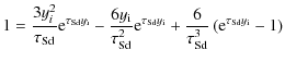
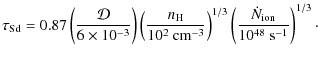
where we define the gas consumption timescale
| (13) |
We will refer to this form of the SFR as ``exponentially decaying''. In order to examine the effects of continuous (not decaying) input of ionizing photons, we also adopt another functional form for the SFR called ``constant SFR'':
We stop the calculation at
5.2 Evolution of ionizing photon luminosity
The evolution of the number of ionizing photons emitted per unit time,
![]() ,
is calculated by (HH06)
,
is calculated by (HH06)
| (15) |
where
5.3 Radius of the ionized region
In order to treat the range of evolution variations from deeply embedded H II regions to normal H II regions, it is crucial to include pressure-driven expansion of H II regions. We adopt a simple analytical approximation based on HH06. Here, we newly include the effect of dust, since A04 have shown that the dust extinction significantly reduces the radius of compact H IIregion.
We divide the growth of an H II region into two
stages: the first stage is the growth of the ionizing front
due to the increase of ionizing photons, and the second
is the pressure-driven expansion of ionized gas. The
expansion speed of the ionizing front in the first stage
is simply estimated by the increasing rate of the
ionization radius (Eq. (5)). We denote the
Strömgren radius under the initial density as
![]() ,
which is estimated by using
Eq. (1) with
,
which is estimated by using
Eq. (1) with
![]() .
Because of dust extinction, the ionization radius
.
Because of dust extinction, the ionization radius ![]() is reduced by a factor of
is reduced by a factor of ![]() ,
which is determined by solving Eq. (4), where
,
which is determined by solving Eq. (4), where
![]() is evaluated by Eq. (7) with a given
is evaluated by Eq. (7) with a given
![]() (or
(or ![]() ). The ionization radius
). The ionization radius ![]() and
and
![]() are estimated by Eqs. (5) and (6), respectively.
are estimated by Eqs. (5) and (6), respectively.
Initially, the increase of ![]() is caused by
the accumulation of ionizing stars. Roughly speaking,
as long as
is caused by
the accumulation of ionizing stars. Roughly speaking,
as long as
![]() (the increase rate of the ionization radius) is larger than the sound speed of ionized gas,
(the increase rate of the ionization radius) is larger than the sound speed of ionized gas,
![]() (we assume
(we assume
![]() km s-1 in this paper), the ionizing front propagates before the system responds hydrodynamically. Therefore,
we neglect the hydrodynamical expansion if
km s-1 in this paper), the ionizing front propagates before the system responds hydrodynamically. Therefore,
we neglect the hydrodynamical expansion if
![]() ,
and adopt the fixed density
,
and adopt the fixed density
![]() .
.
| Figure 5:
Time evolution of the number of ionizing photons emitted per unit time (
|
|
| Open with DEXTER | |
Once
![]() is satisfied,
pressure-driven expansion is treated. Since the density
evolves, we calculate the Strömgren radius
is satisfied,
pressure-driven expansion is treated. Since the density
evolves, we calculate the Strömgren radius ![]() under the current density
under the current density ![]() by using
Eq. (1). In this situation, the growth of the ionizing region
is governed by the pressure of ionized gas and the
luminosity change of the central stars has only a minor
effect. Therefore, the following equation derived by
assuming a constant luminosity (A04) approximately holds:
by using
Eq. (1). In this situation, the growth of the ionizing region
is governed by the pressure of ionized gas and the
luminosity change of the central stars has only a minor
effect. Therefore, the following equation derived by
assuming a constant luminosity (A04) approximately holds:
![$\displaystyle \left(\frac{\dot{r_{\rm i}}}{C_{\rm II}}\right)^2
=\frac{\rho_{\r...
...left[1-
\frac{\rho_{\rm II}}{\rho_{\rm I}}g(\tau_{\rm di})^{-2}
\right]^{-1}~ ,$](/articles/aa/full_html/2009/45/aa12020-09/img157.png)
where
| (17) |
The density ratio
![$\displaystyle \frac{\rho_{\rm II}}{\rho_{\rm I}} \simeq
\left(\frac{r_{\rm i0}}...
...^2)}
{-2+{\rm e}^{\tau_{\rm di}}
(2-2\tau_{\rm di}+\tau_{\rm di}^2)}
\right]~ ,$](/articles/aa/full_html/2009/45/aa12020-09/img163.png)
where
| (19) |
where
| (20) |
Equations (16) and (18) are numerically integrated to obtain
The above pressure-driven expansion is treated as long
as
![]() .
When the SFR declines significantly,
.
When the SFR declines significantly, ![]() begins to decrease. Thus,
begins to decrease. Thus,
![]() may be satisfied at a certain time. When
may be satisfied at a certain time. When
![]() ,
,
![]() is adopted with fixed
is adopted with fixed ![]() ;
that is, we finish treating the dynamical expansion.
;
that is, we finish treating the dynamical expansion.
6 Initial conditions and results
6.1 Active and passive star formation
We have argued in previous papers that star formation at
low metallicities can proceed in two ways:
one ``active'' mode in which stars form in dense, compact
complexes, and the other ``passive'' mode where star formation occurs
over more diffuse and extended regions. The size-density relation presented here for extragalactic H II regions naturally lends itself to the active/passive dichotomy (see also Hunt et al. 2003).
Dense regions tend also to be compact, while less dense ones
are more extended.
Here we examine these ``active'' and ``passive'' cases.
In HH06, SBS 0335-052 was used as a prototype of the ``active'' mode,
while I Zw 18 the ``passive'' one.
This representation was based mainly on the radio continuum results
for both galaxies (Hunt et al. 2004; Hunt et al. 2005).
Their linear emission measures differ by 3 orders of magnitude,
and the resulting densities by a factor of 10.
However, even in the optical, the electron densities inferred
from the [S II] line ratios differ by a factor of 5 or so
(SBS 0335-052 has
![]() -600 cm-3,
and I Zw 18
-600 cm-3,
and I Zw 18
![]() -120 cm-3, see
Table 2). The
-120 cm-3, see
Table 2). The
![]() of SBS 0335-052 calculated in this paper
(Table 2) is much lower than that adopted
in HH06 (
of SBS 0335-052 calculated in this paper
(Table 2) is much lower than that adopted
in HH06 (
![]() -600 cm-3; Izotov et al. 1999). As mentioned in Sect. 2 (see also Kennicutt 1984; Rozas et al. 1998), because of clumpiness the densities from the [S II] lines tend to be significantly higher than the
-600 cm-3; Izotov et al. 1999). As mentioned in Sect. 2 (see also Kennicutt 1984; Rozas et al. 1998), because of clumpiness the densities from the [S II] lines tend to be significantly higher than the
![]() .
The ``active'' nature of some BCDs therefore may not emerge in the
optical, at least with the rms densities we have adopted here. However,
if a BCD can be classified as ``active'', when observed in the radio,
it would have a compact, dense (or ultra-dense) H II region (see also Sect. 6.2).
.
The ``active'' nature of some BCDs therefore may not emerge in the
optical, at least with the rms densities we have adopted here. However,
if a BCD can be classified as ``active'', when observed in the radio,
it would have a compact, dense (or ultra-dense) H II region (see also Sect. 6.2).
![\begin{figure}
\par\mbox{\includegraphics[height=3.5cm]{12020fig6a.eps}\includeg...
...m]{12020fig6d.eps}\includegraphics[height=3.5cm]{12020fig6f.eps} }\end{figure}](/articles/aa/full_html/2009/45/aa12020-09/img174.png)
|
Figure 6:
Time evolution of the ionization radius ( |
| Open with DEXTER | |
![\begin{figure}
\par\hbox{\includegraphics[height=6cm,clip]{12020fig7a.eps}\hspace{-0.2cm}
\includegraphics[height=6cm,clip]{12020fig7b.eps} }
.
\end{figure}](/articles/aa/full_html/2009/45/aa12020-09/img175.png)
|
Figure 7:
Relation between the rms electron number density
|
| Open with DEXTER | |
Here, for consistency, we examine ``active'' and ``passive'' cases by
adopting similar initial conditions to those in HH06:
the active case is modelled by the so-called ``compact model'',
and the passive one by the ``diffuse model''.
Appropriate initial densities are
![]() -104 cm-3 for the compact model and
-104 cm-3 for the compact model and
![]() cm-3for the diffuse model (HH06). In addition, we also
adopt a denser model as a ``super-active'' class to explain the
extragalactic radio sample, and call this model the ``dense model''.
For all cases, the gas mass is fixed as
cm-3for the diffuse model (HH06). In addition, we also
adopt a denser model as a ``super-active'' class to explain the
extragalactic radio sample, and call this model the ``dense model''.
For all cases, the gas mass is fixed as
![]() ,
which is similar to the value adopted in HH06. We calculate the
evolution of the size-density relation of ionized region for the
continuous/burst star-formation histories (Sect. 5.1).
,
which is similar to the value adopted in HH06. We calculate the
evolution of the size-density relation of ionized region for the
continuous/burst star-formation histories (Sect. 5.1).
We also examine the dependence on ![]() ,
by setting
,
by setting
![]() ,
0.1, and 1 for dust-free,
dust-poor, and dust-rich (Galactic dust-to-gas ratio) cases, respectively.
These cases also correspond to varying degrees of dust
inhomogeneity or gas filling factor, as described in Sect. 4.3.
The sizes and densities of H II regions with a dust content corresponding to
,
0.1, and 1 for dust-free,
dust-poor, and dust-rich (Galactic dust-to-gas ratio) cases, respectively.
These cases also correspond to varying degrees of dust
inhomogeneity or gas filling factor, as described in Sect. 4.3.
The sizes and densities of H II regions with a dust content corresponding to
![]() are not significantly affected by dust (i.e., the results are similar to the case with
are not significantly affected by dust (i.e., the results are similar to the case with ![]() ), except for the dense model as we discuss later in Sect. 7.1.
On the other hand, the effects of dust extinction can be
quite pronounced for
), except for the dense model as we discuss later in Sect. 7.1.
On the other hand, the effects of dust extinction can be
quite pronounced for
![]() .
.
6.1.1 Dense model
We adopt
![]() cm-3 (
cm-3 (
![]() yr) and
yr) and
![]() .
With these assumptions, the SFR
.
With these assumptions, the SFR
![]()
![]() yr-1. First we show the evolution of
yr-1. First we show the evolution of
![]() in
Fig. 5a for the exponentially decaying and constant SFRs. In both
SFR scenarios,
in
Fig. 5a for the exponentially decaying and constant SFRs. In both
SFR scenarios,
![]() increases as time passes and stars form.
increases as time passes and stars form.
We present the basic evolutionary behavior of the
size and density of H II regions, focusing on
the effect of dust, which is newly incorporated in
this paper. In Figs. 6a and b, we show
the time variation of the ionization radius and
of the density, respectively, for various ![]() in the exponentially decaying star formation
history. The cases with
in the exponentially decaying star formation
history. The cases with
![]() (no dust) are the
same as those investigated in HH06. The general behavior
of pressure-driven expansion is qualitatively similar
in all the dust-to-gas ratios, but quantitatively
different. The ionization radius decreases as
the dust-to-gas ratio increases, because of the
absorption of ionizing photons. The density
decreases more rapidly in the dustier case,
since the expansion speed normalized to the
ionization radius is larger (for a smaller regions,
the expansion at a given speed decreases the
density more rapidly). The evolution of
(no dust) are the
same as those investigated in HH06. The general behavior
of pressure-driven expansion is qualitatively similar
in all the dust-to-gas ratios, but quantitatively
different. The ionization radius decreases as
the dust-to-gas ratio increases, because of the
absorption of ionizing photons. The density
decreases more rapidly in the dustier case,
since the expansion speed normalized to the
ionization radius is larger (for a smaller regions,
the expansion at a given speed decreases the
density more rapidly). The evolution of ![]() and
and ![]() is quantitatively similar.
is quantitatively similar.
6.1.2 Compact model
We adopt
![]() (
(
![]() yr) and
yr) and
![]() ,
as before.
With these values for the compact model, the SFR
,
as before.
With these values for the compact model, the SFR
![]()
![]() yr-1. First we show the evolution of
yr-1. First we show the evolution of
![]() in Fig. 5b for the exponentially decaying and constant SFRs:
Up to
in Fig. 5b for the exponentially decaying and constant SFRs:
Up to ![]() Myr,
Myr,
![]() increases as stars form. For the exponentially decaying SFR, it begins to decrease at
increases as stars form. For the exponentially decaying SFR, it begins to decrease at ![]() Myr because of
the death of massive stars, while for the constant SFR, it becomes
asymptotically constant because the death of massive stars is compensated by their continuous birth.
Myr because of
the death of massive stars, while for the constant SFR, it becomes
asymptotically constant because the death of massive stars is compensated by their continuous birth.
We present the evolutionary behavior of the size and density of H II regions in Figs. 6c and d for the exponentially
decaying star formation history. These models show similar behavior to the dense models. The increase of ![]() and the decrease of
and the decrease of ![]() stop at a later stage of the evolution because of the exponential decay of the SFR.
stop at a later stage of the evolution because of the exponential decay of the SFR.
The temporal behavior in the constant star formation is very similar to
that in the exponentially decaying one. The difference is that ![]() and
and ![]() continue to decrease and increase, respectively, because the SFR does not decay.
continue to decrease and increase, respectively, because the SFR does not decay.
6.1.3 Diffuse model
For the initial density and the radius, we assume
![]() (
(
![]() yr) and
yr) and
![]() ,
as above. In this case, for the diffuse model,
the SFR
,
as above. In this case, for the diffuse model,
the SFR
![]()
![]() yr-1. The evolution of
yr-1. The evolution of
![]() is shown in Fig. 5c for the exponentially decaying and constant SFRs: around 12 Myr,
is shown in Fig. 5c for the exponentially decaying and constant SFRs: around 12 Myr,
![]() is, respectively,
is, respectively,
![]() s-1 and
s-1 and
![]() s-1. The behavior of
s-1. The behavior of
![]() in the diffuse models as a
function of time is qualitatively the same as that in the compact models
(Sect. 6.1.2), but with a different SFR. We present the basic evolutionary behavior of the size and density of H II regions for the diffuse
models with various dust-to-gas ratios in Figs. 6e and f for the exponentially decaying star formation history. The cases with
in the diffuse models as a
function of time is qualitatively the same as that in the compact models
(Sect. 6.1.2), but with a different SFR. We present the basic evolutionary behavior of the size and density of H II regions for the diffuse
models with various dust-to-gas ratios in Figs. 6e and f for the exponentially decaying star formation history. The cases with ![]() (no dust) are the same as those investigated in HH06. For the
dependence on the dust-to-gas ratio, the same qualitative discussion as
in
Sect. 6.1.2 holds.
(no dust) are the same as those investigated in HH06. For the
dependence on the dust-to-gas ratio, the same qualitative discussion as
in
Sect. 6.1.2 holds.
The increase of ![]() and the decrease of
and the decrease of ![]() stop
for the same reason as in the compact models. The time evolution in the
constant star formation history is very similar to those in the
exponentially decaying one, but
stop
for the same reason as in the compact models. The time evolution in the
constant star formation history is very similar to those in the
exponentially decaying one, but ![]() and
and ![]() do not stop decreasing and increasing, respectively.
do not stop decreasing and increasing, respectively.
6.2 Evolutionary tracks on the size-density relation
In Figs. 7a
and b, we show the time
evolution of the ionized region on the size-density diagram for the
exponentially decaying SFR and the constant SFR, respectively.
For comparison with the data, we show the diameter of the ionized
region, ![]() :
:
| (21) |
Below we discuss the results of the three models.
6.2.1 Specific models
We observe from Fig. 7 that the dense models reproduce the data points of the radio sample.
This means that the radio sample can be understood as an extension of
the ``active'' mode of star formation toward higher density. However,
if a Galactic dust-to-gas ratio (
![]() )
is assumed, the predicted sizes are smaller than those of the radio
sample. This implies that the effects of dust extinction are suppressed
because of an intrinsically low dust content, a relatively high gas
filling factor, or a non-homogeneous dust distribution, but in a way
that is not strictly related to metallicity.
)
is assumed, the predicted sizes are smaller than those of the radio
sample. This implies that the effects of dust extinction are suppressed
because of an intrinsically low dust content, a relatively high gas
filling factor, or a non-homogeneous dust distribution, but in a way
that is not strictly related to metallicity.
Our models are based on the same gas mass, 107 ![]() ,
in the
dense, compact, and diffuse models. This implies that the star formation
activity traced by the radio sample cannot be neglected compared with that traced by the HST (optical) sample. As shown later in Sect. 7.1, the fraction of ionizing photons absorbed by
dust tends to be larger in denser regions. Thus, although they are potentially important to the total star formation
activity, compact and dense H II regions such as we have assembled in the radio sample would tend to be overlooked because of dust extinction.
,
in the
dense, compact, and diffuse models. This implies that the star formation
activity traced by the radio sample cannot be neglected compared with that traced by the HST (optical) sample. As shown later in Sect. 7.1, the fraction of ionizing photons absorbed by
dust tends to be larger in denser regions. Thus, although they are potentially important to the total star formation
activity, compact and dense H II regions such as we have assembled in the radio sample would tend to be overlooked because of dust extinction.
| Figure 8:
Evolution of
|
|
| Open with DEXTER | |
Figure 7 shows that the evolutionary tracks of the compact models in the size-density diagram explain the upper part
of the HST sample with ages of ![]() 3 Myr. Thus, the size and
density of the ``active'' class can be explained with the initial conditions of the compact model, while as shown below, those of the ``passive'' class can be reproduced with the less dense initial conditions of the diffuse model.
This is consistent with the picture that ``active'' and ``passive''
star formation processes originate from dense and diffuse SF
regions, respectively (Hirashita & Hunt 2004; HH06).
3 Myr. Thus, the size and
density of the ``active'' class can be explained with the initial conditions of the compact model, while as shown below, those of the ``passive'' class can be reproduced with the less dense initial conditions of the diffuse model.
This is consistent with the picture that ``active'' and ``passive''
star formation processes originate from dense and diffuse SF
regions, respectively (Hirashita & Hunt 2004; HH06).
The different classes are also distinguished by different
effects of dust extinction. This is shown in Fig. 8, which presents the evolution of the dust optical depth,
![]() ,
for the different classes of models. It can be seen that
,
for the different classes of models. It can be seen that
![]() is not a linear function of
is not a linear function of ![]() ;
if
;
if ![]() increases,
increases,
![]() increases with a fixed values of
increases with a fixed values of ![]() and
and
![]() (Eq. (7)), but
(Eq. (7)), but ![]() decreases (Eq. (3)). As a result, the product
decreases (Eq. (3)). As a result, the product
![]() is subject to these competing effects. In particular, if
is subject to these competing effects. In particular, if
![]() ,
this nonlinearity becomes significant. This is why
,
this nonlinearity becomes significant. This is why
![]() changes only by a factor of 8 under a change of
changes only by a factor of 8 under a change of ![]() by two orders of magnitude in
the dense model. In other words, if dust extinction dominates, the
size-density relation is expected to be aligned on a strip with
by two orders of magnitude in
the dense model. In other words, if dust extinction dominates, the
size-density relation is expected to be aligned on a strip with
![]() ,
although we should also consider the possibility that some
diffuse regions have low dust optical depth if
,
although we should also consider the possibility that some
diffuse regions have low dust optical depth if
![]() is appropriate.
is appropriate.
6.2.2 Summary of the evolutionary tracks
By examining the above three cases, we have inferred that very compact dense H II regions such as the radio sample, compact H II regions in ``active'' BCDs, and diffuse H II regions in ``passive'' BCDs are different populations which have emerged because of different initial densities. Our models also suggest that denser regions suffer more from the effects of dust than less dense ones; as shown in Fig. 8, ``active'' and ``passive'' star formation modes are characterized by different dust optical depths.
Contrary to the expectation at the end of Sect. 4.4, the radio and HST extragalactic samples cannot be reproduced with a single initial condition. Rather we should consider that we are seeing an ``envelope'' of individual evolutionary tracks of H II regions with diverse initial densities. The concept of ``envelope'' naturally suggests that we selectively observe the end points of the evolution: i.e., we tend to sample ``active'' SF regions with young ages of an order of Myr, while we observe ``passive'' regions with 10 Myr or older ages. In this sense, the observed size-density relation of extragalactic H II regions can be taken as an age sequence, although the relation contains different populations starting from different initial densities. The extreme youth of ``super-active'' (extremely dense) regions is also supported by the typical rising thermal radio spectrum from free-free gas absorption (Cannon & Skillman 2004; HH06; HH06 also argue that the initial density is important for the rising spectrum).
As mentioned before (Sect. 3.2), some of the galaxies in the HST sample are also present in the radio sample, as (ultra-)dense radio H II
regions. Hence, it may not only be a question of evolution, but rather
also of what the observations are probing. It seems that the more
finely some H II regions are probed, the smaller and more dense they appear, even in the same source. The H II region in NGC 5253 has a density of 7500-40 000 cm-3 if observed with a radio interferometer, but ![]() 300 cm-3 with an optical spectrum. The same is true for
He 2-10 (3300-10 000 cm-3 in the radio and
300 cm-3 with an optical spectrum. The same is true for
He 2-10 (3300-10 000 cm-3 in the radio and
![]() 500 cm-3 in the optical; Vacca & Conti 1992), II Zw 40 (35 000 cm-3 in the radio and
500 cm-3 in the optical; Vacca & Conti 1992), II Zw 40 (35 000 cm-3 in the radio and ![]() 190 cm-3 in the optical), and, as mentioned above, SBS 0335-052 (1500-7900 cm-3 in the radio
and
190 cm-3 in the optical), and, as mentioned above, SBS 0335-052 (1500-7900 cm-3 in the radio
and ![]() 500-600 cm-3 in the optical). Thus, we propose that there is a hierarchy of size and density. This picture is consistent
with that proposed by Kim & Koo (2001), Efremov & Elmegreen (1998) and Elmegreen (2000), and will be
further discussed in Sect. 7.4.
500-600 cm-3 in the optical). Thus, we propose that there is a hierarchy of size and density. This picture is consistent
with that proposed by Kim & Koo (2001), Efremov & Elmegreen (1998) and Elmegreen (2000), and will be
further discussed in Sect. 7.4.
7 Discussion
Here we discuss the implications of our results for evaluating star-formation activity from ionizing photons, and examine how the radio and HST samples fit into the larger picture of star formation locally and at high redshift.
7.1 The effects of dust
Even in the dust-poor case with
![]() ,
the absorption of ionizing photons by dust is significant,
especially in dense regions with
,
the absorption of ionizing photons by dust is significant,
especially in dense regions with
![]() cm-3 (see Fig. 7). The effect of dust extinction in the HST sample is expected to be smaller than in the radio sample,
but it is never negligible according to our results
if
cm-3 (see Fig. 7). The effect of dust extinction in the HST sample is expected to be smaller than in the radio sample,
but it is never negligible according to our results
if
![]() .
Thus, dust extinction could constrain the size of H II regions in BCDs, just as it does in Galactic H II regions.
.
Thus, dust extinction could constrain the size of H II regions in BCDs, just as it does in Galactic H II regions.
The most straightforward way to confirm if dust extinction
significantly alters the size-density relation is to overplot
on the data the dust optical depth calculated by the models in Sect. 4. For this purpose, we fix the expression for
![]() (Eq. (6)) to a constant, and then use the appropriate model
(Eq. (6)) to a constant, and then use the appropriate model
![]() and radius (
and radius (![]() )
which would give that
)
which would give that
![]() as an asymptotic value. This is done in Fig. 9 for
as an asymptotic value. This is done in Fig. 9 for
![]() ,
7, and 10 for
,
7, and 10 for ![]() and
and
![]() for
for
for
for
![]() ,
0.1, and 1. This is a similar diagram to Fig. 4, but with the difference that there we corrected the ionized gas column densities assuming a linear dependence on metallicity.
As for Fig. 4,
,
0.1, and 1. This is a similar diagram to Fig. 4, but with the difference that there we corrected the ionized gas column densities assuming a linear dependence on metallicity.
As for Fig. 4,
![]() was calculated for densities
which varied from 10-2 to 106 cm-3, and
was calculated for densities
which varied from 10-2 to 106 cm-3, and
![]() from 1048 to 1053 s-1; this is the reason that the lines of constant
from 1048 to 1053 s-1; this is the reason that the lines of constant
![]() do not extend over all radii and densities.
do not extend over all radii and densities.
![\begin{figure}
\par\hbox{\includegraphics[height=6cm]{12020fig9a.ps}\hspace{-0.2cm}
\includegraphics[height=6cm]{12020fig9b.ps} }\vspace*{3mm}
\end{figure}](/articles/aa/full_html/2009/45/aa12020-09/img204.png)
|
Figure 9:
Size-density relation with a constant dust
optical depth
|
| Open with DEXTER | |
With a fixed value of ![]() ,
large
,
large ![]() and/or large
and/or large ![]() are necessary to increase the dust optical depth
are necessary to increase the dust optical depth
![]() .
Thus, increasing
.
Thus, increasing
![]() moves the line of constant dust optical depth
upward and to the right. However,
a small value of
moves the line of constant dust optical depth
upward and to the right. However,
a small value of ![]() with a fixed
with a fixed
![]() shifts the line of constant
shifts the line of constant
![]() in the same direction,
because for a small value
of
in the same direction,
because for a small value
of ![]() ,
,
![]() and/or
and/or ![]() need to increase in order to
keep
need to increase in order to
keep
![]() constant. Therefore, the line of constant dust optical
depth depends strongly on the adopted value of
constant. Therefore, the line of constant dust optical
depth depends strongly on the adopted value of ![]() .
.
Several salient points emerge from Fig. 9, and from
the comparison of Figs. 9 and 4.
First, dust is an important factor in most of the H II regions in our sample, both Galactic and extragalactic ones,
since
![]() is indicated. While in Galactic H II regions, this is well established (e.g., Gail & Sedlmayr 1979; Melnick 1979; Churchwell et al. 1990), in low-metallicity BCDs the effects of dust have generally been thought to be negligible.
is indicated. While in Galactic H II regions, this is well established (e.g., Gail & Sedlmayr 1979; Melnick 1979; Churchwell et al. 1990), in low-metallicity BCDs the effects of dust have generally been thought to be negligible.
The second point is that in Fig. 9 the data
are fairly well approximated by different values of constant
![]() (except for the extremely compact and dense radio sample).
Figure 8 shows that
(except for the extremely compact and dense radio sample).
Figure 8 shows that
![]() predicted by our evolutionary
models varies by no more than a factor of two over the gas
consumption lifetime. This relative constancy of
predicted by our evolutionary
models varies by no more than a factor of two over the gas
consumption lifetime. This relative constancy of
![]() predicted by our models may be one of the main underlying factors in the size-density
relation observed in H II regions.
predicted by our models may be one of the main underlying factors in the size-density
relation observed in H II regions.
Thirdly, the correction for metal abundance applied in
Fig. 4 does not align the samples (see Sect. 3). The only difference between Figs. 9 and 4 is the correction for
metallicity assuming that
![]() metallicity.
The implication is that this correction is not valid,
namely that the dust-to-gas
ratio is not linear with metallicity (see also
Lisenfeld & Ferrara 1998;
Hirashita et al. 2002).
metallicity.
The implication is that this correction is not valid,
namely that the dust-to-gas
ratio is not linear with metallicity (see also
Lisenfeld & Ferrara 1998;
Hirashita et al. 2002).
Finally, the dense (radio) sample can only be approximated by
small values of
![]() .
Because the mean metal abundance of the radio sample is
.
Because the mean metal abundance of the radio sample is ![]() 0.22
0.22 ![]() ,
this low value of
,
this low value of ![]() cannot reflect a low dust-to-gas ratio resulting
from a linear variation with metallicity.
Instead, it must point either to regions evacuated of dust through
stellar winds, or to an intrinsic lack of dust perhaps because of
extreme youth. In addition, a relatively high gas filling factor or
an inhomogeneous dust distribution with a central cavity could
contribute to the small
cannot reflect a low dust-to-gas ratio resulting
from a linear variation with metallicity.
Instead, it must point either to regions evacuated of dust through
stellar winds, or to an intrinsic lack of dust perhaps because of
extreme youth. In addition, a relatively high gas filling factor or
an inhomogeneous dust distribution with a central cavity could
contribute to the small ![]() .
It is likely that all of these alternatives are shaping the properties
of these extreme H II regions.
.
It is likely that all of these alternatives are shaping the properties
of these extreme H II regions.
The generally high values of
![]() which are consistent with our
H II-region samples suggest the possibility that the size of many H II regions is limited by dust absorption of ionizing photons, rather than the
consumption of ionizing photons by neutral hydrogen.
If dust extinction governs the size of the H II region (we call this situation ``extinction-limited''),
we would naturally expect a constant column density
of H II
regions, which is equivalent to a constant dust optical depth under a
fixed mass absorption coefficient of dust grains. Natta & Panagia (1976) also derive a dust optical depth of order unity in the Lyman continuum from Galactic H II regions.
which are consistent with our
H II-region samples suggest the possibility that the size of many H II regions is limited by dust absorption of ionizing photons, rather than the
consumption of ionizing photons by neutral hydrogen.
If dust extinction governs the size of the H II region (we call this situation ``extinction-limited''),
we would naturally expect a constant column density
of H II
regions, which is equivalent to a constant dust optical depth under a
fixed mass absorption coefficient of dust grains. Natta & Panagia (1976) also derive a dust optical depth of order unity in the Lyman continuum from Galactic H II regions.
| Figure 10:
Evolution of f (the fraction of ionizing
photons absorbed by hydrogen). The solid, dotted, and dashed dotted lines present the results with
|
|
| Open with DEXTER | |
To further quantify the effects of dust extinction in our
models, we examine the fraction of ionizing photons
absorbed by hydrogen. This fraction is denoted as f and
the fraction of ionizing photons absorbed by dust
becomes 1-f. By using ![]() determined in
Eq. (4), f is expressed as (Spitzer 1978)
determined in
Eq. (4), f is expressed as (Spitzer 1978)
| (22) |
In Fig. 10, we show the evolution of f for the dense, compact, and diffuse models. It is clear that more than half of the ionizing photons are absorbed by dust even with
However, as noted in Sect. 4.2,
inhomogeneities in the dust distribution
affect f (
![]() ), which may be
larger (smaller) if we consider, for example, a central dust cavity
(Natta & Panagia 1976;
Inoue 2002). If such a cavity forms
efficiently on a timescale of
), which may be
larger (smaller) if we consider, for example, a central dust cavity
(Natta & Panagia 1976;
Inoue 2002). If such a cavity forms
efficiently on a timescale of ![]() 105 yr in
compact H II regions, f may increase and
the above underestimate of the mass of massive stars
could be less severe. For further qualitative discussion,
one should treat a motion equation of dusty gas, which
is left for future work.
105 yr in
compact H II regions, f may increase and
the above underestimate of the mass of massive stars
could be less severe. For further qualitative discussion,
one should treat a motion equation of dusty gas, which
is left for future work.
In summary, the above estimates of
![]() and
f imply that the dust grains play a central role in
determining the ionization radius. In particular,
the small values of f in compact ionized regions
indicate that the effect of dust grains significantly
reduce the number of ionizing photons and the ionization
radius. This means that there could be a large fraction of
massive stars which are not traced with radio observations
or with hydrogen recombination lines.
and
f imply that the dust grains play a central role in
determining the ionization radius. In particular,
the small values of f in compact ionized regions
indicate that the effect of dust grains significantly
reduce the number of ionizing photons and the ionization
radius. This means that there could be a large fraction of
massive stars which are not traced with radio observations
or with hydrogen recombination lines.
7.2 Galactic H II regions
We have shown that the sequence of
extragalactic H II regions
cannot be understood
as a sequence with a constant
![]() but that it can
be interpreted as an ``envelope'' of various
evolutionary tracks starting from diverse initial
densities. This may also be true for Galactic H II regions. Some Galactic H II regions are
associated with a single massive star, but some may be
associated with a forming stellar cluster, for which
we can apply the evolution model described in
Sect. 5. This may be the reason
why a similar size-density relation (
but that it can
be interpreted as an ``envelope'' of various
evolutionary tracks starting from diverse initial
densities. This may also be true for Galactic H II regions. Some Galactic H II regions are
associated with a single massive star, but some may be
associated with a forming stellar cluster, for which
we can apply the evolution model described in
Sect. 5. This may be the reason
why a similar size-density relation (
![]() )
fits the Galactic H II regions (Fig. 2).
)
fits the Galactic H II regions (Fig. 2).
In any case,
in agreement with previous work,
our models with constant
![]() suggest that
dust plays an important role in Galactic H II regions.
As shown in Fig. 9, the more compact H II regions are well fit by
suggest that
dust plays an important role in Galactic H II regions.
As shown in Fig. 9, the more compact H II regions are well fit by
![]() ,
while the less
compact ones by
,
while the less
compact ones by
![]() .
Hence, the Galactic H II region sequence could be a sequence of constant
.
Hence, the Galactic H II region sequence could be a sequence of constant
![]() .
Nevertheless, because high values of
.
Nevertheless, because high values of
![]() are only possible with high densities and large
are only possible with high densities and large
![]() ,
it could be that the most obscured regions are also the most intrinsically luminous, as suggested above.
,
it could be that the most obscured regions are also the most intrinsically luminous, as suggested above.
7.3 ``Active'' and ``passive'' BCDs
In Sect. 6, we have shown that it is not possible to reproduce the entire sample of extragalactic H II regions with a single initial condition. Indeed, the two ``active''/``passive'' star-formation modes proposed by Hunt et al. (2003) and elaborated upon in subsequent papers (Hirashita & Hunt 2004, HH06), could naturally result from different initial densities. The difference in the gas density (and the compactness) explains the variation in far-infrared luminosity and dust extinction (Takeuchi et al. 2003; Hirashita & Hunt 2004; Takeuchi et al. 2005) and in the molecular fraction (Hirashita & Hunt 2004) between the two classes. We had also hypothesized that the ``active'' class could be associated with the existence of SSCs. This is supported by the sizes and densities of the known SSCs in the Antennae galaxies (Gilbert & Graham 2007), which are well approximated by the compact models for the active mode of star formation.
In this paper, we have added the radio sample as a dense
extreme. The radio sample could be called
``super-active'' in the sense that their
H II regions are denser and more compact than even the ``active'' BCDs.
Indeed, our models imply that they constitute a
different population from the HST sample,
and that they are never detected in
the optical because of heavy dust extinction,
even at low values of ![]() .
Since a large number of
ionizing photons are absorbed by dust grains
(Sect. 7.1),
even the luminosity of the radio continuum or radio
recombination lines underestimates the
total mass of massive stars.
.
Since a large number of
ionizing photons are absorbed by dust grains
(Sect. 7.1),
even the luminosity of the radio continuum or radio
recombination lines underestimates the
total mass of massive stars.
The ``super-active'' mode of star formation seen in the
radio sample could also be consistent
with the idea that dense conditions foster the
formation of SSCs (Billett et al. 2002).
In fact, ultra-dense H II regions or radio ``supernebulae''
have been proposed as SSC progenitors, observed in
their very young embedded state (Kobulnicky & Johnson 1999; Johnson et al. 2003; Johnson et al. 2009). This would be consistent with our finding that extreme conditions are necessary to explain the radio sample.
The young age predicted by our models would also be consistent
with the age of ![]() 1 Myr derived from statistical
considerations by Kobulnicky & Johnson (1999).
1 Myr derived from statistical
considerations by Kobulnicky & Johnson (1999).
7.4 Density, time, and size in hierarchical star formation
Elmegreen and collaborators have proposed that there is
a timescale-size hierarchy in SF regions (Efremov & Elmegreen 1998; Elmegreen 2000, and references therein).
They found a relation between the time difference (![]() )
and
size and/or separation (S) of clouds and star clusters.
We have attempted to assess this trend for the HST sample
in Fig. 11
by plotting the H
)
and
size and/or separation (S) of clouds and star clusters.
We have attempted to assess this trend for the HST sample
in Fig. 11
by plotting the H![]() equivalent width (EW(H
equivalent width (EW(H![]() ))
against the diameter of the ELC as described above.
After about 3.1 Myr, EW(H
))
against the diameter of the ELC as described above.
After about 3.1 Myr, EW(H![]() )
linearly decreases with starburst
age (Leitherer et al. 1999), so we might expect a trend
between age and size to be traced by EW(H
)
linearly decreases with starburst
age (Leitherer et al. 1999), so we might expect a trend
between age and size to be traced by EW(H![]() )
and ELC diameter.
The figure shows a weak negative correlation, formally
)
and ELC diameter.
The figure shows a weak negative correlation, formally ![]()
![]() .
The two dashed lines, correspond to different methods
for determining slopes (Isobe et al. 1990):
minimizing the perpendicular distance to the line gives
.
The two dashed lines, correspond to different methods
for determining slopes (Isobe et al. 1990):
minimizing the perpendicular distance to the line gives
![]() ,
and the ordinary-least-squared (OLS) bisector,
,
and the ordinary-least-squared (OLS) bisector,
![]() .
The fitted intercepts at zero size correspond roughly to
.
The fitted intercepts at zero size correspond roughly to ![]() 1000 Å,
roughly the EW(H
1000 Å,
roughly the EW(H![]() )
``plateau'' for ages younger than
)
``plateau'' for ages younger than ![]() 3.1 Myr
at oxygen abundances 0.05
3.1 Myr
at oxygen abundances 0.05 ![]() .
The fitted power-law indices for the HST sample are very close to that found by
Efremov & Elmegreen (1998) and Elmegreen (2000)
of
.
The fitted power-law indices for the HST sample are very close to that found by
Efremov & Elmegreen (1998) and Elmegreen (2000)
of
![]() for molecular clouds and star clusters in the LMC. Hence, even in extragalactic H II regions, there is some (albeit weak) indication that
time and size are related, perhaps because of the imprinting of turbulent molecular cloud
fragmentation on the star clusters responsible for ionizing the H II gas.
for molecular clouds and star clusters in the LMC. Hence, even in extragalactic H II regions, there is some (albeit weak) indication that
time and size are related, perhaps because of the imprinting of turbulent molecular cloud
fragmentation on the star clusters responsible for ionizing the H II gas.
![\begin{figure}
\par\includegraphics[width=8cm,clip]{12020fig11.ps}
\end{figure}](/articles/aa/full_html/2009/45/aa12020-09/img216.png)
|
Figure 11:
H |
| Open with DEXTER | |
Indeed, the size-density relation of H II regions,
![]() ,
may be compatible with the above time-size relation.
Considering that the timescale of star formation
scales with the free-fall timescale
(see Sect. 5.1 and Elmegreen 2000),
it may be reasonable to assume a scaling relation
,
may be compatible with the above time-size relation.
Considering that the timescale of star formation
scales with the free-fall timescale
(see Sect. 5.1 and Elmegreen 2000),
it may be reasonable to assume a scaling relation
![]() .
Combining
these two density scaling relations, we obtain
.
Combining
these two density scaling relations, we obtain
![]() ,
as long
the typical size or separation of SF regions is determined by the size of ionizing radius,
,
as long
the typical size or separation of SF regions is determined by the size of ionizing radius,
![]() .
We would thus obtain
the same scaling relation as shown by Efremov & Elmegreen (1998) and Elmegreen (2000).
.
We would thus obtain
the same scaling relation as shown by Efremov & Elmegreen (1998) and Elmegreen (2000).
Although our data for H II regions cannot be used to determine star formation activity from small scales to large (galactic) scales (e.g., Elmegreen 2000), we would argue that pressure-driven expansion in H II regions and ionization of the surrounding medium can play a significant role in determining the typical extension or separation of SF complexes. Considering that the dust optical depth affects the ionization radius of H II regions, it is also possible that dust could be a main factor for determining the typical extension or separation of SF regions.
7.5 Implications for high-redshift star formation
The number density of gas in high-redshift primeval
galaxies is theoretically considered to be
![]() 103 cm-3(Norman & Spaans 1997). Therefore, the
SF regions in such galaxies
may be expected to mimic our compact models. This means
that a significant fraction of ionizing photons can
be absorbed by dust grains.
According to Fig. 10,
roughly 1/3 of the ionizing photons are absorbed
in the compact model even when
103 cm-3(Norman & Spaans 1997). Therefore, the
SF regions in such galaxies
may be expected to mimic our compact models. This means
that a significant fraction of ionizing photons can
be absorbed by dust grains.
According to Fig. 10,
roughly 1/3 of the ionizing photons are absorbed
in the compact model even when
![]() .
A pair-instability supernova originating from a Population III star is expected to supply
.
A pair-instability supernova originating from a Population III star is expected to supply ![]()
![]() of dust grains (Nozawa et al. 2003;
Schneider et al. 2004); if the baryonic mass of the first object is
of dust grains (Nozawa et al. 2003;
Schneider et al. 2004); if the baryonic mass of the first object is ![]()
![]() (Tegmark et al. 1997), the dust-to-gas
ratio becomes
(Tegmark et al. 1997), the dust-to-gas
ratio becomes ![]() 10-4 (
10-4 (
![]() ).
Thus,
).
Thus,
![]() is reached relatively quickly, and
dust extinction becomes important soon after
the death of the first Population III stars.
Our results also suggest that the radiative transfer
of ionizing photons at high z is strongly affected
by dust extinction. Thus, the cosmic reionization
history should be reconsidered by taking into
account the effects of dust extinction.
is reached relatively quickly, and
dust extinction becomes important soon after
the death of the first Population III stars.
Our results also suggest that the radiative transfer
of ionizing photons at high z is strongly affected
by dust extinction. Thus, the cosmic reionization
history should be reconsidered by taking into
account the effects of dust extinction.
It is also interesting to consider the starburst populations
at lower (but still high) redshifts (![]() ). Although resolving individual dense H II regions is impossible in high-zgalaxies, an intense starburst at high z would be expected to
produce several giant H II regions or massive ELCs.
For example, let us assume a star-forming region whose gas mass is three
orders of magnitude larger than that assumed for the
BCDs (i.e.,
). Although resolving individual dense H II regions is impossible in high-zgalaxies, an intense starburst at high z would be expected to
produce several giant H II regions or massive ELCs.
For example, let us assume a star-forming region whose gas mass is three
orders of magnitude larger than that assumed for the
BCDs (i.e.,
![]() ;
note that
this is not the total gas mass in the entire galaxy but
the gas mass involved in the current star formation episode).
With
;
note that
this is not the total gas mass in the entire galaxy but
the gas mass involved in the current star formation episode).
With
![]() (typical density for the diffuse model) we can roughly reproduce a typical SFR
(typical density for the diffuse model) we can roughly reproduce a typical SFR ![]()
![]() (Eq. (11))
for luminous infrared galaxies (Sanders & Mirabel 1996). If the exponentially decaying SFR is adopted, this model after
(Eq. (11))
for luminous infrared galaxies (Sanders & Mirabel 1996). If the exponentially decaying SFR is adopted, this model after ![]() Myr
can also be used to mimic a typical SFR of more mildly star-forming
populations such as Lyman break galaxies and Ly
Myr
can also be used to mimic a typical SFR of more mildly star-forming
populations such as Lyman break galaxies and Ly![]() emitters
(e.g., Takeuchi & Ishii 2004;
Pirzkal et al. 2007). Moreover, with
emitters
(e.g., Takeuchi & Ishii 2004;
Pirzkal et al. 2007). Moreover, with
![]() ,
the SFR
roughly becomes a typical value for such extreme
starbursts (
,
the SFR
roughly becomes a typical value for such extreme
starbursts (![]()
![]() )
as are
seen in submillimeter galaxies (e.g.,
Hughes et al. 1998).
)
as are
seen in submillimeter galaxies (e.g.,
Hughes et al. 1998).
Because the Strömgren radius depends only weakly on
![]() (Eq. (2)), the size of H II regions is only one order of magnitude larger even when
the SFR (
(Eq. (2)), the size of H II regions is only one order of magnitude larger even when
the SFR (
![]() is proportional to SFR) increases by
three orders of magnitude.
Severe dust extinction would lessen the increase of H II region
size. Nevertheless, this implies that high-zstarburst population could produce an immense dense H II region whose size (
is proportional to SFR) increases by
three orders of magnitude.
Severe dust extinction would lessen the increase of H II region
size. Nevertheless, this implies that high-zstarburst population could produce an immense dense H II region whose size (![]() 100 pc) is an order of
magnitude larger than the local (dense) extragalactic H II regions.
100 pc) is an order of
magnitude larger than the local (dense) extragalactic H II regions.
In these massive H II regions, if the H II region
size becomes larger than 100 pc, pressure-driven
expansion ceases to be important. The reason is as follows:
pressure-driven expansion
occurs on a sound-crossing timescale. Since the
sound speed in H II regions is ![]() 10 km s-1,
the sound-crossing time over a 100 pc region is
10 Myr, comparable to the typical lifetime of massive
stars. Thus, such a giant H II region cannot be sustained
long enough for the pressure-driven expansion to
modify the ionized-gas density. Consequently, the density of such a giant H II region reflects the initial density averaged over the current H II region size.
10 km s-1,
the sound-crossing time over a 100 pc region is
10 Myr, comparable to the typical lifetime of massive
stars. Thus, such a giant H II region cannot be sustained
long enough for the pressure-driven expansion to
modify the ionized-gas density. Consequently, the density of such a giant H II region reflects the initial density averaged over the current H II region size.
7.6 Maximum-intensity starbursts
The ``dense'' (``super-active'') and ``active'' star formation
modes we have modelled far exceed the empirical global star-formation
intensity limit of ![]() 45
45 ![]() yr-1 kpc-2found by Meurer et al. (1997).
However, recent observations of submillimeter galaxies and quasar hosts
at high redshift have discovered ``hyper-starbursts'' occurring in
small regions of
yr-1 kpc-2found by Meurer et al. (1997).
However, recent observations of submillimeter galaxies and quasar hosts
at high redshift have discovered ``hyper-starbursts'' occurring in
small regions of ![]() 1-3 kpc in diameter
(e.g., Tacconi et al. 2006; Walter et al. 2009).
These kiloparsec-scale starbursts have SFRs per unit area
on the order of 100-1000
1-3 kpc in diameter
(e.g., Tacconi et al. 2006; Walter et al. 2009).
These kiloparsec-scale starbursts have SFRs per unit area
on the order of 100-1000 ![]() yr-1 kpc-2,
comparable to those of our models. Similar high starburst surface
densities are found in Arp 220 but on spatial scales of a few
100 pc (Scoville et al. 1997). With 1010
yr-1 kpc-2,
comparable to those of our models. Similar high starburst surface
densities are found in Arp 220 but on spatial scales of a few
100 pc (Scoville et al. 1997). With 1010 ![]() of gas, roughly that in Arp 220,
these are roughly the spatial extents predicted by our evolutionary
models for massive starbursts, as described in the previous section.
of gas, roughly that in Arp 220,
these are roughly the spatial extents predicted by our evolutionary
models for massive starbursts, as described in the previous section.
If dust is a principle factor in shaping the observable properties of H II regions and ELCs, then we might expect shorter wavelengths, in particular the ultraviolet, to be unsuitable for sampling SFRs in such objects. This would mean that starburst intensity limits both locally and at high redshift would need to be reassessed at submillimeter or infrared wavelengths where dust reprocessing gives a more accurate picture (see also Gao 2008).
8 Conclusions
We have investigated the size-density relation of extragalactic H II regions, focusing on those in BCDs. Motivated by the similarity of size-density relations of extragalactic H II regions with Galactic ones, we have modelled and examined the size-density relation of ionized regions by considering the effects of dust, star formation history, and pressure-driven expansion of H II regions. The results have been compared with several samples spanning roughly six orders of magnitude in size and density. We have shown that the entire sample set cannot be understood as an evolutionary sequence with a single initial condition. Rather, the size-density relation reflects a sequence with different initial gas densities. Thus, a hierarchical structure of SF regions with various densities is implied.
We have also found that the size of extragalactic
H II regions is ``dust-extinction limited'', in the sense
that the dust absorption of ionizing photons is significant.
This naturally explains the observed size-density
relation of H II regions as following a constant column
density of ionized gas, if the dust-to-gas ratio in
H II
regions is constant. The dust extinction of ionizing photons is
particularly severe over the entire lifetime of the compact radio
sample
with typical densities of ![]() 103 cm-3.
This means that the compact radio sample constitutes a
different population from the optical samples and that
star formation activity in such dense regions would be
underestimated or missed entirely if we use the emission from H II regions (hydrogen recombination lines, free-free
continuum) as the sole indicators of star formation rate.
103 cm-3.
This means that the compact radio sample constitutes a
different population from the optical samples and that
star formation activity in such dense regions would be
underestimated or missed entirely if we use the emission from H II regions (hydrogen recombination lines, free-free
continuum) as the sole indicators of star formation rate.
We would like to humbly dedicate this paper to the memory of Prof. Edwin Salpeter, who provided precious insight during its development. We are also grateful to B. G. Elmegreen, R. C. Kennicutt, and A. K. Inoue for stimulating discussions on the properties of H II regions. Finally, we thank the anonymous referee for useful comments which substantially improved the paper. This research has made use of the NASA/IPAC Extragalactic Database (NED), which is operated by the Jet Propulsion Laboratory, California Institute of Technology, under contract with the National Aeronautics and Space Administration (NASA).
Appendix A: Simple derivation of Eq. (7)
Equation (7) is derived in Hirashita et al. (2001) based on Spitzer (1978). Here, we present a simpler derivation of Eq. (7).
We start from the optical depth at the threshold wavelength of the Lyman continuum (912 Å) denoted as
![]() :
:
| (A.1) |
where
| (A.2) |
for solar metallicity. Then we obtain
| (A.3) |
Next, we estimate
References
- Anderson, L. D., & Bania, T. M. 2009, ApJ, 690, 706 [NASA ADS] [CrossRef]
- Anders, E., & Grevesse, N. 1989, Geochim. Cosmochim. Acta, 53, 197 [NASA ADS] [CrossRef]
- Arthur, S. J., Kurtz, S. E., Franco, J., et al. 2004, ApJ, 608, 282 [NASA ADS] [CrossRef] (A04)
- Beck, S. C., Turner, J. L., & Kovo, O. 2000, AJ, 120, 244 [NASA ADS] [CrossRef]
- Beck, S. C., Turner, J. L., Langland-Shula, L. E., et al. 2002, AJ, 124, 2516 [NASA ADS] [CrossRef]
- Billett, O. H., Hunter, D. A., & Elmegreen, B. G. 2002, AJ, 123, 1454 [NASA ADS] [CrossRef]
- Buckalew, B. A., Kobulnicky, H. A., & Dufour, R. J. 2005, ApJS, 157, 30 [NASA ADS] [CrossRef]
- Cannon, J. M., & Skillman, E. D. 2004, ApJ, 610, 772 [NASA ADS] [CrossRef]
- Churchwell, E., & Goss, W. M. 1999, ApJ, 514, 188 [NASA ADS] [CrossRef]
- Churchwell, E., Wolfire, M. G., & Wood, D. O. S. 1990, ApJ, 354, 247 [NASA ADS] [CrossRef]
- Corbin, M. R., Vacca, W. D., Hibbard, J. E., et al. 2005, ApJ, 629, L89 [NASA ADS] [CrossRef]
- Deeg, H.-J., Brinks, E., Duric, N., Klein, U., & Skillman, E. 1993, ApJ, 410, 626 [NASA ADS] [CrossRef]
- Dopita, M. A., Fischera, J., Crowley, O., et al. 2006, ApJ, 639, 788 [NASA ADS] [CrossRef]
- Efremov, Y. N., & Elmegreen, B. G. 1998, MNRAS, 299, 588 [NASA ADS] [CrossRef]
- Elmegreen, B. G. 2000, ApJ, 530, 277 [NASA ADS] [CrossRef]
- Foster, T., & MacWilliams, J. 2006, ApJ, 644, 214 [NASA ADS] [CrossRef]
- Freedman, W. L., Wilson, C. D., & Madore, B. F. 1991, ApJ, 372, 455 [NASA ADS] [CrossRef]
- Gail, H. P., & Sedlmayr, E. 1979, A&A, 77, 165 [NASA ADS]
- Gao, Y. 2008, Nature, 452, 417 [NASA ADS] [CrossRef]
- Garay, G., & Lizano, S. 1999, PASP, 111, 1049 [NASA ADS] [CrossRef]
- Garnett, D. R. 2002, ApJ, 581, 1019 [NASA ADS] [CrossRef]
- Giammanco, C., Beckman, J. E., Zurita, A., et al. 2004, A&A, 424, 877 [NASA ADS] [CrossRef] [EDP Sciences]
- Gies, D. R., & Lambert, D. L. 1992, ApJ, 387, 673 [NASA ADS] [CrossRef]
- Gilbert, A. M., & Graham, J. R. 2007, ApJ, 668, 168 [NASA ADS] [CrossRef]
- Gordon, M. A. 1988, Galactic and Extragalactic Radio Astronomy, 37
- Guseva, N. G., Izotov, Y. I., & Thuan, T. X. 2000, ApJ, 531, 776 [NASA ADS] [CrossRef]
- Guseva, N. G., Papaderos, P., Izotov, Y. I., et al. 2003, A&A, 407, 105 [NASA ADS] [CrossRef] [EDP Sciences]
- Guseva, N. G., Papaderos, P., Izotov, Y. I., et al. 2004, A&A, 421, 519 [NASA ADS] [CrossRef] [EDP Sciences]
- Guseva, N. G., Izotov, Y. I., Papaderos, P., et al. 2007, A&A, 464, 885 [NASA ADS] [CrossRef] [EDP Sciences]
- Hachisuka, K., Brunthaler, A., Menten, K. M., et al. 2006, ApJ, 645, 337 [NASA ADS] [CrossRef]
- Hirashita, H., & Hunt, L. K. 2004, A&A, 421, 555 [NASA ADS] [CrossRef] [EDP Sciences]
- Hirashita, H., & Hunt, L. K. 2006, A&A, 460, 67 [NASA ADS] [CrossRef] [EDP Sciences] (HH06)
- Hirashita, H., Inoue, A. K., Kamaya, H., et al. 2001, A&A, 366, 83 [NASA ADS] [CrossRef] [EDP Sciences]
- Hirashita, H., Tajiri, Y. Y., & Kamaya, H. 2002, A&A, 388, 439 [NASA ADS] [CrossRef] [EDP Sciences]
- Hughes, D. H., Serjeant, S., Dunlop, J., et al. 1998, Nature, 394, 241 [NASA ADS] [CrossRef]
- Hunt, L. K., Vanzi, L., & Thuan, T. X. 2001, A&A, 377, 66 [NASA ADS] [CrossRef] [EDP Sciences]
- Hunt, L. K., Hirashita, H., Thuan, T. X., Izotov, Y. I., & Vanzi, L. 2003, in Proceedings of Galaxy Evolution: Theory and Observations, ed. V. Avila-Reese, C. Firmani, C. Frenk, & C. Allen, Rev. Mex. Astron. Astrofis. Ser. Conf. [arXiv:astro-ph/0310865]
- Hunt, L. K., Dyer, K. K., Thuan, T. X., et al. 2004, ApJ, 606, 853 [NASA ADS] [CrossRef]
- Hunt, L. K., Dyer, K. K., & Thuan, T. X. 2005, A&A, 436, 837 [NASA ADS] [CrossRef] [EDP Sciences]
- Hunter, D. A., & Hoffman, L. 1999, AJ, 117, 2789 [NASA ADS] [CrossRef]
- Inoue, A. K. 2002, ApJ, 570, 688 [NASA ADS] [CrossRef]
- Inoue, A. K., Hirashita, H., & Kamaya, H. 2001, ApJ, 555, 613 [NASA ADS] [CrossRef]
- Isobe, T., Feigelson, E. D., Akritas, M. G., et al. 1990, ApJ, 364, 104 [NASA ADS] [CrossRef]
- Izotov, Y. I., & Thuan, T. X. 1998, ApJ, 500, 188 [NASA ADS] [CrossRef]
- Izotov, Y. I., & Thuan, T. X. 2004, ApJ, 602, 200 [NASA ADS] [CrossRef]
- Izotov, Y. I., Thuan, T. X., & Lipovetsky, V. A. 1994, ApJ, 435, 647 [NASA ADS] [CrossRef]
- Izotov, Y. I., Thuan, T. X., & Lipovetsky, V. A. 1997, ApJS, 108, 1 [NASA ADS] [CrossRef]
- Izotov, Y. I., Chaffee, F. H., Foltz, C. B., et al. 1999, ApJ, 527, 757 [NASA ADS] [CrossRef]
- Izotov, Y. I., Chaffee, F. H., Foltz, C. B., et al. 2001a, ApJ, 566, 222 [NASA ADS] [CrossRef]
- Izotov, Y. I., Chaffee, F. H., & Green, R. F. 2001b, ApJ, 562, 727 [NASA ADS] [CrossRef]
- Izotov, Y. I., Papaderos, P., Guseva, N. G., et al. 2004, A&A, 421, 539 [NASA ADS] [CrossRef] [EDP Sciences]
- Izotov, Y. I., Schaerer, D., Blecha, A., et al. 2006a, A&A, 459, 71 [NASA ADS] [CrossRef] [EDP Sciences]
- Izotov, Y. I., Stasinska, G., Meynet, G., et al. 2006b, A&A, 448, 955 [NASA ADS] [CrossRef] [EDP Sciences]
- Izotov, Y. I., Thuan, T. X., & Stasinska, G. 2007, ApJ, 662, 15 [NASA ADS] [CrossRef]
- Johnson, K. E., Leitherer, C., Vacca, W. D., et al. 2000, AJ, 120, 1273 [NASA ADS] [CrossRef]
- Johnson, K. E., Kobulnicky, H. A., Massey, P., et al. 2001, ApJ, 559, 864 [NASA ADS] [CrossRef]
- Johnson, K. E., Indebetouw, R., & Pisano, D. J. 2003, AJ, 126, 101 [NASA ADS] [CrossRef]
- Johnson, K. E., Hunt, L. K., & Reines, A. E. 2009, AJ, 137, 3788 [NASA ADS] [CrossRef]
- Kehrig, C., Vílchez, J. M., Telles, E., et al. 2006, A&A, 457, 477 [NASA ADS] [CrossRef] [EDP Sciences]
- Kennicutt, R. C., Jr. 1984, ApJ, 287, 116 [NASA ADS] [CrossRef]
- Kim, K.-T., & Koo, B.-C. 2001, ApJ, 549, 979 [NASA ADS] [CrossRef]
- Kilian, J. 1992, A&A, 262, 171 [NASA ADS]
- Kitayama, T., Yoshida, N., Susa, H., et al. 2004, ApJ, 613, 631 [NASA ADS] [CrossRef]
- Kniazev, A. Y., Pustilnik, S. A., Masegosa, J., et al. 2000, A&A, 357, 101 [NASA ADS]
- Kniazev, A. Y., Pustilnik, S. A., Ugryumov, A. V., et al. 2001, A&A, 371, 404 [NASA ADS] [CrossRef] [EDP Sciences]
- Kobulnicky, H. A., & Skillman, E. D. 1996, ApJ, 471, 211 [NASA ADS] [CrossRef]
- Kobulnicky, H. A., & Johnson, K. E. 1999, ApJ, 527, 154 [NASA ADS] [CrossRef]
- Kobulnicky, H. A., Kennicutt, R. C., Jr., & Pizagno, J. L. 1999, ApJ, 514, 544 [NASA ADS] [CrossRef]
- Kunth, D., & Joubert, M. 1985, A&A, 142, 411 [NASA ADS]
- Larson, R. B. 1981, MNRAS, 194, 809 [NASA ADS]
- Leitherer, C., Schaerer, D., Goldader, J. D., et al. 1999, ApJS, 123, 3 [NASA ADS] [CrossRef]
- Lequeux, J., & Viallefond, F. 1980, A&A, 91, 269 [NASA ADS]
- Lisenfeld, U., & Ferrara, A. 1998, ApJ, 496, 145 [NASA ADS] [CrossRef]
- Martín-Hernández, N. L., van der Hulst, J. M., & Tielens, A. G. G. M. 2003, A&A, 407, 957 [NASA ADS] [CrossRef] [EDP Sciences]
- Martín-Hernández, N. L., Vermeij, R., & van der Hulst, J. M. 2005, A&A, 433, 205 [NASA ADS] [CrossRef] [EDP Sciences]
- Massey, P., & Hunter, D. A. 1998, ApJ, 493, 180 [NASA ADS] [CrossRef]
- Mathis, J. S. 2000, in Allen's Astrophysical Quantities, Fourth Edition, ed. A. N. Cox (New York: Springer), 523
- Melnick, J. 1979, ApJ, 228, 112 [NASA ADS] [CrossRef]
- Mohan, N. R., Anantharamaiah, K. R., & Goss, W. M. 2001, ApJ, 557, 659 [NASA ADS] [CrossRef]
- Moustakas, J., & Kennicutt, R. C., Jr. 2006, ApJS, 164, 81 [NASA ADS] [CrossRef]
- Meurer, G. R., Heckman, T. M., Lehnert, M. D., Leitherer, C., & Lowenthal, J. 1997, AJ, 114, 54 [NASA ADS] [CrossRef]
- Mezger, P. G., & Henderson, A. P. 1967, ApJ, 147, 471 [NASA ADS] [CrossRef]
- Natta, A., & Panagia, N. 1976, A&A, 50, 191 [NASA ADS]
- Norman, C. A., & Spaans, M. 1997, ApJ, 480, 145 [NASA ADS] [CrossRef]
- Nozawa, T., Kozasa, T., Umeda, H., et al. 2003, ApJ, 598, 785 [NASA ADS] [CrossRef]
- Noeske, K. G., Guseva, N. G., Fricke, K. J., et al. 2000, A&A, 361, 33 [NASA ADS]
- Omukai, K., & Nishi, R. 1999, ApJ, 518, 64 [NASA ADS] [CrossRef]
- Osterbrock, D., & Flather, E. 1959, ApJ, 129, 26 [NASA ADS] [CrossRef]
- Osterbrock, D. E., & Ferland, G. J. 2006, Astrophysics of Gaseous Nebulae and Active Galactic Nuclei, Second edn (Sausalito: University Science Books)
- Papaderos, P., Guseva, N. G., Izotov, Y. I., et al. 2006, A&A, 457, 45 [NASA ADS] [CrossRef] [EDP Sciences]
- Peimbert, M. 1987, in Star Forming Regions, ed. M. Peimbert, & J. Jugaku (Dordrecht: Reidel), 111
- Petrosian, V., Silk, J., & Field, G. B. 1972, ApJ, 177, L69 [NASA ADS] [CrossRef]
- Pirzkal, N., Malhotra, S., Rhoads, J. E., et al. 2007, ApJ, 667, 49 [NASA ADS] [CrossRef]
- Reines, A. E., Johnson, K. E., & Hunt, L. K. 2008, AJ, 136, 1415 [NASA ADS] [CrossRef]
- Rozas, M., Castaneda, H. O., & Beckman, J. E. 1998, A&A, 330, 873 [NASA ADS]
- Russeil, D., Adami, C., & Georgelin, Y. M. 2007, A&A, 470, 161 [NASA ADS] [CrossRef] [EDP Sciences]
- Salpeter, E. E. 1955, ApJ, 121, 161 [NASA ADS] [CrossRef]
- Sanders, D. B., & Mirabel, I. F. 1996, ARA&A, 34, 749 [NASA ADS] [CrossRef]
- Schaerer, D. 2002, A&A, 382, 28 [NASA ADS] [CrossRef] [EDP Sciences]
- Schneider, R., Ferrara, A., & Salvaterra, R. 2004, MNRAS, 351, 1379 [NASA ADS] [CrossRef]
- Scoville, N. Z., Yun, M. S., & Bryant, P. M. 1997, ApJ, 484, 702 [NASA ADS] [CrossRef]
- Shi, F., Kong, X., Li, C., et al. 2005, A&A, 437, 849 [NASA ADS] [CrossRef] [EDP Sciences]
- Silich, S., Tenorio-Tagle, G., & Muñoz-Tuñón, C. 2007, ApJ, 669, 952 [NASA ADS] [CrossRef]
- Spitzer, L., Jr. 1978, Physical Processes in the Interstellar Medium (New York: Wiley)
- Tacconi, L. J., Neri, R., Chapman, S. C., et al. 2006, ApJ, 640, 228 [NASA ADS] [CrossRef]
- Takeuchi, T. T., & Ishii, T. T. 2004, A&A, 426, 425 [NASA ADS] [CrossRef] [EDP Sciences]
- Takeuchi, T. T., Hirashita, H., Ishii, T. T., Hunt, L. K., & Ferrara, A. 2003, MNRAS, 343, 839 [NASA ADS] [CrossRef]
- Takeuchi, T. T., Ishii, T. T., Nozawa, T., et al. 2005, MNRAS, 362, 592 [NASA ADS] [CrossRef]
- Tegmark, M., Silk, J., Rees, M. J., et al. 1997, ApJ, 474, 1 [NASA ADS] [CrossRef]
- Tenorio-Tagle, G., Muñoz-Tuñón, C., Pérez, E., Silich, S., & Telles, E. 2006, ApJ, 643, 186 [NASA ADS] [CrossRef]
- Thuan, T. X., & Izotov, Y. I. 2005, ApJS, 161, 240 [NASA ADS] [CrossRef]
- Thuan, T. X., Izotov, Y. I., & Lipovetsky, V. A. 1996, ApJ, 463, 120 [NASA ADS] [CrossRef]
- Thuan, T. X., Izotov, Y. I., & Lipovetsky, V. A. 1997, ApJ, 477, 661 [NASA ADS] [CrossRef]
- Thuan, T. X., Sauvage, M., & Madden, S. 1999, ApJ, 516, 783 [NASA ADS] [CrossRef]
- Turner, J. L., Beck, S. C., & Ho, P. T. P. 2000, ApJ, 532, L109 [NASA ADS] [CrossRef]
- Vacca, W. D., & Conti, P. S. 1992, ApJ, 401, 543 [NASA ADS] [CrossRef]
- Vanzi, L., Hunt, L. K., & Thuan, T. X. 2002, A&A, 390, 481 [NASA ADS] [CrossRef] [EDP Sciences]
- Walsh, J. R., & Roy, J.-R. 1989, MNRAS, 239, 297 [NASA ADS]
- Walter, F., Riechers, D., Cox, P., et al. 2009, Nature, 457, 699 [NASA ADS] [CrossRef]
- Yoshida, N., Abel, T., Hernquist, L., et al. 2003, ApJ, 592, 645 [NASA ADS] [CrossRef]
- Zaritsky, D., Kennicutt, R. C., Jr., & Huchra, J. P. 1994, ApJ, 420, 87 [NASA ADS] [CrossRef]
Footnotes
- ...

![[*]](/icons/foot_motif.png)
- In this and future relative solar abundances, we will adopt the solar calibration of Anders & Grevesse (1989).
- ...
Archive
- The Hubble Legacy Archive is a collaboration between the Space Telescope Science Institute (STScI/NASA), the Space Telescope European Coordinating Facility (ST-ECF/ESA) and the Canadian Astronomy Data Centre (CADC/NRC/CSA).
- ... coefficient
- This value is for a gas temperature of T=10 000 K (Spitzer 1978; Osterbrock & Ferland 2006). If we adopt T=8000 K and 20 000 K, we find
 and
and
 cm3 s-1, respectively. The temperature dependence of
 does not change our conclusions as long as we assume a typical gas temperature
  10 000 K in H II regions.
- ... lines
- In our static model,
the corrected column densities correspond to
 cm-2, assuming a Galactic dust-to-gas ratio of
 (see Appendix A).
All Tables
Table 1: Radio sample.
Table 2: HST sample.
All Figures
|
|
Figure 1:
Rms densities
|
| Open with DEXTER | |
| In the text | |
|
|
Figure 2:
Densities |
| Open with DEXTER | |
| In the text | |
|
|
Figure 3:
Relation between the rms electron number density
|
| Open with DEXTER | |
| In the text | |
|
|
Figure 4:
Ionized gas column densities (cm-2)
vs. diameter (pc). The ionized gas column densities have been
multiplied by their oxygen abundance relative to solar, assuming the
Anders & Grevesse (1989) calibration. Constant
|
| Open with DEXTER | |
| In the text | |
| |
Figure 5:
Time evolution of the number of ionizing photons emitted per unit time (
|
| Open with DEXTER | |
| In the text | |
|
|
Figure 6:
Time evolution of the ionization radius ( |
| Open with DEXTER | |
| In the text | |
|
|
Figure 7:
Relation between the rms electron number density
|
| Open with DEXTER | |
| In the text | |
| |
Figure 8:
Evolution of
|
| Open with DEXTER | |
| In the text | |
|
|
Figure 9:
Size-density relation with a constant dust
optical depth
|
| Open with DEXTER | |
| In the text | |
| |
Figure 10:
Evolution of f (the fraction of ionizing
photons absorbed by hydrogen). The solid, dotted, and dashed dotted lines present the results with
|
| Open with DEXTER | |
| In the text | |
|
|
Figure 11:
H |
| Open with DEXTER | |
| In the text | |
Copyright ESO 2009
Current usage metrics show cumulative count of Article Views (full-text article views including HTML views, PDF and ePub downloads, according to the available data) and Abstracts Views on Vision4Press platform.
Data correspond to usage on the plateform after 2015. The current usage metrics is available 48-96 hours after online publication and is updated daily on week days.
Initial download of the metrics may take a while.