| Issue |
A&A
Volume 507, Number 2, November IV 2009
|
|
|---|---|---|
| Page(s) | 949 - 967 | |
| Section | The Sun | |
| DOI | https://doi.org/10.1051/0004-6361/200912394 | |
| Published online | 11 August 2009 | |
A&A 507, 949-967 (2009)
Magnetic flux emergence into the solar photosphere and chromosphere
A. Tortosa-Andreu1 - F. Moreno-Insertis1,2
1 - Instituto de Astrofísica de Canarias (IAC), La
Laguna (Tenerife), Spain
2 - Department of Astrophysics, Faculty of Physics, Universidad de La
Laguna (Tenerife), Spain
Received 27 April 2009 / Accepted 24 June 2009
Abstract
Aims. We model the emergence of magnetized plasma
across granular convection cells and the low atmosphere, including
layers up to the mid-chromosphere.
Methods. Three-dimensional numerical experiments are
carried out in which the equations of MHD and radiative transfer are
solved self-consistently. We use the MURaM code, which assumes local
thermodynamic equilibrium between plasma and radiation.
Results. In the photosphere, we find good agreement
between our simulation predictions and observational results obtained
with the Hinode satellite for the velocity and magnetic fields. We also
confirm earlier simulation results by other authors. Our experiments
reveal a natural mechanism of formation of twisted magnetic flux tubes
that results from the retraction of photospheric horizontal fields at
new intergranular lanes in decaying granules. In the chromosphere, we
present evidence for the non-radiative heating of the emerging
magnetized plasma due to the passage of shocks and/or ohmic
dissipation. We study the formation of high-temperature points in the
magnetic domain. We detect two types of points, classified according to
whether they have a photospheric counterpart or otherwise. We also find
evidence of those two types in Hinode observations.
Using Lagrangian tracing of a large statistical sample of fluid particles, we detect and study episodes of convective collapse of magnetic elements returning to the photosphere. On the other hand, we study the maximum heights reached by all tracers, magnetized or otherwise. Only a small fraction (1.3%) of the magnetic elements reach the mid-chromosphere (z>750 km), while virtually no unmagnetized elements in the sample rise above the level of the reverse granulation (a few 100 km above the photosphere). We find that the rise into the chromosphere occurs in the form of successive jumps with intermediate stops rather than in a smooth continuous fashion and propose a tentative explanation of this behavior. Finally, also using Lagrange tracing, we document the creation of high-temperature points in the chromosphere via rising shock fronts.
Key words: Sun: magnetic fields - Sun: chromosphere - Sun: photosphere - magnetohydrodynamics (MHD) - radiative transfer - Sun: granulation
1 Introduction
The emergence of magnetized plasma into the solar atmosphere after traversing the turbulent convection cells below the surface is one of the basic processes that determine the structure and dynamics of the observable domains of the Sun. Magnetic bipoles and, more generally, magnetic regions emerge from the solar interior on a wide range of length- and timescales, stretching from those of the largest activity complexes, with horizontal sizes comparable to the depth of the entire convection zone, through those of intermediate-sized active regions and ephemeral regions down to small-scale, granule-sized emergence events (as recently observed with Hinode/SOT by Martinez Gonzalez & Bellot Rubio 2009; Centeno et al. 2007; Ishikawa et al. 2008; Orozco Suárez et al. 2008; Otsuji et al. 2007). Observationally, the use of Stokes polarimetry and the achievement of subarcsecond resolution in both ground-based and space observations have provided a wealth of knowledge concerning the emergence of magnetic field on different scales and at individual heights (additionally to the references just mentioned, see the papers by Lites et al. 1995; Martinez Pillet et al. 1994; De Pontieu 2002; Kubo et al. 2003; Harvey et al. 2007; Lites et al. 1998; Okamoto et al. 2008; Shimizu et al. 2008; Nagata et al. 2008; Lites 2009; van Driel-Gesztelyi & Culhane 2009). Yet, when rising, the magnetized plasma straddles the extremely inhomogeneous region constituted by the photosphere, chromosphere, and transition region, where density and pressure change by more than eight orders of magnitude in only a few Mm in height and temperature goes from photospheric values up to a million K in the corona. To observe a flux emergence event in its entirety one would need quasi-simultaneous measurements with detectors in the visible/IR, (E)UV, and X-ray ranges. This, and the stochastic nature of the flux emergence events, make it very difficult to put together a comprehensive observational picture of the flux emergence phenomenon.
The theoretical effort, on the other hand, has advanced using large 2D or 3D computer models of the emergence process that include the uppermost layers of the convection zone and a range of heights in the atmosphere. Two classes of models can be distinguished: a first branch includes the levels from a few Mm at the top of the convection zone all the way up to the corona. To ensure that the computing speed and data analysis are within reasonable bounds, these models strongly simplify the thermodynamics of the plasma by ignoring its interaction with the radiation field ; in most cases, heat conduction is also ignored (see as representative examples, e.g., Fan 2001; Galsgaard et al. 2005; Shibata et al. 1989; Kusano et al. 1998; Magara & Longcope 2001; Matsumoto et al. 1993; Galsgaard et al. 2007; Archontis et al. 2005; Matsumoto et al. 1998; Abbett & Fisher 2003; Arber et al. 2007; Archontis et al. 2004; Manchester 2001; Murray et al. 2009,2006; Magara & Longcope 2003; Moreno-Insertis et al. 2008; Nozawa et al. 1992; Manchester et al. 2004; Yokoyama & Shibata 1996; Matsumoto & Shibata 1992; Yokoyama & Shibata 1995; Miyagoshi & Yokoyama 2004). The neglect of the coupling with the radiation field in the energy equation limits the possibilities of detailed comparison with observational data in those regions where the radiative effects are important (most prominently the photosphere). On the positive side, these models lead to conclusions about phenomena such as the formation of current sheets at the interface between emerging and pre-existing flux systems in the atmosphere, field line reconnection, emission of high-speed, high-temperature jets in the corona, or plasmoid formation.
On the other hand, in the past few years a new generation of
flux emergence
models has appeared that solve the radiation transfer problem
simultaneously
with the MHD equations (Martínez-Sykora
et al. 2008; Cheung et al. 2008,2007a;
see also Dorch et al.
2001). In the two
papers by Cheung
et al., the domain considered
extends for 450 km and 300 km, respectively, above
the average
![]() level, whereas, in depth, the box extends for
1.85 Mm and 5.5 Mm, respectively. To start the
emergence
process, the authors planted a buoyant horizontal magnetic flux
tube in the lower levels of the domain. Cheung
et al. (2007a)
considered cases with different field intensities ranging from
8500 to 2500 G, different levels of field line twist and
magnetic flux between approximately
level, whereas, in depth, the box extends for
1.85 Mm and 5.5 Mm, respectively. To start the
emergence
process, the authors planted a buoyant horizontal magnetic flux
tube in the lower levels of the domain. Cheung
et al. (2007a)
considered cases with different field intensities ranging from
8500 to 2500 G, different levels of field line twist and
magnetic flux between approximately ![]() and
1019 Mx. When rising, the tubes of the
weakest field
intensity and lowest flux were strongly distorted by the
convective flows; upon reaching the surface, a salt-and-pepper
pattern of vertical magnetic elements with mixed polarities
resulted that had no simple bipolar region structure. On the other
hand, the cases with higher initial field strength and higher
total flux managed to distort the granulation pattern: a series of
abnormally large and dark granules appeared when the magnetic
domain reached the photosphere; these anomalous granules were
arranged along a lane that reflects the geometry of the initial
magnetic tube. In the later paper by Cheung
et al. (2008), the
tube had an initial total flux
and
1019 Mx. When rising, the tubes of the
weakest field
intensity and lowest flux were strongly distorted by the
convective flows; upon reaching the surface, a salt-and-pepper
pattern of vertical magnetic elements with mixed polarities
resulted that had no simple bipolar region structure. On the other
hand, the cases with higher initial field strength and higher
total flux managed to distort the granulation pattern: a series of
abnormally large and dark granules appeared when the magnetic
domain reached the photosphere; these anomalous granules were
arranged along a lane that reflects the geometry of the initial
magnetic tube. In the later paper by Cheung
et al. (2008), the
tube had an initial total flux ![]() Mx
with the
buoyancy concentrated in the center of the box. Hence, the tube
develops an
Mx
with the
buoyancy concentrated in the center of the box. Hence, the tube
develops an ![]() -loop
shape perturbed by the convective flows
and yields a globally bipolar magnetic region at the surface, even
though with a large amount of mixed polarity in its interior. A
wealth of further features amenable to comparison with actual
observations were obtained in these experiments, such as the
convective collapse of photospheric flux tubes, cancellation of
magnetic flux at the surface, and the existence of transient
kilogauss horizontal fields. In both papers, the simplification of
a gray atmosphere in local thermodynamic equilibrium (LTE) was
used to model the radiation transfer.
-loop
shape perturbed by the convective flows
and yields a globally bipolar magnetic region at the surface, even
though with a large amount of mixed polarity in its interior. A
wealth of further features amenable to comparison with actual
observations were obtained in these experiments, such as the
convective collapse of photospheric flux tubes, cancellation of
magnetic flux at the surface, and the existence of transient
kilogauss horizontal fields. In both papers, the simplification of
a gray atmosphere in local thermodynamic equilibrium (LTE) was
used to model the radiation transfer.
In the more recent work by Martínez-Sykora et al. (2008), the experiments are carried out over a large domain in the vertical direction, including 1.4 Mm below and 14.6 Mm above the photosphere. They, therefore, include chromosphere, transition region and an extended domain in the corona. The equation of radiation transfer is solved using the opacity binning method (Nordlund 1982) and includes coherent scattering in the continuum following the method developed by Skartlien (2000). Additionally, optically thin radiative losses in the upper chromosphere and corona were included in the energy equation by means of source terms based on precalculated functions, in part using the non-LTE dynamical chromospheric models of Carlsson & Stein (1997,2002). The authors inject magnetic flux through the lower boundary either in the form of a magnetic tube (with different levels of field line twist in different experiments) or of a magnetized horizontal sheet. Of particular relevance to the current paper are the results concerning the chromosphere: cold volumes develop coinciding with (in fact, appearing slightly before) the arrival of the magnetized plasma there; the chromosphere and the transition region are pushed upward by as much as 3-4 Mm by the emerging plasma; bright points are formed in the periphery of the rising tube both at photospheric and chromospheric heights, with high values of magnetic field intensity, vertical velocity and vorticity.
The current paper builds upon the work of Cheung et al. (2007a), enlarging the physical domain of the experiment to include chromospheric layers (more precisely, the low and middle chromosphere). The focus of this paper is a detailed study of the phenomena taking place at chromospheric heights during the emergence process as well as a comparison of the evolution in the different layers from the photosphere to the mid-chromosphere. The paper starts with a brief description of the emergence of flux at the photosphere, especially concerning the magnetically modified granulation and the statistics of the horizontal and vertical field components (Sects. 3.2 and 3.3). Of special interest is the discovery of the formation of horizontal twisted flux tubes in the subphotospheric layers right below the downflow lanes that appear across decaying granules (Sect. 3.4). The twisted tubes are created as a result of the submergence of horizontal photospheric fields effected by the downflow: a U-loop is formed in the subphotospheric levels, reconnection ensues and a twisted, roughly horizontal tube is formed.
The events at chromospheric heights are studied in detail in Sect. 4. The chromosphere prior to flux emergence in our experiment (Sect. 4.1) resembles in many respects the higher levels in the experiments of Wedemeyer et al. (2004), who studied the structure of the non-magnetic chromosphere with particular attention to its heating by means of rising shock fronts. In Sect. 4.2, three types of patterns developing in the flux emerging regions are described, namely: 1) extended cool patches, 2) hot filaments forming between adjacent regions, and 3) high-temperature points. Further subsections are devoted to the geometry and topology of the magnetic field from photosphere to chromosphere (Sect. 4.3), the heating of the magnetized plasma (Sect. 4.4), and the relation between chromospheric high-T points, downflows, and magnetic concentrations observed by Hinode (Sect. 4.5): we identify, both in simulations and observations, two types of chromospheric high-Tpoints that differ in the nature of their photospheric counterparts.
A statistical study of the evolution of individual plasma
elements
involved in the emergence process is carried out in
Sect. 5.
To this end, Lagrange tracers initially
located below the photosphere are used. Among other things, we
study the average height reached by magnetized and unmagnetized
elements in their rise (Sect. 5.2); we
find
that only a tiny minority of the initial tracers reach the
chromosphere (less than ![]() of the unmagnetized elements rise
above 200 km in the atmosphere; only about
of the unmagnetized elements rise
above 200 km in the atmosphere; only about ![]() of the
magnetized ones rise beyond 750 km in height). We also find
that
the magnetized elements reaching high levels in the chromosphere
do not rise in a continuous fashion but, instead, go through a
series of temporary stops along the rise. Finally, we show direct
evidence for the origin of the high-T points at
chromospheric
levels in terms of shock waves traveling upward in the middle of
the magnetized cool patches resulting from the emergence
(Sect. 5.3).
of the
magnetized ones rise beyond 750 km in height). We also find
that
the magnetized elements reaching high levels in the chromosphere
do not rise in a continuous fashion but, instead, go through a
series of temporary stops along the rise. Finally, we show direct
evidence for the origin of the high-T points at
chromospheric
levels in terms of shock waves traveling upward in the middle of
the magnetized cool patches resulting from the emergence
(Sect. 5.3).
2 Methods, numerical setup, and initial and boundary conditions
2.1 Equations and numerical tools
The numerical experiments in the present paper solve the equations of magnetohydrodynamics including radiation transfer. We use the customary MHD equations for the time evolution of the mass, momentum, and total energy densities and of the magnetic field (the induction equation). The equations include viscous and ohmic dissipation and a cooling term that corresponds to the exchange of energy between the plasma and the radiation field. The equations are solved using the MURaM code (Vögler et al. 2005), which includes 4th-order accurate spatial and time derivatives. The code also includes hyperdiffusivity algorithms to smooth discontinuous transitions, such as shocks. We use them for the viscous diffusion, while for the resistive terms the standard MHD expression is used. The radiation transfer problem is tackled by solving the radiation transfer equation,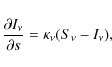
along 24 rays passing through each grid point. In Eq. (1), s is the arc-length along each given ray,
2.2 Initial and boundary conditions
We build the initial condition for the experiments in two steps, following the general scheme used by Cheung (2006). First, a non-magnetic model of stationary 3D convection is created that includes the topmost few megameters below the surface, the photosphere, and the low-mid chromospheric heights. We then introduce magnetic flux into the lower part of the box, which leads to the flux emergence episode.In the present paper, for the non-magnetic convection model we
use
a plane-parallel stratification using the 1D vertical profiles of
Spruit (1974) for the
interior and VALC (Vernazza
et al. 1981) for
the atmosphere. The size of the box in the horizontal directions
is 16 Mm ![]() 12 Mm (
12 Mm (
![]() ).
The
vertical size is 3.8 Mm, (1.2 Mm above,
2.6 Mm below the
solar surface). The surface, located at z=0, is
determined as
the level where the mean Rosseland optical depth is unity. The
grid spacing is set at 20 km (height) and 50 km
(horizontal),
so that the numerical grid has
).
The
vertical size is 3.8 Mm, (1.2 Mm above,
2.6 Mm below the
solar surface). The surface, located at z=0, is
determined as
the level where the mean Rosseland optical depth is unity. The
grid spacing is set at 20 km (height) and 50 km
(horizontal),
so that the numerical grid has ![]() points
in (x,y,z). To
promote the convective instability, white noise
at the
points
in (x,y,z). To
promote the convective instability, white noise
at the ![]() level is added to the specific internal energy in the
vertical range (-500,
10) km. The system is allowed to evolve
for 2 solar hours, yielding a thermally relaxed, statistically
stationary state for the convection.
level is added to the specific internal energy in the
vertical range (-500,
10) km. The system is allowed to evolve
for 2 solar hours, yielding a thermally relaxed, statistically
stationary state for the convection.
In the second step, a horizontal magnetic flux tube is added
to
the relaxed convection model. The tube axis is parallel to the
x-axis and is located 1.8 Mm below the
surface at y=0. The
field lines are twisted around the axis; using cylindrical
coordinates ![]() centered on the tube axis, the
longitudinal (
centered on the tube axis, the
longitudinal (![]() )
and azimuthal (
)
and azimuthal (![]() )
field
components are given by
)
field
components are given by
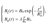
In Eq. (2), the parameter R0 provides a measure of the tube radius and
The plasma in the tube is made buoyant by modifying its entropy
and, consequently, its density. Two different cases are presented
in this paper, called S1 and S2 in the following (see
Table 1).
For S1, the horizontal-tube experiment, buoyancy is
imparted all along the length of
the tube, while the perturbation decreases the further one goes
away from the tube axis. To achieve that, the unperturbed entropy
distribution, s0(x,r)
is changed to: ![]() ,
where
,
where ![]() is the mean
specific entropy of the upflows at the position of the tube axis.
The buoyant tube is therefore expected to rise retaining a
globally horizontal shape, even if more or less distorted by the
convective flows. For S2, the
is the mean
specific entropy of the upflows at the position of the tube axis.
The buoyant tube is therefore expected to rise retaining a
globally horizontal shape, even if more or less distorted by the
convective flows. For S2, the ![]() -loop
case, the
buoyancy is concentrated in the central part of the tube and given
by
-loop
case, the
buoyancy is concentrated in the central part of the tube and given
by ![]() ,
where Lx=16 Mm
and
,
where Lx=16 Mm
and
![]() is the mean entropy for the downflows
near the visible surface (z=-50 km). The
part of the tube close
to x=0 is therefore underdense both with respect to
the flanks
and to the surrounding upflows and downflows. The tube then
evolves into an
is the mean entropy for the downflows
near the visible surface (z=-50 km). The
part of the tube close
to x=0 is therefore underdense both with respect to
the flanks
and to the surrounding upflows and downflows. The tube then
evolves into an ![]() -shaped
structure, where the top of the
-shaped
structure, where the top of the
![]() rises, its
feet slowly descend toward the boundaries of
the box.
rises, its
feet slowly descend toward the boundaries of
the box.
Table 1: Set of parameters for the initial magnetic flux tube in the runs described in the paper.
As boundary conditions, we adopt periodicity on the sides, an open boundary at the bottom (balancing mass outflow and inflow, to guarantee mass conservation, as done by Vögler et al. 2005 or Cheung 2006), and a closed, stress-free boundary at the top. For the magnetic field, a zero vertical derivative condition for the horizontal components and constant vertical derivative for Bz are imposed at the top and bottom boundary.
3 Evolution in the interior and in the photosphere
3.1 Initial stages: evolution in the interior
The initial properties of the magnetic tube, especially its initial field strength and twist, determine whether the rising magnetized plasma can resist the disrupting effect of the convective flows. Taking into account the local equipartition field strength with the convective flows (between 2 and 3 kG at z=-1.8 Mm) and on the basis of earlier estimates (Moreno-Insertis 1983; Fan et al. 2003; Cheung et al. 2007a), we expect our initial tube to be able to maintain its coherence along the rise, even if with a convectively perturbed shape. For both the S1 and S2 cases, the average upward velocity is![\begin{figure}
\par\scalebox{1}{\includegraphics[]{Version-electronique-RGB/eps/12394f01.eps}}\end{figure}](/articles/aa/full_html/2009/44/aa12394-09/img54.png)
|
Figure 1: Magnetized volume at the time of arrival of the magnetic flux at the surface (top: case S1; bottom: case S2). See explanations in the text (Sect. 3.1). Note that, for clarity, the vertical scale has been stretched. |
| Open with DEXTER | |
3.2 Flux evolution in the photosphere: anomalous granulation
Young unmagnetized granules in standard convection have a large pressure excess at their center that allows them to grow, pushing aside their neighbors (Stein & Nordlund 1998). When the incipient granule carries a magnetic field of sufficient intensity, the additional push of the magnetic pressure can be expected to lead to anomalous granules, i.e., larger than usual cells. This is indeed the case in our experiments and those of Cheung et al. (2007a) (strong case) and Cheung et al. (2008).
In run S1 (the horizontal tube experiment),
magnetized
granules first appear at the photosphere as isolated cells around
![]() min
(upper-left panel of Fig. 2), growing
to an abnormally large size (panels at 10.2 and
12.6 min in Fig. 2) with
horizontal expansion
velocity of 6-8 km s-1
(compared with
4-6 km s-1 for young normal
granules) and adopting an
elongated shape. The anomalous granules reach a peak total
pressure
min
(upper-left panel of Fig. 2), growing
to an abnormally large size (panels at 10.2 and
12.6 min in Fig. 2) with
horizontal expansion
velocity of 6-8 km s-1
(compared with
4-6 km s-1 for young normal
granules) and adopting an
elongated shape. The anomalous granules reach a peak total
pressure ![]() larger than for normal granules, the difference
being due basically to the magnetic pressure of the former.
larger than for normal granules, the difference
being due basically to the magnetic pressure of the former.
![\begin{figure}
\par\scalebox{0.28}{\includegraphics[]{Version-electronique-RGB/eps/12394f02.eps}}\vspace*{-1mm}
\vspace*{-2mm}
\end{figure}](/articles/aa/full_html/2009/44/aa12394-09/img57.png)
|
Figure 2:
Time evolution of the anomalous granulation for the S1 case. The gray
shading is a Dopplergram (i.e., a color map for vz)
at the |
| Open with DEXTER | |
At time ![]() min, the collection
of abnormal granules
covers a lane parallel to the x-direction
reflecting the initial
tube orientation apparent in the upper panel of
Fig. 1;
in Fig. 2,
one sees that the intervening unmagnetized granules have shrunk
and disappeared (compare the two leftmost panels); each anomalous
granule, in turn, is elongated in the y-direction.
This
anisotropy is due, first, to the competition between neighboring
magnetized cells: they have a comparable pressure excess, so that
the expansion in the direction away from the initial tube axis is
favored. Additionally, when reaching the surface, the rising
magnetic field points in the y-direction and the
Alfven Mach
number does not greatly exceed unity, so the Lorentz force tends
to align the flows along the y-axis. The anisotropy
is clearly
noticeable in the horizontal velocities: a histogram of the
azimuthal angle of
min, the collection
of abnormal granules
covers a lane parallel to the x-direction
reflecting the initial
tube orientation apparent in the upper panel of
Fig. 1;
in Fig. 2,
one sees that the intervening unmagnetized granules have shrunk
and disappeared (compare the two leftmost panels); each anomalous
granule, in turn, is elongated in the y-direction.
This
anisotropy is due, first, to the competition between neighboring
magnetized cells: they have a comparable pressure excess, so that
the expansion in the direction away from the initial tube axis is
favored. Additionally, when reaching the surface, the rising
magnetic field points in the y-direction and the
Alfven Mach
number does not greatly exceed unity, so the Lorentz force tends
to align the flows along the y-axis. The anisotropy
is clearly
noticeable in the horizontal velocities: a histogram of the
azimuthal angle of ![]() at this time (t=12.5 min)
shows two marked peaks of some 7 km s-1
in the positive and
negative y-direction. The average horizontal speed
in the
granule is 3.3 km s-1.
Non-magnetized granules, on the
other hand, have a fully isotropic distribution and the average
speed is
at this time (t=12.5 min)
shows two marked peaks of some 7 km s-1
in the positive and
negative y-direction. The average horizontal speed
in the
granule is 3.3 km s-1.
Non-magnetized granules, on the
other hand, have a fully isotropic distribution and the average
speed is ![]() km s-1.
km s-1.
The appearance of anomalous granulation in flux emergence
regions
can also be found in observational data. Anomalous, elongated
granules can be directly seen in the movie by
Hammerschlag
et al. (2007), compiled with G-band
spectral
filter 430-431 nm observations taken with the Dutch Open
Telescope (La Palma Spain). Our numerical results are also in
agreement with the recent Hinode observations of a flux emergence
episode by Otsuji
et al. (2007). They show the presence of
dark lanes of some ![]() in length at the flux emergence site
in the photosphere both in Stokes-I and in the G-band.
The
values just reported for the horizontal speed in the magnetized
domain (average: 3.3 km s-1;
peak: 7 km s-1) are
also compatible with the observed horizontal expansion of
3.8 km s-1.
in length at the flux emergence site
in the photosphere both in Stokes-I and in the G-band.
The
values just reported for the horizontal speed in the magnetized
domain (average: 3.3 km s-1;
peak: 7 km s-1) are
also compatible with the observed horizontal expansion of
3.8 km s-1.
The anomalous granules grow until about ![]() min,
reaching a
maximum size of
min,
reaching a
maximum size of ![]() 7.5 Mm2,
several times the average for
the non-magnetic granules. Thereafter, fragmentation sets in by
means of a mechanism as for normal granules: the upflow velocity
and energy transport to the surface decrease and some locations
start to show an excess of radiative cooling. There, a downflow
develops, and intergranular lanes form that cut across the
anomalous granular cell.
7.5 Mm2,
several times the average for
the non-magnetic granules. Thereafter, fragmentation sets in by
means of a mechanism as for normal granules: the upflow velocity
and energy transport to the surface decrease and some locations
start to show an excess of radiative cooling. There, a downflow
develops, and intergranular lanes form that cut across the
anomalous granular cell.
Run S2 (the ![]() -loop
case) also shows that the magnetic
granules are abnormally large, although now, naturally, they form
a cluster coinciding with the upper part of the
-loop
case) also shows that the magnetic
granules are abnormally large, although now, naturally, they form
a cluster coinciding with the upper part of the ![]() -loop
instead of a lane. The initial shape of the granules shows some
elongation in the direction of the magnetic field, but this
preference soon disappears; also, there is no privileged direction
for the expanding horizontal velocities. The total magnetized area
in the S2 experiment grows to occupy about 33 Mm2
some
15 min after the first appearance of the magnetic field at the
surface.
-loop
instead of a lane. The initial shape of the granules shows some
elongation in the direction of the magnetic field, but this
preference soon disappears; also, there is no privileged direction
for the expanding horizontal velocities. The total magnetized area
in the S2 experiment grows to occupy about 33 Mm2
some
15 min after the first appearance of the magnetic field at the
surface.
3.3 Horizontal and vertical magnetic field in the photosphere
![\begin{figure}
\par\includegraphics[width=9cm,clip]{Version-electronique-RGB/eps/12394f03.eps} %
\vspace*{2mm}\vspace*{3mm}
\end{figure}](/articles/aa/full_html/2009/44/aa12394-09/img63.png)
|
Figure 3:
Horizontal and vertical fields in the emerging flux
region. The PDFs correspond to the horizontal field (green) and
vertical field (red) at two heights: |
| Open with DEXTER | |
In spite of the buffeting and distortion by the subsurface flows, we expect the magnetic field at the forefront of the rising magnetic domain to be oriented preferentially in the horizontal direction. This follows in part from the initial field distribution, but also from the predominance of the expansion in the horizontal directions along the rise. There is ample evidence in the literature for the relevance of horizontal fields in emerging flux regions, both from observations (Lites 2009; Lites et al. 1996,1998; Harvey et al. 2007) and numerical experiments (Cheung et al. 2008,2007a). Recently, using Hinode data, different groups have also detected horizontal fields in small-scale emergence episodes (Martinez Gonzalez & Bellot Rubio 2009; Centeno et al. 2007; Ishikawa et al. 2008; Otsuji et al. 2007).
In our experiment, when the magnetized plasma first arrives at
the
surface yielding the large and elongated granules discussed in
Sect. 3.2,
we indeed find that the magnetic field
is predominantly horizontal. The PDFs of
Fig. 3,
drawn for ![]() (middle
row of panels) and z=200 km (bottom row)
illustrate the
situation. The green and red curves in them show the number of
pixels for a given |B | where
(middle
row of panels) and z=200 km (bottom row)
illustrate the
situation. The green and red curves in them show the number of
pixels for a given |B | where ![]() (green)
or viceversa (red). The green curves (horizontal fields)
at time 10.2 min (leftmost panel in each series) have a
maximum
at B=900 G (
(green)
or viceversa (red). The green curves (horizontal fields)
at time 10.2 min (leftmost panel in each series) have a
maximum
at B=900 G (![]() )
and around B=600 G (z=200 km),
in
either case with a far less numerous population of vertical
fields. The top panel row in the figure contains color maps for
the vertical velocity at the
)
and around B=600 G (z=200 km),
in
either case with a far less numerous population of vertical
fields. The top panel row in the figure contains color maps for
the vertical velocity at the ![]() surface, with superimposed
white contours for the horizontal magnetic field (contour range:
surface, with superimposed
white contours for the horizontal magnetic field (contour range:
![]() G)
and color contours for Bz(blue
positive, green negative) in the range
300 < |Bz
| <
2000 G. The first panel in that row (t=10.2 min)
shows
predominant horizontal fields in the cell interior with vertical
footpoints in the intergranules. Five minutes later (
G)
and color contours for Bz(blue
positive, green negative) in the range
300 < |Bz
| <
2000 G. The first panel in that row (t=10.2 min)
shows
predominant horizontal fields in the cell interior with vertical
footpoints in the intergranules. Five minutes later (
![]() min, center), the
intergranular lanes are populated with
vertical-field elements. Additionally, the anomalous granule is
beginning to fragment and two vertically magnetized patches with
positive and negative polarity, respectively, appear in its
interior. Later still (
min, center), the
intergranular lanes are populated with
vertical-field elements. Additionally, the anomalous granule is
beginning to fragment and two vertically magnetized patches with
positive and negative polarity, respectively, appear in its
interior. Later still (
![]() min), the color map
shows an
even more numerous population of vertically magnetized pixels in
the intergranular lanes (including a new lane that has appeared in
the process of fragmentation of the granule). We also note that
the PDFs at either height show how the majority of pixels have
horizontal fields at all times shown. Yet, at the most advanced
time (rightmost panels), the vertical-field distribution reaches
higher field strengths than the corresponding distribution for
horizontal fields, namely (for
min), the color map
shows an
even more numerous population of vertically magnetized pixels in
the intergranular lanes (including a new lane that has appeared in
the process of fragmentation of the granule). We also note that
the PDFs at either height show how the majority of pixels have
horizontal fields at all times shown. Yet, at the most advanced
time (rightmost panels), the vertical-field distribution reaches
higher field strengths than the corresponding distribution for
horizontal fields, namely (for ![]() )
)
![]() 2.2 kG
versus
2.2 kG
versus
![]() 1.8 kG,
respectively.
1.8 kG,
respectively.
| Figure 4:
JPDFs for the zenith angle and the vertical component of the velocity
field at t=20.2 min. A zenith angle of |
|
| Open with DEXTER | |
Using Hinode data, Ishikawa
et al. (2008) have reported
the observation of an emerging-flux region (EFR) in a remnant active
region. The evolution that they describe bears a clear resemblance
to the events explained above for our simulation, where emerging
horizontal fields are flanked by vertical-field footpoints, even
if their EFR occurs on a smaller spatial scale than in our case.
The correlation between vertical velocity and field orientation is
of particular interest. They mention downward vertical velocities
up to 5 km s-1 coinciding with
the vertical-field
structures and upward flows of some 2 km s-1
in the
horizontal fields. This matches well the joint probability density
function (JPDF) between vertical velocity and magnetic field
orientation obtained in our experiment, shown in
Fig. 4.
It may also be of interest to compare
the JPDF for z=200 km (right panel) with
the JPDF at ![]() in Fig. 9 of Cheung
et al. (2007a), calculated for their
weak-field case: our JPDF has more clearly defined features, such
as a more concentrated probability maximum and well developed
vertical-downflow wings, this possibly being a consequence of the
higher initial field strength of the magnetic tube in our
experiment.
in Fig. 9 of Cheung
et al. (2007a), calculated for their
weak-field case: our JPDF has more clearly defined features, such
as a more concentrated probability maximum and well developed
vertical-downflow wings, this possibly being a consequence of the
higher initial field strength of the magnetic tube in our
experiment.
![\begin{figure}
\par\scalebox{1}{\includegraphics[]{Version-electronique-RGB/eps/12394f05.eps}} \end{figure}](/articles/aa/full_html/2009/44/aa12394-09/img70.png)
|
Figure 5: Formation of U-loops below intergranular lanes: the downflow pulls down the initially horizontal field line and a corridor of U-loops is formed. Left: view from above; right: side view. Time advances from top to bottom in the figure. |
| Open with DEXTER | |
![\begin{figure}
\par\ \hskip -7mm\scalebox{1}{
\includegraphics[]{Version-electronique-RGB/eps/12394f06.eps}}\end{figure}](/articles/aa/full_html/2009/44/aa12394-09/img72.png)
|
Figure 6:
Time sequence of a vertical cross-section of the box, along the
direction of the tube axis, at y=0.6 Mm.
The upper and lower panels show the color maps of |
| Open with DEXTER | |
![\begin{figure}
\par\scalebox{1}{
\includegraphics[]{Version-electronique-RGB/eps/12394f07.eps}} \vspace{10mm}
\end{figure}](/articles/aa/full_html/2009/44/aa12394-09/img74.png)
|
Figure 7:
Subsurface formation of a small magnetic twisted flux
tube. The images show the time evolution of the magnetic field
lines below the visible surface as seen when looking up from
below the photosphere. The color maps correspond to the
vertical
component of the velocity field, from -3 (black) to
2(yellow) km s-1, at |
| Open with DEXTER | |
3.4 Submergence of horizontal fields: formation of U-loops and twisted flux tubes
The fragmentation of the granulation pattern discussed in Sect. 3.2 yields new intergranular lanes across the decaying cell, with associated downflows. The horizontal field that stretched across the old granular cell is thereby pulled down by the downflows toward the subsurface layers so that the field lines adopt a U-loop shape. This can be seen in Fig. 5, which shows the evolution of a bunch of field lines from the initiation of the process (topmost panels) to a time when the U-loops are already formed (bottom panels); both a view from above (left column) and from the side (right column) are provided. The left panels show the formation of a new intergranular lane, visible as an increasingly dark corridor in the velocity gray-scale map, in a region where the field was predominantly horizontal above the surface. On the right, the effects of the downflows on the field lines below the surface becomes apparent: the field lines are dragged down by the flows and two neighboring nearly vertical stretches of opposite polarity are formed not far below the surface, a nearly closed U-loop being evident in deeper layers.
The penetration of the mass downflows and field lines into the
interior layers leads to the formation of overdense regions with a
roughly horizontal, tube-like shape parallel to the intergranular
lane. Since field lines of opposite polarity are brought close to
each other (as is apparent in the bottom-right panel of
Fig. 5),
high levels of current density are produced and
reconnection follows. Both phenomena can be seen in
Fig. 6,
which shows a time series for t=18.7and
20.4 min. The bottom panels show color maps of ![]() on a
vertical plane that cuts across the intergranular lane. The
excess density expected in any granular downflow adopts the shape
of a ball-like region in this 2D plot (a tube-like region, if
viewed in 3D). The overdense region (e.g., at
[1.8, -0.4] Mm in
the bottom-left panel) has a factor of 2 excess density compared
with the surroundings at the same horizontal level. The top panels
contain color maps of
on a
vertical plane that cuts across the intergranular lane. The
excess density expected in any granular downflow adopts the shape
of a ball-like region in this 2D plot (a tube-like region, if
viewed in 3D). The overdense region (e.g., at
[1.8, -0.4] Mm in
the bottom-left panel) has a factor of 2 excess density compared
with the surroundings at the same horizontal level. The top panels
contain color maps of ![]() ,
where
,
where ![]() is the
coefficient of ohmic resistivity. In the figure, the formation of
a current sheet coinciding with the downflow lane is apparent and
is coherent with the opposite polarities being brought close to
each other in the downflow region.
is the
coefficient of ohmic resistivity. In the figure, the formation of
a current sheet coinciding with the downflow lane is apparent and
is coherent with the opposite polarities being brought close to
each other in the downflow region.
Magnetic reconnection between the vertical legs of the U-loop
is
the natural follow-up to this process. Field lines of opposite
polarity are brought close to each other, reconnect, and two
disjoint field regions result, one close to the surface, the other
containing the bottom part of the former U-loops. This is fully
three-dimensional reconnection. For instance, the bottom of the
U-loops yield a quasi-horizontal twisted flux tube below the
surface that runs almost parallel to the intergranular lane at the
photosphere. This is illustrated in Fig. 7, which
contains a view seen from below the surface of the
evolution of the field lines that are being pushed down by
the downflow. In the figure (from top to bottom), a twisted
magnetic flux tube is clearly seen to form roughly below the
intergranular lane, several 100 km below the surface, with a
transverse size similar to the width of the intergranule.
Simultaneously, the pinching off of the vertical part of the
U-loops yields reconnection outflows in the vertical direction
superposed on the general downflow. The plasma ![]() in those
levels is not too large, so that these outflows are clearly
detectable in the simulation. The upgoing outflow yields a very
narrow lane of vz>0
(i.e., white in Fig. 5) at the
center of the intergranular corridor at the surface: this is
apparent in the bottom-left panel of Fig. 5 and can be
confirmed in Fig. 6
by means of the white arrows
close to the surface at t=20.4 min (panels
on the right).
in those
levels is not too large, so that these outflows are clearly
detectable in the simulation. The upgoing outflow yields a very
narrow lane of vz>0
(i.e., white in Fig. 5) at the
center of the intergranular corridor at the surface: this is
apparent in the bottom-left panel of Fig. 5 and can be
confirmed in Fig. 6
by means of the white arrows
close to the surface at t=20.4 min (panels
on the right).
4 The chromospheric layers
4.1 The chromosphere before the emergence
The chromosphere is a highly dynamical region, so it is not simple to set precise limits to it in terms of fixed geometrical heights or a fixed temperature stratification (Carlsson 2006; Rutten 2007; Judge 2006). In our experiment, we call the chromosphere (or, rather, the low-mid chromosphere) the region from z=500 km to the top of the box (z=1200 km). Within it, we differentiate between the low chromosphere (500 km < 750 km) and the mid-chromosphere for layers at higher altitudes (see Fig. 8).
| Figure 8:
Horizontal averages of temperature (solid) and entropy (dot-dashed)
from the convection zone to the mid-chromosphere for the
stationary-convection stage before the emergence. Both quantities are
expressed in units of the horizontal average at |
|
| Open with DEXTER | |
![\begin{figure}\scalebox{1}{\includegraphics[]{Version-electronique-RGB/eps/12394f09.eps}}\end{figure}](/articles/aa/full_html/2009/44/aa12394-09/img78.png)
|
Figure 9: Chromospheric thermal structure before the emergence. The colors maps from a to c correspond to 2D slices of temperature at the chromospheric heights z= 1000, 800 and 600 km, respectively. The bottom panel is shown for comparison and illustrates the temperature of the granulation pattern at the visible surface. |
| Open with DEXTER | |
Our initial 3D model of the chromosphere, i.e., the result of
reaching stationary convection in lower layers before introducing
the magnetic flux tube, is strongly reminiscent of the results of
Wedemeyer et al. (2004):
extended volumes of cool plasma coexist
with a filamentary hot gas network, in a very dynamic and
intermittent pattern (see top panel,
Fig. 9).
This thermal structure is
completely determined by shocks resulting from the excitation of
acoustic waves by convective motions in the lower layers. The
shocks compress and heat the gas in the filaments (hot component,
between ![]() 6000
and 7000 K), whereas the quasi-adiabatic
expansion of the plasma in the post-shock region results in a
decrease of the temperature (cool component,
6000
and 7000 K), whereas the quasi-adiabatic
expansion of the plasma in the post-shock region results in a
decrease of the temperature (cool component, ![]() 3000 K). The
cool volumes have the size of normal granules (e.g., at
[x,y]=[-2,0.5],
top panel, Fig. 9).
Some of the hot filaments are thin and sharply defined
(e.g., at
[x,y]=[-2,-0.3]
in the same panel); others are cooler and
fuzzier (e.g., at [x,y]=[0.3,2]).
The patterns change on a
shorter timescale in the chromosphere than in the photosphere. As
a consequence, it is difficult to establish a direct correlation
between the chromospheric structures and the granulation, as
illustrated by comparing panels (a) and (d) of
Fig. 9.
3000 K). The
cool volumes have the size of normal granules (e.g., at
[x,y]=[-2,0.5],
top panel, Fig. 9).
Some of the hot filaments are thin and sharply defined
(e.g., at
[x,y]=[-2,-0.3]
in the same panel); others are cooler and
fuzzier (e.g., at [x,y]=[0.3,2]).
The patterns change on a
shorter timescale in the chromosphere than in the photosphere. As
a consequence, it is difficult to establish a direct correlation
between the chromospheric structures and the granulation, as
illustrated by comparing panels (a) and (d) of
Fig. 9.
The thermal bifurcation just described becomes more pronounced
the
higher we rise in the chromosphere. In the lowermost few hundred
kilometers, the shocks remain weak, and the thermal components are
not clearly distinguishable (Fig. 9,
panel (c)). Higher up, the shocks become stronger and small hot
filaments appear (panel (b)). At z=1000 km
(panel (a)), the hot
and cool components can be clearly identified (with extreme values
of ![]() 2400 and
7100 K). In agreement with
Wedemeyer et al. (2004),
who used an LTE approach, and the detailed
1D non-LTE radiative models by Carlsson
& Stein (1995), the
resulting horizontal average temperature (solid line in
Fig. 8)
shows neither the significant increase with
height nor the pronounced minimum obtained in the semi-empirical
models of Vernazza et al.
(1981). The qualitative agreement with the
non-LTE models, in particular, suggests that our experiments
capture some of the fundamental properties of the solar
chromosphere, in spite of the simplified treatment of the
opacities and radiative transfer.
2400 and
7100 K). In agreement with
Wedemeyer et al. (2004),
who used an LTE approach, and the detailed
1D non-LTE radiative models by Carlsson
& Stein (1995), the
resulting horizontal average temperature (solid line in
Fig. 8)
shows neither the significant increase with
height nor the pronounced minimum obtained in the semi-empirical
models of Vernazza et al.
(1981). The qualitative agreement with the
non-LTE models, in particular, suggests that our experiments
capture some of the fundamental properties of the solar
chromosphere, in spite of the simplified treatment of the
opacities and radiative transfer.
![\begin{figure}\scalebox{1}{\includegraphics[]{Version-electronique-RGB/eps/12394f10.eps}}\vspace*{-5mm}
\end{figure}](/articles/aa/full_html/2009/44/aa12394-09/img79.png)
|
Figure 10:
Thermal structure when the magnetic field reaches the low chromosphere.
The central and bottom panel contain
temperature maps at z=600 km and |
| Open with DEXTER | |
4.2 Patterns resulting from the emergence
4.2.1 Arrival of magnetic flux at the chromosphere
In the S1 case, the arrival of magnetized plasma at the lowest chromospheric levels (z between 500 and 600 km) occurs at![\begin{figure}\scalebox{1.15}{\includegraphics[]{Version-electronique-RGB/eps/12394f11.eps}}\end{figure}](/articles/aa/full_html/2009/44/aa12394-09/img83.png)
|
Figure 11:
Fountain-like flows within the magnetized plasma at
chromospheric heights. The panels show color maps of |
| Open with DEXTER | |
| Figure 12:
PDF of the specific entropy at z=600 km
(two leftmost distributions) and z=800 km
(rightmost distributions). Thin lines: t=0; thick
lines: t=12.6 (same times as for Figs. 11 and 10). The
dot-dashed line is the horizontal average of the specific entropy at t=0 min,
|
|
| Open with DEXTER | |
![\begin{figure}\par\scalebox{0.95}{
\includegraphics[]{Version-electronique-RGB/eps/12394f13.eps}
}\end{figure}](/articles/aa/full_html/2009/44/aa12394-09/img87.png)
|
Figure 13: Time evolution of the chromospheric temperature pattern during the emergence of the magnetic field for the S2 run. The color maps are drawn for the temperature (in 103 K) at the visible surface (lower panels) and at 700 km in the chromosphere (upper panels). The different types of thermal structures described in the text are highlighted with color boxes. |
| Open with DEXTER | |
Figure 11
shows color maps of the logarithmic
temperature on vertical cuts along the y-axis
(panel (a)) and
along the x-axis (panel (b)) that intersect the
cool patch at
[x,y]=[-4,0] Mm
in the central and top panels of
Fig. 10.
The arrows correspond to the velocity
field for the magnetized plasma (blue) and the
non-magnetized granules (red). The top panel of
Fig. 11
shows that the fountain-like flows of
the emerging magnetized plasma (blue arrows) reach well above the
reversal level of normal granules. Typical rise speeds at the
center of the cool patch are 1 km s-1.
The sideways
expansion reaches maximum speeds of about 10 km s-1.
At the
edges of the magnetized plasma (e.g., at y=-1 Mm),
concentrated
downdrafts are formed that extend all the way down to the surface,
connecting to the intergranular regions there. Other examples of
chromospheric downdrafts are outlined by the black squares in the
lower panel of the figure. On the other hand,
Fig. 11
shows how the rising material pushes
weakly magnetized plasma ahead of itself. This can be seen by
means of the plasma ![]() isolines in the figure (e.g., those in
the cool volume in the top panel). This also explains the widely
varying values of
isolines in the figure (e.g., those in
the cool volume in the top panel). This also explains the widely
varying values of ![]() in the cool patches of
Fig. 10:
those toward the center of the figure
have high-
in the cool patches of
Fig. 10:
those toward the center of the figure
have high-![]() values and correspond to the weakly magnetized
upper part of a rising magnetic region with T
< 3000 K, whose
top is reaching the
values and correspond to the weakly magnetized
upper part of a rising magnetic region with T
< 3000 K, whose
top is reaching the ![]() km
level.
km
level.
The initial evolution of the field in the chromosphere is
basically adiabatic: the expansion of the plasma along the rise
causes a drastic decrease in its density and temperature, which
goes below the radiative equilibrium level. The opacities then
become low enough for the radiative times to be much longer than
the typical dynamical timescales. As a result, the entropy in the
cool patches of Fig. 10
(see top panel) is
significantly lower than the average value at that height. This
can be determined quantitatively by means of
Fig. 12,
which contains PDFs for the specific
entropy at two heights in the chromosphere (z=600 km,
solid, and
z=800 km, dashed), before (t=0,
thin line) and during
(t=12.6 min, thick line) the arrival of the
magnetic field. The
PDFs for the higher level have a higher-entropy peak and a larger
spread. This agrees with the average entropy of the unperturbed
atmosphere (dash-dotted line) and with the larger heating ability
of the shocks the higher they rise in the chromosphere. The
profile for the later time at z=600 km has
a conspicuous
low-entropy secondary peak that corresponds to the recently
arrived magnetized material. Checking with the dot-dashed curve,
we see that this peak corresponds to the average entropy at around
![]() km,
providing a general indication that the magnetized
material has evolved isentropically from roughly that height. On
the other hand, the majority of the non-magnetized plasma does not
rise above the level of the reversed granulation (as demonstrated
later, in Sect. 5.2.1
and
Fig. 21),
which explains the absence of
low-entropy bins at the stages prior to emergence.
km,
providing a general indication that the magnetized
material has evolved isentropically from roughly that height. On
the other hand, the majority of the non-magnetized plasma does not
rise above the level of the reversed granulation (as demonstrated
later, in Sect. 5.2.1
and
Fig. 21),
which explains the absence of
low-entropy bins at the stages prior to emergence.
4.2.2 Cool patches, hot filaments, and high-temperature points
The evolution of the magnetized plasma in the chromosphere produces a variety of thermal structures: 1) irregular and extended cool patches, 2) hot filaments localized between two emerging regions, and 3) high-temperature points. Figure 13 shows the time evolution of the temperature pattern at the visible surface and at 700 km in the chromosphere for the S2 run. The most apparent structures are the cool patches (such as the one framed in blue), whose early stages were discussed in Sect. 4.2.1. Their characteristic sideways expansion velocity isThe second type of thermal structure is a fragmented network
of
relatively hot and narrow filaments outlining the individual
magnetic patches inside the magnetic volume, such as those
highlighted by the yellow square in Fig. 13. They are
created by the compression following the collision
of
neighboring cool magnetic patches as they expand along the rise.
Hence, their origin and properties are different to those of the
hot component of the initial, non-magnetic chromosphere. These
filaments are also the site of comparatively large magnetic
gradients, which have associated currents and Joule dissipation
that cause an additional temperature increase as time proceeds.
Their temperature is in an intermediate range (![]() 4000 K to
4000 K to
![]() 6000 K).
Their plasma
6000 K).
Their plasma ![]() is significantly above unity
when they are formed, while
is significantly above unity
when they are formed, while ![]() toward the end of the
simulation.
toward the end of the
simulation.
The last type of thermal structure is a collection of high-temperature points at the edges of some of the cool patches (see, e.g., the examples within the red squares on the right in Fig. 13). As for the filaments, their nature and properties differ from the hot component of the original chromosphere. A more detailed description of these high-temperature points will be given in Sect. 4.5.
We also find the same types of chromospheric patterns (cool
patches, hot filaments, high-T points) for the S1
run, with the
exception of the lane-like arrangement of the cool patches. The
high-T points here are found at the edges of the
lane. Values of
T and plasma ![]() are similar to those in the previous
paragraphs.
are similar to those in the previous
paragraphs.
4.3 Magnetic field intensity and orientation
As in the photosphere, the emerging magnetized volume reaches the
chromosphere with comparatively strong horizontal fields. This is
reflected in the JPDFs between field strength and zenith angle
shown in Fig. 14.
In the topmost row, we see that,
by the time the emerging field reaches the z=1000 km
level
(
![]() min), most fluid
elements there have
min), most fluid
elements there have ![]() G
and horizontal orientation (zenith angle around
G
and horizontal orientation (zenith angle around ![]() ). As
time proceeds (right column), the slots of the JPDF corresponding
to inclined or vertical fields become increasingly occupied.
). As
time proceeds (right column), the slots of the JPDF corresponding
to inclined or vertical fields become increasingly occupied.
A visual impression of the field line geometry at this stage
can
be gained from Fig. 15,
which shows a
collection of field lines calculated from a random distribution of
points in a flux concentration at z=400 km.
Horizontal planes at
![]() (yellow) and z=500 km (blue) are
included, both containing a color map of vz.
The panels show
how the field lines are almost vertical between the top plane and
the subphotospheric levels, coinciding at all those heights with a
concentrated downflow. At heights above
(yellow) and z=500 km (blue) are
included, both containing a color map of vz.
The panels show
how the field lines are almost vertical between the top plane and
the subphotospheric levels, coinciding at all those heights with a
concentrated downflow. At heights above ![]() km, the field
lines become horizontal and the flux concentration is lost. This
agrees with the JPDFs of Fig. 14, in which
there is
a transition between a two-horned distribution at the lower levels
(with strong, kilogauss vertical fields) and a mountain-top kind
of distribution for the highest levels, with only weak highly
inclined fields. The panels of Fig. 15 also
reflect the transition from a nearly statistically stationary
situation at the surface to a distribution that evolves in time as
the rising flux reaches the highest levels in the box.
km, the field
lines become horizontal and the flux concentration is lost. This
agrees with the JPDFs of Fig. 14, in which
there is
a transition between a two-horned distribution at the lower levels
(with strong, kilogauss vertical fields) and a mountain-top kind
of distribution for the highest levels, with only weak highly
inclined fields. The panels of Fig. 15 also
reflect the transition from a nearly statistically stationary
situation at the surface to a distribution that evolves in time as
the rising flux reaches the highest levels in the box.
![\begin{figure}\par\scalebox{1.1}{\includegraphics[]{Version-electronique-RGB/eps/12394f14.eps}}\end{figure}](/articles/aa/full_html/2009/44/aa12394-09/img96.png)
|
Figure 14:
JPDF for the magnetic field strength and zenith angle for various
heights in the low atmosphere for the S1 run. The colors correspond to
the probability density. The angles are measured from the vertical
direction: the dashed vertical line at |
| Open with DEXTER | |
![\begin{figure}\par\includegraphics[width=8.8cm,clip]{Version-electronique-RGB/eps/12394f15.eps}\vspace*{-5mm}
\end{figure}](/articles/aa/full_html/2009/44/aa12394-09/img97.png)
|
Figure 15:
Representative field lines near a vertical flux
concentration (t=21.8 min, S1 run) with
maps for the vz,
seen
from different perspectives. The brown-yellow map is drawn at
|
| Open with DEXTER | |
4.4 Chromospheric heating of the magnetized plasma
In Sect. 4.2.1, we have seen that the magnetized plasma reaches the chromosphere with low entropy and temperature (see the low-entropy secondary maximum in Fig. 12). As time proceeds, however, an increasing number of high-temperature and high-entropy magnetized elements can be found at each chromospheric height. Studying the entropy changes is particularly interesting, since they reflect the heating of the plasma directly. In the following we consider the entropy changes in the S1 run; however, the basic results in this section are equally valid for the S2 run.
Figure 16
shows the joint PDF of entropy and
temperature for the non-magnetized (upper row) and magnetized
(lower row) populations at t=15.3 min
(left column) and
t=19.4 min (right column), all of them at a
height of
z=800 km. The JPDF for the non-magnetized
component reflects the
thermal structure of the initial chromosphere with its cool and
hot components, as discussed in Sect. 4.1.
The vast majority of the elements belong to the cool component
(see the dashed red frame at the center), with temperatures around
3750 K and entropies around ![]() erg K-1 g-1.
The hot component, indicated by
the dot-dashed red frame at the top, has temperatures above
erg K-1 g-1.
The hot component, indicated by
the dot-dashed red frame at the top, has temperatures above
![]() 6000 K
and comparatively high entropies; it corresponds to a
small fraction (
6000 K
and comparatively high entropies; it corresponds to a
small fraction (![]() 3%)
of the total number of pixels at that
height and time, reflecting that the heating is very localized in
space. The low-T, low-s material
marked with a solid-line
square at the bottom of the distribution is not present in the
initial chromosphere prior to flux emergence: this is
non-magnetized plasma from the lower layers that has been carried
along with the emerging tube. On the other hand, at this time the
magnetized material occupies
3%)
of the total number of pixels at that
height and time, reflecting that the heating is very localized in
space. The low-T, low-s material
marked with a solid-line
square at the bottom of the distribution is not present in the
initial chromosphere prior to flux emergence: this is
non-magnetized plasma from the lower layers that has been carried
along with the emerging tube. On the other hand, at this time the
magnetized material occupies ![]() 16% of the total area of the
plane at z=800 km. The associated JPDF
(lower-left panel of
Fig. 16)
shows that most of the magnetized plasma
has very low and uniform temperatures of around
16% of the total area of the
plane at z=800 km. The associated JPDF
(lower-left panel of
Fig. 16)
shows that most of the magnetized plasma
has very low and uniform temperatures of around ![]() 2700 K and
low entropies typical of the photospheric layers above
2700 K and
low entropies typical of the photospheric layers above
![]() km
, which confirms the isentropic evolution and
expansion of the emerging magnetic plasma already mentioned in
Sect. 4.2.1.
km
, which confirms the isentropic evolution and
expansion of the emerging magnetic plasma already mentioned in
Sect. 4.2.1.
![\begin{figure}\scalebox{1}{\includegraphics[]{Version-electronique-RGB/eps/12394f16.eps}} \end{figure}](/articles/aa/full_html/2009/44/aa12394-09/img100.png)
|
Figure 16:
JPDF for the temperature versus the specific entropy in the
mid-chromosphere (z=800 km), at two
characteristic times in the S1 experiment. Separate panels are given
for weakly (top) and strongly (bottom) magnetized pixels, with the
mutual boundary set at |
| Open with DEXTER | |
The most remarkable aspect of the subsequent thermodynamic evolution of
the magnetized plasma in the chromosphere is the increase in the
temperature and entropy in localized regions
that suggests that an effective heating mechanism is taking place. This
is reflected in the JPDF of Fig. 16
through the appearance at t=19.4 min
(lower-right panel) of a
high-T, high-s tail (see
solid-line frame). The heating is
localized: only ![]() 2.2%
(
2.2%
(![]() 18.9%) of
the magnetized
plasma elements at z=800 km have
temperatures above 6000 K
(4000 K). By comparing the JPDF for magnetized and
unmagnetized
elements (two rightmost panels), it also looks as if the hot tail
of the former is progressively adopting a shape similar to the
latter. The heating is also noticeable in terms of the averages:
compared to the previous time, the mean temperature and entropy
are shifted upward by
18.9%) of
the magnetized
plasma elements at z=800 km have
temperatures above 6000 K
(4000 K). By comparing the JPDF for magnetized and
unmagnetized
elements (two rightmost panels), it also looks as if the hot tail
of the former is progressively adopting a shape similar to the
latter. The heating is also noticeable in terms of the averages:
compared to the previous time, the mean temperature and entropy
are shifted upward by ![]() K
and
K
and ![]() ,
respectively.
,
respectively.
4.5 High-temperature points
A prominent chromospheric thermal structure mentioned in Sect. 4.2.2 is a collection of high-temperature spots. They coincide with concentrations of strong supersonic downflows and vertical fields that extend from the low-chromosphere to the photosphere. These high-T points are associated with the highest temperatures and entropies found in the magnetic plasma and are the main evidence of chromospheric heating reported in the previous section. They appear in both the S1 and S2 runs with similar behavior and global properties.To quantify their properties, we present in
Fig. 17
the JPDF between various physical
quantities and the specific entropy for three different
chromospheric heights. The chosen sample consists of magnetized
pixels with |B | > 10 G and T
> 4000 K. The high-T spots
coincide with the sparse population of high-entropy pixels (say ![]() erg K-1 g-1)
in the figure. Looking at
the two topmost rows of panels, this population is seen to have
almost vertical magnetic field with intensity distributed close to
a preferential value (from 300 G at z=500 km,
to 170 G at
z=700 km). This agrees with the gradual
fading of the vertical
field concentrations toward larger heights in the chromosphere
reported in Sect. 4.3.
The JPDF of the
vertical velocity (bottom row of Fig. 17) shows
that the high-entropy tail of the distribution corresponds to
strong downflows, which, especially at the higher levels, have
supersonic values (
|vz|
> 10 km s-1). The
horizontal
velocity for these pixels is between 3 and 4 km s-1.
erg K-1 g-1)
in the figure. Looking at
the two topmost rows of panels, this population is seen to have
almost vertical magnetic field with intensity distributed close to
a preferential value (from 300 G at z=500 km,
to 170 G at
z=700 km). This agrees with the gradual
fading of the vertical
field concentrations toward larger heights in the chromosphere
reported in Sect. 4.3.
The JPDF of the
vertical velocity (bottom row of Fig. 17) shows
that the high-entropy tail of the distribution corresponds to
strong downflows, which, especially at the higher levels, have
supersonic values (
|vz|
> 10 km s-1). The
horizontal
velocity for these pixels is between 3 and 4 km s-1.
![\begin{figure}\par\scalebox{1.}{\includegraphics[]{Version-electronique-RGB/eps/12394f17.eps}}\par\end{figure}](/articles/aa/full_html/2009/44/aa12394-09/img104.png)
|
Figure 17:
JPDFs for entropy and magnetic field (intensity and
zenith angle, two top rows) and entropy and vz
(bottom row) at three heights in the low chromosphere (t=21.2 min,
S1 run). The color code corresponds to the logarithm of the probability
density. To study the chromospheric heating, the sample has been
limited to pixels with |
| Open with DEXTER | |
![\begin{figure}\scalebox{1.1}{
\includegraphics[]{Version-electronique-RGB/eps/12394f18.eps}
}
\end{figure}](/articles/aa/full_html/2009/44/aa12394-09/img105.png)
|
Figure 18:
Two types of high-temperature points: type A (left
block) and type B (right block). The left column in each block are
temperature maps from the experiments at z=500 km
(top) and
|
| Open with DEXTER | |
In our calculations, we have identified two types of
high-temperature points, which we shall refer to as type A
and type B in the following. They have similar
properties in
the chromosphere, but differ strongly in their appearance in the
photosphere. We have also found Hinode observational data that
correspond to either type of point. All this is illustrated in
Fig. 18.
The points of type A (block of 4 panels on
the left) appear in the experiment (leftmost column) as
concentrated temperature enhancements both in the low chromosphere
(z=500 km; top row) and in the photosphere (![]() ;
lower
row). In the low chromosphere, the temperature reaches
;
lower
row). In the low chromosphere, the temperature reaches
![]() 6200 K;
the high-T point is cospatial with a concentrated
region of high-speed downflow (|vz|
> 8 km s-1) and
vertical fields. The points of type B (block of 4 panels on the
right) have similar properties at that height; minor differences
are: the entropy, temperature, and downflow speeds are somewhat
higher for the latter type (e.g., the downflows are in excess
of
10 km s-1 for B-type points).
In contrast, the differences
between the two types are remarkable in the photosphere, and this
serves as a basis for the classification. At the visible surface,
point A is still well defined and located roughly at the same
horizontal position as in the chromosphere (leftmost panel in the
bottom row); it is associated with a prominent kG concentration of
vertical fields and strong downflows with velocities of more than
5 km s-1. The photospheric
temperature panel for point B
(bottom-left panel in the right-hand block), instead, shows no
bright point feature; magnetograms and Dopplergrams at that height
and position only show a disrupted concentration of vertical
fields and downflows. The right column in each block shows Hinode
images that seem to match those two types of points. They
correspond to simultaneous Ca-II H (top) and G-band
(bottom)
observations taken on November 2, 2006 at disk center (a movie is
available for these
observations
6200 K;
the high-T point is cospatial with a concentrated
region of high-speed downflow (|vz|
> 8 km s-1) and
vertical fields. The points of type B (block of 4 panels on the
right) have similar properties at that height; minor differences
are: the entropy, temperature, and downflow speeds are somewhat
higher for the latter type (e.g., the downflows are in excess
of
10 km s-1 for B-type points).
In contrast, the differences
between the two types are remarkable in the photosphere, and this
serves as a basis for the classification. At the visible surface,
point A is still well defined and located roughly at the same
horizontal position as in the chromosphere (leftmost panel in the
bottom row); it is associated with a prominent kG concentration of
vertical fields and strong downflows with velocities of more than
5 km s-1. The photospheric
temperature panel for point B
(bottom-left panel in the right-hand block), instead, shows no
bright point feature; magnetograms and Dopplergrams at that height
and position only show a disrupted concentration of vertical
fields and downflows. The right column in each block shows Hinode
images that seem to match those two types of points. They
correspond to simultaneous Ca-II H (top) and G-band
(bottom)
observations taken on November 2, 2006 at disk center (a movie is
available for these
observations![]() ),
showing, therefore, the situation at low chromospheric and
photospheric heights, respectively. The match between
chromospheric and photospheric brightenings in the observations on
the left is apparent. In the right-hand block, there is instead no
bright feature in G-band that would correspond to
the Ca-II H
image. The high-temperature points are especially prominent in the
low chromosphere. They are also seen in the mid-chromosphere
(above z=750 km) but with a more extended
and disrupted
morphology and not as a point-like structure.
),
showing, therefore, the situation at low chromospheric and
photospheric heights, respectively. The match between
chromospheric and photospheric brightenings in the observations on
the left is apparent. In the right-hand block, there is instead no
bright feature in G-band that would correspond to
the Ca-II H
image. The high-temperature points are especially prominent in the
low chromosphere. They are also seen in the mid-chromosphere
(above z=750 km) but with a more extended
and disrupted
morphology and not as a point-like structure.
Further observational support can be derived from the results of Shimizu et al. (2008), which are in qualitative and rough quantitative agreement with the features of the A-type points just described. They found high-speed downflows at small concentrations of vertical magnetic field in the quiet Sun photosphere and chromosphere. The observations show point-like transient brightenings in Ca-II H at the position of observed supersonic downflows in the chromosphere, coinciding with a bright point observed in G-band. They suggest that the chromospheric bright point may be a signature of a local transient heating. A comparison between our numerical results and the observations is tentative only without detailed spectral synthesis calculations from our experiments. Still, the remarkable similarities between the description in this paper and the transient Ca-II H brightenings of Shimizu et al. (2008) seem to indicate that both may correspond to the same type of feature in the Sun.
There is evidence in our experiments that points to the shocks as the main mechanism of chromospheric heating in the high-temperature points (see Sect. 5.3). The shocks probably form in the photosphere at the locations of the strong vertical field concentrations as a result of a rebound of the material flowing down from the low chromosphere (Grossmann-Doerth et al. 1998). Following those authors, if the shock is very strong it leads to a suppression of the field intensification that had formed by means of convective collapse. This could explain the high-T points of type B, which do not show an intensification at the photosphere but, in contrast, have the highest heating rates, temperature, and downflow velocities in the low chromosphere. If the shock is less strong, it does not lead to the destruction of the field concentration. This could explain the type-A points, which have moderate heating in the chromosphere correlated with a strong bright point at the visible surface. Strong upflows and upgoing shock fronts moving in vertical field concentrations in the quiet-Sun photosphere have already been reported in the literature (Socas-Navarro & Manso Sainz 2005; Bellot Rubio et al. 2001). The results shown in the present paper suggest that they must occur in small-scale emergence episodes and can play an important role as a heating mechanism of the magnetized plasma in the low chromosphere.
5 Lagrangian study
An effective way to gain insight into the distinctive behavior of the rising magnetized plasma elements is to use Lagrange tracers, i.e., to pursue individual plasma elements in time as they move in the interior and atmosphere. We calculated the trajectory of a total of 9000 Lagrange particles, which, at the time of arrival of the magnetic flux at the surface (![\begin{figure}\scalebox{1}{
\includegraphics[]{Version-electronique-RGB/eps/12394f19.eps}}\end{figure}](/articles/aa/full_html/2009/44/aa12394-09/img107.png)
|
Figure 19:
Comparison of the Lagrangian profiles of temperature
(upper panel), specific entropy (mid panel) and density (lower
panel) for a magnetic (blue) and non-magnetic (yellow) particle
that reach the surface. The green arrows indicate the direction of
motion. In the red-dashed sections, the plasma is being heated by
the radiation field (
|
| Open with DEXTER | |
![\begin{figure}\scalebox{1.1}{
\includegraphics[]{Version-electronique-RGB/eps/12394f20.eps}}\end{figure}](/articles/aa/full_html/2009/44/aa12394-09/img108.png)
|
Figure 20: Lagrangian evolution of |B| (upper-left), vz (upper-right), and of the zenith angle for the B (lower-left) and v (lower-right) vectors for a magnetic particle that undergoes convective collapse. Yellow arrows indicate the direction of motion. Solid-red curve sections mark where the plasma is being radiatively heated. Plasma elements in a 1 Mm2 neighborhood of that particle at the surface also suffer convective collapse, as shown by their Lagrange trajectories, drawn as green dashed curves. |
| Open with DEXTER | |
5.1 Lagrangian evolution in the photosphere
In Fig. 19,
we compare the profiles of T, s,
and ![]() for the trajectories of two particles starting in an
upflow region in the convection zone. The blue path corresponds to
a magnetic particle initially located at z=-440 km
with
for the trajectories of two particles starting in an
upflow region in the convection zone. The blue path corresponds to
a magnetic particle initially located at z=-440 km
with ![]() G. The yellow path
corresponds to a non-magnetized
particle, initially at z=-160 km with a
horizontal offset of
G. The yellow path
corresponds to a non-magnetized
particle, initially at z=-160 km with a
horizontal offset of
![]() 2 Mm
from the axis of the tube. The red-dashed sections
identify the phases where the radiative term heats the particle
(
2 Mm
from the axis of the tube. The red-dashed sections
identify the phases where the radiative term heats the particle
(
![]() ). Those particles were chosen
because they
show similar behavior in their rise to the surface and do not rise
beyond the photospheric heights. Their return to the interior
differs markedly, however, with the magnetic particle undergoing a
process of convective collapse.
). Those particles were chosen
because they
show similar behavior in their rise to the surface and do not rise
beyond the photospheric heights. Their return to the interior
differs markedly, however, with the magnetic particle undergoing a
process of convective collapse.
The behavior of the non-magnetic tracer (yellow curves)
conforms
to the description of Cheung
et al. (2007b) when explaining the
origin of the reverse granulation. Three stages are clearly
identified: a) radiative cooling close to the visible surface; b)
temperature decrease and radiative heating, while rising and
expanding in the atmosphere; and c) overturn and descent into the
convection zone. As for the non-magnetic particle, the magnetized
tracer rises adiabatically in the convection zone
(e.g., Stein
& Nordlund 1998) and experiences strong
radiative cooling at the surface, which causes a pronounced
decrease in the entropy and temperature of the plasma, and a moderate
decrease in the specific volume; this
tracer can resist the latter to some extent by means of the
magnetic pressure, so that the density does not increase as much
as for the non-magnetic particle. Lower density leads to reduced
opacity, so that also the cooling rate ![]() and
the loss of entropy are lower for the magnetic elements. Higher in
the atmosphere, both particles experience a large expansion and an
associated decrease in temperature, which brings them below the
radiative equilibrium value. Radiative heating and entropy growth
are evident (as indicated by the red dashes in
Fig. 19).
To be representative of the average
behavior (Sect. 5.2.1),
the magnetized particle
chosen for this figure reaches a greater height in the atmosphere
than the other one. It is then heated for a longer time and its
entropy thereby becomes substantially higher. The hysteretic
behavior of the temperature or entropy curves that is typical of
plasma elements reaching these heights is therefore significantly
more marked for the magnetic tracer.
and
the loss of entropy are lower for the magnetic elements. Higher in
the atmosphere, both particles experience a large expansion and an
associated decrease in temperature, which brings them below the
radiative equilibrium value. Radiative heating and entropy growth
are evident (as indicated by the red dashes in
Fig. 19).
To be representative of the average
behavior (Sect. 5.2.1),
the magnetized particle
chosen for this figure reaches a greater height in the atmosphere
than the other one. It is then heated for a longer time and its
entropy thereby becomes substantially higher. The hysteretic
behavior of the temperature or entropy curves that is typical of
plasma elements reaching these heights is therefore significantly
more marked for the magnetic tracer.
When returning to the surface, the magnetized Lagrange element goes through a process of convective collapse. The convective collapse has been studied using purely theoretical considerations (Schüssler 1990; Parker 1978; Spruit 1979) and numerical simulations (Cheung et al. 2008; Takeuchi 1999; Grossmann-Doerth et al. 1998; Steiner et al. 1998; Vögler et al. 2005). Observationally, Bellot Rubio et al. (2001) and Socas-Navarro & Manso Sainz (2005) found indirect evidence of this process. Direct observational signatures of convective collapse were found by Nagata et al. (2008) from Hinode data. Cheung et al. (2008) study an instance of convective collapse in their flux emergence simulation, considering, in particular, the field strength and brightness of the resulting element compared with the surroundings as one would observe it and the small Wilson depression that develops within the collapsed magnetic element.
In the following, we focus on the Lagrange evolution of plasma
elements that suffer a convective collapse, rather than studying
the Eulerian aspects of the resulting structure, which can be
found in the literature. The process is illustrated in
Fig. 20
for the magnetized tracer of
Fig. 19.
At first, near the visible surface
(
![]() ), the density increase caused
by the radiative
cooling gives rise to a small intensification of the field
strength (Cheung
et al. 2008,2007a). This is
followed by a marked field weakening as the particle rises and
expands. The trajectory in the atmosphere has a fountain-like
appearance, the zenith angles of the velocity vector changing from
about
), the density increase caused
by the radiative
cooling gives rise to a small intensification of the field
strength (Cheung
et al. 2008,2007a). This is
followed by a marked field weakening as the particle rises and
expands. The trajectory in the atmosphere has a fountain-like
appearance, the zenith angles of the velocity vector changing from
about ![]() at the surface to horizontal (
at the surface to horizontal (![]() )
at the
top, and about
)
at the
top, and about ![]() when returning to the surface. The magnetic field vector, in turn, is
almost horizontal all along the rise (see bottom-left panel of
Fig. 20).
However, it abruptly changes its orientation and becomes vertical when
approaching the downflow section of the trajectory. The plasma element
thus loses the support of the magnetic pressure and reaches high
downflow speeds of between 4 and 6 km s-1.
This results in an evacuation of the vertically magnetized plasma,
lateral compression, and magnetic field intensification: |B
| goes
from 400 G, at
when returning to the surface. The magnetic field vector, in turn, is
almost horizontal all along the rise (see bottom-left panel of
Fig. 20).
However, it abruptly changes its orientation and becomes vertical when
approaching the downflow section of the trajectory. The plasma element
thus loses the support of the magnetic pressure and reaches high
downflow speeds of between 4 and 6 km s-1.
This results in an evacuation of the vertically magnetized plasma,
lateral compression, and magnetic field intensification: |B
| goes
from 400 G, at ![]() ,
to 1750 G at
,
to 1750 G at
![]() ,
(upper-left panel of Fig. 20).
The evacuation is particularly noticeable when comparing the
density values of magnetized and non-magnetized elements (lower
panel of Fig. 19).
As a result, the opacity is
lower in the magnetic elements and the
,
(upper-left panel of Fig. 20).
The evacuation is particularly noticeable when comparing the
density values of magnetized and non-magnetized elements (lower
panel of Fig. 19).
As a result, the opacity is
lower in the magnetic elements and the ![]() surface is shifted
towards the interior. For the Lagrange particles of
Figs. 19
and 20,
the downward
shift is approximately equal to 175 km. Similar results are
found for the plasma elements in a 1 Mm2
neighborhood, as is
apparent from the green dashed curves in Fig. 20.
These results are in good quantitative and qualitative agreement
with those of Nagata
et al. (2008), which constitute the first
direct and clear observational evidence of the formation of strong
kG magnetic flux concentrations produced by the convective
instability.
surface is shifted
towards the interior. For the Lagrange particles of
Figs. 19
and 20,
the downward
shift is approximately equal to 175 km. Similar results are
found for the plasma elements in a 1 Mm2
neighborhood, as is
apparent from the green dashed curves in Fig. 20.
These results are in good quantitative and qualitative agreement
with those of Nagata
et al. (2008), which constitute the first
direct and clear observational evidence of the formation of strong
kG magnetic flux concentrations produced by the convective
instability.
5.2 Chromospheric layers: Lagrangian statistics
5.2.1 Height of emergence of fluid tracers in the atmosphere
Magnetic flux emergence episodes in the Sun are known to bring magnetized plasma all the way into the corona. On the other hand, under quiet-Sun conditions most of the unmagnetized plasma elements are not expected to rise above the inverse-granulation level, a few 100 km over the visible surface. It is therefore of interest to study the maximum height (| Figure 21:
PDF of the maximum heights (
|
|
| Open with DEXTER | |
The average maximum height of the distribution for the magnetized
particles is 200 km. For many of the particles in the bins
around that value, the return to the interior layers takes the
form of a convective collapse, as described in
Sect. 5.1.
To identify those tracers, we selected
magnetic particles for which the difference in field strength
between the upward and downward crossing of the ![]() level is
larger than the equipartition field in the photosphere
(
level is
larger than the equipartition field in the photosphere
(
![]() G).
We constructed a separate PDF of
G).
We constructed a separate PDF of
![]() for those particles (dashed histogram in
Fig. 21),
normalized to the total number of
particles in the magnetic sample. Their distribution is centered
on
for those particles (dashed histogram in
Fig. 21),
normalized to the total number of
particles in the magnetic sample. Their distribution is centered
on ![]() 180 km.
During the experiment, only the tracers with
180 km.
During the experiment, only the tracers with
![]() km
have sufficient time to return to the
convection zone and experience a process of convective collapse.
This explains the cutoff in the PDF at that height.
km
have sufficient time to return to the
convection zone and experience a process of convective collapse.
This explains the cutoff in the PDF at that height.
The rise of the plasma elements that reach chromospheric
levels
often occurs in a non-uniform way, with sudden episodes of
vertical deceleration that occur at different heights. This is
shown in Fig. 22,
which contains Lagrangian
profiles of the vertical velocity vz,
temperature T,
specific entropy s, and density ![]() ,
for two magnetized
particles representative of those that reach mid-chromospheric
heights (4 topmost panels). The trajectory of either particle
exhibits deceleration episodes at different heights. During the
temporary stops, a marked horizontal expansion of the plasma is
observed, causing a decrease of the pressure (gaseous and
magnetic), temperature and density of the tracers. The plasma
,
for two magnetized
particles representative of those that reach mid-chromospheric
heights (4 topmost panels). The trajectory of either particle
exhibits deceleration episodes at different heights. During the
temporary stops, a marked horizontal expansion of the plasma is
observed, causing a decrease of the pressure (gaseous and
magnetic), temperature and density of the tracers. The plasma
![]() also
decreases to values close to unity, and the magnetic
field strength shows a steep negative gradient. In the discussion
(Sect. 6.5),
we argue that the magnetic
field gradient plays an important role in the upward acceleration
of the particles by allowing them to resume the rise, the whole
process being strongly indicative of the development of a buoyancy
instability (Moreno-Insertis 2006).
Figure 22
shows
that the subsequent evolution of both tracers occurs under almost
isentropic conditions and with a low temperature below 3000 K.
For the collection of particles that reach the chromosphere, the
statistics of the bottom panel indicates that the setback episodes
can occur at different heights mostly above
also
decreases to values close to unity, and the magnetic
field strength shows a steep negative gradient. In the discussion
(Sect. 6.5),
we argue that the magnetic
field gradient plays an important role in the upward acceleration
of the particles by allowing them to resume the rise, the whole
process being strongly indicative of the development of a buoyancy
instability (Moreno-Insertis 2006).
Figure 22
shows
that the subsequent evolution of both tracers occurs under almost
isentropic conditions and with a low temperature below 3000 K.
For the collection of particles that reach the chromosphere, the
statistics of the bottom panel indicates that the setback episodes
can occur at different heights mostly above ![]() 200 km.
200 km.
![\begin{figure}
\par\scalebox{1.1}{\includegraphics[height=8cm,width=7cm,clip]{Version-electronique-RGB/eps/12394f22.eps}} %
\end{figure}](/articles/aa/full_html/2009/44/aa12394-09/img124.png)
|
Figure 22:
Temporary stops of magnetized elements rising into the chromosphere.
Top panels: Lagrangian profiles of vz,
T, s and |
| Open with DEXTER | |
5.2.2 Statistical properties at the visible surface of the fluid elements that reach the chromosphere
Given the small number of Lagrange particles that reach high
levels in the atmosphere, it is of interest to ascertain whether
those particles are identifiable already at the time when they
cross the photosphere. To this end, we try to identify
correlations between the value of different physical variables of
the tracers when they cross the level ![]() in their upward
travel and the maximum height they reach in the atmosphere,
in their upward
travel and the maximum height they reach in the atmosphere,
![]() .
Figure 23
shows a scatter
plot of
.
Figure 23
shows a scatter
plot of ![]() versus the value of gas pressure,
temperature, density, radiative heating, vertical velocity, and
magnetic field strength that they have when crossing the
versus the value of gas pressure,
temperature, density, radiative heating, vertical velocity, and
magnetic field strength that they have when crossing the ![]() level. The
red and black crosses correspond to field-free and
magnetized particles, respectively.
level. The
red and black crosses correspond to field-free and
magnetized particles, respectively.
![\begin{figure}\scalebox{1}{ \includegraphics[]{Version-electronique-RGB/eps/12394f23.eps}}\end{figure}](/articles/aa/full_html/2009/44/aa12394-09/img125.png)
|
Figure 23:
Relation between the physical properties of rising
Lagrangian tracers when crossing the visible surface and the
maximum height they reach in their flight. Black points:
magnetized particles; red points: non-magnetized particles, chosen
with the same criterion as in Fig. 21.
Quantities
in the panels for |
| Open with DEXTER | |
In the photosphere, the radiative transfer is very efficient in
regulating the deviations of temperature from the equilibrium:
the scatter in the temperature plot amounts to only about ![]() of
the mean, whereas the fluctuations in pressure and density reach
about
of
the mean, whereas the fluctuations in pressure and density reach
about ![]() of the average. Only Lagrange elements with
of the average. Only Lagrange elements with
![]() reach
chromospheric heights; in fact, the density deficit at
reach
chromospheric heights; in fact, the density deficit at
![]() has a clear
positive correlation with the maximum height
(yellow dot-dashed line) reached by the element. Most tracers that
reach the chromosphere also tend to have a high magnetic field
strength at
has a clear
positive correlation with the maximum height
(yellow dot-dashed line) reached by the element. Most tracers that
reach the chromosphere also tend to have a high magnetic field
strength at ![]() ,
and there is a global positive correlation
between
,
and there is a global positive correlation
between ![]() and
and ![]() .
As a
consequence of the reduced
.
As a
consequence of the reduced ![]() and
and ![]() ,
the
magnetized particles have lower opacities, and hence lower cooling
rates
,
the
magnetized particles have lower opacities, and hence lower cooling
rates ![]() (see uppermost right panel, noting
the inverted ordinate scale).
(see uppermost right panel, noting
the inverted ordinate scale).
The comparatively low density and high field strength at ![]() for those
Lagrange particles that reach chromospheric heights
with, however, similar temperatures, would seem to reveal a
standard case of magnetic buoyancy as in the definition of
Parker (1955). The
correlations mentioned just above would then
indicate that the more buoyant elements reach higher levels in the
atmosphere. However, one should avoid oversimplifications: the
Lagrange elements considered here are not isolated magnetic tubes
embedded in field-free plasma. On the other hand, there is a large
number of particles with high field strength that do not reach
high levels in the atmosphere (Fig. 23,
bottom-right). This suggests that other factors, such as the
topology of the field and the interaction with the photospheric
flows, also play a role in determining the maximum height reached
by the plasma elements.
for those
Lagrange particles that reach chromospheric heights
with, however, similar temperatures, would seem to reveal a
standard case of magnetic buoyancy as in the definition of
Parker (1955). The
correlations mentioned just above would then
indicate that the more buoyant elements reach higher levels in the
atmosphere. However, one should avoid oversimplifications: the
Lagrange elements considered here are not isolated magnetic tubes
embedded in field-free plasma. On the other hand, there is a large
number of particles with high field strength that do not reach
high levels in the atmosphere (Fig. 23,
bottom-right). This suggests that other factors, such as the
topology of the field and the interaction with the photospheric
flows, also play a role in determining the maximum height reached
by the plasma elements.
5.3 Chromospheric layers: shocks in the magnetized volume
In Sect. 4.5
we identified the shocks as
the main mechanism causing the heating at high-temperature points.
Figures 24-26
illustrate the
formation of a high-T point produced by the passage
of a shock
using the Lagrangian trajectory of a fluid particle.
Figure 24
shows the projection of the actual
Lagrangian track ![]() ,
t<ti,
on color maps of entropy, temperature, and
,
t<ti,
on color maps of entropy, temperature, and
![]() drawn on the vertical plane
drawn on the vertical plane
![]() reached by the particle at time ti,
for different instants ti.
Figure 25
contains diagrams similar to those of Figs. 19
and 22
showing the value of
reached by the particle at time ti,
for different instants ti.
Figure 25
contains diagrams similar to those of Figs. 19
and 22
showing the value of ![]() ,
,
![]() ,
,
![]() ,
vz, T,
and B at
the successive heights reached by the particle. In both
Figs. 24
and 25,
the red
and blue asterisks identify points along the trajectory where
,
vz, T,
and B at
the successive heights reached by the particle. In both
Figs. 24
and 25,
the red
and blue asterisks identify points along the trajectory where
![]() and
and ![]() ,
respectively.
,
respectively.
![\begin{figure}
\scalebox{1}{\includegraphics[]{Version-electronique-RGB/eps/12394f24.eps}}\end{figure}](/articles/aa/full_html/2009/44/aa12394-09/img135.png)
|
Figure 24:
Magnetized particle hit by a shock front in the
chromosphere. The image shows (left to right) a time sequence of
the events seen in planes zx at the instantaneous y
position
of the particle. The color maps represent, from top to bottom,
|
| Open with DEXTER | |
At t=19.1 min, the tracer is reached by a
shock front in the
chromosphere at ![]() km
above the visible surface (see third
column of Fig. 24)
causing modifications on its state
and trajectory. The Lagrangian evolution of the temperature in
Fig. 25
shows a steep growth from
km
above the visible surface (see third
column of Fig. 24)
causing modifications on its state
and trajectory. The Lagrangian evolution of the temperature in
Fig. 25
shows a steep growth from
![]() 2360 K
to
2360 K
to ![]() 6990 K,
accompanied by an increase in
entropy (lower row of Fig. 24). The
temperature, in
fact, increases above the radiative equilibrium value, so that the
radiative source term now cools the particle (change from red to
blue asterisks). The profiles of gas pressure and density also
display a discontinuous increase by a factor of
6990 K,
accompanied by an increase in
entropy (lower row of Fig. 24). The
temperature, in
fact, increases above the radiative equilibrium value, so that the
radiative source term now cools the particle (change from red to
blue asterisks). The profiles of gas pressure and density also
display a discontinuous increase by a factor of ![]() 6 and
6 and
![]() 2,
respectively. The curves of total pressure and magnetic
field strength in Fig. 25,
nevertheless, do not show any marked discontinuity at the passage
of the shock. The plasma
2,
respectively. The curves of total pressure and magnetic
field strength in Fig. 25,
nevertheless, do not show any marked discontinuity at the passage
of the shock. The plasma ![]() ,
in turn, goes from 0.2 to 2.
The discontinuity, therefore, seems to be a shock, possibly an
acoustic shock that propagates along the field lines.
,
in turn, goes from 0.2 to 2.
The discontinuity, therefore, seems to be a shock, possibly an
acoustic shock that propagates along the field lines.
The changes in the trajectory of the particle produced by the
shock can be seen in Fig. 24. Before the
shock, the
particle had just passed the peak of its trajectory with
![]() km s-1
and
km s-1
and ![]() km s-1.
The shock kicks the particle upward again,
increasing its speed by a factor 4, before it falls again
(t=19.8 min). The signature of the shock
can be clearly seen in
the color maps of the figure: the shock front appears as an
elongated bright structure propagating diagonally with a
supersonic velocity of
km s-1.
The shock kicks the particle upward again,
increasing its speed by a factor 4, before it falls again
(t=19.8 min). The signature of the shock
can be clearly seen in
the color maps of the figure: the shock front appears as an
elongated bright structure propagating diagonally with a
supersonic velocity of ![]() 15 km s-1.
Finally,
Fig. 26
shows how the shock front of
Fig. 24
creates a high-T point in the chromosphere.
The figure contains temperature maps for horizontal planes at the
position of the tracer in Fig. 24. The panel at
t=19.0 min shows a point-like temperature
enhancement appearing
near the boundary of a cool patch, close to the position of the
particle. In the following two panels a high-temperature point is
created at the location of the particle after the passage of the
shock. Thereafter, the point tends to fade gradually.
15 km s-1.
Finally,
Fig. 26
shows how the shock front of
Fig. 24
creates a high-T point in the chromosphere.
The figure contains temperature maps for horizontal planes at the
position of the tracer in Fig. 24. The panel at
t=19.0 min shows a point-like temperature
enhancement appearing
near the boundary of a cool patch, close to the position of the
particle. In the following two panels a high-temperature point is
created at the location of the particle after the passage of the
shock. Thereafter, the point tends to fade gradually.
6 Discussion
We have carried out experiments of the emergence of magnetic flux across granular cells and further up into the chromosphere. The evolution in the photosphere agrees in general terms with the results of Cheung et al. (2008,2007a), with differences arising because of the choice of parameters for the initial magnetic tubes (especially the field strength and initial depth) in the different experiments. On the other hand, our experiments include some 800 km above the upper boundary of Cheung et al.'s simulations, which allow us to study the evolution in the pre- and post-emergence atmosphere up to the mid-chromosphere.
![\begin{figure}
\scalebox{1.1}{\includegraphics[]{Version-electronique-RGB/eps/12394f25.eps}}\vspace*{-3mm}
\end{figure}](/articles/aa/full_html/2009/44/aa12394-09/img139.png)
|
Figure 25: Lagrangian evolution of a particle hit by a shock. Various physical quantities are shown along the trajectory of the Lagrange particle of Fig. 24 with corresponding blue/red sections in both figures. The green arrows indicate the direction of the motion. |
| Open with DEXTER | |
6.1 The formation of twisted tubes below granular downflows
In Sect. 3.4, we reported the formation of twisted horizontal magnetic tubes below new downflow lanes appearing in the middle of a decaying granular cell. The mechanism discovered here seems rather robust and the flux tube thus created can be easily discerned in the experiment. A few remarks can be made about this finding. Retraction of magnetic flux from the lower atmosphere toward the convection zone on a variety of length-scales has been discussed in the literature in connection with flux cancellation events and, more generally, with the general flux budget of the solar surface (see, e.g., the observational results of Chae et al. 2004; Kubo & Shimizu 2007; Harvey et al. 1999 and the theoretical discussions of Zwaan 1987; Priest 1987; Spruit et al. 1987; Cheung et al. 2008; Ryutova et al. 2003). Different scenarios have been proposed to explain these events. In many cases, the retracting structure is a pre-existing loop of either upward-convex (i.e.,| Figure 26: Formation of a high-temperature point associated with the propagation of a shock in the chromosphere. Shown is the time sequence (left to right) of the temperature map on horizontal planes at the instantaneous height of the particle of Fig. 24. (Symbols for the particle trajectory as in that figure.) |
|
| Open with DEXTER | |
The formation of the tube in a downflow helps it reach deep levels in the granule: as visible in Fig. 6, the tube coincides with an overdense volume and goes down to several hundred km below the photosphere. A further remark concerns the level of field line twist in the resulting tube. The amount of twist is determined by the reconnection process and depends on the mutual angle between the horizontal field and the orientation of the downflow lane. The Lorentz force in the photosphere is probably not strong enough to influence the direction in which new downflow lanes are created. If so, there should be no preference a priori for any particular angle. Hence, statistically, tubes with a variety of levels of twist should be produced. Finally, the formation of twisted flux tubes below the intergranular lanes just described will not be directly accessible to observations. However, indirect hints can be provided by a) the reconnection upflows detectable (with high enough spatial resolution) along the intergranular lanes and b) changes in the topology of the field close to the downflows in the surface layers.
6.2 The LTE assumption for the radiation transfer in the chromosphere
For the solution of the radiation transfer equation, we have used the LTE approximation for the source and opacity functions with no resolution in the frequency domain (gray atmosphere). This provides a comparatively simple solution of the radiative problem, and, hence, a higher spatial resolution than with a more complicated approach. The approximation of LTE is acceptable in the photosphere up to a height of several hundred km. The applicability of LTE to the chromosphere is however far more limited. On the plus side, Wedemeyer et al. (2004), using a gray LTE approximation at all heights in their 3D radiation hydro simulations, find that many basic aspects of the chromospheric dynamics are reproduced approximately in the simulations. On the minus side, this approach neglects two effects that are important in the chromosphere (see Carlsson 2006), namely 1) radiation scattering in strong chromospheric lines and 2) the long timescales for hydrogen ionization/recombination. Concerning the first aspect, Carlsson (2006) points out that a gray-atmosphere approach may reduce the unrealistically high coupling between plasma and radiation field that follows when strong chromospheric lines are included in the opacities while maintaining the LTE assumption and neglecting scattering. The gray LTE approximation may therefore constitute a compromise in this respect. The second problem, however, is more acute. The ionization/recombination time for hydrogen in those heights can be longer than the prevailing dynamical timescales (Leenaarts et al. 2007; Kneer 1980; Carlsson & Stein 1992,1995,2002). Given the complication of its inclusion in 3D MHD codes, a full non-LTE treatment of the hydrogen ionization has not yet been incorporated into 3D radiation-hydrodynamics experiments (see, however, first attempts by Leenaarts & Wedemeyer-Böhm 2006). The assumption of H/H+ population level equilibrium may lead to too high fluctuations in the level of hydrogen ionization and hence too small temperature fluctuations, e.g., at shock fronts (Carlsson 2006). This should be taken into account when using the quantitative results concerning shock waves in Figs. 24-26.6.3 Arrival of flux at the chromosphere: precursor waves
In general, we expect the chromosphere to react sensitively to any upgoing perturbations originating in the convection zone. In our experiment, we see that the higher levels of the domain (in particular the chromosphere) are perturbed by the emergence of the magnetic tube while the latter is still well within the convection layer. This perturbation takes the form of a running precursor wave that reaches the atmosphere around t=3.4 min (i.e., well before the magnetic elements reach the surface). The wave steepens and shocks in the chromosphere, causing a perturbation of the standard local shock pattern. For the S1 experiment, at z=600 km the perturbation propagates from a position around y=0 (i.e., matching the horizontal location of tube axis) toward the boundaries in the transverse direction, with a pattern reminiscent of the shape of the tube. The S2 run also shows a precursor wave, although the evolution of the associated shocks in the chromosphere is more complex because of the geometry in this case. The particular shape of this precursor wave clearly depends on the initial conditions of our experiment. However, if magnetic flux should arrive in localized form at the lower level of the convection cells, it is likely that some sort of precursor signal should become apparent in the chromosphere (in the simulations, and possibly also in observations) minutes before the first magnetic elements reach the visible surface. On the other hand, Martínez-Sykora et al. (2008) noted how the anomalous expansion of the granules in the photosphere in their experiment started some 7 min before the magnetic tube appears at the surface; the perturbation is also visible a little later at the level of the reversed granulation. We do not see any clear expansion of the granules so long in advance of the arrival of the magnetic flux (cf. Sect. 3.2), but this may be due to the differences in the initial parameters of the experiments (field strength, field distribution).
6.4 Hot structures in the chromosphere: adiabatic versus non-adiabatic temperature increase
In Sect. 4, we have shown how the arrival of magnetized plasma at chromospheric heights causes a modification of the pre-existing structure with the appearance of cool magnetized patches, hot filaments in their periphery, and a number of high-temperature points appearing at the edges of the cool patches. Furthermore, we have shown (Sect. 4.4) that the increase in temperature of the chromospheric structures is due to non-adiabatic (i.e., true) heating (see Fig. 16), since it is associated with an increase in the entropy of the plasma elements. It may be interesting to compare these results with the findings of Martínez-Sykora et al. (2008). They detected generally higher temperatures at the boundary of the magnetized cells in the lower chromosphere and, also, high-T points, especially after the magnetic tube had gone past the low chromospheric heights. While their high-T points were correlated with large values of magnetic field and vertical velocity (like ours), their high temperature was attributed to the compression of the plasma, the ohmic and viscous heating sources being of lesser importance. This is in contrast to our results, and may be indicative of the different nature of the structures found in our respective experiments.
Concerning the sources of entropy that cause the heating of the hot chromospheric plasma in our experiment, we have documented instances of the creation of the high-T points via shock propagation from lower levels (as in Figs. 24, 26 and 25). We have also found that the hot filaments surrounding the cool patches acquire their high temperature by non-adiabatic means, although in this case they seem to have been heated through ohmic dissipation: they are located in places with high magnetic gradients, and therefore, large electrical currents. In either case, we do not find evidence of radiative heating, given the optically thin nature of the chromospheric domain in our simulation. Further research will be needed to ascertain the actual mechanism of heating; on the other hand, the growth of entropy in the plasma seems an inescapable conclusion from our data.
We have also detected the presence of two types of high-Tpoints, which have similar properties in the chromosphere but widely different appearance in the visible surface, namely concentrated and cospatial with the chromospheric feature (type A), or dispersed and inconspicuous (type B). We have also found evidence of these two types of points in Hinode observations. For those of type B, a tentative identification has been made with the magnetic features proposed by Grossmann-Doerth et al. (1998) in which a rebound of the downflowing material may lead to destruction of the photospheric concentration, a phenomenon that also has some observational support.
6.5 The rise into the atmosphere: temporary stops along the rise
We have found statistical evidence
(Sect. 5.2.1)
that the rise of the magnetized
plasma in the low atmosphere proceeds in the form of a series of
jumps with stops in-between instead of in a
continuous
fashion. There has been some discussion in the literature about
the difficulty of the rise of the emerging magnetized plasma
through the photosphere. On the one hand, in many experiments that
neglect the coupling of the plasma with the radiation field, the
authors report that the rising plasma suffers a temporary stop at
the photosphere (see Magara 2001
in 2D;
Archontis et al. 2004
in 3D). This can be explained by the
suppression of buoyancy instabilities in magnetized plasma
associated with the subadiabatic stratification of the
photospheric layers (see Moreno-Insertis
2006): using the stability
criterion of Newcomb (1961)
and Acheson (1979), one
can show that the simplest buoyancy instabilities can develop
(thus allowing the further rise) if sufficient magnetic flux piles
up high enough in the photosphere so that the plasma ![]() decreases
and the product
decreases
and the product ![]() becomes low enough
(where
becomes low enough
(where ![]() is the customary superadiabatic excess in the
logarithmic temperature gradient,
is the customary superadiabatic excess in the
logarithmic temperature gradient, ![]() ).
On the other hand, still in experiments
that disregard the coupling to the radiation field, the axis of
the emerging tube does not rise above the photosphere,
i.e., it is
only the top layers of the tube that reach the higher atmosphere.
This has led to discussions about the mechanisms that could allow
entire tubes to escape into the corona
(see Manchester
et al. 2004; Hood et al. 2009).
).
On the other hand, still in experiments
that disregard the coupling to the radiation field, the axis of
the emerging tube does not rise above the photosphere,
i.e., it is
only the top layers of the tube that reach the higher atmosphere.
This has led to discussions about the mechanisms that could allow
entire tubes to escape into the corona
(see Manchester
et al. 2004; Hood et al. 2009).
In our experiment, as in others that include radiative
transfer
(e.g., Cheung
et al. 2007a), the entire magnetic tube
crosses the photosphere unimpeded, aided by the extra push
provided by the convective upflows. However, we find a novel
feature: the rise in the atmosphere proceeds through a series of
temporary stops taking place at levels mostly between 200 and
500 km (Fig. 22). It is
interesting that
those heights are immediately above the level of the inverse
granulation in the non-magnetic convection; hence they correspond
to heights where no extra push can be expected from the convection
cell. The stops in our experiment are accompanied by a sideways
expansion and lowering of the plasma ![]() .
This indicates that
the local stops can indeed be produced by the mechanism of flux
pile-up, followed by the launching of a buoyancy instability, as
discussed by Moreno-Insertis (2006).
.
This indicates that
the local stops can indeed be produced by the mechanism of flux
pile-up, followed by the launching of a buoyancy instability, as
discussed by Moreno-Insertis (2006).
6.6 Concluding remarks
Some of the results presented in this paper could be further verified and extended by obtaining synthetic spectra, including Stokes parameters, from the data in our computational box. Also, the wealth of recent observational data, especially from the Hinode mission is also amenable to direct comparison with individual aspects of the evolution obtained in this experiment. Both aspects go beyond the scope of the present publication and are to be tackled as part of future work.
AcknowledgementsFinancial support by the European Commission through the SOLAIRE Network (MTRN-CT-2006-035484) and by the Spanish Ministry of Research and Innovation through projects AYA2007-66502 and CSD2007-00050 are gratefully acknowledged, as are the computer resources, technical expertise and assistance provided by the MareNostrum (BSC/CNS, Spain) and LaPalma (IAC/RES, Spain) supercomputer installations. The authors are grateful to A. Vögler for his support and hospitality during a stay of A. T. A. at the Univ. of Utrecht and to him and M. Schüssler for permission to use the MURaM code. We are grateful to the authors of the VAPOR visualization software (NCAR, USA, www.vapor.ucar.edu), for the use of the package and for specific help with its installation. Thanks are also due to the Hinode mission for permission to use observation images. Hinode is a Japanese mission developed and launched by ISAS/JAXA, with NAOJ, NASA and STFC as partners, and co-operated with ESA and NSC. We are grateful to M. C. M. Cheung, V. Martinez Pillet, J. A. Bonet Navarro, J. Trujillo Bueno, E. Khomenkho and R. Hammerschlag for interesting discussions.
References
- Abbett, W. P., & Fisher, G. H. 2003, ApJ, 582, 475 [CrossRef] [NASA ADS]
- Acheson, D. J. 1979, Sol. Phys., 62, 23 [CrossRef] [NASA ADS]
- Arber, T. D., Haynes, M., & Leake, J. E. 2007, ApJ, 666, 541 [CrossRef] [NASA ADS]
- Archontis, V., Moreno-Insertis, F., Galsgaard, K., Hood, A. W., & O'Shea, E. 2004, A&A, 426, 1047 [EDP Sciences] [CrossRef] [NASA ADS]
- Archontis, V., Moreno-Insertis, F., Galsgaard, K., & Hood, A. W. 2005, ApJ, 635, 1299 [CrossRef] [NASA ADS]
- Bellot Rubio, L. R., Rodríguez Hidalgo, I., Collados, M., Khomenko, E., & Ruiz Cobo, B. 2001, ApJ, 560, 1010 [CrossRef] [NASA ADS]
- Carlsson, M. 2006, in Solar MHD Theory and Observations: A High Spatial Resolution Perspective, ed. J. Leibacher, R. F. Stein, & H. Uitenbroek, ASP Conf. Ser., 354, 291
- Carlsson, M., & Stein, R. F. 1992, ApJ, 397, L59 [CrossRef] [NASA ADS]
- Carlsson, M., & Stein, R. F. 1995, ApJ, 440, L29 [CrossRef] [NASA ADS]
- Carlsson, M., & Stein, R. F. 1997, ApJ, 481, 500 [CrossRef] [NASA ADS]
- Carlsson, M., & Stein, R. F. 2002, ApJ, 572, 626 [CrossRef] [NASA ADS]
- Centeno, R., Socas-Navarro, H., Lites, B., et al. 2007, ApJ, 666, L137 [CrossRef] [NASA ADS]
- Chae, J., Moon, Y.-J., & Pevtsov, A. A. 2004, ApJ, 602, L65 [CrossRef] [NASA ADS]
- Cheung, M. C. M. 2006, Ph.D. Thesis, Univ. Göttingen
- Cheung, M. C. M., Schüssler, M., & Moreno-Insertis, F. 2007a, A&A, 467, 703 [EDP Sciences] [CrossRef] [NASA ADS]
- Cheung, M. C. M., Schüssler, M., & Moreno-Insertis, F. 2007b, A&A, 461, 1163 [EDP Sciences] [CrossRef] [NASA ADS]
- Cheung, M. C. M., Schüssler, M., Tarbell, T. D., & Title, A. M. 2008, ApJ, 687, 1373 [CrossRef] [NASA ADS]
- De Pontieu, B. 2002, ApJ, 569, 474 [CrossRef] [NASA ADS]
- Dorch, S. B. F., Gudiksen, B. V., Abbett, W. P., & Nordlund, Å. 2001, A&A, 380, 734 [EDP Sciences] [CrossRef] [NASA ADS]
- Fan, Y. 2001, ApJ, 554, L111 [CrossRef] [NASA ADS]
- Fan, Y., Abbett, W. P., & Fisher, G. H. 2003, ApJ, 582, 1206 [CrossRef] [NASA ADS]
- Galsgaard, K., Moreno-Insertis, F., Archontis, V., & Hood, A. W. 2005, ApJ, 618, 153 [CrossRef] [NASA ADS]
- Galsgaard, K., Archontis, V., Moreno-Insertis, F., & Hood, A. W. 2007, ApJ, 666, 516 [CrossRef] [NASA ADS]
- Grossmann-Doerth, U., Schuessler, M., & Steiner, O. 1998, A&A, 337, 928 [NASA ADS]
- Hammerschlag, R., Bettonvil, F., & Sütterlin, P. 2007, Dutch Open Telescope, Observations of 21 Oct 1999 [ftp://dotdb.phys.uu.nl/1999/1999-10-21/AR08737b/]
- Harvey, K. L., Jones, H. P., Schrijver, C. J., & Penn, M. J. 1999, Sol. Phys., 190, 35 [CrossRef] [NASA ADS]
- Harvey, J. W., Branston, D., Henney, C. J., & Keller, C. U. 2007, ApJ, 659, L177 [CrossRef] [NASA ADS]
- Hood, A. W., Archontis, V., Galsgaard, K., & Moreno-Insertis, F. 2009, A&A, submitted
- Ishikawa, R., & Tsuneta, S. 2009, A&A, 495, 607 [EDP Sciences] [CrossRef] [NASA ADS]
- Ishikawa, R., Tsuneta, S., Ichimoto, K., et al. 2008, A&A, 481, L25 [EDP Sciences] [CrossRef] [NASA ADS]
- Judge, P. 2006, in Solar MHD Theory and Observations: A High Spatial Resolution Perspective, ed. J. Leibacher, R. F. Stein, & H. Uitenbroek, ASP Conf. Ser., 354, 259
- Kneer, F. 1980, A&A, 87, 229 [NASA ADS]
- Kubo, M., & Shimizu, T. 2007, ApJ, 671, 990 [CrossRef] [NASA ADS]
- Kubo, M., Shimizu, T., & Lites, B. W. 2003, ApJ, 595, 465 [CrossRef] [NASA ADS]
- Kusano, K., Moriyama, K., & Miyoshi, T. 1998, Phys. Plasmas, 5, 2582 [CrossRef] [NASA ADS]
- Leenaarts, J., & Wedemeyer-Böhm, S. 2006, A&A, 460, 301 [EDP Sciences] [CrossRef] [NASA ADS]
- Leenaarts, J., Carlsson, M., Hansteen, V., & Rutten, R. J. 2007, A&A, 473, 625 [EDP Sciences] [CrossRef] [NASA ADS]
- Lites, B. W. 2009, Space Sci. Rev., 144, 197 [CrossRef] [NASA ADS]
- Lites, B. W., Low, B. C., Martinez Pillet, V., et al. 1995, ApJ, 446, 877 [CrossRef] [NASA ADS]
- Lites, B. W., Leka, K., Skumanich, A., Martinez Pillet, V., & Shimizu, T. 1996, ApJ, 460, 1019 [CrossRef] [NASA ADS]
- Lites, B. W., Skumanich, A., & Martinez Pillet, V. 1998, A&A, 333, 1053 [NASA ADS]
- Lites, B. W., Kubo, M., Socas-Navarro, H., et al. 2008, ApJ, 672, 1237 [CrossRef] [NASA ADS]
- Magara, T. 2001, ApJ, 549, 608 [CrossRef] [NASA ADS]
- Magara, T., & Longcope, D. W. 2001, ApJ, 559, L55 [CrossRef] [NASA ADS]
- Magara, T., & Longcope, D. W. 2003, ApJ, 586, 630 [CrossRef] [NASA ADS]
- Manchester, W. 2001, ApJ, 547, 503 [CrossRef] [NASA ADS]
- Manchester, W., Gombosi, T., DeZeeuw, D., & Fan, Y. 2004, ApJ, 610, 588 [CrossRef] [NASA ADS]
- Martinez Gonzalez, M. J., & Bellot Rubio, L. 2009, ApJ, accepted
- Martinez Pillet, V., Lites, B., Skumanich, A., & Degenhardt, D. 1994, ApJ, 425, L113 [CrossRef] [NASA ADS]
- Martínez-Sykora, J., Hansteen, V., & Carlsson, M. 2008, ApJ, 679, 871 [CrossRef] [NASA ADS]
- Matsumoto, R., & Shibata, K. 1992, PASJ, 44, 167 [NASA ADS]
- Matsumoto, R., Tajima, T., Shibata, K., & Kaisig, M. 1993, ApJ, 414, 357 [CrossRef] [NASA ADS]
- Matsumoto, R., Tajima, T., Chou, W., Okubo, A., & Shibata, K. 1998, ApJ, 493, L43 [CrossRef] [NASA ADS]
- Miyagoshi, T., & Yokoyama, T. 2004, ApJ, 614, 1042 [CrossRef] [NASA ADS]
- Moreno-Insertis, F. 1983, A&A, 122, 241 [NASA ADS]
- Moreno-Insertis, F. 2006, in Solar MHD Theory and Observations: A High Spatial Resolution Perspective, ed. J. Leibacher, R. F. Stein, & H. Uitenbroek, ASP Conf. Ser., 354, 183
- Moreno-Insertis, F., Galsgaard, K., & Ugarte-Urra, I. 2008, ApJ, 673, L211 [CrossRef] [NASA ADS]
- Murray, M. J., Hood, A. W., Moreno-Insertis, F., Galsgaard, K., & Archontis, V. 2006, A&A, 460, 909 [EDP Sciences] [CrossRef] [NASA ADS]
- Murray, M. J., van Driel-Gesztelyi, L., & Baker, D. 2009, A&A, 494, 329 [EDP Sciences] [CrossRef] [NASA ADS]
- Nagata, S., Tsuneta, S., Suematsu, Y., et al. 2008, ApJ, 677, L145 [CrossRef] [NASA ADS]
- Newcomb, W. 1961, Phys. Fl., 4, 391 [CrossRef] [NASA ADS]
- Nordlund, A. 1982, A&A, 107, 1 [NASA ADS]
- Nozawa, S., Shibata, K., Matsumoto, R., et al. 1992, ApJS, 78, 267 [CrossRef] [NASA ADS]
- Okamoto, T. J., Tsuneta, S., Lites, et al. 2008, ApJ, 673, L215 [CrossRef] [NASA ADS]
- Orozco Suárez, D., Bellot Rubio, L. R., del Toro Iniesta, J. C., & Tsuneta, S. 2008, A&A, 481, L33 [EDP Sciences] [CrossRef] [NASA ADS]
- Otsuji, K., Shibata, K., Kitai, R., et al. 2007, PASJ, 59, S649
- Parker, E. N. 1955, ApJ, 121, 491 [CrossRef] [NASA ADS]
- Parker, E. N. 1978, ApJ, 221, 368 [CrossRef] [NASA ADS]
- Priest, E. R. 1987, in The Role of Fine-Scale Magnetic Fields on the Structure of the Solar Atmosphere, ed. E.-H. Schröter, M. Vázquez, & A. A. Wyller, 297
- Rogers, F. J. & Nayfonov, A. 2002, ApJ, 576, 1064 [CrossRef] [NASA ADS]
- Rogers, F. J., Swenson, F. J., & Iglesias, C. A. 1996, ApJ, 456, 902 [CrossRef] [NASA ADS]
- Rutten, R. J. 2007, in The Physics of Chromospheric Plasmas, ed. P. Heinzel, I. Dorotovic, & R. J. Rutten, ASP Conf. Ser., 368, 27
- Ryutova, M., Tarbell, T. D., & Shine, R. 2003, Sol. Phys., 213, 231 [CrossRef] [NASA ADS]
- Schüssler, M. 1990, in Solar Photosphere: Structure, Convection, and Magnetic Fields, ed. J. O. Stenflo, IAU Symp., 138, 161
- Shibata, K., Tajima, T., Matsumoto, R., et al. 1989, ApJ, 338, 471 [CrossRef] [NASA ADS]
- Shimizu, T., Lites, B. W., Katsukawa, Y., et al. 2008, ApJ, 680, 1467 [CrossRef] [NASA ADS]
- Skartlien, R. 2000, ApJ, 536, 465 [CrossRef] [NASA ADS]
- Socas-Navarro, H., & Manso Sainz, R. 2005, ApJ, 620, L71 [CrossRef] [NASA ADS]
- Spruit, H. C. 1974, Ph.D. Thesis, Univ. Utrecht
- Spruit, H. C. 1979, Sol. Phys., 61, 363 [CrossRef] [NASA ADS]
- Spruit, H. C., Title, A. M., & van Ballegooijen, A. A. 1987, Sol. Phys., 110, 115 [CrossRef] [NASA ADS]
- Stein, R. F., & Nordlund, A. 1998, ApJ, 499, 914 [CrossRef] [NASA ADS]
- Steiner, O., Grossmann-Doerth, U., Knoelker, M., & Schuessler, M. 1998, ApJ, 495, 468 [CrossRef] [NASA ADS]
- Takeuchi, A. 1999, ApJ, 518
- van Driel-Gesztelyi, L., & Culhane, J. 2009, Space Sci. Rev., in press
- Vernazza, J. E., Avrett, E. H., & Loeser, R. 1981, ApJS, 45, 635 [CrossRef] [NASA ADS]
- Vögler, A., Shelyag, S., Schüssler, M., et al. 2005, A&A, 429, 335 [EDP Sciences] [CrossRef] [NASA ADS]
- Wedemeyer, S., Freytag, B., Steffen, M., Ludwig, H.-G., & Holweger, H. 2004, A&A, 414, 1121 [EDP Sciences] [CrossRef] [NASA ADS]
- Yokoyama, T., & Shibata, K. 1995, Nature, 375, 42 [CrossRef] [NASA ADS]
- Yokoyama, T., & Shibata, K. 1996, PASJ, 48, 353 [NASA ADS]
- Zwaan, C. 1987, ARA&A, 25, 83 [CrossRef] [NASA ADS]
Footnotes
- ...
observations
![[*]](/icons/foot_motif.png)
- http://solarb.msfc.nasa.gov/movies/cagb_20061102.mpg
All Tables
Table 1: Set of parameters for the initial magnetic flux tube in the runs described in the paper.
All Figures
|
|
Figure 1: Magnetized volume at the time of arrival of the magnetic flux at the surface (top: case S1; bottom: case S2). See explanations in the text (Sect. 3.1). Note that, for clarity, the vertical scale has been stretched. |
| Open with DEXTER | |
| In the text | |
|
|
Figure 2:
Time evolution of the anomalous granulation for the S1 case. The gray
shading is a Dopplergram (i.e., a color map for vz)
at the |
| Open with DEXTER | |
| In the text | |
|
|
Figure 3:
Horizontal and vertical fields in the emerging flux
region. The PDFs correspond to the horizontal field (green) and
vertical field (red) at two heights: |
| Open with DEXTER | |
| In the text | |
| |
Figure 4:
JPDFs for the zenith angle and the vertical component of the velocity
field at t=20.2 min. A zenith angle of |
| Open with DEXTER | |
| In the text | |
|
|
Figure 5: Formation of U-loops below intergranular lanes: the downflow pulls down the initially horizontal field line and a corridor of U-loops is formed. Left: view from above; right: side view. Time advances from top to bottom in the figure. |
| Open with DEXTER | |
| In the text | |
|
|
Figure 6:
Time sequence of a vertical cross-section of the box, along the
direction of the tube axis, at y=0.6 Mm.
The upper and lower panels show the color maps of |
| Open with DEXTER | |
| In the text | |
|
|
Figure 7:
Subsurface formation of a small magnetic twisted flux
tube. The images show the time evolution of the magnetic field
lines below the visible surface as seen when looking up from
below the photosphere. The color maps correspond to the
vertical
component of the velocity field, from -3 (black) to
2(yellow) km s-1, at |
| Open with DEXTER | |
| In the text | |
| |
Figure 8:
Horizontal averages of temperature (solid) and entropy (dot-dashed)
from the convection zone to the mid-chromosphere for the
stationary-convection stage before the emergence. Both quantities are
expressed in units of the horizontal average at |
| Open with DEXTER | |
| In the text | |
|
|
Figure 9: Chromospheric thermal structure before the emergence. The colors maps from a to c correspond to 2D slices of temperature at the chromospheric heights z= 1000, 800 and 600 km, respectively. The bottom panel is shown for comparison and illustrates the temperature of the granulation pattern at the visible surface. |
| Open with DEXTER | |
| In the text | |
|
|
Figure 10:
Thermal structure when the magnetic field reaches the low chromosphere.
The central and bottom panel contain
temperature maps at z=600 km and |
| Open with DEXTER | |
| In the text | |
|
|
Figure 11:
Fountain-like flows within the magnetized plasma at
chromospheric heights. The panels show color maps of |
| Open with DEXTER | |
| In the text | |
| |
Figure 12:
PDF of the specific entropy at z=600 km
(two leftmost distributions) and z=800 km
(rightmost distributions). Thin lines: t=0; thick
lines: t=12.6 (same times as for Figs. 11 and 10). The
dot-dashed line is the horizontal average of the specific entropy at t=0 min,
|
| Open with DEXTER | |
| In the text | |
|
|
Figure 13: Time evolution of the chromospheric temperature pattern during the emergence of the magnetic field for the S2 run. The color maps are drawn for the temperature (in 103 K) at the visible surface (lower panels) and at 700 km in the chromosphere (upper panels). The different types of thermal structures described in the text are highlighted with color boxes. |
| Open with DEXTER | |
| In the text | |
|
|
Figure 14:
JPDF for the magnetic field strength and zenith angle for various
heights in the low atmosphere for the S1 run. The colors correspond to
the probability density. The angles are measured from the vertical
direction: the dashed vertical line at |
| Open with DEXTER | |
| In the text | |
|
|
Figure 15:
Representative field lines near a vertical flux
concentration (t=21.8 min, S1 run) with
maps for the vz,
seen
from different perspectives. The brown-yellow map is drawn at
|
| Open with DEXTER | |
| In the text | |
|
|
Figure 16:
JPDF for the temperature versus the specific entropy in the
mid-chromosphere (z=800 km), at two
characteristic times in the S1 experiment. Separate panels are given
for weakly (top) and strongly (bottom) magnetized pixels, with the
mutual boundary set at |
| Open with DEXTER | |
| In the text | |
|
|
Figure 17:
JPDFs for entropy and magnetic field (intensity and
zenith angle, two top rows) and entropy and vz
(bottom row) at three heights in the low chromosphere (t=21.2 min,
S1 run). The color code corresponds to the logarithm of the probability
density. To study the chromospheric heating, the sample has been
limited to pixels with |
| Open with DEXTER | |
| In the text | |
|
|
Figure 18:
Two types of high-temperature points: type A (left
block) and type B (right block). The left column in each block are
temperature maps from the experiments at z=500 km
(top) and
|
| Open with DEXTER | |
| In the text | |
|
|
Figure 19:
Comparison of the Lagrangian profiles of temperature
(upper panel), specific entropy (mid panel) and density (lower
panel) for a magnetic (blue) and non-magnetic (yellow) particle
that reach the surface. The green arrows indicate the direction of
motion. In the red-dashed sections, the plasma is being heated by
the radiation field (
|
| Open with DEXTER | |
| In the text | |
|
|
Figure 20: Lagrangian evolution of |B| (upper-left), vz (upper-right), and of the zenith angle for the B (lower-left) and v (lower-right) vectors for a magnetic particle that undergoes convective collapse. Yellow arrows indicate the direction of motion. Solid-red curve sections mark where the plasma is being radiatively heated. Plasma elements in a 1 Mm2 neighborhood of that particle at the surface also suffer convective collapse, as shown by their Lagrange trajectories, drawn as green dashed curves. |
| Open with DEXTER | |
| In the text | |
| |
Figure 21:
PDF of the maximum heights (
|
| Open with DEXTER | |
| In the text | |
|
|
Figure 22:
Temporary stops of magnetized elements rising into the chromosphere.
Top panels: Lagrangian profiles of vz,
T, s and |
| Open with DEXTER | |
| In the text | |
|
|
Figure 23:
Relation between the physical properties of rising
Lagrangian tracers when crossing the visible surface and the
maximum height they reach in their flight. Black points:
magnetized particles; red points: non-magnetized particles, chosen
with the same criterion as in Fig. 21.
Quantities
in the panels for |
| Open with DEXTER | |
| In the text | |
|
|
Figure 24:
Magnetized particle hit by a shock front in the
chromosphere. The image shows (left to right) a time sequence of
the events seen in planes zx at the instantaneous y
position
of the particle. The color maps represent, from top to bottom,
|
| Open with DEXTER | |
| In the text | |
|
|
Figure 25: Lagrangian evolution of a particle hit by a shock. Various physical quantities are shown along the trajectory of the Lagrange particle of Fig. 24 with corresponding blue/red sections in both figures. The green arrows indicate the direction of the motion. |
| Open with DEXTER | |
| In the text | |
| |
Figure 26: Formation of a high-temperature point associated with the propagation of a shock in the chromosphere. Shown is the time sequence (left to right) of the temperature map on horizontal planes at the instantaneous height of the particle of Fig. 24. (Symbols for the particle trajectory as in that figure.) |
| Open with DEXTER | |
| In the text | |
Copyright ESO 2009
Current usage metrics show cumulative count of Article Views (full-text article views including HTML views, PDF and ePub downloads, according to the available data) and Abstracts Views on Vision4Press platform.
Data correspond to usage on the plateform after 2015. The current usage metrics is available 48-96 hours after online publication and is updated daily on week days.
Initial download of the metrics may take a while.