| Issue |
A&A
Volume 507, Number 1, November III 2009
|
|
|---|---|---|
| Page(s) | 105 - 129 | |
| Section | Cosmology (including clusters of galaxies) | |
| DOI | https://doi.org/10.1051/0004-6361/200912420 | |
| Published online | 03 September 2009 | |
A&A 507, 105-129 (2009)
The removal of shear-ellipticity correlations from the cosmic shear signal
Influence of photometric redshift errors on the nulling technique
B. Joachimi - P. Schneider
Argelander-Institut für Astronomie (AIfA), Universität Bonn, Auf dem Hügel 71, 53121 Bonn, Germany
Received 4 May 2009 / Accepted 20 August 2009
Abstract
Aims. Cosmic shear, the gravitational lensing on
cosmological
scales, is regarded as one of the most powerful probes for revealing
the properties of dark matter and dark energy. To fully utilize its
potential, one has to be able to control systematic effects down to
below the level of the statistical parameter errors. Particularly
worrisome in this respect is the intrinsic alignment of galaxies,
causing considerable parameter biases via correlations between the
intrinsic ellipticities of galaxies and the gravitational shear, which
mimic lensing. Since our understanding of the underlying processes of
intrinsic alignment is still poor, purely geometrical methods are
required to control this systematic. In an earlier work we proposed a
nulling technique that downweights this systematic, only making use of
its well-known redshift dependence. We assess the practicability of
nulling, given realistic conditions on photometric redshift
information.
Methods. For several simplified intrinsic alignment
models and a
wide range of photometric redshift characteristics, we calculate an
average bias before and after nulling. Modifications of the technique
are introduced to optimize the bias removal and minimize the
information loss by nulling. We demonstrate that one of the presented
versions of nulling is close to optimal in terms of bias removal, given
the high quality of photometric redshifts. Although the nulling weights
depend on cosmology, being composed of comoving distances, we show that
the technique is robust against an incorrect choice of cosmological
parameters when calculating the weights. Moreover, general aspects such
as the behavior of the Fisher matrix under parameter-dependent
transformations and the range of validity of the bias formalism are
discussed in an appendix.
Results. Given excellent photometric redshift
information, i.e. at least 10 bins with a dispersion ![]() ,
a negligible fraction of catastrophic outliers, and precise knowledge
about the bin-wise redshift distributions as characterized by a scatter
of 0.001 or less on the median redshifts, one version of nulling is
capable of reducing the shear-intrinsic ellipticity contamination by at
least a factor of 100. Alternatively, we describe a robust nulling
variant which suppresses the systematic signal by about 10 for a very
broad range of photometric redshift configurations, provided basic
information about
,
a negligible fraction of catastrophic outliers, and precise knowledge
about the bin-wise redshift distributions as characterized by a scatter
of 0.001 or less on the median redshifts, one version of nulling is
capable of reducing the shear-intrinsic ellipticity contamination by at
least a factor of 100. Alternatively, we describe a robust nulling
variant which suppresses the systematic signal by about 10 for a very
broad range of photometric redshift configurations, provided basic
information about ![]() in each of
in each of ![]() 10 photometric
redshift bins is available. Irrespective of the photometric redshift
quality, a loss of statistical power is inherent to nulling, which
amounts to a decrease of the order 50% in terms of our figure of merit
under conservative assumptions.
10 photometric
redshift bins is available. Irrespective of the photometric redshift
quality, a loss of statistical power is inherent to nulling, which
amounts to a decrease of the order 50% in terms of our figure of merit
under conservative assumptions.
Key words: cosmology: theory - gravitational lensing - large-scale structure of Universe - cosmological parameters - methods: data analysis
1 Introduction
Within a few years only cosmic shear, the weak gravitational lensing of distant galaxies by the large-scale structure of the Universe, has evolved from its first detections (van Waerbeke et al. 2000; Bacon et al. 2000; Wittman et al. 2000; Kaiser et al. 2000) into one of the most promising methods for shedding light on cosmological issues in the near future (Peacock et al. 2006; Albrecht et al. 2006). Probing both the geometry of the Universe and the formation of structure, cosmic shear is able to put tight constraints on the parameters of the cosmological standard model and its extensions, breaking degeneracies when combined with other methods such as the cosmic microwave background, baryonic acoustic oscillations, galaxy redshift surveys, and supernova distance measurements (e.g. Spergel et al. 2007; Hu 2002). This way, questions of fundamental physics concerning the nature of dark matter and dark energy (see e.g. Schäfer et al. 2008) and the law of gravity (e.g. Thomas et al. 2009) can be answered.
While recent observations have already been able to decrease statistical errors considerably (see e.g. Fu et al. 2008; Hoekstra et al. 2006; Semboloni et al. 2006; Benjamin et al. 2007; Hetterscheidt et al. 2007; Jarvis et al. 2006), planned surveys with instruments like Euclid, JDEM, LSST, or SKA will provide weak lensing data with unprecedented precision. The anticipated high quality of data enforces a careful and complete treatment of systematic errors, which has become one focus of current work in the field - consider for instance Heymans et al. (2006), Massey et al. (2007), and Bridle et al. (2009) regarding galaxy shape measurements.
A potentially serious systematic to cosmic shear measurements
is the
intrinsic alignment of galaxies, a physical alignment of galaxies that
can mimic the apparent shape alignment of galaxy images induced by
gravitational lensing. At the two-point level, all measures of cosmic
shear are based on correlators between the measured ellipticities ![]() of galaxies, where
of galaxies, where ![]() is a complex number, coding the absolute value of the ellipticity and
the orientation of the galaxy image with respect to a reference axis.
In the approximation of weak lensing
is a complex number, coding the absolute value of the ellipticity and
the orientation of the galaxy image with respect to a reference axis.
In the approximation of weak lensing ![]() can be written as the sum of the intrinsic ellipticity
can be written as the sum of the intrinsic ellipticity ![]() of the galaxy and the gravitational shear
of the galaxy and the gravitational shear ![]() .
Applying this relation, the correlator of ellipticities for two galaxy
populations i and j reads
.
Applying this relation, the correlator of ellipticities for two galaxy
populations i and j reads
If one assumes that the intrinsic ellipticities of galaxies are randomly oriented in the sky, only the desired lensing (GG) term remains on the right-hand side. However, when galaxies are subject to the tidal forces of the same matter structure, their shapes can intrinsically align and become correlated, thus causing a non-vanishing II term. Moreover, a matter overdensity can align a close-by galaxy and at the same time contribute to the lensing signal of a background object, which results in non-zero correlations between gravitational shear and intrinsic ellipticities or a GI term (Hirata & Seljak 2004, HS04 hereafter).
The alignment of dark matter haloes, resulting from external tidal forces, has been subject to extensive study, both analytic and numerical (Croft & Metzler 2000; Heavens et al. 2000; Mackey et al. 2002; Jing 2002; Crittenden et al. 2001; Catelan et al. 2001; Lee & Pen 2000; HS04; Bridle & Abdalla 2007; Schneider & Bridle 2009). The galaxies in turn are assumed to align with the angular momentum vector (in the case of spiral galaxies) or the shape of their host halo (in the case of elliptical galaxies), which is suggested by the observed correlations of galaxy spins (e.g. Pen et al. 2000) and galaxy ellipticities (e.g. Brainerd et al. 2009). However, this alignment is not perfect - see for instance van den Bosch et al. (2002), Okumura et al. (2009), and Okumura & Jing (2009). The intrinsic correlations of galaxy properties cause non-zero II and GI signals, as observationally verified in several surveys by e.g. Brown et al. (2002), Heymans et al. (2004), Mandelbaum et al. (2006), Hirata et al. (2007), and Brainerd et al. (2009).
Observations as well as predictions from theory are consistent with a
contamination of the order of 10![]() by
both II and GI signal for future cosmic shear surveys, which makes the
control of these systematics crucial. However, analytic progress to
calculate intrinsic alignment correlations beyond linear theory is
cumbersome, and the inclusion of gas physics to fully simulate the
formation and evolution of galaxies in their dark matter haloes is
computationally still too expensive (see e.g. Schäfer 2009
for a review on the work about galaxy spin correlations), so that for
the time being our understanding of intrinsic alignment remains at the
level of toy models.
by
both II and GI signal for future cosmic shear surveys, which makes the
control of these systematics crucial. However, analytic progress to
calculate intrinsic alignment correlations beyond linear theory is
cumbersome, and the inclusion of gas physics to fully simulate the
formation and evolution of galaxies in their dark matter haloes is
computationally still too expensive (see e.g. Schäfer 2009
for a review on the work about galaxy spin correlations), so that for
the time being our understanding of intrinsic alignment remains at the
level of toy models.
Hence, removal techniques should rely on intrinsic alignment models as little as possible. The II signal is relatively straightforward to eliminate because it is restricted to pairs of galaxies that are physically close to each other, both galaxies being affected by the same matter structure (King & Schneider 2002,2003; Heymans & Heavens 2003; Takada & White 2004). For an application of the II removal to the COMBO-17 survey see Heymans et al. (2004).
First ideas how to control the GI signal were already put forward by HS04. King (2005) uses a set of template functions to fit the lensing and intrinsic alignment signals simultaneously, making use of their different dependence on angular scales and redshift. Similarly, Bridle & King (2007) investigate the effect of the GI term on parameter constraints by binning the systematic signal in angular frequency and redshift with free parameters, which are then marginalized over. In both approaches an intrinsic alignment toy model is used as fiducial model. Increasing freedom in the representation of the GI signal is achieved at the cost of a bigger number of nuisance parameters, which dilutes the cosmological information that can be extracted from the data.
In addition to ellipticity correlations one can also measure galaxy densities in cosmic shear surveys, so that ellipticity-density and density-density correlations can be added to the data analysis. This information is then used to self-calibrate systematic effects of weak lensing (e.g. Bernstein 2009; Hu & Jain 2004). Zhang (2008) applies the self-calibration technique to the GI contamination, deriving an approximate relation between GI and the galaxy density-intrinsic ellipticity correlations.
In a purely geometric approach Joachimi & Schneider (2008), JS08 hereafter, have presented a technique to null the GI signal, based exclusively on weak lensing data. Making use of the characteristic dependence on redshift, new cosmic shear measures are constructed that are completely free of any possible GI systematic, given perfect redshift information. In a case study it was shown in JS08 that for more than about 10 redshift bins up to z = 4, still without photometric redshift errors, the nulling technique only moderately widens parameter constraints. To demonstrate its practicability, it is vital to assess the performance of nulling in presence of photometric redshift inaccuracies and to quantify the actual suppression of the GI signal since the removal is not necessarily perfect as idealized assumptions in the derivation of the method have been made. It is the scope of this work to investigate the modification of statistical and systematic errors by the nulling technique in a more realistic setup, including photometric redshift errors. Furthermore, we are going to provide minimum requirements on the quality of redshift information to be able to practically apply nulling.
The paper is structured as follows: In Sect. 2 we review the nulling technique, slightly modifying the approach to further simplify notation and usage. Moreover, we give an overview on the Fisher matrix and bias formalism in the context of the data transformation that corresponds to nulling. Section 3 summarizes our model specifications concerning photometric redshift errors, lensing data, and intrinsic alignment signals. We determine the nulling parameters such that the corresponding transformation removes a maximum of systematic signal in Sect. 4. Besides, we address the dependence of the nulling weights on cosmology. In Sect. 5 the performance of nulling in terms of photometric redshift binning is elaborated on, leading to considerations of the minimum information loss of this technique. In addition, we develop a weighting scheme to control intrinsic alignment contamination, not eliminated by nulling itself. Section 6 deals with the effect of photometric redshift uncertainty and assesses to what extent the chosen nulling versions are optimal. The influence of catastrophic outliers in and of uncertainty in the parameters of the redshift distributions is quantified in Sect. 7. In Sect. 8 we summarize our findings and conclude. The appendices provide a discussion of parameter-dependent transformations of the Fisher matrix and a formal derivation of the bias formalism, including an assessment of its validity.
2 Method
2.1 Nulling technique
We briefly review the principles of the nulling technique as presented in JS08 and develop a compact formalism. As before, we restrict our considerations to Fourier space by using power spectra as the cosmic shear measures, but it is straightforward to implement the formalism in terms of any of the second-order real-space measures. Throughout the paper a spatially flat universe is assumed. For recent reviews on weak lensing see e.g. Munshi et al. (2008) for theoretical issues and Hoekstra & Jain (2008) who focus on observational aspects; Heavens (2009) provides a concise overview. We largely follow the notation of Schneider (2006).
Consider a cosmic shear survey that is divided into Nz
redshift slices by means of photometric redshift information, yielding
a data set of tomography convergence power spectra ![]() ,
where the indices i and j run
from 1 to Nz,
and where the angular frequency
,
where the indices i and j run
from 1 to Nz,
and where the angular frequency ![]() denotes
the Fourier variable on the sky. We use the convention that in the
superscript of the power spectra the first bin refers to the redshift
distribution with lower median redshift, i.e.
denotes
the Fourier variable on the sky. We use the convention that in the
superscript of the power spectra the first bin refers to the redshift
distribution with lower median redshift, i.e. ![]() .
The convergence power spectra are radial projections of the
three-dimensional power spectrum of matter density fluctuations
.
The convergence power spectra are radial projections of the
three-dimensional power spectrum of matter density fluctuations ![]() as given by Limber's equation in Fourier space (Kaiser 1992),
as given by Limber's equation in Fourier space (Kaiser 1992),

Here and in the following, the dependence of the power spectra on time is encoded in the second argument, respectively. The redshift is denoted by z, while
where

where
Intrinsic alignment leads to correlations between the
intrinsic
ellipticities of galaxies and between intrinsic ellipticity and
gravitational shear, thereby adding a systematic signal to the lensing
observables (2).
In analogy to (2),
the II and GI power spectra can be written as (HS04)

In order to define the three-dimensional power spectra employed here, we write
Then one defines the intrinsic shear E-mode power spectrum ![]() and the matter-intrinsic shear cross-power spectrum
and the matter-intrinsic shear cross-power spectrum ![]() as
as
where
To see the equivalence between the definition in (8) and
the one in HS04, consider the Fourier transform of the correlator ![]() ,
which is given by
,
which is given by
where it was assumed that the +-component of the intrinsic shear is measured along
where the definition of the second-order Bessel function of the first kind, written as J2, was employed in addition. By making use of the orthogonality relations of Bessel functions, one arrives at the defining equation of
Note that HS04 account for source clustering by using the
weighted intrinsic shear ![]() ,
where
,
where ![]() is the density contrast of galaxies. Since in this work we merely
implement the linear alignment GI signal, which does not have any
contribution due to source clustering, we drop the tilde that marks the
weighted intrinsic shear in the notation of HS04 to avoid confusion
with Fourier transforms.
is the density contrast of galaxies. Since in this work we merely
implement the linear alignment GI signal, which does not have any
contribution due to source clustering, we drop the tilde that marks the
weighted intrinsic shear in the notation of HS04 to avoid confusion
with Fourier transforms.
The explicit form of both ![]() and
and ![]() depend
on the intricacies of galaxy formation and evolution within their dark
matter environment, and are to date only poorly constrained from both
theory and observations (for a recent theoretical approach based on the
halo model see Schneider
& Bridle 2009).
Thus, it is currently impossible to model these systematics with the
necessary accuracy to precisely measure cosmological parameters by
cosmic shear without risking a severe bias.
depend
on the intricacies of galaxy formation and evolution within their dark
matter environment, and are to date only poorly constrained from both
theory and observations (for a recent theoretical approach based on the
halo model see Schneider
& Bridle 2009).
Thus, it is currently impossible to model these systematics with the
necessary accuracy to precisely measure cosmological parameters by
cosmic shear without risking a severe bias.
Consequently, one has to rely on geometrical methods to remove
the
intrinsic alignment systematics. The II signal stems from pairs of
galaxies that are physically close, i.e. close both on the sky and in
(spectroscopic) redshift. As long as the redshift distributions of
galaxies are relatively concentrated, one can thus eliminate the II
correlations by removing pairs of galaxies close in photometric
redshift estimates (King & Schneider
2002; Heymans &
Heavens 2003), as is also evident from the weighting in the
integrand of (5).
Takada &
White (2004) have shown that excluding the auto-correlations
from the analysis increases statistical errors only moderately by about
10![]() when using at least five redshift slices. We follow this approach by
excluding auto-correlations from our investigations. A more
sophisticated downweighting scheme of the II signal in presence of
tomography cosmic shear data can be readily incorporated into the
nulling technique. Hence, we are going to neglect the contamination by
the II signal in what follows. However, as we will also deal with cases
of large photometric errors, an II signal is expected to be present in
cross-correlations of different redshift distributions. This limits the
validity of dropping the II signal, as will be assessed in
Sect. 3.3.
when using at least five redshift slices. We follow this approach by
excluding auto-correlations from our investigations. A more
sophisticated downweighting scheme of the II signal in presence of
tomography cosmic shear data can be readily incorporated into the
nulling technique. Hence, we are going to neglect the contamination by
the II signal in what follows. However, as we will also deal with cases
of large photometric errors, an II signal is expected to be present in
cross-correlations of different redshift distributions. This limits the
validity of dropping the II signal, as will be assessed in
Sect. 3.3.
To eliminate the GI contamination, we null all contributions
to the
lensing signal from matter, located at the redshift of the galaxies in
distribution i,
i.e. the distribution with lower median redshift. The derivation of the
nulling technique is based on the assumption of narrow photometric
redshift bins, so that we write
where
which constitutes a weighted integral over the approximated lensing efficiency. The lower integration limit was changed from 0 to
meaning that if the background lensing efficiency
Equation (13) only
ensures that the contribution to the lensing signal is eliminated
exactly at ![]() ,
but since the lensing efficiency is a smooth function of
,
but since the lensing efficiency is a smooth function of ![]() ,
the contributions from neighboring distances will also be largely
downweighted. Therefore, one does not expect a perfect removal, but a
substantial suppression of the GI signal due to nulling, provided that
the distance probability distribution is sufficiently compact. In the
still unconstrained range
,
the contributions from neighboring distances will also be largely
downweighted. Therefore, one does not expect a perfect removal, but a
substantial suppression of the GI signal due to nulling, provided that
the distance probability distribution is sufficiently compact. In the
still unconstrained range
![]() ,
,
![]() is
set to zero. Henceforth, we denote the distribution in which the
signal is nulled, or equivalently, the photometric redshift bin this
distribution corresponds to, by ``initial bin''.
is
set to zero. Henceforth, we denote the distribution in which the
signal is nulled, or equivalently, the photometric redshift bin this
distribution corresponds to, by ``initial bin''.
Assuming disjoint, narrow bins in redshift also for (2) by
inserting (11),
one can define a tomography power spectrum, evaluated at precisely
known comoving distances,
According to the modification of the lensing efficiency (12), JS08 have introduced new power spectra of the form
where
With these equations at hand we are able to demonstrate how this technique removes the GI signal. In practice, the power spectra

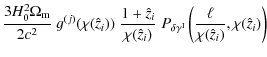
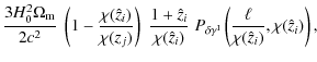
where the approximation has been applied to distribution i in the first step and to distribution j in the second equality. The latter transformation only affects the lensing efficiency and is readily seen by inserting the approximated distance distribution into (4). Note that the second term in (6), containing
For the sake of a compact notation we define the vectors
![$\displaystyle \frac{\mbox{\boldmath$T'$ }^{(i)}_{[0]}}{\vert\mbox{\boldmath$T'$...
... {{T'}_{[0]}^{(i)}}_j = \left( 1 - \frac{\chi(\hat{z}_i)}{\chi(z_j)} \right)\;;$](/articles/aa/full_html/2009/43/aa12420-09/img119.png)
![$\displaystyle \frac{\mbox{\boldmath$T'$ }^{(i)}_{[1]}}{\vert\mbox{\boldmath$T'$...
...box{with}~~~ {{T'}_{[1]}^{(i)}}_j = B^{(i)}(\chi(z_j)) ~\chi'(z_j) ~\Delta z_j,$](/articles/aa/full_html/2009/43/aa12420-09/img121.png)
so that the constraint (16) turns into an orthogonality relation,
![\begin{displaymath}
\Pi^{(i)}_{[q]}(\ell) = \sum_{j=i+1}^{N_z} {{T'}_{[q]}^{(i)}}_j ~P_{\rm tot}^{(ij)}(\ell),
\end{displaymath}](/articles/aa/full_html/2009/43/aa12420-09/img125.png)
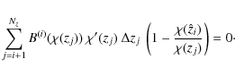
where the weights are specified by the requirement
![\begin{displaymath}
\left( \mbox{\boldmath$T$ }^{(i)}_{[q]} \cdot \mbox{\boldmat...
...^{(i)}_{[r]} \right) = 0 ~~~\mbox{for all}~~~ 0 \leq r < q\;.
\end{displaymath}](/articles/aa/full_html/2009/43/aa12420-09/img126.png)
In the discretized version given by (16) the weight function has Nz-i free parameters, namely the function values
By defining vectors that contain the cosmic shear observables,
i.e. in our case the power spectra,
and composing the transformation matrix
![\begin{displaymath}
\mbox{\boldmath$T$ }^{(i)} \equiv \left( \mbox{\boldmath$T$ ...
...)}_{[0]}, ... ,\mbox{\boldmath$T$ }^{(i)}_{[N_z-i-1]} \right)
\end{displaymath}](/articles/aa/full_html/2009/43/aa12420-09/img132.png)
for every distribution i and angular frequency
Performing a rotation, the dimension of the nulled data
vector, which is composed of the ![]() for every i and
for every i and ![]() ,
is exactly the same as for the original data set. For the data analysis
one removes the contaminated nulled power spectra with subscript
,
is exactly the same as for the original data set. For the data analysis
one removes the contaminated nulled power spectra with subscript
![]() ,
i.e. one entry per initial bin. This is the step that actually does the
nulling and modifies both statistical and systematic error budgets. In
this work, we are going to use all remaining nulled power spectra with
,
i.e. one entry per initial bin. This is the step that actually does the
nulling and modifies both statistical and systematic error budgets. In
this work, we are going to use all remaining nulled power spectra with ![]() throughout. Since they are merely specified by being composed of
mutually orthogonal weights, there is no ordering among different q.
In particular, it is impossible to make a priori statements about the
information content of different orders q.
throughout. Since they are merely specified by being composed of
mutually orthogonal weights, there is no ordering among different q.
In particular, it is impossible to make a priori statements about the
information content of different orders q.
It should be noted, however, that one can combine the
formalism
outlined above with a data compression algorithm, based on Fisher
information. As investigated in JS08, nearly all information about
cosmological parameters can be concentrated in a limited set of nulled
power spectra, constructed from the first-order weights
![]() .
The additional requirement that a suitable combination of Fisher matrix
elements is to be maximized introduces a strong hierarchy in terms of
information content into the sequence of
.
The additional requirement that a suitable combination of Fisher matrix
elements is to be maximized introduces a strong hierarchy in terms of
information content into the sequence of
![]() with
with ![]() .
We will not consider such an optimization in this work.
.
We will not consider such an optimization in this work.
2.2 Fisher matrix formalism
In the following analysis we will make use of the Fisher matrix
formalism (see Tegmark
et al. 1997
for details) to obtain parameter constraints. Probing the likelihood
locally around its maximum, it is computationally much cheaper than a
full likelihood analysis and thus useful for error estimates for a
large set of models. The elements of the Fisher matrix are defined by
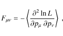
for a set of parameters
To second-order Taylor expansion around the maximum likelihood
point
the likelihood can be described by a multivariate Gaussian, so that, as
long as only regions in parameter space are probed where the
non-Gaussian contributions are negligible, it is sufficient to consider
a Gaussian likelihood
![$\displaystyle \times\; \exp \left\{ -\frac{1}{2} \left[ \mbox{\boldmath$x$ }-\m...
...boldmath$x$ }-\mbox{\boldmath$\bar{x}$ }(\mbox{\boldmath$p$ }) \right] \right\}$](/articles/aa/full_html/2009/43/aa12420-09/img143.png)
for a data vector
where the argument of
Now consider an invertible linear transformation ![]() of the data vector,
of the data vector,
In this work,
However, in the case of nulling the transformation (19) to the
new data vector ![]() depends on the cosmological parameters one aims at determining because
the elements of
depends on the cosmological parameters one aims at determining because
the elements of ![]() are composed of comoving distances. Hence, the likelihood is now
parameter-dependent in both arguments,
are composed of comoving distances. Hence, the likelihood is now
parameter-dependent in both arguments,
where we omitted the modulus of
We intend to compute the Fisher matrix for the original and
the
transformed data set, in both cases at the point of maximum likelihood,
i.e. for the fiducial set of parameters. At this point in parameter
space we expect the derivative with respect to parameters to vanish on
average,
![]() .
If the relation holds for
.
If the relation holds for ![]() ,
it is clear from (27)
that this is generally not the case for
,
it is clear from (27)
that this is generally not the case for ![]() .
Therefore we set the requirement that
.
Therefore we set the requirement that ![]() ,
which is fulfilled by the orthogonal transformation constructed in the
foregoing section. Then one can show that the Fisher matrices of both
data vectors are equivalent, even for a parameter-dependent data
transformation, as is detailed in Appendix A.
,
which is fulfilled by the orthogonal transformation constructed in the
foregoing section. Then one can show that the Fisher matrices of both
data vectors are equivalent, even for a parameter-dependent data
transformation, as is detailed in Appendix A.
Furthermore, we assume that the original covariance Cx
does not depend on cosmological parameters. Since an additional
cosmology dependence would lead to tighter constraints, this is a
conservative assumption (see e.g. Eifler et al.
2009).
Using the equivalence of the Fisher matrices, and returning to the
notation in the context of the nulling technique, we then arrive
from (25)
at the following expression for the original (index ``orig'') and the
nulled (index ``null'') data vector (see Appendix. A),

where
Since the inverse Fisher matrix is an estimate for the parameter
covariance matrix, we compute the marginalized statistical errors as
![]() .
Due to the Cramér-Rao inequality this is a lower bound on the error. To
assess the effect of the systematic, we also calculate the bias on
every parameter by means of the bias formalism (Huterer
et al. 2006; Kim
et al. 2004; Kitching
et al. 2009; Taylor
et al. 2007; Huterer
& Takada 2005; Amara
& Refregier 2008). Assuming a systematic
.
Due to the Cramér-Rao inequality this is a lower bound on the error. To
assess the effect of the systematic, we also calculate the bias on
every parameter by means of the bias formalism (Huterer
et al. 2006; Kim
et al. 2004; Kitching
et al. 2009; Taylor
et al. 2007; Huterer
& Takada 2005; Amara
& Refregier 2008). Assuming a systematic ![]() that is subdominant with respect to the signal and causes only small
systematic errors, the bias b on a parameter
that is subdominant with respect to the signal and causes only small
systematic errors, the bias b on a parameter ![]() can be calculated by
can be calculated by
and likewise for the nulled data set. A formal derivation of the bias formalism, including the discussion of its limitations can be found in Appendix B.
3 Modeling
3.1 Redshift distributions
To model realistic redshift probability distributions of
galaxies in
the presence of photometric redshift errors, we keep close to the
formalisms used in Ma et al. (2006)
and Amara &
Refregier (2007).
We assume survey parameters that should be representative of any future
space-based mission aimed at precision measurements of cosmic shear,
such as the Euclid satellite proposed to ESA. Note that the probability
distributions of comoving distances and redshift, used in parallel in
this work, are related via
![]() .
.
According to Smail et al.
(1994) we assume an overall redshift probability distribution
with
where the zi mark the redshifts of the bin boundaries, and where z0=0 and
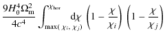
![\begin{figure}
\par\includegraphics[scale=.6]{12420fg1.ps}\end{figure}](/articles/aa/full_html/2009/43/aa12420-09/img183.png)
|
Figure 1:
Number density distribution of galaxies for a division into Nz=5
redshift bins, rendered dimensionless through dividing by the total
number density n.
The thick solid line corresponds to the overall galaxy number density
distribution, normalized to unity. The thin curves represent the
distributions corresponding to the five photometric redshift bins,
normalized to 1/Nz.
The original bin boundaries are chosen according to (31).
Note that the sum of the individual distributions adds up to the total
distribution for every z. Top panel:
resulting distributions for |
| Open with DEXTER | |
Our model for photometric redshift errors accounts for two
effects,
a statistical uncertainty characterized by the redshift dispersion
![]() ,
and misidentifications of a fraction
,
and misidentifications of a fraction ![]() of galaxies with offsets from the center of the distribution of
of galaxies with offsets from the center of the distribution of ![]()
![]() .
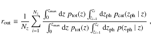
We write the conditional probability of obtaining a photometric
redshift
.
We write the conditional probability of obtaining a photometric
redshift ![]() given the true, spectroscopic redshift z as
given the true, spectroscopic redshift z as

where
Due to the multiplication by
The number density of galaxies located in photometric redshift
bin i as a function of spectroscopic redshift is
given by

so that evidently
Two examples for galaxy distributions n(i)(z)
obtained via this formalism are shown in Fig. 1,
one without outliers and with a dispersion of ![]() ,
and one where outliers with
,
and one where outliers with ![]() at an offset
at an offset ![]() have been added. As is evident from the plot in the lower panel, the
outlier Gaussians are modified by (33) into
elongated bumps, which are well separated from the central peak. They
are most prominent as a distribution with
have been added. As is evident from the plot in the lower panel, the
outlier Gaussians are modified by (33) into
elongated bumps, which are well separated from the central peak. They
are most prominent as a distribution with ![]() ,
being part of the lowest photometric bin, and a broad distribution at
low redshifts, belonging to the highest photometric bin. This behavior
is qualitatively in good agreement with the characteristic shape of the
scatter plots in the spectroscopic redshift - photometric redshift
plane, as for instance analyzed in Abdalla
et al. (2007), which also justifies our choice of
,
being part of the lowest photometric bin, and a broad distribution at
low redshifts, belonging to the highest photometric bin. This behavior
is qualitatively in good agreement with the characteristic shape of the
scatter plots in the spectroscopic redshift - photometric redshift
plane, as for instance analyzed in Abdalla
et al. (2007), which also justifies our choice of ![]() .
.
![\begin{figure}
\par\includegraphics[scale=.6,angle=270]{12420fg2.ps}
\end{figure}](/articles/aa/full_html/2009/43/aa12420-09/img204.png)
|
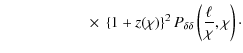
Figure 2:
Relation between |
| Open with DEXTER | |
To judge the performance of nulling in the presence of
catastrophic
outliers in the redshift distributions, it is important to note that
![]() does not equal the true fraction of outliers, primarily because of the
subsequent multiplication of (32)
by the overall redshift distribution
does not equal the true fraction of outliers, primarily because of the
subsequent multiplication of (32)
by the overall redshift distribution ![]() ,
see (33).
We compute the true fraction of outliers, denoted by
,
see (33).
We compute the true fraction of outliers, denoted by ![]() ,
as the part of a redshift distribution that is contained in the two
outlier Gaussians of our model. A quantity
,
as the part of a redshift distribution that is contained in the two
outlier Gaussians of our model. A quantity ![]() is defined identically to (32),
but with the first term, i.e. the central Gaussian, removed. Then we
define the outlier fraction as
is defined identically to (32),
but with the first term, i.e. the central Gaussian, removed. Then we
define the outlier fraction as
where
In Fig. 2 the
relation between ![]() and
and ![]() for fixed
for fixed ![]() is plotted. The gray region comprises the results for the range from
is plotted. The gray region comprises the results for the range from ![]() to
to ![]() .
Evidently, the true fraction of outliers is smaller than
.
Evidently, the true fraction of outliers is smaller than ![]() ,
reaching up to about
,
reaching up to about ![]() for
for ![]() .
The strongest contribution to
.
The strongest contribution to
![]() originates
from the bins at the lowest and highest redshifts, where the outlier
distributions are enhanced because one of the outlier Gaussians is
located in a redshift regime where
originates
from the bins at the lowest and highest redshifts, where the outlier
distributions are enhanced because one of the outlier Gaussians is
located in a redshift regime where
![]() obtains high values. The redshift distributions centered at medium
redshifts have their central Gaussian at
obtains high values. The redshift distributions centered at medium
redshifts have their central Gaussian at ![]() where
where ![]() peaks, so that the outlier fraction in the corresponding bins is small.
peaks, so that the outlier fraction in the corresponding bins is small.
In the following, we will consider the range ![]() ,
which yields outlier fractions that should comprise realistic limits of
catastrophic failures in the photometric redshift determination of
surveys aimed at measuring cosmic shear tomography (see Abdalla
et al. 2007). For the COSMOS field Ilbert et al.
(2009) found photometric redshift dispersions in the range
between 0.007 for the brightest galaxies and 0.06 for fainter objects
up
,
which yields outlier fractions that should comprise realistic limits of
catastrophic failures in the photometric redshift determination of
surveys aimed at measuring cosmic shear tomography (see Abdalla
et al. 2007). For the COSMOS field Ilbert et al.
(2009) found photometric redshift dispersions in the range
between 0.007 for the brightest galaxies and 0.06 for fainter objects
up ![]() .
Taking these values as a reference, we are going to consider the range
.
Taking these values as a reference, we are going to consider the range ![]() .
.
3.2 Lensing power spectra
As the basis for our analysis we use sets of tomography lensing power
spectra which are computed for a ![]() CDM universe with fiducial
parameters
CDM universe with fiducial
parameters ![]() ,
,
![]() ,
and
,
and ![]() with h100
= 0.7. Throughout, the spatial geometry of the
Universe is assumed to be flat. We incorporate a variable dark energy
scenario by parametrizing its equation of state, relating pressure
with h100
= 0.7. Throughout, the spatial geometry of the
Universe is assumed to be flat. We incorporate a variable dark energy
scenario by parametrizing its equation of state, relating pressure
![]() to density
to density ![]() ,
as
,
as

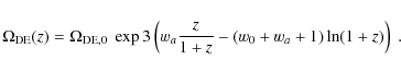
where the cosmological constant is chosen as the fiducial model, i.e. w0=-1 and wa=0. Then the dark energy density parameter reads
The three-dimensional power spectrum of matter density fluctuations
![\begin{figure}
\par\includegraphics[scale=.77,angle=270]{12420fg3.ps}
\end{figure}](/articles/aa/full_html/2009/43/aa12420-09/img228.png)
|
Figure 3:
Original and nulled tomography power spectra as a function of angular
frequency. The survey has been divided into Nz=10
photometric redshift bins with dispersion 0.03(1+z).
Top right panels: lensing power spectra |
| Open with DEXTER | |
The nulled power spectra ![]() are then calculated via (19). The
nulling weights
are then calculated via (19). The
nulling weights ![]() ,
see (18),
are computed for the fiducial cosmology, while the higher orders are
obtained by Gram-Schmidt ortho-normalization. The Gram-Schmidt
procedure does not uniquely define the order of the orthogonal vectors,
so that no particular ordering is assigned to q, as
opposed to the approach in JS08, where a higher order q
corresponded to a lower information content in
,
see (18),
are computed for the fiducial cosmology, while the higher orders are
obtained by Gram-Schmidt ortho-normalization. The Gram-Schmidt
procedure does not uniquely define the order of the orthogonal vectors,
so that no particular ordering is assigned to q, as
opposed to the approach in JS08, where a higher order q
corresponded to a lower information content in ![]() .
.
On applying nulling to a real data set, one has to assume the values of
the relevant parameters ![]() ,
,
![]() ,
w0, and wa
to obtain
,
w0, and wa
to obtain ![]() .
Whilst it is a realistic premise that these parameters are
approximately known, slightly incorrect assumptions may degrade the
downweighting of the GI signal, but do not introduce a new bias to the
parameter estimation, as will be assessed in detail in Sect. 4.2. A
sample of both original and nulled tomography power spectra are plotted
in Fig. 3.
For this sample the nulling has been performed following variant (C),
which will be discussed in detail in Sect. 4.1.
.
Whilst it is a realistic premise that these parameters are
approximately known, slightly incorrect assumptions may degrade the
downweighting of the GI signal, but do not introduce a new bias to the
parameter estimation, as will be assessed in detail in Sect. 4.2. A
sample of both original and nulled tomography power spectra are plotted
in Fig. 3.
For this sample the nulling has been performed following variant (C),
which will be discussed in detail in Sect. 4.1.
As regards the calculation of the power spectrum covariance (Joachimi
et al. 2008,
and references therein), entering the Fisher matrix, we have to specify
further survey characteristics in addition to the aforementioned
redshift probability distribution. We assume a survey size of
![]() and a total number density of galaxies of
and a total number density of galaxies of ![]() ,
resulting in approximately
,
resulting in approximately ![]() galaxies per photometric redshift bin. To compute shot noise, the
dispersion of intrinsic ellipticities is set to
galaxies per photometric redshift bin. To compute shot noise, the
dispersion of intrinsic ellipticities is set to ![]() .
These survey parameters correspond to those representative of future
cosmic shear satellite missions such as Euclid.
.
These survey parameters correspond to those representative of future
cosmic shear satellite missions such as Euclid.
3.3 Intrinsic alignment signal
To quantify the bias on cosmological parameters before and
after
nulling, a GI systematic power spectrum is added to the data vector. We
adopt the ``non-linear linear alignment model'' of Bridle & King
(2007), who suggest to compute the three-dimensional
matter-intrinsic shear cross-power spectrum as
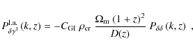
where
Originating from analytical considerations by HS04, the linear alignment model in the form employed here lacks solid physical motivation, but fits within the error bars of Mandelbaum et al. (2006). It also provides reasonable fits to the results of the halo model considerations by Schneider & Bridle (2009).
While the nulling technique as such is completely independent
of the
actual functional form of the systematic, the residual bias does depend
on the GI signal. Thus, we consider an additional set of simplistic
power-law GI power spectra for reference. They are
given by
where
The resulting power spectra are also shown in Fig. 3. As already
mentioned in Bridle
& King (2007),
the linear alignment model produces a strong systematic, partially
surpassing the lensing signal in amplitude for cross-correlations of
largely different redshift bins. Since the GI term is negative, the sum
of lensing and intrinsic alignment power spectrum can become negative
in the corresponding ![]() -range
in these cases
-range
in these cases![]() .
Due to our choice of normalization, the power-law toy GI signal can
dominate the lensing power spectrum on even larger angular frequency
intervals.
.
Due to our choice of normalization, the power-law toy GI signal can
dominate the lensing power spectrum on even larger angular frequency
intervals.
After nulling, the systematic is largely suppressed, oscillating around zero for the lower redshift bins. Still, significant residual signals remain because the finite extent of the redshift probability distributions has been neglected in the derivation of nulling. In particular, the systematic signal is eliminated only at a single redshift within each bin, thus being merely downweighted in neighboring redshift ranges. A detailed discussion about the sources of the residual bias will follow in Sect. 5. We note that nulling works independently of the strength of the systematic; it can even be applied to data in which the GI term surpasses the cosmic shear signal.
We have also added II power spectra to Fig. 3 in order to judge in how far our assumption of dropping the II signal in our considerations is valid. The original II power spectra yield a strong contribution for auto-correlations, but drop off quickly if the correlated redshift distributions have less overlap. In the transformed data set, the II contamination is smaller than the residual GI signal and thus negligible for power spectra with q > 1. For q=1 however, the II signal is significant such that in this case nulling would have to be preceded by an II removal technique. In the limit of completely disjoint photometric bins, the II signal would be confined to auto-correlations in the original data set. Since these are not included into the construction of the nulled power spectra, the latter would be completely free of II terms in this idealized case.
Table 1: Upper limits on the allowed angular frequency range if the II contamination in the nulled data shall be suppressed by at least a factor of s with respect to the nulled GG term.
To ensure that the II term remains sufficiently small compared
to
the GG signal, one could restrict the subsequent analysis partly to
larger angular scales. For instance, to achieve a minimum suppression
by a factor s of the II signal with respect to the
lensing signal, we determine maximum allowed ![]() -values, given in
Table 1.
These upper bounds would only have to be applied to orders q=1,
and are valid in the case of the setup used to produce Fig. 3.
The limitations due to the II contamination are expected to become more
restrictive as the photometric redshift scatter increases.
-values, given in
Table 1.
These upper bounds would only have to be applied to orders q=1,
and are valid in the case of the setup used to produce Fig. 3.
The limitations due to the II contamination are expected to become more
restrictive as the photometric redshift scatter increases.
Alternatively, our findings suggest that, due to the
confinement of
the II term to a limited set of nulled power spectra, a treatment of
the II signal after nulling may also
provide a promising ansatz. In the current implementation the nulled
power spectra of order q=1 have a dominating
contribution from original power spectra ![]() with j=i+1,
which contain the bulk of the II signal after the removal of
auto-correlations from the analysis. Hence, the residual II terms
accumulate within the measures of order q=1. The
freedom to choose the weights of (19) in the
subspace orthogonal to
with j=i+1,
which contain the bulk of the II signal after the removal of
auto-correlations from the analysis. Hence, the residual II terms
accumulate within the measures of order q=1. The
freedom to choose the weights of (19) in the
subspace orthogonal to ![]() allows for a more specific treatment of the II signal in the nulled
data. We emphasize that the final goal is a simultaneous removal of all
intrinsic alignment contributions, but this is beyond the scope of this
paper and subject to future work.
allows for a more specific treatment of the II signal in the nulled
data. We emphasize that the final goal is a simultaneous removal of all
intrinsic alignment contributions, but this is beyond the scope of this
paper and subject to future work.
As the GI contamination has a large amplitude, the question is raised
whether the bias formalism, i.e. (29), still
yields accurate results. The effect of a large systematic is
investigated in detail in Appendix B.
We conclude from our findings that even for a strong GI term the bias
is obtained with good accuracy whereas the statistical errors, which
are also affected by a strong systematic, can deviate more
significantly. To guarantee results that are as close as possible to a
full likelihood analysis, we downscale all GI signals by a factor of
five throughout the subsequent sections. Since the bias is proportional
to the overall amplitude of the systematic, and since we are mostly
going to consider ratios of biases, the rescaling does not have an
influence on the statements concerning the performance of nulling.
Merely the mean square error, defined by
is affected because the systematic error becomes less dominant. A lower systematic amplitude slightly disfavors nulling as it lowers the bias while causing an increase in statistical errors. Besides, limiting the strength of biases avoids unphysical parameter estimates as for instance
In surveys with a significant GI systematic, intrinsic ellipticity correlations are likely to affect parameter estimation, too. To restrict our considerations to the GI contamination, we follow Takada & White (2004), excluding auto-correlations from both original and nulled data vectors, and assuming that the remaining measures do not have an II signal. Note that due to the exclusion of auto-correlation power spectra the statistical errors on cosmological parameters in this work are larger than those of other cosmic shear tomography analyses, even for our original data sets.
Excluding auto-correlations is of limited accuracy to control the II signal since we use a relatively dense binning, partially with large photometric errors, so that cross-correlations of adjacent photometric redshift bins would contain significant II terms as well. With realistic data one could in principle let the nulling be preceded by an II removal technique such as King & Schneider (2002) who also take a purely geometric approach. However, the redshift-dependent weighting of galaxy pairs, on which the II removal is based, modifies the calculation of the projected cosmic shear measures such as (2), which in turn entails a modification of the nulling weights. The improvements of the nulling technique we investigate in Sect. 5.3 will also constitute an efficient tool to control the II term.
4 Improving the nulling performance
4.1 Optimizing the nulling weights
In the composition of the nulling weights (18) one has
the freedom to choose the specific redshift ![]() within the initial bin at which the GI contribution is eliminated, as
well as the referencing of redshifts zj
to the background redshift bins. For convenience JS08 placed
within the initial bin at which the GI contribution is eliminated, as
well as the referencing of redshifts zj
to the background redshift bins. For convenience JS08 placed ![]() at the center of the initial bin and identified zj
with the lower boundary of bin j.
Since this choice was fairly arbitrary, we seek to find a more
appropriate referencing that leads to a minimum residual GI
contamination.
at the center of the initial bin and identified zj
with the lower boundary of bin j.
Since this choice was fairly arbitrary, we seek to find a more
appropriate referencing that leads to a minimum residual GI
contamination.
![\begin{figure}
\par\includegraphics[scale=.45,clip]{12420fg4.ps}\includegraphics[scale=.45,clip]{12420fg5.ps}
\end{figure}](/articles/aa/full_html/2009/43/aa12420-09/img248.png)
|
Figure 4:
Comparison of the performance of the different nulling weights. Shown
are marginalized statistical errors |
| Open with DEXTER | |
A more natural choice is to position both the redshift of the initial
bin ![]() and the reference redshifts of the background bins at the center
between the photometric redshift bin boundaries, denoted by
and the reference redshifts of the background bins at the center
between the photometric redshift bin boundaries, denoted by ![]() .
This setup does not require knowledge about the redshift probability
distribution of each bin, although this information has to be available
at high precision for future cosmic shear surveys. Hence, we
furthermore define nulling weights that take redshift information into
account. Re-examining (17),
one can drop the approximation of narrow redshift/distance probability
distributions for the background bins, keeping the first equality
of (17).
Thereby, instead of the comoving distance ratio
.
This setup does not require knowledge about the redshift probability
distribution of each bin, although this information has to be available
at high precision for future cosmic shear surveys. Hence, we
furthermore define nulling weights that take redshift information into
account. Re-examining (17),
one can drop the approximation of narrow redshift/distance probability
distributions for the background bins, keeping the first equality
of (17).
Thereby, instead of the comoving distance ratio ![]() ,
one directly uses the lensing efficiency, which is the average of this
ratio, weighted by the redshift/distance probability distribution of
the background photometric redshift bin. The zeroth-order nulling
weight in (18)
is then given by
,
one directly uses the lensing efficiency, which is the average of this
ratio, weighted by the redshift/distance probability distribution of
the background photometric redshift bin. The zeroth-order nulling
weight in (18)
is then given by ![]() .
For the remaining free redshift of the initial bin
.
For the remaining free redshift of the initial bin ![]() we choose the median redshift of distribution i, a
measure that contains information about the form of the distribution,
but is robust against outliers.
we choose the median redshift of distribution i, a
measure that contains information about the form of the distribution,
but is robust against outliers.
Table 2: Overview on nulling variants considered.
Hence, in total we are going to consider three different
versions of
nulling: (A) the ``old'' version of nulling with referencing to the
lower boundaries of the background bins, a variant (B) where the
background bins are identified with the bin centers
![]() instead, and (C) the nulling that includes detailed redshift
information via assigning the foreground bins to their median redshifts
and using the comoving distance ratio, weighted by
instead, and (C) the nulling that includes detailed redshift
information via assigning the foreground bins to their median redshifts
and using the comoving distance ratio, weighted by
![]() ,
as the zeroth-order nulling weight. The properties of these variants
are summarized in Table 2.
,
as the zeroth-order nulling weight. The properties of these variants
are summarized in Table 2.
In Fig. 4
the performance of nulling with different nulling weights is shown. We
plot the marginalized statistical error ![]() and the relative bias
and the relative bias
where
The left column of Fig. 4
illustrates the change in errors due to nulling with the referencing
used hitherto, i.e. variant (A). While the marginalized statistical
errors increase by up to a factor of about three for the weakly
constrained dark energy parameters, the bias drops from values of up to
![]() to numbers
that are of the same order of magnitude as the original statistical
errors, i.e.
to numbers
that are of the same order of magnitude as the original statistical
errors, i.e. ![]() .
For parameters that were strongly biased this leads to a considerable
decrease in the mean square error, but
.
For parameters that were strongly biased this leads to a considerable
decrease in the mean square error, but ![]() may also slightly increase if the systematic was subdominant already
before nulling as is the case for the Hubble parameter.
may also slightly increase if the systematic was subdominant already
before nulling as is the case for the Hubble parameter.
In the right column of Fig. 4 resulting errors for all three nulling variants are given. It is evident that the newly introduced versions (B) and (C) of nulling perform significantly better in removing the systematic. Variant (B) decreases the bias by at least a factor of three with respect to (A), reversing the sign of the bias for almost all parameters. This hints at using the reference redshifts of the nulling weights as free parameters to control the amount of bias allowed in the data, as will be further discussed in Sect. 8. Variant (C) nearly perfectly eliminates the GI contamination. Although the underlying data lacks photometric redshift errors, knowledge about the distributions p(i)(z) is still advantageous as e.g. the lowest and highest redshift bin are broad and largely asymmetric. Regarding statistical errors, the better a version is capable of removing the systematic, the less stringent parameter constraints become. However, the improved bias reduction clearly outweighs the marginal increase in statistical errors.
In summary, we propose to henceforth use nulling with referencing to the centers of photometric redshift bin divisions, i.e. variant (B), in absence of detailed information about redshift distributions, and else version (C) which exploits this knowledge. Both approaches will be considered in the following analyses.
4.2 Cosmology-dependence of the nulling weights
The nulling weights T[q](i)j
depend on those parameters of the cosmological model that enter the
comoving distance in a non-trivial way, i.e. for our model assumptions
![]() ,
w0, and wa.
Since only ratios of comoving distances enter the nulling weights,
there is no dependence on h100
which enters the prefactor of (3).
If the relevant cosmological parameters chosen to compute the nulling
weights are different from the true parameters of the data set, the
performance of nulling may deteriorate. A grossly incorrect choice of
nulling weights could in principle affect the lensing signal more than
the GI term, which could then even cause a larger bias on parameters in
the transformed data than in the original one.
,
w0, and wa.
Since only ratios of comoving distances enter the nulling weights,
there is no dependence on h100
which enters the prefactor of (3).
If the relevant cosmological parameters chosen to compute the nulling
weights are different from the true parameters of the data set, the
performance of nulling may deteriorate. A grossly incorrect choice of
nulling weights could in principle affect the lensing signal more than
the GI term, which could then even cause a larger bias on parameters in
the transformed data than in the original one.
![\begin{figure}
\par\includegraphics[scale=.46]{12420fg6.ps}
\end{figure}](/articles/aa/full_html/2009/43/aa12420-09/img262.png)
|
Figure 5: Cosmology
dependence of the nulling weights. The change in estimates for the
cosmological parameters, entering the distance-redshift relation
non-trivially, is plotted for different iteration steps. The estimates
resulting from using variant (C) are shown as solid lines, those for
variant (B) as dashed lines. Iteration 0 corresponds to the
initial values for the parameters, in this case the results of the
analysis of the unmodified data set. For reference, the estimates
obtained by using the true underlying cosmology to compute the nulling
weights are plotted as thin lines. The hatched regions around these
lines signify the 1 |
| Open with DEXTER | |
Avoiding any a priori guesses of the true values of the
relevant
cosmological parameters, we explore the cosmology dependence of the
nulling weights by taking the estimates from the analysis of the
original data set as input cosmology for the computation of the
T[q](i)j.
As we use the linear alignment model (38),
the estimates ![]() ,
where
,
where ![]() is the true parameter value and b
is the bias, are far from the true values and beyond any decent a
priori guess, so that this setup can be understood as a worst-case
scenario. With the weights obtained this way, the nulled data can be
analyzed, yielding another set of parameter estimates. This can then be
taken as input for a refined set of nulling weights, thereby creating
an iterative process which can be terminated when successive iterations
yield stable parameter estimates.
is the true parameter value and b
is the bias, are far from the true values and beyond any decent a
priori guess, so that this setup can be understood as a worst-case
scenario. With the weights obtained this way, the nulled data can be
analyzed, yielding another set of parameter estimates. This can then be
taken as input for a refined set of nulling weights, thereby creating
an iterative process which can be terminated when successive iterations
yield stable parameter estimates.
In Fig. 5 the results of this iteration process are shown for nulling variants (B) and (C), both showing a very similar behavior. The parameter estimates for iteration 0 correspond to the estimates of the analysis of the original data set. Given these largely incorrect input parameters, nulling is still able to reduce the bias due to intrinsic alignment to a level close to the one when using the true cosmology as input. Already after the first iteration step the residual bias is considerably smaller than the statistical errors. After at most two iterations, the results for the residual bias are indistinguishable from those with the correct input parameters.
Hence, the dependence of the nulling weights on cosmology is only weak, being solely due to geometrical terms. Consequently, nulling is robust against an incorrect initial guess for cosmological parameters needed to compute the nulling weights. For a consistency check, the iterative procedure outlined above can be performed on the data. In the remainder of this work we will use the true cosmology to calculate the nulling weights for reasons of simplicity.
5 Influence of redshift information on nulling
5.1 Redshift binning
First, we investigate the performance of nulling as a function
of
the number of photometric redshift bins the survey is divided into. The
larger Nz,
the better (16)
is an approximation of (13),
so that the GI removal is expected to work more efficiently.
Furthermore, since nulling eliminates the contribution to the lensing
signal of the background objects only at a single redshift, more
concentrated redshift probability distributions are nulled more
accurately, given an appropriately chosen redshift ![]() within the initial bin. At the same time, less statistical information
is lost because the entries of the transformed data vector, which are
removed in the process of nulling, contain less independent information
if the redshift distributions have a smaller spacing.
within the initial bin. At the same time, less statistical information
is lost because the entries of the transformed data vector, which are
removed in the process of nulling, contain less independent information
if the redshift distributions have a smaller spacing.
In search for a single quantity that measures an overall power
of a
data set to constrain cosmological parameters we define the average
statistical power as
where
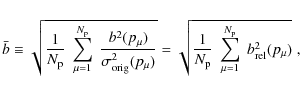
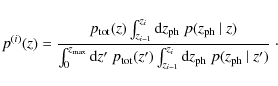
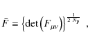
which is the root mean square of the ratio of the systematic over the statistical error before nulling over all considered parameters. We refer to the performance of nulling via the ratios
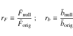
of
![\begin{figure}
\par\includegraphics[scale=.61,angle=270]{12420fg7.ps}
\end{figure}](/articles/aa/full_html/2009/43/aa12420-09/img272.png)
|
Figure 6:
Ratios rF
and rb as
a function of the number of photometric redshift bins Nz.
Thin curves represent rF,
thick curves rb.
Results for zero photometric redshift error are given as solid black
lines; results for |
| Open with DEXTER | |
Figure 6
shows results for the ratios rF
and rb
for different Nz,
both without photometric redshift errors and for ![]() .
In this section the linear alignment model is used as the systematic,
downscaled by a factor of five. For five redshift bins
.
In this section the linear alignment model is used as the systematic,
downscaled by a factor of five. For five redshift bins ![]() is only about a third of
is only about a third of ![]() ,
but rF
rises, first strongly and then with an increasingly shallow slope for
larger Nz.
This development is mostly based on the improving performance of
nulling since for a cosmic shear tomography data set statistical errors
only marginally decrease for
,
but rF
rises, first strongly and then with an increasingly shallow slope for
larger Nz.
This development is mostly based on the improving performance of
nulling since for a cosmic shear tomography data set statistical errors
only marginally decrease for ![]() (see e.g. Ma et al. 2006;
Hu 1999; Bridle
& King 2007; Simon
et al. 2004; JS08).
(see e.g. Ma et al. 2006;
Hu 1999; Bridle
& King 2007; Simon
et al. 2004; JS08).
Introducing a photometric redshift dispersion of ![]() ,
one finds that, for small Nz,
rF
increases in the same way as in the case without photometric redshift
errors. As soon as the size of the redshift bins attains the same order
as the width of the dispersion
,
one finds that, for small Nz,
rF
increases in the same way as in the case without photometric redshift
errors. As soon as the size of the redshift bins attains the same order
as the width of the dispersion
![]() ,
less additional redshift information becomes available to constrain
parameters. Since nulling, like other techniques that deal with the
control of intrinsic alignments (e.g. Bridle & King
2007), requires more precise redshift information, the curve
for rF
levels off.
,
less additional redshift information becomes available to constrain
parameters. Since nulling, like other techniques that deal with the
control of intrinsic alignments (e.g. Bridle & King
2007), requires more precise redshift information, the curve
for rF
levels off.
Even for only five bins in redshift, nulling is capable of reducing the
average bias ![]() by more than
by more than ![]() for perfect redshift information. For
for perfect redshift information. For ![]() ,
less than
,
less than ![]() of the average bias remains. If a more realistic photometric redshift
dispersion is present in the data, rb
significantly degrades to approximately 0.15 for Nz=5.
For ten photometric redshift bins a minimum value of
of the average bias remains. If a more realistic photometric redshift
dispersion is present in the data, rb
significantly degrades to approximately 0.15 for Nz=5.
For ten photometric redshift bins a minimum value of ![]() is
achieved before this ratio increases again for more bins, meaning that
the treatment of the systematic worsens in spite of the improvement of
redshift information due to the finer division of photometric
redshifts. This apparent contradiction requires a more thorough
investigation and will be addressed in Sect. 5.3.
is
achieved before this ratio increases again for more bins, meaning that
the treatment of the systematic worsens in spite of the improvement of
redshift information due to the finer division of photometric
redshifts. This apparent contradiction requires a more thorough
investigation and will be addressed in Sect. 5.3.
![\begin{figure}
\par\includegraphics[scale=.58,angle=270]{12420fg8.ps}
\end{figure}](/articles/aa/full_html/2009/43/aa12420-09/img280.png)
|
Figure 7: Ratio rF as a function of the number of photometric redshift bins Nz. This result has been obtained by means of a simplified Fisher matrix calculation, placing galaxies at fixed redshifts and neglecting cosmic variance in the covariance. For large Nz the increase in rF is slower than logarithmic. |
| Open with DEXTER | |
5.2 Minimum information loss
Given ideal spectroscopic redshift information, equivalent to
considering the limit ![]() ,
it would be possible to precisely eliminate the GI contamination at a
given redshift, see (17), so
that rb
tends to zero in absence of photometric redshift errors, as is indeed
the case. However, the curves for rF
in Fig. 6
apparently indicate that the full statistical information is not
regained in this limit, i.e. rF
does not tend to unity. We investigate this further by calculating rF
out to larger Nz,
assuming a simplified model with infinitesimally narrow redshift bins,
,
it would be possible to precisely eliminate the GI contamination at a
given redshift, see (17), so
that rb
tends to zero in absence of photometric redshift errors, as is indeed
the case. However, the curves for rF
in Fig. 6
apparently indicate that the full statistical information is not
regained in this limit, i.e. rF
does not tend to unity. We investigate this further by calculating rF
out to larger Nz,
assuming a simplified model with infinitesimally narrow redshift bins,
and a covariance that contains only shot noise. The resulting curve, shown in Fig. 7, increases slower than logarithmically as a function of Nz, so that one can expect that indeed nulling inevitably reduces the statistical power of a data set, even when spectroscopic redshifts would be available.
To illustrate this effect, consider again the continuous,
integral version of (18),
still in the limit of perfect redshift information. Choosing the
zeroth-order nulling weight proportional to ![]() ,
see (18),
one can write the corresponding transformed power spectrum as
,
see (18),
one can write the corresponding transformed power spectrum as


where in order to arrive at the second equality, the lensing power spectrum for spectroscopic redshifts has been obtained by inserting (46) into (2). Note that the upper limit in the integration over
Comparing (48) to (2), one finds that the term
5.3 Intrinsic alignment contamination from adjacent bins
The increase in rb
for large Nz
in the case ![]() ,
as seen in Fig. 6,
can be explained by inspecting (6).
To produce a GI effect, the intrinsic alignment has to act on the
foreground galaxy while the background galaxy is lensed. Hence, the GI
signal should stem from the first term in (6),
whereas the second term that contains
,
as seen in Fig. 6,
can be explained by inspecting (6).
To produce a GI effect, the intrinsic alignment has to act on the
foreground galaxy while the background galaxy is lensed. Hence, the GI
signal should stem from the first term in (6),
whereas the second term that contains ![]() with i<j vanishes if the
redshift probability distributions are disjoint, see (17). We
refer to the latter expression as the gp-term
hereafter. This term can yield a contribution to the systematic in case
the distributions overlap such that the true position of a galaxy from
the background population is in front of galaxies from the foreground
distribution. The contribution to the GI signal by swapped galaxy
positions is not accounted for by nulling and produces a residual
systematic.
with i<j vanishes if the
redshift probability distributions are disjoint, see (17). We
refer to the latter expression as the gp-term
hereafter. This term can yield a contribution to the systematic in case
the distributions overlap such that the true position of a galaxy from
the background population is in front of galaxies from the foreground
distribution. The contribution to the GI signal by swapped galaxy
positions is not accounted for by nulling and produces a residual
systematic.
To quantify the effect caused by the gp-term, we
compute the average bias for the same model of the three-dimensional GI
power spectrum, but now with the gp-term removed
from (6).
The resulting ratio rb
is plotted in Fig. 6 as well.
While this curve shows a similar behavior than the one for the
systematic with gp-term for ![]() ,
it does not follow the turnaround and continues to decrease for larger Nz
down to values of rb
obtained for data without photometric redshift errors, as expected.
Thus, the increase in rb
of the data with
,
it does not follow the turnaround and continues to decrease for larger Nz
down to values of rb
obtained for data without photometric redshift errors, as expected.
Thus, the increase in rb
of the data with ![]() for Nz
> 10 can indeed be explained by the contamination due to the gp-term.
for Nz
> 10 can indeed be explained by the contamination due to the gp-term.
The gp-term cannot be quantified in detail as it depends explicitly on the form of the matter-intrinsic shear power spectrum, see (6). However, it is produced by an overlap of the redshift distributions of foreground and background distributions, so that the gp-term can be controlled by removing or downweighting bin combinations with a large overlap in redshift, in particular adjacent photometric redshift bins. For instance, one can simply exclude power spectra for bins (ij) with j=i+1 from the analysis, which results in the dotted curves given in Fig. 6. Indeed the contamination by the gp-term is suppressed, producing merely a less significant increase in rb for Nz>20, but the statistical power decreases dramatically due to the removal of all power spectra with j=i+1.
To alleviate this effect, we propose to downweight adjacent redshift
bin combinations. According to (20),
increasing an entry in the zeroth-order nulling weight implies a lower
value in the corresponding entries of the higher-order weights. Hence,
a manipulation of the zeroth-order weights can be used to downweight
certain power spectra in the process of nulling. We introduce the
following modified weights
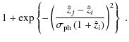
To motivate this choice, consider that for
Therefore, the wij
are expected to follow the redshift dependence of the gp-term,
so that the higher-order nulling weights ![]() with
with ![]() efficiently downweight its contribution. Note that the modification of
the nulling weights is done before normalization such that the vectors
efficiently downweight its contribution. Note that the modification of
the nulling weights is done before normalization such that the vectors
![]() still have unit length. As an aside, the weighting scheme (49)
would also contribute to the downweighting of contaminations by the II
term.
still have unit length. As an aside, the weighting scheme (49)
would also contribute to the downweighting of contaminations by the II
term.
Applying this Gaussian weighting scheme to the nulling procedure, one
obtains the gray curves of Fig. 6. While
for a small number of redshift bins rF
is similar to the case where all power spectra except auto-correlations
were used, the curve approaches the results for the case with power
spectra of adjacent bins removed for large Nz.
This means that for small Nz
the overlap between redshift bins is marginal, so that the weighting
has only little effect, whereas for many bins power spectra with j=i+1
are largely downweighted such that removing them produces similar
results. The Gaussian weighting ensures that ![]() for all Nz>10.
We will further consider the performance of this weighting scheme in
Sect. 7.1.
for all Nz>10.
We will further consider the performance of this weighting scheme in
Sect. 7.1.
The best binning in photometric redshifts in terms of nulling performance does not only depend on the number of bins Nz, but to a certain extent also on the choice of bin boundaries. The optimal positions of bin boundaries are determined by the detailed form of the relation between photometric and true, spectroscopic redshifts, which is specific to each survey and thus shall not be further assessed here.
6 Influence of photometric redshift uncertainty
6.1 Photometric redshift errors
This section deals with the dependence of nulling on the photometric
redshift dispersion ![]() ,
in absence of catastrophic outliers. The number of photometric redshift
bins is kept at Nz
= 10 for the remainder of this work, mainly for computational reasons.
Future cosmic shear surveys, relying on precise redshift information
and a large number of galaxy detections, will allow for considerably
more photometric redshift bins, which may be advantageous in terms of
nulling, see the foregoing section.
,
in absence of catastrophic outliers. The number of photometric redshift
bins is kept at Nz
= 10 for the remainder of this work, mainly for computational reasons.
Future cosmic shear surveys, relying on precise redshift information
and a large number of galaxy detections, will allow for considerably
more photometric redshift bins, which may be advantageous in terms of
nulling, see the foregoing section.
![\begin{figure}
\par\includegraphics[scale=.61]{12420fg9.ps}
\end{figure}](/articles/aa/full_html/2009/43/aa12420-09/img307.png)
|
Figure 8:
Top panel: ratios rF
and rb as
a function of photometric redshift dispersion |
| Open with DEXTER | |
In Fig. 8
rF is
plotted as a function of ![]() while in Fig. 9,
upper panel, the ratios of the marginalized statistical errors before
and after nulling are given for the parameters
while in Fig. 9,
upper panel, the ratios of the marginalized statistical errors before
and after nulling are given for the parameters ![]() and
and ![]() individually.
The curves for the other cosmological parameters vary considerably in
magnitude, but otherwise show the same characteristics as the ones
depicted. The ratio rF
decreases only very weakly with increasing
individually.
The curves for the other cosmological parameters vary considerably in
magnitude, but otherwise show the same characteristics as the ones
depicted. The ratio rF
decreases only very weakly with increasing ![]() for both nulling variants (B) and (C), taking values
between
0.44 and 0.48, because splitting the range of redshifts between 0 and 3
into 10 photometric redshift bins does not lead to a significant
degrading of redshift information, even for
for both nulling variants (B) and (C), taking values
between
0.44 and 0.48, because splitting the range of redshifts between 0 and 3
into 10 photometric redshift bins does not lead to a significant
degrading of redshift information, even for
![]() .
In contrast to this, the ratio of the marginalized errors of individual
cosmological parameters does vary with
.
In contrast to this, the ratio of the marginalized errors of individual
cosmological parameters does vary with ![]() ,
but changes are smaller than about 10%. The statistical errors of both
the original and the nulled data set increase for larger photometric
redshift errors similarly, but the error of the nulled set starts to do
so already at smaller
,
but changes are smaller than about 10%. The statistical errors of both
the original and the nulled data set increase for larger photometric
redshift errors similarly, but the error of the nulled set starts to do
so already at smaller ![]() ,
thereby producing a peak at
,
thereby producing a peak at ![]() in both curves in Fig. 9.
Marginalized errors for each of the seven considered parameters are a
factor of roughly two to three larger for the nulled data.
in both curves in Fig. 9.
Marginalized errors for each of the seven considered parameters are a
factor of roughly two to three larger for the nulled data.
![\begin{figure}
\par\includegraphics[scale=.58]{12420f10.ps}
\end{figure}](/articles/aa/full_html/2009/43/aa12420-09/img309.png)
|
Figure 9:
Performance of nulling as a function of photometric redshift dispersion
|
| Open with DEXTER | |
As is evident from Fig. 8,
lower panel, nulling using variant (C) is capable of reducing the
average bias caused by the linear alignment model by more than a factor
of 50 for ![]() .
Looking at the effect on the bias of individual parameters in
Fig. 9,
lower panel, one sees that the systematic is suppressed by more than 2
orders of magnitude for small
.
Looking at the effect on the bias of individual parameters in
Fig. 9,
lower panel, one sees that the systematic is suppressed by more than 2
orders of magnitude for small ![]() .
In spite of the strong intrinsic alignment signal, the bias is kept
subdominant up to
.
In spite of the strong intrinsic alignment signal, the bias is kept
subdominant up to ![]() .
The drop in rb
at
.
The drop in rb
at ![]() is also visible in Fig. 8
and can be traced back to a sign change in the residual bias for
several parameters, among them
is also visible in Fig. 8
and can be traced back to a sign change in the residual bias for
several parameters, among them ![]() and
and ![]() .
.
For larger redshift dispersions, rb
shows an approximately linear increase, which can only partially be
ascribed to the contamination by the gp-term as can
be concluded from comparing with the curve for the linear alignment
model without gp-term. The rise in rb
is caused by two effects that are visible in Fig. 9.
First, the strong relative bias in ![]() and
and ![]() for the original data set starts to slowly decrease for
for the original data set starts to slowly decrease for ![]() ,
predominantly because the statistical errors rise due to the degrading
information content in the line-of-sight direction. Second, the
residual bias after nulling increases as a function of
,
predominantly because the statistical errors rise due to the degrading
information content in the line-of-sight direction. Second, the
residual bias after nulling increases as a function of
![]() and starts to attain values of the same order as the statistical
errors, i.e.
and starts to attain values of the same order as the statistical
errors, i.e. ![]() ,
at just about
,
at just about ![]() .
The part of this degradation that cannot be traced back to the effect
by the gp-term
has to stem from the incorrect assessment of the redshift dependence of
the GI signal, either due to the approximations inherent to the
derivations of nulling or the suboptimal placement of the redshift at
which the signal is nulled.
.
The part of this degradation that cannot be traced back to the effect
by the gp-term
has to stem from the incorrect assessment of the redshift dependence of
the GI signal, either due to the approximations inherent to the
derivations of nulling or the suboptimal placement of the redshift at
which the signal is nulled.
Figure 8
also shows rb
for the power-law GI model with varying slopes. The behavior of rb
as a function of ![]() is in very good agreement with the results for the linear alignment
model, rb
reaching about 0.03 for
is in very good agreement with the results for the linear alignment
model, rb
reaching about 0.03 for ![]() ,
and up to
,
and up to ![]() higher values for
higher values for ![]() in
comparison with the linear alignment model. This suggests that at least
the orders of magnitude of our results as well as the general
conclusions drawn from a particular GI model used in this work can be
taken to robustly estimate the effects of a realistic GI contamination.
in
comparison with the linear alignment model. This suggests that at least
the orders of magnitude of our results as well as the general
conclusions drawn from a particular GI model used in this work can be
taken to robustly estimate the effects of a realistic GI contamination.
Moreover, Fig. 8,
upper panel, illustrates the performance of nulling using variant (B),
i.e. renouncing on information about the form of the redshift
probability distributions, and placing the redshift at which the signal
is nulled at the centers of the photometric redshift bins
![]() ,
respectively. This version of nulling is capable of retaining
marginally more information in the data, in particular for small
,
respectively. This version of nulling is capable of retaining
marginally more information in the data, in particular for small ![]() .
For high quality redshift information the reduction in bias is worse, rb
doubling approximately compared to variant (C). Again at
.
For high quality redshift information the reduction in bias is worse, rb
doubling approximately compared to variant (C). Again at ![]() ,
rb starts
to increase, but more steeply, so that for
,
rb starts
to increase, but more steeply, so that for ![]() nulling quickly becomes rather inefficient. As for variant (C), the
curves for rb
of the different GI models agree well in their functional form, but
yield largely different amplitudes. It is striking that the curve
calculated without the gp-term does not feature a
distinct increase for large
nulling quickly becomes rather inefficient. As for variant (C), the
curves for rb
of the different GI models agree well in their functional form, but
yield largely different amplitudes. It is striking that the curve
calculated without the gp-term does not feature a
distinct increase for large ![]() .
This suggests that variant (B), when combined with the weighting scheme
of Sect. 5.3,
could perform well also for larger photometric redshift errors, as we
will investigate in Sect. 7.1.
.
This suggests that variant (B), when combined with the weighting scheme
of Sect. 5.3,
could perform well also for larger photometric redshift errors, as we
will investigate in Sect. 7.1.
6.2 Analyzing optimal nulling redshifts
The construction of nulling weights allows for a certain
freedom in
the choice of redshifts, which the photometric redshift bins are
assigned to. We wish to investigate which choice of redshifts ![]() ,
i.e. those redshifts where the signal is nulled, is optimal in the
sense that the resulting zeroth-order nulling weights (18)
best reproduce the redshift dependence of the GI signal, and thus
effectively remove the systematic. The procedure to find such optimal
nulling redshifts, denoted by
,
i.e. those redshifts where the signal is nulled, is optimal in the
sense that the resulting zeroth-order nulling weights (18)
best reproduce the redshift dependence of the GI signal, and thus
effectively remove the systematic. The procedure to find such optimal
nulling redshifts, denoted by
![]() ,
is outlined in the following. We emphasize that the calculation of
,
is outlined in the following. We emphasize that the calculation of ![]() merely constitutes a diagnostic tool, inapplicable to data, since the
GI systematic has to be known exactly to do this.
merely constitutes a diagnostic tool, inapplicable to data, since the
GI systematic has to be known exactly to do this.
Judging from (17)
and the considerations in Sect. 4.1,
using the lensing efficiency ![]() as
zeroth-order nulling weight is most effective in case of precise
redshift information. In fact, in the limit of spectroscopic redshifts
as
zeroth-order nulling weight is most effective in case of precise
redshift information. In fact, in the limit of spectroscopic redshifts
![]() matches the redshift dependence of the GI signal perfectly. In the
approximation of infinitesimally narrow redshift probability
distributions for the photometric redshift bins with lower median
redshift, i.e. the initial bins, the redshifts
matches the redshift dependence of the GI signal perfectly. In the
approximation of infinitesimally narrow redshift probability
distributions for the photometric redshift bins with lower median
redshift, i.e. the initial bins, the redshifts ![]() would mark the position, at which the GI signal would be perfectly
removed. In reality, the photometric redshift bins i
have finite size as do the corresponding distributions of true
redshifts p(i)(z).
The nulling redshift
would mark the position, at which the GI signal would be perfectly
removed. In reality, the photometric redshift bins i
have finite size as do the corresponding distributions of true
redshifts p(i)(z).
The nulling redshift ![]() is not fully specified anymore and has to be chosen appropriately. One
reasonable choice is the median redshift of bin i,
which corresponds to nulling variant (C). In this section we treat the
is not fully specified anymore and has to be chosen appropriately. One
reasonable choice is the median redshift of bin i,
which corresponds to nulling variant (C). In this section we treat the ![]() as free parameters and determine an optimal value
as free parameters and determine an optimal value ![]() .
.
Hence, we aim at determining ![]() such that
such that ![]() fits
fits ![]() best since then nulling completely removes the intrinsic alignment
signal with
best since then nulling completely removes the intrinsic alignment
signal with ![]() as
zeroth-order weight. To this end, we compute the best fitting lensing
efficiency, using the least squares sum of all background bins j,
as
zeroth-order weight. To this end, we compute the best fitting lensing
efficiency, using the least squares sum of all background bins j,
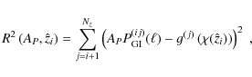
where the initial bin i and the angular frequency
Since differences in the amplitude of ![]() and
and ![]() are not of interest, the dependence of R2
on the scaling is eliminated by calculating the extremal AP
from the condition
are not of interest, the dependence of R2
on the scaling is eliminated by calculating the extremal AP
from the condition ![]() ,
yielding
,
yielding
Now R2 is computed for a wide range of
In Fig. 10
the least squares sum R2 is
plotted as a function of the ![]() for a data set with
for a data set with ![]() ,
using the downscaled linear alignment model to compute the GI power
spectrum. Note that for high redshifts
,
using the downscaled linear alignment model to compute the GI power
spectrum. Note that for high redshifts ![]() ,
the lensing efficiency tends to zero, thereby implying an extremal
value of AP=0.
Thus, the least squares go to zero for high redshifts because a GI
power spectrum, scaled to zero, fits a vanishing lensing efficiency
perfectly. The optimal nulling redshift is therefore extracted from the
well-defined local minima of R2,
which can be clearly seen in Fig. 10.
,
the lensing efficiency tends to zero, thereby implying an extremal
value of AP=0.
Thus, the least squares go to zero for high redshifts because a GI
power spectrum, scaled to zero, fits a vanishing lensing efficiency
perfectly. The optimal nulling redshift is therefore extracted from the
well-defined local minima of R2,
which can be clearly seen in Fig. 10.
![\begin{figure}
\par\includegraphics[scale=.6,angle=270]{12420f11.ps}
\end{figure}](/articles/aa/full_html/2009/43/aa12420-09/img323.png)
|
Figure 10:
Least squares sum R2 as a
function of nulling redshift |
| Open with DEXTER | |
![\begin{figure}
\par\includegraphics[scale=.6]{12420f12.ps}
\end{figure}](/articles/aa/full_html/2009/43/aa12420-09/img324.png)
|
Figure 11:
Determination of the optimal nulling redshift. Top panel:
results for |
| Open with DEXTER | |
The procedure to compute ![]() is illustrated by Fig. 11.
The redshift dependence of the GI power spectra for initial bins 1 to
3, and the corresponding best-fit lensing efficiencies are plotted,
referring the values for bin j of both quantities
to the median redshift of distribution p(j)(z)
is illustrated by Fig. 11.
The redshift dependence of the GI power spectra for initial bins 1 to
3, and the corresponding best-fit lensing efficiencies are plotted,
referring the values for bin j of both quantities
to the median redshift of distribution p(j)(z)![]() . The curves corresponding
to the lensing efficiency are obtained via linear interpolation of the
set of
. The curves corresponding
to the lensing efficiency are obtained via linear interpolation of the
set of ![]() with j=i+1, .. ,Nz.
For the
case without photometric redshift errors, nulling redshifts can be
found such that the resulting lensing efficiencies almost exactly fit
the redshift dependence of the GI power spectrum, so that in this case
the approximation of infinitesimally narrow initial bins has little
negative influence on the nulling performance.
with j=i+1, .. ,Nz.
For the
case without photometric redshift errors, nulling redshifts can be
found such that the resulting lensing efficiencies almost exactly fit
the redshift dependence of the GI power spectrum, so that in this case
the approximation of infinitesimally narrow initial bins has little
negative influence on the nulling performance.
![\begin{figure}
\par\includegraphics[scale=.6]{12420f13.ps}
\end{figure}](/articles/aa/full_html/2009/43/aa12420-09/img325.png)
|
Figure 12:
Optimal nulling redshift |
| Open with DEXTER | |
In the bottom panel of Fig. 11 we
plot results for a large redshift uncertainty of ![]() .
Deviations of the redshift dependence of the GI signal from the
best-fitting
.
Deviations of the redshift dependence of the GI signal from the
best-fitting ![]() are visible particularly for the lowest bin considered, i.e. for j=i+1,
and the bin at the highest redshift. The latter effect can be ascribed
to the large width and asymmetry of the corresponding redshift
probability distribution, see Fig. 1.
The GI power spectrum shifts to higher values for bins j=i+1
and
are visible particularly for the lowest bin considered, i.e. for j=i+1,
and the bin at the highest redshift. The latter effect can be ascribed
to the large width and asymmetry of the corresponding redshift
probability distribution, see Fig. 1.
The GI power spectrum shifts to higher values for bins j=i+1
and ![]() because of the gp-term,
which has the strongest contribution for adjacent photometric redshift
bins. Accordingly, the GI signal is significantly smaller for bins j
= i+1 if calculated without the gp-term,
and a lensing efficiency that fits the GI term much better, i.e. with
smaller
because of the gp-term,
which has the strongest contribution for adjacent photometric redshift
bins. Accordingly, the GI signal is significantly smaller for bins j
= i+1 if calculated without the gp-term,
and a lensing efficiency that fits the GI term much better, i.e. with
smaller ![]() ,
can be found. Since
,
can be found. Since ![]() without the gp-term is generally best-fit by
lensing efficiencies with higher
without the gp-term is generally best-fit by
lensing efficiencies with higher ![]() than the power spectrum with gp-term, R2
attains its minimum at higher
than the power spectrum with gp-term, R2
attains its minimum at higher ![]() ,
as is also evident from Fig. 10.
,
as is also evident from Fig. 10.
We repeat the determination of ![]() for
all relevant initial bins, for the GI power spectrum at the lowest and
highest angular frequency bin in addition to the central one, and
varying
for
all relevant initial bins, for the GI power spectrum at the lowest and
highest angular frequency bin in addition to the central one, and
varying ![]() ,
our findings being depicted in Fig. 12.
The gray regions cover the range of resulting curves for all four
considered GI models (linear alignment; power law with
,
our findings being depicted in Fig. 12.
The gray regions cover the range of resulting curves for all four
considered GI models (linear alignment; power law with ![]() ),
evaluated at the lowest, central, and highest angular frequency bin
each. Hence, these regions should mark to good accuracy the possible
range of
),
evaluated at the lowest, central, and highest angular frequency bin
each. Hence, these regions should mark to good accuracy the possible
range of ![]() for any GI signal. In addition, curves representing the photometric
redshift bin boundaries, the median redshifts of the distributions, and
for any GI signal. In addition, curves representing the photometric
redshift bin boundaries, the median redshifts of the distributions, and
![]() for the linear alignment model, computed for the central angular
frequency bin with and without the gp-term are
shown.
for the linear alignment model, computed for the central angular
frequency bin with and without the gp-term are
shown.
In the regime of ![]() in which nulling performs excellently, i.e.
in which nulling performs excellently, i.e. ![]() (Fig. 8),
we find that the median redshifts are very close to the optimal nulling
redshifts. Only for the lowest initial bin the allowed region of
(Fig. 8),
we find that the median redshifts are very close to the optimal nulling
redshifts. Only for the lowest initial bin the allowed region of
![]() is broader, but still well-fit by the median redshift. Using the
central redshifts
is broader, but still well-fit by the median redshift. Using the
central redshifts ![]() as nulling redshifts proves to be a fair approximation if the
underlying redshift probability distributions are not too asymmetric,
as is for instance the case in our model of redshift distributions
except for the distributions at the lowest and highest median redshift.
These results confirm that variant (C) with nulling at the median
redshifts yields indeed the best performance for a survey with small
redshift dispersion. As can also be concluded from Fig. 12,
variant (B) works only slightly less effectively in this case.
as nulling redshifts proves to be a fair approximation if the
underlying redshift probability distributions are not too asymmetric,
as is for instance the case in our model of redshift distributions
except for the distributions at the lowest and highest median redshift.
These results confirm that variant (C) with nulling at the median
redshifts yields indeed the best performance for a survey with small
redshift dispersion. As can also be concluded from Fig. 12,
variant (B) works only slightly less effectively in this case.
Regarding the behavior of the curves for large ![]() ,
,
![]() considerably
deviates from its values at small redshift errors, partially crossing
the original photometric redshift bin boundaries. While the median
redshifts at least qualitatively follow the change in
considerably
deviates from its values at small redshift errors, partially crossing
the original photometric redshift bin boundaries. While the median
redshifts at least qualitatively follow the change in
![]() with increasing
with increasing ![]() by trend, the
by trend, the ![]() of nulling variant (B) represent the actual
of nulling variant (B) represent the actual ![]() even worse, as the results of Fig. 8
verify. The drop of
even worse, as the results of Fig. 8
verify. The drop of ![]() for the higher initial bins can almost entirely be explained by the gp-term
contribution. Its removal produces curves that keep close to the median
redshifts, see Fig. 12.
The remaining offsets of
for the higher initial bins can almost entirely be explained by the gp-term
contribution. Its removal produces curves that keep close to the median
redshifts, see Fig. 12.
The remaining offsets of ![]() from the median redshifts presumably originate from the variation of
the integrand in (6) across
the broad distribution of the initial bins. However, since we compute
the GI power spectrum only for single
from the median redshifts presumably originate from the variation of
the integrand in (6) across
the broad distribution of the initial bins. However, since we compute
the GI power spectrum only for single ![]() -bins, the accuracy in the
calculation of
-bins, the accuracy in the
calculation of ![]() is limited. This holds true in particular for broad redshift
distributions, as the widening of the gray regions, which is dominated
by the scatter of the curves computed for different angular frequency
bins, indicates.
is limited. This holds true in particular for broad redshift
distributions, as the widening of the gray regions, which is dominated
by the scatter of the curves computed for different angular frequency
bins, indicates.
7 Influence of further characteristics of the redshift distribution
7.1 Catastrophic outliers
Future cosmic shear data, in particular for space-based surveys incorporating infrared bands (Abdalla et al. 2007), will be able to rely on exquisite multi-band photometry, so that the fraction of catastrophic failures in the assignment of photometric redshifts will be kept at a very low level. A significant fraction of outliers in the redshift probability distributions would have a devastating effect on the removal of intrinsic alignment. For instance, consider a photometric redshift bin i at relatively high redshift. If it mistakenly contains galaxies whose true redshift is low, these would produce a strong GI signal when correlated with another high redshift background bin j.
![\begin{figure}
\par\includegraphics[width=13.2cm]{aa12420-09-f13.eps}
\end{figure}](/articles/aa/full_html/2009/43/aa12420-09/img328.png)
|
Figure 13:
Ratios of average statistical and systematic errors rF
and rb as
a function of photometric redshift dispersion |
| Open with DEXTER | |
Table
3:
Errors on cosmological parameters for three exemplary data sets with
different photometric redshift errors. Top: ratios rF
and rb
for the three data sets considered. Bottom:
marginalized statistical errors ![]() ,
biases b, total errors
,
biases b, total errors ![]() ,
and
,
and ![]() for every cosmological parameter, shown for both original and nulled
data sets.
for every cosmological parameter, shown for both original and nulled
data sets.
We compute the ratios rF
and rb
now as functions of both ![]() and
and ![]() ,
keeping the offset fixed at
,
keeping the offset fixed at ![]() .
To judge the effect of outliers, it is important to note that
.
To judge the effect of outliers, it is important to note that ![]() is not the true fraction of catastrophics, but
is not the true fraction of catastrophics, but ![]() as given by Fig. 2.
Results for rF
and rb
are given in Fig. 13
for the linear intrinsic alignment model as the systematic, again
downscaled by a factor of five. The left column shows results for
nulling variant (C), the right column for variant (B), where in the
bottom four panels the weighting scheme (49)
has been applied in addition.
as given by Fig. 2.
Results for rF
and rb
are given in Fig. 13
for the linear intrinsic alignment model as the systematic, again
downscaled by a factor of five. The left column shows results for
nulling variant (C), the right column for variant (B), where in the
bottom four panels the weighting scheme (49)
has been applied in addition.
![\begin{figure}
\par\includegraphics[origin=rb,width=12cm,angle=270,clip]{12420f16.ps}
\end{figure}](/articles/aa/full_html/2009/43/aa12420-09/img333.png)
|
Figure 14:
Parameter constraints before and after nulling. Shown are the
two-dimensional marginalized |
| Open with DEXTER | |
Inspecting the plots obtained without the weighting scheme first, one
sees that as before, rF
varies only little with the parameters of photometric redshift, varying
around 45% for variant (C). Variant (B) retains slightly more
information than (C), i.e. around 50%, which is in accordance with
Figs. 4
and 8.
Moreover, the fraction of catastrophic outliers indeed has a strong
effect on the ability of nulling to remove the GI systematic. Variant
(C) performs well for high quality redshifts, but rb
increases significantly when increasing both ![]() and
and ![]() ,
reaching
,
reaching ![]() for
for ![]() and
and ![]() .
Contrary to this, variant (B) proves to be much more robust against
catastrophic outliers, still reducing the average bias by about a
factor of ten for
.
Contrary to this, variant (B) proves to be much more robust against
catastrophic outliers, still reducing the average bias by about a
factor of ten for
![]() and any outlier fraction considered here. The performance merely
degrades for large
and any outlier fraction considered here. The performance merely
degrades for large ![]() ,
but remains below
,
but remains below ![]() in the case of the linear alignment model, see also Fig. 8.
in the case of the linear alignment model, see also Fig. 8.
Introducing the weighting scheme for adjacent photometric
redshift
bins to the nulling technique modifies its performance substantially.
For ![]() the changes are small, as expected. The larger
the changes are small, as expected. The larger ![]() ,
the more adjacent bin combinations are downweighted, the larger the
decrease in rF.
The ratio rF
drops by up to 0.15 in the case of variant (C). At the same time the
region in which rb
is desirably small extends siginificantly towards larger
,
the more adjacent bin combinations are downweighted, the larger the
decrease in rF.
The ratio rF
drops by up to 0.15 in the case of variant (C). At the same time the
region in which rb
is desirably small extends siginificantly towards larger ![]() .
While this improvement is mostly relevant in the regime of low outlier
rates for variant (C), variant (B) achieves
.
While this improvement is mostly relevant in the regime of low outlier
rates for variant (C), variant (B) achieves ![]() across the full range of
across the full range of ![]() and
and ![]() considered. In other words, nulling can reduce the GI contamination by
at least a factor of 10 for all realistic configurations of redshift
errors, given that the GI systematics we consider should be close to a
worst case. The even stronger biases caused by the power law models
(Fig. 8)
are mostly due to the gp-term and can thus also be
expected to curb down on applying the weighting scheme.
considered. In other words, nulling can reduce the GI contamination by
at least a factor of 10 for all realistic configurations of redshift
errors, given that the GI systematics we consider should be close to a
worst case. The even stronger biases caused by the power law models
(Fig. 8)
are mostly due to the gp-term and can thus also be
expected to curb down on applying the weighting scheme.
To summarize our findings, we present our different error measures for
three exemplary models in Table 3.
The three sets represent surveys with high (set 1), medium
(set 2), and low (set 3) quality redshift
information, with
parameters ![]() and
and ![]() as given in the table. According to the results of the foregoing
sections we use variant (C) for the high-quality set 1, and
variant (B) for the other configurations, always including the
weighting scheme for adjacent photometric redshift bins. For all sets,
the survey is divided into Nz=10
redshift bins, the downweighted linear alignment model is used as GI
signal, and
as given in the table. According to the results of the foregoing
sections we use variant (C) for the high-quality set 1, and
variant (B) for the other configurations, always including the
weighting scheme for adjacent photometric redshift bins. For all sets,
the survey is divided into Nz=10
redshift bins, the downweighted linear alignment model is used as GI
signal, and ![]() is fixed. For all these models nulling retains about 45% of the
statistical power in terms of rF
and depletes the GI contamination by about a factor of 30.
Figure 14
shows two-dimensional marginalized
is fixed. For all these models nulling retains about 45% of the
statistical power in terms of rF
and depletes the GI contamination by about a factor of 30.
Figure 14
shows two-dimensional marginalized ![]() -error
contours before and after nulling for set 2. Note that since
we
did not add any priors to the Fisher matrix calculation, negative
values for e.g.
-error
contours before and after nulling for set 2. Note that since
we
did not add any priors to the Fisher matrix calculation, negative
values for e.g. ![]() are not excluded.
are not excluded.
7.2 Uncertainty in redshift distribution parameters
The parameters characterizing the redshift distributions are
determined from data, for instance by making use of a spectroscopic
subsample of galaxies. Hence, there is also uncertainty in the shape of
the p(i)(z),
or equivalently, in the parameters describing the redshift
distributions such as ![]() ,
or
,
or ![]() .
The performance of variant (C), which explicitly takes into
account information about the redshift distributions, will clearly be
affected by this uncertainty, as shall be investigated in the
following.
.
The performance of variant (C), which explicitly takes into
account information about the redshift distributions, will clearly be
affected by this uncertainty, as shall be investigated in the
following.
We quantify the uncertainty in the redshift distributions in
terms
of the median redshift, allowing for a Gaussian scatter with width
![]() around the true value of
around the true value of ![]() for every redshift bin. Then Monte-Carlo samples of sets of
for every redshift bin. Then Monte-Carlo samples of sets of ![]() are drawn from these distributions and used to subsequently compute
nulling weights, do the Fisher analysis of the nulled data set, and
obtain the ratio rb.
As input we use a set of power spectra calculated for Nz=10
bins with
are drawn from these distributions and used to subsequently compute
nulling weights, do the Fisher analysis of the nulled data set, and
obtain the ratio rb.
As input we use a set of power spectra calculated for Nz=10
bins with ![]() and without catastrophic outliers. For high-quality redshift
information that nulling variant (C) is suited for one can adopt the
requirements on
and without catastrophic outliers. For high-quality redshift
information that nulling variant (C) is suited for one can adopt the
requirements on ![]() of planned satellite missions like Euclid, targeting
of planned satellite missions like Euclid, targeting ![]() and demanding at least
and demanding at least ![]() .
Drawing 5000 Monte-Carlo samples each for both of these values
of
.
Drawing 5000 Monte-Carlo samples each for both of these values
of ![]() produces the distributions of rb
displayed in Fig. 15.
produces the distributions of rb
displayed in Fig. 15.
For each histogram a value ![]() is marked, defined such that
is marked, defined such that ![]() for 90% of all samples. We find
for 90% of all samples. We find ![]() for
for ![]() and
and ![]() for
for ![]() .
The distributions peak at the value
.
The distributions peak at the value ![]() ,
which results from using the
,
which results from using the ![]() as nulling redshifts (see Fig. 8).
Given a non-vanishing photometric redshift error,
as nulling redshifts (see Fig. 8).
Given a non-vanishing photometric redshift error, ![]() is not necessarily the optimal choice, and indeed samples with rb
< 0.003 exist, although the histograms decline rapidly for small
rb. The
distribution for
is not necessarily the optimal choice, and indeed samples with rb
< 0.003 exist, although the histograms decline rapidly for small
rb. The
distribution for ![]() is much shallower and decreases only slowly for rb
> 0.003, resulting in a
is much shallower and decreases only slowly for rb
> 0.003, resulting in a ![]() about twice as big as for
about twice as big as for ![]() .
Hence, nulling variant (C) requires knowledge of the form of
the
redshift distribution comparable to the planned goals of future
satellite missions to fully demonstrate its potential. Any moderate
deviation of the nulling redshifts from its optimum, approximated by
the
.
Hence, nulling variant (C) requires knowledge of the form of
the
redshift distribution comparable to the planned goals of future
satellite missions to fully demonstrate its potential. Any moderate
deviation of the nulling redshifts from its optimum, approximated by
the ![]() ,
results in a significant increase in residual bias.
,
results in a significant increase in residual bias.
On the other hand, nulling variant (B) does not rely on
detailed knowledge about the p(i)(z)
and performed well over a wide
range of redshift distribution characteristics, but only when including
the Gaussian weighting scheme of adjacent redshift bins. The latter
procedure does depend on the form of the redshift distributions to a
certain extent as the width of the weight should be chosen such that
the Gaussian covers the range of overlap between the redshift
distributions, which in turn depends on
![]() .
However, general information about the width of redshift distribution
is mandatory for all upcoming cosmic shear surveys. Since the width of
the Gaussian in (49)
can in principle be chosen arbitrarily, one can always adjust this
width to safely suppress the gp-term.
.
However, general information about the width of redshift distribution
is mandatory for all upcoming cosmic shear surveys. Since the width of
the Gaussian in (49)
can in principle be chosen arbitrarily, one can always adjust this
width to safely suppress the gp-term.
8 Summary and conclusions
In this paper we investigated the performance of the nulling technique as proposed by JS08, designed to geometrically eliminate the contamination by gravitational shear-intrinsic ellipticty correlations. In the presence of realistic photometric redshift information and errors we considered both the information loss due to nulling and the amount of residual bias. We suggested several modifications and improvements to the original technique, which we summarize by providing a recipe on how to apply nulling to a cosmic shear tomography data set.
- (1)
- Decide on which variant of nulling is best suited for the
data
set. If the data has precise information about the redshift
distributions, and if these distributions have a small scatter and
negligible outlier fraction, then variant (C), which takes into account
this information, should be chosen. Otherwise variant (B) is
preferable, if combined with a Gaussian downweighting of combinations
of adjacent photometric redshift bins. This weighting scheme is
necessary since overlapping redshift distributions can cause a swap of
foreground and background galaxies, which produces a GI signal that
cannot be controlled by means of nulling. Both variants perform
considerably better than the original referencing suggested by JS08.
- (2)
- Calculate the nulling weights, depending on the variant
chosen.
This work defines these weights such that nulling can be interpreted as
an orthonormal transformation of the cosmic shear data vector. Since
the weights are composed of comoving distances, one has to assume a
cosmology to compute them. An incorrect choice of parameters affects
the GI removal and could in principle cause an even stronger bias on
parameter estimates. We showed that any reasonable choice of
cosmological parameters will produce equally suited nulling weights -
one could even start with the resulting, largely biased parameters of
the analysis of the original data set. Iteratively using the parameter
estimates as input for a renewed nulling analysis renders the final
results independent of any initial assumptions.
- (3)
- Compute nulled cosmic shear measures from the nulling
weights and
the tomography measures available. As nulling does not depend on
angular scales, any measure such as the shear correlation functions or
the aperture mass dispersion are suited. The number and size of
photometric redshift bins should be chosen such that the overlap of the
corresponding redshift distributions is kept at a minimum. Although
nulling reduces the GI signal also for a division into 5 bins, we found
that
 is required to achieve good performance. Auto-correlations should be
excluded from the analysis because of the potential contamination by an
II signal. Applying the Gaussian weighting scheme will also reduce the
II contamination in shear measures of adjacent photometric redshift
bins.
is required to achieve good performance. Auto-correlations should be
excluded from the analysis because of the potential contamination by an
II signal. Applying the Gaussian weighting scheme will also reduce the
II contamination in shear measures of adjacent photometric redshift
bins.
![\begin{figure}
\par\includegraphics[scale=.35,angle=270]{12420f17.ps}
\end{figure}](/articles/aa/full_html/2009/43/aa12420-09/img345.png)
In this paper we have not exploited any feature of intrinsic alignments apart from its dependence on redshift. However, observations suggest that the strongest intrinsic alignment signal stems from luminous galaxies (Mandelbaum et al. 2006; Hirata et al. 2007). Photometric redshift estimates for these bright galaxies usually have a much smaller scatter (Ilbert et al. 2009), so that nulling may work better on this important subset. Thus, our conclusions on the performance of the nulling technique should be conservative.
Given excellent redshift information, nulling variant (C)
reduces
the bias, averaged over all parameters considered as defined
in (44),
by at least a factor of 100. To achieve this goal, stringent conditions
like ![]() ,
a negligible fraction of catastrophic outliers, and an uncertainty in
the median redshift
,
a negligible fraction of catastrophic outliers, and an uncertainty in
the median redshift ![]() hold. Even future space-based surveys will fulfill these requirements
only for a brighter subsample of galaxies (which are expected to have
the strongest intrinsic alignment signal though), but still this
nulling version could serve as a valuable consistency check. To
suppress the GI signal by a factor of about 20, the conditions
are
moderately released, in particular on
hold. Even future space-based surveys will fulfill these requirements
only for a brighter subsample of galaxies (which are expected to have
the strongest intrinsic alignment signal though), but still this
nulling version could serve as a valuable consistency check. To
suppress the GI signal by a factor of about 20, the conditions
are
moderately released, in particular on
![]() ,
in case the Gaussian weighting is used. Moreover, we determined optimal
nulling redshifts, demonstrating that for accurate redshift information
variant (C) is close to the best configuration possible in this
geometric approach.
,
in case the Gaussian weighting is used. Moreover, we determined optimal
nulling redshifts, demonstrating that for accurate redshift information
variant (C) is close to the best configuration possible in this
geometric approach.
Throughout the considered parameter plane, spanned by ![]() (corresponding to a true outlier fraction of
(corresponding to a true outlier fraction of ![]() 6%) and
6%) and ![]() ,
the nulling version based on variant (B) was capable of reducing the
average bias by at least a factor of 10. Consequently, the requirements
on photometric redshift parameters are low in this case. Merely a
number
,
the nulling version based on variant (B) was capable of reducing the
average bias by at least a factor of 10. Consequently, the requirements
on photometric redshift parameters are low in this case. Merely a
number ![]() of photometric redshift bins, for which the width of the underlying
redshift distributions should be known, is demanded - readily achieved
by the majority of future cosmic shear surveys. Although we showed that
the functional behavior of the residual bias is similar for all
considered models, the values of the residual bias depend on the actual
form of the GI signal. Since all models considered in this work produce
severe parameter biases, we have further reason to believe that the
numbers for the performance of the nulling technique given above should
be understood as conservative.
of photometric redshift bins, for which the width of the underlying
redshift distributions should be known, is demanded - readily achieved
by the majority of future cosmic shear surveys. Although we showed that
the functional behavior of the residual bias is similar for all
considered models, the values of the residual bias depend on the actual
form of the GI signal. Since all models considered in this work produce
severe parameter biases, we have further reason to believe that the
numbers for the performance of the nulling technique given above should
be understood as conservative.
We have neglected the contamination by the II signal in all our considerations, arguing that the nulling could be preceded by an appropriate II removal technique. While for disjoint photometric redshift bins the II signal does not appear in the transformed data at all, it was demonstrated that, for realistic situations, ignoring the II term may cause a significant contamination of a subset of the nulled power spectra. On the other hand, this restriction of the II signal to certain nulled power spectra only could also allow for a removal of II after nulling. In any case, the ultimate goal is a combined geometrical treatment of all intrinsic alignment contributions, which is subject to forthcoming work.
Although we sampled only a fraction of the huge parameter
space
spanned by the various photometric redshift parameters, GI models, and
nulling variants, it should be possible to draw a wide range of
conclusions from this work. For instance, a relevant question is how a
cosmic shear data set should be binned in order to remove intrinsic
alignment and keep a maximum of information. The bin boundaries should
be chosen such that the overlap of the corresponding redshift
distributions is minimal, as long as the distributions do not become
too asymmetric. Re-inspecting Fig. 6,
the number of bins should be as big as the photometric redshift scatter
allows, i.e. the width of the bins should not become smaller than about
![]() since otherwise no more information is added. As our results show, the
photometric redshift scatter does not necessarily limit the level to
which the GI signal can be eliminated, but then it places strong bounds
on the remaining power to constrain cosmological parameters in the
nulled data set, see Fig. 13.
since otherwise no more information is added. As our results show, the
photometric redshift scatter does not necessarily limit the level to
which the GI signal can be eliminated, but then it places strong bounds
on the remaining power to constrain cosmological parameters in the
nulled data set, see Fig. 13.
We emphasize that, in spite of defining GI signals to quantify the bias removal, the nulling technique itself does not rely on any information about intrinsic alignment except for the well-known redshift dependence of the GI term. In principle, nulling is also applicable to data sets in which the GI contribution dominates over lensing. Provided a sufficient suppression, it would be possible to recover the cosmic shear signal by nulling the data. Besides, nulling is not restricted to cosmic shear at the two-point level. Concerning three-point statistics, gravitational shear-intrinsic ellipticity cross terms, GII and GGI, may constitute an even more serious contamination (Semboloni et al. 2008). The geometric principle of nulling can be applied to tomography bispectra and related real-space measures in a straightforward manner (Shi et al., in preparation).
Due to the significant information loss of nulling, this technique is most probably not desirable as the standard GI removal tool for future surveys, so that the need for both an improved understanding of intrinsic alignment and high-performance removal techniques that take knowledge about the GI models into account persists. Still, with its very low level of input assumptions, nulling serves as a valuable cross-check for these model-dependent techniques yet to be developed and as such can contribute to the credibility of cosmic shear as a powerful and robust cosmological probe.
AcknowledgementsWe would like to thank our referee for a very helpful report. B.J. acknowledges support by the Deutsche Telekom Stiftung and the Bonn-Cologne Graduate School of Physics and Astronomy. This work was supported by the Priority Programme 1177 of the Deutsche Forschungsgemeinschaft, by the Transregional Collaborative Research Centre TR 33 of the DFG, and the RTN-Network DUEL of the European Commission.
Appendix A: Fisher matrix for a parameter-dependent data vector
In the following we explicitly calculate the Fisher matrix for a data
vector ![]() ,
transformed according to (26),
where the transformation
,
transformed according to (26),
where the transformation ![]() depends on the parameters to be determined. We closely follow the
derivation of the Fisher matrix presented in Tegmark
et al. (1997). A comma notation is used to indicate
derivatives with respect to parameters.
depends on the parameters to be determined. We closely follow the
derivation of the Fisher matrix presented in Tegmark
et al. (1997). A comma notation is used to indicate
derivatives with respect to parameters.
For ![]() the Gaussian log-likelihood reads
the Gaussian log-likelihood reads
where we dropped the arguments of

According to the derivation in Tegmark et al. (1997), the second derivative of (A.2) reads
where the rules
where Dx is defined in analogy to Dy. Using
With these expressions at hand we calculate the expectation value of (A.3),
Note that the first two terms in (A.3) cancel due to
The first two terms of this expression correspond to the Fisher matrix
If we apply the condition
and reproduces (A.8) after taking derivatives and expectation value. Employing the further simplification that the original covariance Cx does not depend on the parameters, the Fisher matrix can be written as

which, after converting the trace to a sum, yields (28).
Appendix B: Validity of the bias formalism
As is evident from Sect. 3.3, a GI systematic that fits within the error bounds of current observations can attain values of similar order of magnitude as the lensing power spectrum. Besides, due to the similar dependence on geometry, see (2) and (6), the effect of adding a GI systematic acts similarly to a change of cosmological parameters, in particular those determining the amplitude of the lensing power spectrum. Consequently, we expect the systematic to produce a strong bias, possibly much larger than the statistical error bounds. While this does not hamper the performance of the nulling technique, it may render the bias formalism as given by (29) invalid. In the following we are going to derive the parameter bias from the log-likelihood, taking special care of approximations and the resulting limitations.
Since we keep the assumption that the signal covariance CP
does not depend on the parameters to be determined, the calculations
can be directly done in terms of the ![]() ,
which is then twice the log-likelihood. For a similar approach see e.g.
Taburet
et al. (2009). We define a fiducial data vector
,
which is then twice the log-likelihood. For a similar approach see e.g.
Taburet
et al. (2009). We define a fiducial data vector ![]() ,
i.e. the signal in absence of systematic effects, and assume this
signal to be contaminated by a systematic
,
i.e. the signal in absence of systematic effects, and assume this
signal to be contaminated by a systematic ![]() .
A set of models
.
A set of models ![]() ,
depending on a set of parameters
,
depending on a set of parameters ![]() ,
is fitted to the signal, where
,
is fitted to the signal, where ![]() denotes the fiducial set of parameters such that
denotes the fiducial set of parameters such that ![]() .
Then the
.
Then the ![]() reads
reads
where
one can expand (B.1) to yield
where
Considering (B.1)
again, ![]() can be written as a Taylor expansion around the fiducial set of
parameters,
can be written as a Taylor expansion around the fiducial set of
parameters,
where the subscript


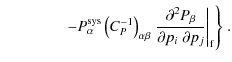
Dividing (B.6) by 2 yields the Fisher matrix, so that in the case of a biased
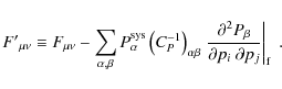
We want to determine the bias ![]() ,
where
,
where ![]() is the point in parameter space where the biased
is the point in parameter space where the biased ![]() attains its minimum. The biased parameter set
attains its minimum. The biased parameter set ![]() is computed from (B.4),
using the expansion up to second order, which results in
is computed from (B.4),
using the expansion up to second order, which results in

where the derivative of the
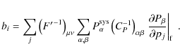
If one assumes that the systematic is small such that the second term in (B.7) becomes subdominant, (B.9) reproduces the known bias formula (29).
In summary, the differences in employing the exact likelihood/
![]() formalism (B.1)
or the Fisher matrix approach (28, 29) can be
reduced to cutting the Taylor expansion in (B.4)
after the second order in
formalism (B.1)
or the Fisher matrix approach (28, 29) can be
reduced to cutting the Taylor expansion in (B.4)
after the second order in ![]() ,
and dropping the second term in (B.7).
Both approximations are fair if the amplitude of the systematic and the
bias it produces are sufficiently small.
,
and dropping the second term in (B.7).
Both approximations are fair if the amplitude of the systematic and the
bias it produces are sufficiently small.
To quantify the validity of these approximations in the context of this
work we create a cosmic shear tomography survey with Nz=10
redshift bins without photometric redshift errors. The GI signal is
calculated via the linear intrinsic alignment model, with a free
overall scaling of ![]() to control the amplitude of the systematic. The original GI model
corresponds to
to control the amplitude of the systematic. The original GI model
corresponds to ![]() .
We use
.
We use ![]() as the only parameter to be constrained, setting a fiducial value of
0.4 for this exemplary analysis. Thereby, as the GI signal biases
as the only parameter to be constrained, setting a fiducial value of
0.4 for this exemplary analysis. Thereby, as the GI signal biases
![]() low, we allow for large biases in a range of still reasonable parameter
values. To achieve a suitable magnitude of statistical errors, the
survey size is set to
low, we allow for large biases in a range of still reasonable parameter
values. To achieve a suitable magnitude of statistical errors, the
survey size is set to ![]() and
and ![]() ,
respectively, the remaining parameters kept at the values given in
Sect. 3.
The exact errors are calculated via (B.1)
on a grid in parameter space with steps of 10-4
between
,
respectively, the remaining parameters kept at the values given in
Sect. 3.
The exact errors are calculated via (B.1)
on a grid in parameter space with steps of 10-4
between ![]() and
and ![]() .
While the minimum
.
While the minimum ![]() is simply read off the grid values, the
is simply read off the grid values, the ![]() -errors are computed by linear
interpolation on the grid, with
-errors are computed by linear
interpolation on the grid, with ![]() from the minimum for one degree of freedom.
from the minimum for one degree of freedom.
We define the ratios
where
![\begin{figure}
\par\includegraphics[scale=.6]{12420f18.ps}
\end{figure}](/articles/aa/full_html/2009/43/aa12420-09/img440.png)
|
Figure 16:
Comparison of statistical errors and biases obtained by Fisher matrix
and |
| Open with DEXTER | |
For ![]() ,
i.e. the default GI signal, we find a deviation of the bias obtained by
the Fisher matrix formalism of only
,
i.e. the default GI signal, we find a deviation of the bias obtained by
the Fisher matrix formalism of only ![]() ,
despite the strong systematic. The true bias is less than
,
despite the strong systematic. The true bias is less than ![]() larger
throughout, even for a very large systematic that dominates the signal
by far. In the analysis considered here, both the curvature of the GG
power spectrum and the systematic power spectrum are negative, so that
the second term in (B.7)
should in general be negative, too. Consequently, F'<F,
causing (B.9)
to produce larger biases than (29), which is
evident in Fig. B.1.
larger
throughout, even for a very large systematic that dominates the signal
by far. In the analysis considered here, both the curvature of the GG
power spectrum and the systematic power spectrum are negative, so that
the second term in (B.7)
should in general be negative, too. Consequently, F'<F,
causing (B.9)
to produce larger biases than (29), which is
evident in Fig. B.1.
If the amplitude of the systematic increases, the second term
in (B.7)
becomes more important, thereby leading to a scaling of the bias with
less than ![]() in (B.9).
Hence, the ratio of biases can curb down for large
in (B.9).
Hence, the ratio of biases can curb down for large ![]() because the bias, as computed from (29),
continues to scale with
because the bias, as computed from (29),
continues to scale with ![]() ,
an effect which is also seen in the figure. A similar behavior may be
expected from the inclusion of the third-order in (B.4)
as it leads to a term with bias squared in (B.8),
thereby placing the term scaling with
,
an effect which is also seen in the figure. A similar behavior may be
expected from the inclusion of the third-order in (B.4)
as it leads to a term with bias squared in (B.8),
thereby placing the term scaling with ![]() under a square root when solving for
under a square root when solving for ![]() .
.
In the presence of a bias a more accurate way to obtain statistical
errors than using the original Fisher matrix would be via F'.
As opposed to the Fisher matrix formalism, the statistical errors
become dependent on the systematic. Inspecting (B.7),
errors scale linearly with ![]() and should increase because of F'<F.
Again Fig. B.1
demonstrates that this holds true to good approximation, yielding
already a 8% effect at
and should increase because of F'<F.
Again Fig. B.1
demonstrates that this holds true to good approximation, yielding
already a 8% effect at ![]() .
Downscaling the systematic to
.
Downscaling the systematic to ![]() ,
the bias formalism should produce results that are very close to the
full likelihood calculation, even for the full set of cosmological
parameters.
,
the bias formalism should produce results that are very close to the
full likelihood calculation, even for the full set of cosmological
parameters.
References
- Abdalla, F., Amara, A., Capak, P., et al. 2007, MNRAS, 387, 969 [CrossRef] [NASA ADS]
- Albrecht, A., Bernstein, G., Cahn, R., et al. 2006 [arXiv:astro-ph/0609591]
- Amara, A., & Refregier, A. 2007, MNRAS, 381, 1018 [CrossRef] [NASA ADS]
- Amara, A., & Refregier, A. 2008, MNRAS, 391, 228 [CrossRef] [NASA ADS]
- Bacon, D., Refregier, A., & Ellis, R. 2000, MNRAS, 318, 625 [CrossRef] [NASA ADS]
- Benjamin, J., Heymans, C., Semboloni, E., et al. 2007, MNRAS, 381, 702 [CrossRef] [NASA ADS]
- Bernstein, G. 2009, ApJ, 695, 652 [CrossRef] [NASA ADS]
- Brainerd, T., Agustsson, I., Madsen, C., et al. 2009, ApJ, submitted [arXiv:0904.3095]
- Bridle, S., & Abdalla, F. 2007, ApJ, 655, L1 [CrossRef] [NASA ADS]
- Bridle, S., Balan, S., Bethge, M., et al. 2009, MNRAS, submitted [arXiv:0908.0945]
- Bridle, S., & King, L. 2007, NJPh, 9, 444 [CrossRef] [NASA ADS]
- Brown, M., Taylor, A., Hambly, N., et al. 2002, MNRAS, 333, 501 [CrossRef] [NASA ADS]
- Catelan, P., Kamionkowski, M., & Blandford, R. 2001, MNRAS, 320, 7 [CrossRef] [NASA ADS]
- Crittenden, R., Natarajan, P., Pen, U., et al. 2001, ApJ, 559, 552 [CrossRef] [NASA ADS]
- Croft, R., & Metzler, C. 2000, ApJ, 545, 561 [CrossRef] [NASA ADS]
- Eifler, T., Schneider, P., & Hartlap, J. 2009, A&A, 502, 721 [EDP Sciences] [CrossRef] [NASA ADS]
- Eisenstein, D., & Hu, W. 1998, ApJ, 496, 605 [CrossRef] [NASA ADS]
- Fu, L., Semboloni, E., Hoekstra, H., et al. 2008, A&A, 479, 9 [EDP Sciences] [CrossRef] [NASA ADS]
- Heavens, A. 2009, in Lecture Notes in Physics, ed. V. J. Martínez, E. Saar, E. Martínez-González, M.-J. Pons-Bordería (Berlin: Springer Verlag), 665, 585
- Heavens, A., Refregier, A., & Heymans, C. 2000, MNRAS, 319
- Hetterscheidt, M., Simon, P., Schirmer, M., et al. 2007, A&A, 468, 859 [EDP Sciences] [CrossRef] [NASA ADS]
- Heymans, C., & Heavens, A. 2003, MNRAS, 339, 711 [CrossRef] [NASA ADS]
- Heymans, C., Brown, M., Heavens, A., et al. 2004, MNRAS, 347, 895 [CrossRef] [NASA ADS]
- Heymans, C., van Waerbeke, L., Bacon, D., et al. 2006, MNRAS, 368, 1323 [CrossRef] [NASA ADS]
- Hirata, C., & Seljak, U. 2004, Phys. Rev. D, 70, 063526 [CrossRef] [NASA ADS] (HS04)
- Hirata, C., Mandelbaum, R., Ishak, M., et al. 2007, MNRAS, 381, 1197 [CrossRef] [NASA ADS]
- Hoekstra, H., & Jain, B. 2008, Ann. Rev. Nucl. Part. Sc., 58, 99 [CrossRef] [NASA ADS]
- Hoekstra, H., Mellier, Y., van Waerbeke, L., et al. 2006, ApJ, 647, 116 [CrossRef] [NASA ADS]
- Hu, W. 1999, ApJ, 522, 21 [CrossRef] [NASA ADS]
- Hu, W. 2002, Phys. Rev. D, 65, 023003 [CrossRef] [NASA ADS]
- Hu, W., & Jain, B. 2004, Phys. Rev. D, 70, 043009 [CrossRef] [NASA ADS]
- Huterer, D., & Takada, M. 2005, APh, 23, 369 [NASA ADS]
- Huterer, D., Takada, M., Bernstein, G., et al. 2006, MNRAS, 366, 101 [NASA ADS]
- Ilbert, O., Capak, P., Salvato, M., et al. 2009, ApJ, 690, 1236 [CrossRef] [NASA ADS]
- Jarvis, M., Jain, B., Bernstein, G., et al. 2006, ApJ, 644, 71 [CrossRef] [NASA ADS]
- Jing, Y. 2002, MNRAS, 335, 89 [CrossRef] [NASA ADS]
- Joachimi, B., & Schneider, P. 2008, A&A, 488, 829 [EDP Sciences] [CrossRef] [NASA ADS] (JS08)
- Joachimi, B., Schneider, P., & Eifler, T. 2008, A&A, 477, 43 [EDP Sciences] [CrossRef] [NASA ADS]
- Kaiser, N. 1992, ApJ, 388, 272 [CrossRef] [NASA ADS]
- Kaiser, N., Wilson, G., & Luppino, G. 2000 [arXiv:astro-ph/0003338]
- Kim, A., Linder, E., Miquel, R., et al. 2004, MNRAS, 347, 909 [CrossRef] [NASA ADS]
- King, L. 2005, A&A, 441, 47 [EDP Sciences] [CrossRef] [NASA ADS]
- King, L., & Schneider, P. 2002, A&A, 396, 411 [EDP Sciences] [CrossRef] [NASA ADS]
- King, L., & Schneider, P. 2003, A&A, 398, 23 [EDP Sciences] [CrossRef] [NASA ADS]
- Kitching, T., Amara, A., Abdalla, F., Joachimi, B., & Refregier, A. 2009, MNRAS, accepted
- Lee, J., & Pen, U.-L. 2000, ApJ, 532, L5 [CrossRef] [NASA ADS]
- Ma, Z., Hu, W., & Huterer, D. 2006, ApJ, 636, 21 [CrossRef] [NASA ADS]
- Mackey, J., White, M., & Kamionkowski, M. 2002, MNRAS, 332, 788 [CrossRef] [NASA ADS]
- Mandelbaum, R., Hirata, C., Ishak, M., Seljak, U., & Brinkmann, J. 2006, MNRAS, 367, 611 [CrossRef] [NASA ADS]
- Massey, R., Heymans, C., Berge, J., et al. 2007, MNRAS, 376, 13 [CrossRef] [NASA ADS]
- Munshi, D., Valageas, P., van Waerbeke, L., et al. 2008, PhR, 462, 67 [NASA ADS]
- Okumura, T., & Jing, Y. 2009, ApJ, 694, L83 [CrossRef] [NASA ADS]
- Okumura, T., Jing, Y., & Li, C. 2009, ApJ, 694, 214 [CrossRef] [NASA ADS]
- Peacock, J., & Dodds, S. 1996, MNRAS, 280, L19 [NASA ADS]
- Peacock, J., Schneider, P., Efstathiou, G., et al. 2006, in ESA-ESO Working Group on ''Fundamental Cosmology'', ed. G. J.A. Peacock et al., ESA
- Pen, U.-L., Lee, J., & Seljak, U. 2000, ApJ, 543, L107 [CrossRef] [NASA ADS]
- Schäfer, B. 2009, IJMPD, 18, 173 [CrossRef] [NASA ADS]
- Schäfer, B., Caldera-Cabral, G., & Maartens, R. 2008, MNRAS, submitted [arXiv:0803.2154]
- Schneider, M., & Bridle, S. 2009, PRD, submitted [arXiv:0903.3870]
- Schneider, P. 2003, A&A, 408, 829 [EDP Sciences] [CrossRef] [NASA ADS]
- Schneider, P. 2006, in Saas-Fee Advanced Course 33: Gravitational Lensing: Strong, Weak and Micro, ed. G. Meylan, P. Jetzer, P. North, P. Schneider, C. S. Kochanek, & J. Wambsganss, 269
- Semboloni, E., Mellier, Y., van Waerbeke, L., et al. 2006, A&A, 452, 51 [EDP Sciences] [CrossRef] [NASA ADS]
- Semboloni, E., Heymans, C., van Waerbeke, L., et al. 2008, MNRAS, 388, 991 [CrossRef] [NASA ADS]
- Simon, P., King, L., & Schneider, P. 2004, A&A, 417, 873 [EDP Sciences] [CrossRef] [NASA ADS]
- Smail, I., Ellis, R., & Fitchett, M. 1994, MNRAS, 270, 245 [NASA ADS]
- Spergel, D., Bean, R., Doré, O., et al. 2007, ApJS, 170, 377 [CrossRef] [NASA ADS]
- Sugiyama, N. 1995, ApJS, 100, 281 [CrossRef] [NASA ADS]
- Taburet, N., Aghanim, N., Douspis, M., et al. 2009, MNRAS, 392, 1153 [CrossRef] [NASA ADS]
- Takada, M., & White, M. 2004, ApJ, 601, 1 [CrossRef] [NASA ADS]
- Taylor, A., Kitching, T., Bacon, D., et al. 2007, MNRAS, 374, 1377 [CrossRef] [NASA ADS]
- Tegmark, M., Taylor, A., & Heavens, A. 1997, ApJ, 480, 22 [CrossRef] [NASA ADS]
- Thomas, S., Abdalla, F., & Weller, J. 2009, MNRAS, 395, 197 [CrossRef] [NASA ADS]
- van den Bosch, F., Abel, T., Croft, R., Hernquist, L., & White, S. 2002, ApJ, 576, 21 [CrossRef] [NASA ADS]
- van Waerbeke, L., Mellier, Y., Erben, T., et al. 2000, A&A, 358, 30 [NASA ADS]
- Wittman, D., Tyson, J., Kirkman, D., Antonio, I. D., & Bernstein, G. 2000, Nature, 405, 143 [CrossRef] [NASA ADS]
- Zhang, P. 2008, ApJ, submitted [arXiv:0811.0613]
Footnotes
- ... cases
![[*]](/icons/foot_motif.png)
- Note however that the total power spectrum of auto-correlations of ellipticities, i.e. GG+GI+II, always has to be positive by definition.
- ... distribution
- For perfect correspondence the lower limit of the integral
over
 should be
  instead of
  .
However, the nulling weight given as
.
However, the nulling weight given as
 has to vanish for
  ,
and at the same time the outer integral ensures
,
and at the same time the outer integral ensures
 .
.
- ...)
- This referring is merely for illustrative purposes and not part of the procedure outlined above.
- ... reads
- Note that there is a typo in Eq. (14) of Tegmark et al. (1997): A factor C-1 should be eliminated from the last term.
All Tables
Table 1: Upper limits on the allowed angular frequency range if the II contamination in the nulled data shall be suppressed by at least a factor of s with respect to the nulled GG term.
Table 2: Overview on nulling variants considered.
Table
3: Errors on cosmological parameters for three exemplary data
sets with different photometric redshift errors. Top:
ratios rF
and rb
for the three data sets considered. Bottom:
marginalized statistical errors ![]() ,
biases b, total errors
,
biases b, total errors ![]() ,
and
,
and ![]() for every cosmological parameter, shown for both original and nulled
data sets.
for every cosmological parameter, shown for both original and nulled
data sets.
Current usage metrics show cumulative count of Article Views (full-text article views including HTML views, PDF and ePub downloads, according to the available data) and Abstracts Views on Vision4Press platform.
Data correspond to usage on the plateform after 2015. The current usage metrics is available 48-96 hours after online publication and is updated daily on week days.
Initial download of the metrics may take a while.