| Issue |
A&A
Volume 507, Number 1, November III 2009
|
|
|---|---|---|
| Page(s) | 53 - 59 | |
| Section | Cosmology (including clusters of galaxies) | |
| DOI | https://doi.org/10.1051/0004-6361/200911998 | |
| Published online | 08 September 2009 | |
A&A 507, 53-59 (2009)
Probing the cosmographic parameters to
distinguish between dark energy and modified gravity models
(Research Note)
F. Y. Wang1,2 - Z. G. Dai1 - Shi Qi3,4
1 - Department of Astronomy, Nanjing University, Nanjing 210093, PR
China
2 - Department of Astronomy, University of Texas at Austin, Austin, TX
78712, USA
3 - Purple Mountain Observatory, Chinese Academy of Sciences, Nanjing
210008, PR China
4 - Joint Center for Particle, Nuclear Physics and Cosmology, Nanjing
University - Purple Mountain Observatory, Nanjing 210093, PR China
Received 6 March 2009 / Accepted 4 August 2009
Abstract
Aims. In this paper we investigate the deceleration,
jerk and
snap parameters to distinguish between the dark energy and modified
gravity models using high redshift gamma-ray bursts (GRBs) and
supernovae (SNe).
Methods. We first derive the expressions of
deceleration, jerk
and snap parameters in dark energy and modified gravity models. In
order to constrain the cosmographic parameters, we calibrate the GRB
luminosity relations without assuming any cosmological models using SNe
Ia. Then we constrain the model parameters (including dark energy and
modified gravity models) using type Ia supernovae and gamma-ray bursts.
Finally we calculate the cosmographic parameters. GRBs can extend the
redshift-distance relation up to high redshifts, because they can be
detected to high redshifts.
Results. We find that the statefinder pair (r,s)
could not be used to distinguish between some dark energy and modified
gravity models, but these models could be differentiated by the snap
parameter. Using the model-independent constraints on cosmographic
parameters, we conclude that the ![]() CDM model is consistent with
current data.
CDM model is consistent with
current data.
Key words: gamma rays: bursts - cosmology: cosmological parameters - cosmology: distance scale
1 Introduction
Recent observations of the Hubble relation of distant type Ia
supernovae (SNe Ia) have provided strong evidence for acceleration of
the present universe (Riess et al. 1998;
Perlmutter et al. 1999).
The observations of the spectrum of cosmic microwave background (CMB)
anisotropies (Spergel et al. 2003, 2007),
large-scale structure
(LSS) (Tegmark et al. 2004; Eisenstein
et al. 2005)
and the distance-redshift relation to X-ray galaxy clusters (Allen
et al. 2004, 2007)
also confirm that the universe is accelerating. Possible explanations
for this acceleration have been proposed. A negative pressure term
called dark energy is taken into account, such as in the cosmological
constant model with equation of state
![]() (Weinberg 1989),
an evolving scalar field (Peeble & Ratra 1988;
Caldwell et al. 1998),
phantom energy for which the sum of the pressure and energy density is
negative, and the Chaplygin gas (Kamenshchik et al. 2001).
All the above models for acceleration are obtained by introducing a new
energy component called dark energy. Alternative models, in which
gravity is modified, can also drive the universe acceleration, e.g.,
the Dvali-Gabadadze-Porrati (DGP) model (Dvali et al. 2000;
Deffayet et al. 2002),
Cardassian expansion model (Freese & Lewis 2002; Wang
et al. 2003), and
the f(R) gravity model (Vollick 2003;
Carroll et al. 2004).
(Weinberg 1989),
an evolving scalar field (Peeble & Ratra 1988;
Caldwell et al. 1998),
phantom energy for which the sum of the pressure and energy density is
negative, and the Chaplygin gas (Kamenshchik et al. 2001).
All the above models for acceleration are obtained by introducing a new
energy component called dark energy. Alternative models, in which
gravity is modified, can also drive the universe acceleration, e.g.,
the Dvali-Gabadadze-Porrati (DGP) model (Dvali et al. 2000;
Deffayet et al. 2002),
Cardassian expansion model (Freese & Lewis 2002; Wang
et al. 2003), and
the f(R) gravity model (Vollick 2003;
Carroll et al. 2004).
These two families of models, dark energy and modified gravity, are fundamentally different. An important question is whether it is possible to distinguish between the modified gravity and dark energy models that have nearly the same cosmic expansion history. Much work has been done on this topic. A usually-discussed quantity is the growth rate of cosmological density perturbations, which should be different in the models depending on different gravity theory even if they have an identical cosmic expansion history. Recently, there have been extensive discussions on discriminating dark energy and modified gravity models using the matter density perturbation growth factor (Linder 2005). But Kunz & Sapone (2007) demonstrated that the growth factor is not sufficient to distinguish between modified gravity and dark energy (Kunz & Sapone 2007). They found that a generalized dark energy model can match the growth rate of the Dvali-Gabadadze-Porrati model and reproduce the 3+1 dimensional metric perturbations.
On the other hand, the statefinder pair (r,s)
has also been proposed to distinguish between the models, where ![]() and
and ![]() .
Sahni et al. (2003)
demonstrated that the statefinder diagnostic could effectively
discriminate different forms of dark energy (Sahni et al. 2003). Alam
et al. (2003)
investigated the cosmological constant, quintessence, Chaplygin gas,
and braneworld models using the statefinder diagnostic, and found that
the statefinder pair could differentiate between these models (Alam
et al. 2003).
Different cosmological models exhibit qualitatively different
trajectories of evolution in the r-s
plane. The statefinder diagnostic has been extensively used in many
models (Gorini et al. 2003). But
the statefinder pair is difficult to measure with cosmological
observations (Visser 2004;
Cattoën & Visser 2007).
.
Sahni et al. (2003)
demonstrated that the statefinder diagnostic could effectively
discriminate different forms of dark energy (Sahni et al. 2003). Alam
et al. (2003)
investigated the cosmological constant, quintessence, Chaplygin gas,
and braneworld models using the statefinder diagnostic, and found that
the statefinder pair could differentiate between these models (Alam
et al. 2003).
Different cosmological models exhibit qualitatively different
trajectories of evolution in the r-s
plane. The statefinder diagnostic has been extensively used in many
models (Gorini et al. 2003). But
the statefinder pair is difficult to measure with cosmological
observations (Visser 2004;
Cattoën & Visser 2007).
The present values of cosmographic parameters can be determined from
observations (Riess et al. 2004;
Visser 2004).
Caldwell & Kamionkowski (2004)
showed that the jerk parameter could probe the spatial curvature of the
universe (Caldwell & Kamionkowski 2004).
The deceleration, jerk and snap parameters are related to the second,
third and fourth derivative of the scale factor respectively. Visser (2004)
expanded the Hubble law to fourth order in redshift including the snap
parameter and put constraints on the deceleration and jerk parameters
using SNe Ia (Visser 2004).
Rapetti et al. (2007)
constrained the deceleration and jerk parameters from SNe Ia and X-ray
cluster gas mass fraction measurements. For a redshift range of SNe Ia,
the terms beyond the cubic power of the Hubble law can be neglected. In
order to put a narrow constraint on the snap parameter, we need
high-redshift objects. GRBs may be a useful tool. GRBs can be
detectable out to very high redshifts
(Ciardi & Loeb 2000). The
farthest burst detected so far is GRB 090423, which is at z=8.2
(Olivares et al. 2009). A
lot of work in this so-called GRB cosmology has
been published (Dai et al. 2004;
Ghirlanda et al. 2004;
Di Girolamo et al. 2005;
Firmani et al. 2005;
Friedman & Bloom 2005;
Lamb et al. 2005; Liang
& Zhang 2005, 2006; Xu
et al. 2005; Wang
& Dai 2006;
Schaefer 2007;
Wright 2007; Wang
et al. 2007; Gong
& Chen 2007; Li et al. 2008; Liang
et al. 2008; Qi
et al. 2008a,b;
Basilakos &
Perivolaropoulos 2008;
Kodama et al. 2008; Wang
et al. 2009). Very
recently, Schaefer (2007)
used 69 GRBs and five relations to
build the Hubble diagram out to z=6.60 and
discussed the properties of dark energy in several dark energy models
(Schaefer 2007).
He found that the GRB Hubble diagram is consistent with the concordance
cosmology. Liang et al. (2008)
calibrated the luminosity relations of GRBs by interpolating from the
Hubble diagram of SNe Ia at z<1.4 with the
assumption that objects at the same redshift should have the same
luminosity distance (Liang et al. 2008). This
method is model-independent. More recently, Capozziello & Izzo (2008)
used the Liang et al. (2008)
results to constrain the cosmographic parameters and found that the
results calibrated by SNe Ia data agree with the ![]() CDM model. Cardone
et al. (2009)
used 83 GRBs and six correlations to build the Hubble diagram.
CDM model. Cardone
et al. (2009)
used 83 GRBs and six correlations to build the Hubble diagram.
Riess et al. (2004)
found that the jerk j0
is positive at the 92% confidence level based on their ``gold'' dataset
and is positive at the 95% confidence level based on their
``gold+silver'' dataset. Neither explicit upper bounds are given for
the jerk nor are any constraints placed on the snap s0.
Rapetti et al. (2007)
measured ![]() and
and ![]() in a flat model with constant jerk (Rapetti et al. 2007).
Capozziello & Izzo (2008)
used 27 GRBs to derive the values of the cosmographic
parameters. They found
in a flat model with constant jerk (Rapetti et al. 2007).
Capozziello & Izzo (2008)
used 27 GRBs to derive the values of the cosmographic
parameters. They found ![]() ,
,
![]() and
and ![]() .
In this paper, we use more GRB data to constrain the cosmography
parameters in several dark energy and modified gravity models.
.
In this paper, we use more GRB data to constrain the cosmography
parameters in several dark energy and modified gravity models.
We calibrate the luminosity relations of GRBs using SNe Ia and calculate the deceleration, jerk and snap parameters of several dark energy and modified gravity models using SNe Ia and GRBs. We also use a model-independent method to constrain the cosmographic parameters. We find that in some models the jerk parameters are almost equal to each other. So this parameter is not used to distinguish between the models. However, the snap parameters in all the models are different, so we can distinguish between the models using the snap parameter.
The structure of this paper is as follows. In Sect. 2 we introduce the Hubble, deceleration, jerk and snap parameters. In Sect. 3 we derive expressions of cosmographic parameters of the Hubble law in several dark energy models. In Sect. 4 we present expressions of cosmographic parameters of the Hubble law in modified gravity models. The constraints on model parameters and cosmographic parameters of the Hubble law are given in Sect. 5. Finally, Sect. 6 contains conclusions and discussions.
2 Hubble, deceleration, jerk and snap parameters
The expansion rate of the Universe can be written in terms of the
Hubble parameter, ![]() ,
where a is the scale factor and
,
where a is the scale factor and ![]() is its first derivative with respect to time. As we known that q
is the deceleration parameter, related to the second derivative of the
scale factor, j is the so-called ``jerk'' or
statefinder parameter, related to the third derivative of the scale
factor, and s
is the so-called ``snap'' parameter, which is related to the fourth
derivative of the scale factor. These quantities are
defined as
is its first derivative with respect to time. As we known that q
is the deceleration parameter, related to the second derivative of the
scale factor, j is the so-called ``jerk'' or
statefinder parameter, related to the third derivative of the scale
factor, and s
is the so-called ``snap'' parameter, which is related to the fourth
derivative of the scale factor. These quantities are
defined as

|
(1) |

|
(2) |

|
(3) |
The deceleration, jerk and snap parameters are dimensionless, and a Taylor expansion of the scale factor around t0 provides
| a(t) | = | 
|
|
![$\displaystyle +\frac{1}{4!}s_0H_{0}^{4}(t-t_0)^4+O\left[(t-t_0)^5\right]\bigg\},$](/articles/aa/full_html/2009/43/aa11998-09/img19.png)
|
(4) |
and so the luminosity distance
|
|
= | 
|
|

|
(5) |
(Visser 2004). For the redshift range of SNe Ia the terms beyond the cubic power in Eq. (5) can be neglected. If models have the same deceleration and jerk parameters, we can see degeneracy of these models from Eq. (5). Therefore we must measure the snap parameters to distinguish between the models. This needs high-redshift objects. The relations among the q(z),j(z) and s(z) are
|
(6) |
|
(7) |
The Friedmann equation is
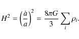
|
(8) |
From Einstein's equations, we can obtain the dynamical equation of the universe
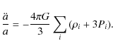
The conservation equation is
| (10) |
In order to derive the jerk and snap parameter, we differentiate Eq. (9)
|
|
= | ||
| = | |||
| (11) |
|
|
= | ||
| = | |||
| (12) |
3 Dark energy models
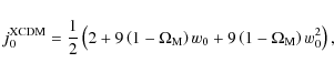
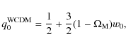
3.1 w(z) parameterization model
We first consider the dark energy with a constant equation of state
| w(z)=w0. | (13) |
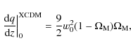
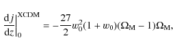
For this model, we obtain
![\begin{displaymath}%
q_0^{\rm XCDM}={3 \over
2}\left[1+w_0(1- \Omega_{\rm M})\right]-1,
\end{displaymath}](/articles/aa/full_html/2009/43/aa11998-09/img37.png)
|
(14) |
|
(15) |
|
(16) |
|
(17) |
|
|
= | ||
| (18) |
These expressions are consistent with Bertolami & Silva (2006).
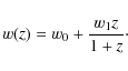
A more interesting approach to explore dark energy is to use a
time-dependent dark energy model. The simplest parameterization
including two parameters is (Maor et al. 2001; Weller
& Albrecht 2001)
| w(z)=w0+w1z. | (19) |
In this dark energy model the luminosity distance is (Linder 2003)
|
|
= | 
|
|
| (20) |
The cosmographic parameters are:
|
(21) |
|
|
= | ||
| (22) |
|
|
= | ||
| (23) |
We consider the Chevallier-Polarski-Linder parameterization (Chevallier & Polarski 2001; Linder 2003)
|
(24) |
The luminosity distance is (Chevallier & Polarski 2001; Linder 2003)
|
|
= |
|
|
| (25) |
The cosmographic parameters are:
|
(26) |
|
|
= | ||
| (27) |
|
|
= | ||
| (28) |
Capozziello et al. (2008) and Capozziello & Izzo (2008) also derived cosmographic parameters in this model. Our results are consistent with theirs.
3.2 Generalized Chaplygin gas model
We consider the generalized Chaplygin gas (GCG) model, which is
characterized by the equation of state
|
(29) |
We can integrate the conservation equation for generalized Chaplygin gas, leading to
![\begin{displaymath}%
\rho_{\rm GCG}=\rho_{\rm
GCG0}\left[A_s+(1-A_s)a^{-3(1+\alpha)}\right]^{1/(1+\alpha)}
\end{displaymath}](/articles/aa/full_html/2009/43/aa11998-09/img63.png)
where
|
(31) |
where
|
|
= | ||
| (32) |
|
|
= | 
|
|
| (33) |
For the GCG model we obtain (Bertolami & Silva 2006; Wang et al. 2009)
|
(34) |
|
(35) |
|
(36) |
|
(37) |
| (38) |
4 Modified gravity models
4.1 Cardassian expansion model
The original Cardassian model was first introduced in Freese &
Lewis (2002)
as a possible alternative to explain the acceleration of the universe.
They modified the Friedmann equation as
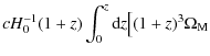
This model has no energy component besides ordinary matter. If we consider a spatially flat FRW universe, the Friedmann equation is modified as Eq. (39). The universe undergoes acceleration requiring n < 2/3. If n=0, it is the same as the cosmological constant universe. We can obtain H(z) by using Eq. (39) and
![\begin{displaymath}%
H(z)^2=H_0^2\left[\Omega_{\rm m}(1+z)^3+(1-\Omega_{\rm m})(1+z)^{3n}\right],
\end{displaymath}](/articles/aa/full_html/2009/43/aa11998-09/img80.png)
where
![\begin{displaymath}%
d_{\rm L}=cH_{0}^{-1}(1\!+\!z)\int_{0}^{z}{\rm d}z\left[(1\...
...ga_{\rm m}+(1\!-\!\Omega_{\rm m})(1\!+\!z)^{3n}\right]^{-1/2}.
\end{displaymath}](/articles/aa/full_html/2009/43/aa11998-09/img82.png)
|
(41) |
For the Cardassian expansion model, we obtain
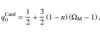
|
(42) |
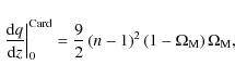
|
(43) |
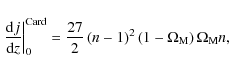
|
(44) |
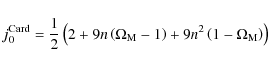
|
(45) |
|
|
= | ||
| (46) |
4.2 Dvali-Gabadadze-Porrati model
In the DGP model the modified Friedmann equation due to the
presence
of an infinite-volume extra dimension is (Deffayet et al. 2002)
![\begin{displaymath}%
H^2 = H_0^2 \left[\Omega_k(1+z)^2+\left(\sqrt{\Omega_{r_{\r...
...t{\Omega_{r_{\rm c}}+\Omega_{\rm m} (1+z)^3}\right)^2 \right],
\end{displaymath}](/articles/aa/full_html/2009/43/aa11998-09/img90.png)
where the bulk-induced term,

For a flat universe,
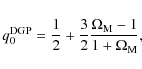
|
(49) |
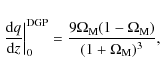
|
(50) |
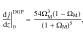
|
(51) |
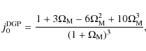
|
(52) |
|
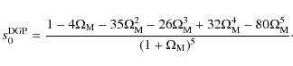
(53) |
4.3 f(R) gravity
f(R) gravity models, in which the
gravitational Lagrangian is a function of the curvature scalar R,
also can explain the current cosmic acceleration (Vollick 2003;
Carroll et al. 2004;
Capozziello et al. 2009).
Poplawski (2006)
derived a quite complicated expression for the jerk parameter in ![]() (Poplawski
2006):
(Poplawski
2006):
The snap parameter in this model is (Poplawski 2007)
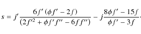
Poplawski (2007) calculated
5 Constraints from SNe Ia and GRBs
Davis et al. (2007)
fitted the SNe Ia dataset that includes 60 ESSENCE SNe Ia (WoodVasey
et al. 2007),
57 SNe Ia from Super-Nova Legacy Survey (SNLS) (Astier
et al. 2006), 45
nearby SNe Ia and 30 SNe Ia detected by HST (Riess
et al. 2007) with
the MCLS2K2 method. With the luminosity distance ![]() in units of megaparsecs, the
predicted distance modulus is
in units of megaparsecs, the
predicted distance modulus is
| (56) |
The likelihood functions can be determined from the
![\begin{displaymath}%
\chi^{2}_{\rm SNe}=\sum_{i=1}^{N} \frac{\left[\mu_{i}(z_{i})-\mu_{0,i}\right]^{2}}{\sigma_{\mu_{0,i}}^{2}+\sigma_{\nu}^{2}},
\end{displaymath}](/articles/aa/full_html/2009/43/aa11998-09/img121.png)
|
(57) |
where
We use the calibration results obtained by using the
interpolation methods directly from SNe Ia data (Liang et al. 2008). The
calibrated luminosity relations are completely cosmology
independent. We assume that these relations do not evolve with redshift
and are valid in z>1.40.
The luminosity or energy of GRB can be calculated. Thus, the luminosity
distances and distance
modulus can be obtained. After obtaining the distance modulus of each
burst using one of these relations, we use the same method as Schaefer (2007) to
calculate the real distance modulus,
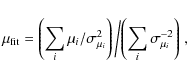
|
(58) |
where the summation runs from 1-5 over the relations with available data,
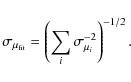
|
(59) |
The
![\begin{displaymath}%
\chi^{2}_{\rm GRB}=\sum_{i=1}^{N} \frac{\left[\mu_{i}(z_{i})-\mu_{{ fit},i}\right]^{2}}{\sigma_{\mu_{{\rm fit},i}}^{2}},
\end{displaymath}](/articles/aa/full_html/2009/43/aa11998-09/img130.png)
|
(60) |
where
We combine SNe Ia and GRBs by multiplying the likelihood
functions. The total ![]() value is
value is ![]() .
The best fitted value is obtained by
minimizing
.
The best fitted value is obtained by
minimizing ![]() .
.
5.1 Constraints on cosmographic parameters
In our analysis, we consider a flat cosmology. We use ![]() from the Hubble Space Telescope key projects
(Freedman et al. 2001).
from the Hubble Space Telescope key projects
(Freedman et al. 2001).
Let us first consider observational constraints on dark energy models.
In Fig. 1,
we show the distribution probabilities as a function of ![]() in the flat
in the flat ![]() CDM
model from SNe Ia and GRBs. From this figure, we have
CDM
model from SNe Ia and GRBs. From this figure, we have ![]() .
The cosmographic parameters in
.
The cosmographic parameters in ![]() CDM model are
CDM model are ![]() ,
j0=1.0 and
,
j0=1.0 and ![]() .
We can obtain
.
We can obtain ![]() ,
j0=1.0 and
,
j0=1.0 and ![]() .
.
![\begin{figure}
\par\includegraphics[width=7.5cm,clip]{11998fg1.eps}
\end{figure}](/articles/aa/full_html/2009/43/aa11998-09/img141.png)
|
Figure 1: Luminosity distance-redshift diagram. The circles are the GRBs. The solid line is the result of our fitting. |
| Open with DEXTER | |
![\begin{figure}
\par\includegraphics[width=7.5cm,clip]{11998fg2.eps}
\end{figure}](/articles/aa/full_html/2009/43/aa11998-09/img142.png)
|
Figure 2:
Constraints on |
| Open with DEXTER | |
In Fig. 2
we present constraints on ![]() and w from
and w from ![]() to
to ![]() using 192 SNe Ia and 69 GRBs in the w=w0
model. We measure
using 192 SNe Ia and 69 GRBs in the w=w0
model. We measure ![]() and
and ![]() .
The cosmographic parameters in the w=w0
model are
.
The cosmographic parameters in the w=w0
model are ![]() ,
,
![]() and
and
![]() .
.
In Fig. 3
we present constraints on w0
and w1 from ![]() to
to ![]() using 192 SNe Ia and 69 GRBs in the w=w0+w1
z model. The values of the parameters are
using 192 SNe Ia and 69 GRBs in the w=w0+w1
z model. The values of the parameters are ![]() and
and ![]() .
The cosmographic parameters are
.
The cosmographic parameters are ![]() ,
,
![]() and
and ![]() .
.
![\begin{figure}
\par\includegraphics[width=7.5cm,clip]{11998fg3.eps}
\end{figure}](/articles/aa/full_html/2009/43/aa11998-09/img153.png)
|
Figure 3: The same as Fig. 2 but in the w=w0+w1 z model. |
| Open with DEXTER | |
In Fig. 4
we present constraints on w0
and w1 from ![]() to
to ![]() using 192 SNe Ia and 69 GRBs in the w=w0+w1
z/(1+z) model. We measure
using 192 SNe Ia and 69 GRBs in the w=w0+w1
z/(1+z) model. We measure ![]() and
and ![]() .
The cosmographic parameters are
.
The cosmographic parameters are ![]() ,
,
![]() and
and ![]() .
.
![\begin{figure}
\par\includegraphics[width=7.5cm,clip]{11998fg4.eps}
\end{figure}](/articles/aa/full_html/2009/43/aa11998-09/img159.png)
|
Figure 4: The same as Fig. 2 but in the w=w0+w1 z/(1+z) model. |
| Open with DEXTER | |
Figure 5
shows constraints on As
and ![]() from
from ![]() to
to ![]() using SNe Ia and GRBs in the GCG model. The parameters are
using SNe Ia and GRBs in the GCG model. The parameters are ![]() and
and ![]() .
The cosmographic parameters are
.
The cosmographic parameters are ![]() ,
,
![]() and
and ![]() .
.
![\begin{figure}
\par\includegraphics[width=7.5cm,clip]{11998fg5.eps}
\end{figure}](/articles/aa/full_html/2009/43/aa11998-09/img166.png)
|
Figure 5: The same as Fig. 2 but in the GCG model. |
| Open with DEXTER | |
In Fig. 6
we present constraints on ![]() and n from
and n from ![]() to
to ![]() using 192 SNe Ia and 69 GRBs in the Cardassian
expansion model. We measure
using 192 SNe Ia and 69 GRBs in the Cardassian
expansion model. We measure ![]() and
and ![]() .
The cosmographic parameters are
.
The cosmographic parameters are ![]() ,
,
![]() and
and
![]() .
.
![\begin{figure}
\par\includegraphics[width=7.5cm,clip]{11998fg6.eps}
\end{figure}](/articles/aa/full_html/2009/43/aa11998-09/img172.png)
|
Figure 6: The same as Fig. 2 but in the Cardassian expansion model. |
| Open with DEXTER | |
Figure 7
shows constraints on ![]() using SNe Ia and GRBs in the DGP model. The value of
using SNe Ia and GRBs in the DGP model. The value of ![]() is
is ![]() .
The cosmographic parameters are
.
The cosmographic parameters are ![]() ,
,
![]() and
and ![]() .
.
![\begin{figure}
\par\includegraphics[width=7.5cm,clip]{11998fg7.eps}
\end{figure}](/articles/aa/full_html/2009/43/aa11998-09/img177.png)
|
Figure 7: The same as Fig. 1 but in the DGP model. |
| Open with DEXTER | |
We directly use Eq. (5) to constrain the cosmographic
parameters. This analysis uses the FRW metric only, so we have not
specified any gravitational theory yet. The luminosity distance only
depends on
redshift z and cosmographic parameters. So this
method is
fully model independent. We use the 192 SNe Ia and
69 GRBs
and find the best fit parameters are
![]() ,
,
![]() and
and
![]() .
The results are consistent with the flat
.
The results are consistent with the flat ![]() CDM model.
CDM model.
In Table 1
we summarize the constraints on cosmographic parameters. The
deceleration and jerk parameters in the w=w0,
GCG, Cardassian expansion and f(R)
models are almost the same in the ![]() confidence level. These values are consistent with the deceleration and
jerk parameters of the
confidence level. These values are consistent with the deceleration and
jerk parameters of the ![]() CDM
model in the
CDM
model in the ![]() confidence
level. So these models cannot be discriminated between by using the
present value of the statefinder pair. However the snap parameter in
all the models is different and thus can be used to discriminate
between the cosmological models. In the future, more data will give a
precise snap parameter in different models.
confidence
level. So these models cannot be discriminated between by using the
present value of the statefinder pair. However the snap parameter in
all the models is different and thus can be used to discriminate
between the cosmological models. In the future, more data will give a
precise snap parameter in different models.
Table 1: The cosmographic parameter values.
6 Discussions and conclusions
The cosmic acceleration could be due to unidentified dark
energy, or
a modification of general relativity (modified gravity). In this paper
we investigate the deceleration, jerk and snap parameters in modified
gravity and dark energy models. We calibrated the GRB luminosity
relations using SNe Ia without assuming any cosmological models.
Because gamma-ray bursts can be detected at high redshifts, we
calculated the deceleration, jerk and snap parameters using type Ia
supernovae and gamma-ray bursts. GRBs can extend the redshift-distance
relation up to high redshifts. We find that the deceleration and jerk
parameters in the w=w0,
GCG, Cardassian expansion and f(R)
models are almost the same at a ![]() confidence level. So these models cannot be discriminated between using
the present value of the statefinder pair. We found that the dark
energy models and modified gravity models could be distinguished
between by the snap parameter. Using the model-independent constraints
on cosmographic parameters, we found that the
confidence level. So these models cannot be discriminated between using
the present value of the statefinder pair. We found that the dark
energy models and modified gravity models could be distinguished
between by the snap parameter. Using the model-independent constraints
on cosmographic parameters, we found that the ![]() CDM model is consistent with
the current data.
CDM model is consistent with
the current data.
This work is supported by the National Natural Science Foundation of China (grants 10233010, 10221001 and 10873009) and the National Basic Research Program of China (973 program) No. 2007CB815404. F. Y. Wang was also supported by the Jiangsu Project Innovation for Ph.D. Candidates (CX07B-039z).
References
- Alam, U., Sahni, V., Deep Saini, T., & Starobinsky, A. A. 2003, MNRAS, 344, 1057 [CrossRef] [NASA ADS]
- Allen, S. W., Schmidt, R. W., Ebeling, H., Fabian, A. C., & van Speybroeck, L. 2004, MNRAS, 353, 457 [CrossRef] [NASA ADS]
- Allen, S. W., Rapetti, D. A., Schmidt, R. W., et al. 2008, MNRAS, 383, 879 [CrossRef] [NASA ADS]
- Astier, P., Guy, J., Regnault, N., et al. 2006, A&A, 447, 31 [EDP Sciences] [CrossRef] [NASA ADS]
- Bertolami, O., & Silva, P. T. 2006, MNRAS, 356, 1149 [NASA ADS]
- Basilakos, S., & Perivolaropoulos, L. 2008, MNRAS, 391, 411 [CrossRef] [NASA ADS]
- Bennett, C. L., Hill, R. S., Hinshaw, G., et al. 2003, ApJS, 148, 97 [CrossRef] [NASA ADS]
- Bento, M. C., Bertolami, O., & Sen, A. A. 2002, Phys. Rev. D, 66, 043507 [CrossRef] [NASA ADS]
- Caldwell, R. R., & Kamionkowski, M. 2004, JCAP, 0409, 009 [NASA ADS]
- Caldwell, R. R., Dave, R., & Steinhardt, P. J. 1998, Phys. Rev. Lett., 80, 1582 [CrossRef] [NASA ADS]
- Capozziello, S., & Izzo, L. 2008, A&A, 490, 31 [EDP Sciences] [CrossRef] [NASA ADS]
- Capozziello, S., Cardone, V. F., & Salzano, V. 2008, Phys. Rev. D, 78, 063504 [CrossRef] [NASA ADS]
- Capozziello, S., Elizalde, E., Nojiri, S., & Odintsov, S. D. 2009, Phys. Lett. B, 671, 193 [CrossRef] [NASA ADS]
- Cardone, V. F., Capozziello, S., & Dainotti, M. G. 2009, [arXiv:0901.3194]
- Carroll, S. M., et al. 2004, Phys. Rev. D, 70, 043528 [CrossRef] [NASA ADS]
- Cattoën, C, & Visser, M. 2007, [gr-qc/0703122v3]
- Chevallier, M., & Polarski, D. 2001, Int. J. Mod. Phys. D, 10, 213 [CrossRef] [NASA ADS]
- Dai, Z. G., Liang, E. W., & Xu, D. 2004, ApJ, 612, L101 [CrossRef] [NASA ADS]
- Davis, T. M., Mörtsell, E., Sollerman, J., et al. 2007, ApJ, 666, 716 [CrossRef] [NASA ADS]
- Deffayet, C., Dvali, G. R., & Gabadadze, G. 2002, Phys. Rev. D, 65, 044023 [CrossRef] [NASA ADS]
- Ciardi, B., & Loeb, A. 2000, ApJ, 540, 687 [CrossRef] [NASA ADS]
- Dvali, G. R., Gabadadze, G., & Porrati, M. 2000, Phys. Lett. B, 485, 208 [CrossRef] [NASA ADS]
- Di Girolamo, T., et al. 2005, JCAP, 4, 008 [NASA ADS]
- Eisenstein, D. J., Zehavi, I., Hogg, D. W., et al. 2005, ApJ, 633, 560 [CrossRef] [NASA ADS]
- Firmani, C., Ghisellini, G., Ghirlanda, G., & Avila-Reese, V. 2005, MNRAS, 360, L1 [CrossRef] [NASA ADS]
- Fenimore, E. E., & Ramirez-Ruiz, E. 2000, [arXiv:astro-ph/0004176]
- Freedman, W. L., Madore, B. F., Gibson, B. K., et al. 2001, ApJ, 553, 47 [CrossRef] [NASA ADS]
- Freese, K., & Lewis, M. 2002, Phys. Lett. B, 540, 1 [CrossRef] [NASA ADS]
- Friedmann, A. S., & Bloom, J. S. 2005, ApJ, 627, 1 [CrossRef] [NASA ADS]
- Ghirlanda, G., Ghisellini, G., Lazzati, D., & Firmani, C. 2004, ApJ, 613, L13 [CrossRef] [NASA ADS]
- Gorini, V., Kamenshchik, A., & Moschella, U. 2003, Phys. Rev. D, 67, 063509 [CrossRef] [NASA ADS]
- Huterer, D., & Linder, E. V. 2007, Phys. Rev. D, 75, 023519 [CrossRef] [NASA ADS]
- Ishak, M., Upadhye, A., & Spergel, D. N. 2006, Phys. Rev. D, 74, 043513 [CrossRef] [NASA ADS]
- Kamenshchik, A., Moschella, U., & Pasquier, V. 2001, Phys. Lett. B, 511, 265 [CrossRef] [NASA ADS]
- Kodama, Y., Yonetoku, D., Murakami, T., et al. 2008, MNRAS, 391, L1 [CrossRef] [NASA ADS]
- Kunz, M., & Sapone, D. 2007, Phys. Rev. Lett., 98, 121301 [CrossRef] [NASA ADS]
- Lamb, D. Q., Ricker, G. R., Lazzati, D., et al. 2005, [arXiv:astro-ph/0507362]
- Li, H., Su, M., Fan, Z., Dai, Z., & Zhang, X. 2008, Phys. Lett. B, 658, 95 [CrossRef] [NASA ADS]
- Liang, E. W., & Zhang, B. 2005, ApJ, 633, 611 [CrossRef] [NASA ADS]
- Liang, E. W., & Zhang, B. 2006, MNRAS, 369, L37 [NASA ADS]
- Liang, N., Ke Xiao, W., Liu, Y., & Zhang, N. S. 2008, ApJ, 685, 354 [CrossRef] [NASA ADS]
- Linder, E. V. 2003, Phys. Rev. Lett., 90, 091301 [CrossRef] [NASA ADS]
- Linder, E. V. 2005, Phys. Rev. D, 72, 043529 [CrossRef] [NASA ADS]
- Maor, I., Brustein, R., & Steinhardt, P. J. 2001, Phys. Rev. Lett., 87, 049901 [CrossRef] [NASA ADS]
- Peebles, P. J. E., & Ratra, B. 1988, ApJ, 325, L17 [CrossRef] [NASA ADS]
- Perlmutter, S., Aldering, G., Goldhaber, G., et al. 1999, ApJ, 517, 565 [CrossRef] [NASA ADS]
- Polarski, D., & Gannouji, R. 2008, Phys. Lett. B, 660, 439 [CrossRef] [NASA ADS]
- Poplawski, N. J. 2006, Phys. Lett. B, 640, 135 [CrossRef] [NASA ADS]
- Poplawski, N. J. 2007, Class. Quantum. Grav., 24, 3013 [CrossRef] [NASA ADS]
- Qi, S., Wang, F. Y., & Lu, T. 2008a, A&A, 483, 49 [EDP Sciences] [CrossRef] [NASA ADS]
- Qi, S., Wang, F. Y., & Lu, T. 2008b, A&A, 487, 853 [EDP Sciences] [CrossRef] [NASA ADS]
- Olivares, F., Kruehler, T., Greiner, J., & Filgas, R. 2009, GCN, 9215
- Rapetti, D., Allen, S. W., Amin, M. A., & Blandford, R. D. 2007, MNRAS, 375, 1510 [CrossRef] [NASA ADS]
- Riess, A. G., Filippenko, A. V., Challis, P., et al. 1998, AJ, 116, 1009 [CrossRef] [NASA ADS]
- Riess, A. G., Strolger, L.-G., Tonry, J., et al. 2004, ApJ, 607, 665 [CrossRef] [NASA ADS]
- Riess, A. G., Strolger, L.-G., Casertano, S., et al. 2007, ApJ, 659, 98 [CrossRef] [NASA ADS]
- Sahni, V., Saini, T. D., Starobinsky, A. A., & Alam, U. 2003, JETP Lett., 77, 201 [CrossRef] [NASA ADS]
- Schaefer, B. E. 2007, ApJ, 660, 16 [CrossRef] [NASA ADS]
- Silva, P. T., & Bertolami, O. 2003, ApJ, 599, 829 [CrossRef] [NASA ADS]
- Spergel, D. N., Verde, L., Peiris, H. V., et al. 2003, ApJS, 148, 175 [CrossRef] [NASA ADS]
- Spergel, D. N., Bean, R., Doré, O., et al. 2007, ApJS, 170, 377 [CrossRef] [NASA ADS]
- Tegmark, M., et al. 2006, Phys. Rev. D, 74, 123507 [CrossRef] [NASA ADS]
- Visser, M. 2004, Class. Quant. Grav., 21, 2603 [CrossRef] [NASA ADS]
- Vollick, D. N. 2003, Phys. Rev. D, 68, 063510 [CrossRef] [NASA ADS]
- Wang, F. Y., & Dai, Z. G. 2006, MNRAS, 368, 371 [NASA ADS]
- Wang, F. Y., Dai, Z. G., & Zhu, Z. H. 2007, ApJ, 667, 1 [CrossRef] [NASA ADS]
- Wang, F. Y., Dai, Z. G., & Qi, S. 2009, RAA, 9, 547 [NASA ADS]
- Wang, Y., Freese, K., Gondolo, P., & Lewis, M. 2003, ApJ, 594, 25 [CrossRef] [NASA ADS]
- Weinberg, S. 1989, Rev. Mod. Phys., 61, 1 [CrossRef] [NASA ADS]
- Weller, J., & Albrecht, A. 2001, Phys. Rev. Lett., 86, 1939 [CrossRef] [NASA ADS]
- Wood-Vasey, W. M., Miknaitis, G., Stubbs, C. W., et al. 2007, ApJ, 666, 694 [CrossRef] [NASA ADS]
- Wright, E. L. 2007, ApJ, 664, 633 [CrossRef] [NASA ADS]
- Xu, D., Dai, Z. G., & Liang. E. W. 2005, ApJ, 633, 603 [CrossRef] [NASA ADS]
All Tables
Table 1: The cosmographic parameter values.
Current usage metrics show cumulative count of Article Views (full-text article views including HTML views, PDF and ePub downloads, according to the available data) and Abstracts Views on Vision4Press platform.
Data correspond to usage on the plateform after 2015. The current usage metrics is available 48-96 hours after online publication and is updated daily on week days.
Initial download of the metrics may take a while.