| Issue |
A&A
Volume 506, Number 3, November II 2009
|
|
|---|---|---|
| Page(s) | 1319 - 1333 | |
| Section | Stellar structure and evolution | |
| DOI | https://doi.org/10.1051/0004-6361/200810526 | |
| Published online | 27 August 2009 | |
A&A 506, 1319-1333 (2009)
Properties and nature of Be stars![[*]](/icons/foot_motif.png) ,
,
26. Long-term and orbital changes of  Tauri
Tauri
D. Ruzdjak1 - H. Bozic1 - P. Harmanec2 - R. Firt3 - P. Chadima2 - K. Bjorkman4 - D. R. Gies5 - A. B. Kaye6 - P. Koubský7 - D. McDavid8 - N. Richardson5 - D. Sudar1 - M. Slechta7 - M. Wolf2 - S. Yang9
1 - Hvar Observatory, Faculty of Geodesy, University of Zagreb,
10000 Zagreb, Croatia
2 - Astronomical Institute of the Charles University, Faculty of
Mathematics and Physics, V Holesovickách 2, 180 00 Praha 8,
Czech Republic
3 - Mathematical Institute, University of Bayreuth, 95447 Bayreuth, Germany
4 - Ritter Observatory, MS 113, Department of Physics and Astronomy, University of Toledo, OH 43606, USA
5 - Center for High Angular Resolution Astronomy, Department of Physics
and Astronomy, Georgia State University, PO Box 4106, Atlanta,
GA 30302-4106, USA
6 - Department of Physics and Astronomy, George Mason University,
Fairfax, Virginia 22030, USA
7 - Astronomical Institute of the Academy of Sciences, 251 65 Ondrejov, Czech Republic
8 - Department of Astronomy, University of Virginia, PO Box 400325, Charlottesville, VA 22904-4325, USA
9 - Physics & Astronomy Department, University of Victoria, PO Box 3055 STN CSC, Victoria, BC, V8W 3P6, Canada
Received 4 July 2008 / Accepted 24 August 2009
Abstract
Context. One way to understand the still mysterious Be
phenomenon is to study the time variations of particular Be stars with
a long observational history. ![]() Tau is one obvious candidate.
Tau is one obvious candidate.
Aims. Using our rich series of spectral and photometric
observations and a critical compilation of available radial velocities,
spectrophotometry of H![]() ,
and
,
and ![]() photometry, we characterize the pattern of time variations of
photometry, we characterize the pattern of time variations of ![]() Tau
over about a century. Our goal is to find the true timescales of its
variability and confront them with the existing models related to
various aspects of the Be phenomenon.
Tau
over about a century. Our goal is to find the true timescales of its
variability and confront them with the existing models related to
various aspects of the Be phenomenon.
Methods. Spectral reductions were carried out using the IRAF and
SPEFO programs. The HEC22 program was used for both photometric
reductions and transformations to ![]() .
Orbital solutions were derived with the latest publicly available
version of the program FOTEL, period analyses employed both the PDM and
Fourier techniques - programs HEC27 and PERIOD04.
.
Orbital solutions were derived with the latest publicly available
version of the program FOTEL, period analyses employed both the PDM and
Fourier techniques - programs HEC27 and PERIOD04.
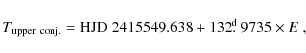
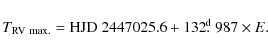
Results. We derived a new orbital ephemeris
![]() HJD (2447025.6
HJD (2447025.6![]() 1.8) + (132
1.8) + (132
![]() 987
987 ![]() 0
0
![]() 050)
050) ![]() .
The analysis of long-term spectral and light variations shows a clear correlation between the RV and V/R changes, and a very complex behaviour of the light changes. The character of the orbital light and V/R changes varies from season to season.
.
The analysis of long-term spectral and light variations shows a clear correlation between the RV and V/R changes, and a very complex behaviour of the light changes. The character of the orbital light and V/R changes varies from season to season.
Key words: stars: early-type - binaries: spectroscopic - stars: emission-line, Be - stars: individual: ![]() Tauri
Tauri
1 Introduction
In spite of strong efforts by several generations of observers and theoreticians, the very nature of the Be phenomenon and the causes of (mostly unpredictable) spectral and light variability of individual Be stars remain unexplained. This is obviously caused by the fact that Be stars vary on at least three distinct time scales - see, e.g. Harmanec (1983) - and these variations mutually interfere in a complex manner. Without really long and systematic series of spectral and photometric observations it is almost impossible to distinguish the variations on different time scales properly. This is why we believe that detailed studies of individual Be stars which have rich observational histories represent one important way to address this long-standing problem.
In this paper, we apply such an approach to the bright Be star
![]() Tau. The purpose of our study is manifold:
Tau. The purpose of our study is manifold:
- 1.
- To assemble all available spectroscopic, spectrophotometric,
photometric, and interferometric observations on Tau and to homogenize
them as much as possible. This is described in Sects. 2
and 3 and detailed in Appendixes A and B
of this paper. Those data will be published in a follow-up paper containing
the alternative model of long-term V/R changes.
- 2.
- To present the first truly comprehensive examination of the long-term variations in a Be star, identify the individual patterns, and examine the relationships between the spectroscopic and broad-band photometric changes (cf. Sect. 4).
- 3.
- To study the variations related to the binary nature of Tau.
To this end, we used (in Sect. 5) several different
techniques of data prewhitening for the long-term changes to provide
a convincing proof that the Be star with its envelope moves in a binary orbit
with an unseen secondary. We also derived an improved ephemeris and
the binary orbital elements and demonstrated a complex character of
the phase-locked light and V/R changes. By V/R we mean the ratio of
the intensities of violet
 and red
 emission peaks of double peaked emission lines measured in the units of
continuum level.
emission peaks of double peaked emission lines measured in the units of
continuum level.
Although quite extensive, our dataset is not suitable to a detailed study of rapid spectral and light changes since it contains only a very few whole-night series of observations or simultaneous observations from observatories with a large difference in local time. For that reason we plan to obtain new dedicated observations and postpone a detailed study of rapid changes for later.
The final conclusions of this paper are summarized in Sect. 7.
2 Relevant observational facts about Tau
The star ![]() Tau (HD 37202, 123 Tau, HR 1910, HIP 26451) is one of the brightest Be stars in the northern sky (V =2
Tau (HD 37202, 123 Tau, HR 1910, HIP 26451) is one of the brightest Be stars in the northern sky (V =2
![]() 7-3
7-3
![]() 2 var.), exhibiting spectral, brightness
and colour variations on several distinct time scales.
It is also a spectroscopic binary with an orbital period of 132
2 var.), exhibiting spectral, brightness
and colour variations on several distinct time scales.
It is also a spectroscopic binary with an orbital period of 132
![]() 97 days.
Its orbital radial-velocity (RV hereafter) variations are
superimposed on the cyclic long-term ones.
97 days.
Its orbital radial-velocity (RV hereafter) variations are
superimposed on the cyclic long-term ones. ![]() Tau also exhibits the
long-term V/R and emission-line strength changes.
Tau also exhibits the
long-term V/R and emission-line strength changes.
2.1 RV variations
The RV variations of ![]() Tau were first discovered by
Frost & Adams (1903), and Adams (1905) demonstrated that these
variations are periodic and concluded that
Tau were first discovered by
Frost & Adams (1903), and Adams (1905) demonstrated that these
variations are periodic and concluded that
![]() Tau is a spectroscopic binary with an orbital period
of 138 days. Losh (1932) improved the value of the period
to 133 days, but reported also long-term RV variations in addition to
the periodic ones. Since that time a large number of
spectroscopic studies of
Tau is a spectroscopic binary with an orbital period
of 138 days. Losh (1932) improved the value of the period
to 133 days, but reported also long-term RV variations in addition to
the periodic ones. Since that time a large number of
spectroscopic studies of ![]() Tau were carried out, for instance by
Hynek & Struve (1942), Underhill (1951,1952),
Miczaika (1953), Aydin et al. (1965),
Delplace (1970b,a), Abt & Levy (1978),
Harmanec (1984), Jarad (1987), Mon et al. (1992),
Guo et al. (1995), Rivinius et al. (2006), Pollmann & Rivinius (2008), and Stefl et al. (2009),
among others. Thanks to these studies it became clear that in certain
time intervals simple orbital RV changes are observed (with a full
amplitude of some 15 km s-1 ) while in others
cyclic long-term changes with variable cycle lengths (roughly between 4
and 7 years) and a full amplitude up to 150 km s-1 are superimposed on the orbital RV changes.
Tau were carried out, for instance by
Hynek & Struve (1942), Underhill (1951,1952),
Miczaika (1953), Aydin et al. (1965),
Delplace (1970b,a), Abt & Levy (1978),
Harmanec (1984), Jarad (1987), Mon et al. (1992),
Guo et al. (1995), Rivinius et al. (2006), Pollmann & Rivinius (2008), and Stefl et al. (2009),
among others. Thanks to these studies it became clear that in certain
time intervals simple orbital RV changes are observed (with a full
amplitude of some 15 km s-1 ) while in others
cyclic long-term changes with variable cycle lengths (roughly between 4
and 7 years) and a full amplitude up to 150 km s-1 are superimposed on the orbital RV changes.
Harmanec (1984) compiled all RVs available at that time, removed long-term
changes via spline functions, and derived the most accurate orbital ephemeris
which has then been adopted in the majority of consecutive studies. Harmanec (1984) and Floquet et al. (1989) concluded that
2.2 Spectral variations
Losh (1932) and Lockyer (1936) reported the presence of cyclic V/R variations on a time scale of several years as well as long-term line-strength changes.
Delplace (1970b) was probably the first one to point out that
the Balmer emission-line profiles are not always the usual double-peaked
emissions but can be more complicated - see her Fig. 6.
Depending on how one wants to interpret them, the profiles adopt
a shape of either three or even four distinct emission peaks or
emission with two or even three separate absorption cores.
Delplace (1970b) pointed out that these complicated profiles
appear only at specific phases of the long-term RV and V/R cycle.
Rivinius et al. (2006), Stefl et al. (2007), Pollmann & Rivinius (2008), and Stefl et al. (2009) confirmed the presence of such complicated H![]() line profiles in their electronic spectra. They argued that such profiles are observed when the V/R is close to one, but only on the rising branch of the V/R curve.
line profiles in their electronic spectra. They argued that such profiles are observed when the V/R is close to one, but only on the rising branch of the V/R curve.
2.3 Light and colour changes
Contrary to numerous spectroscopic observations, there are no systematic
photometric observations of ![]() Tau published before 1980. The first report about possible variability was by Köllnig-Schattschneider (1940) who observed
Tau published before 1980. The first report about possible variability was by Köllnig-Schattschneider (1940) who observed
![]() Tau during six nights in 1940. Haupt & Schroll (1974)
found a decrease in light of some 0
Tau during six nights in 1940. Haupt & Schroll (1974)
found a decrease in light of some 0
![]() 2 during 1968-1969.
Hubert-Delplace et al. (1982) were the first to note that a broad light minimum recorded
in the 13-colour system in the second half of the seventies
(Alvarez & Schuster 1981; Schuster & Alvarez 1983) coincides with the long-term V/R maximum
and also a RV maximum which was documented in detail by Hubert-Delplace et al. (1983).
The same correlation was also noted for another long-term cycle by
Vakili et al. (1998). First measurements in the
2 during 1968-1969.
Hubert-Delplace et al. (1982) were the first to note that a broad light minimum recorded
in the 13-colour system in the second half of the seventies
(Alvarez & Schuster 1981; Schuster & Alvarez 1983) coincides with the long-term V/R maximum
and also a RV maximum which was documented in detail by Hubert-Delplace et al. (1983).
The same correlation was also noted for another long-term cycle by
Vakili et al. (1998). First measurements in the ![]() system were secured at Hvar Observatory in the
winter of 1976/1977 and revealed a steady 0
system were secured at Hvar Observatory in the
winter of 1976/1977 and revealed a steady 0
![]() 1 decrease in V during the
observations.
1 decrease in V during the
observations.
A systematic monitoring of ![]() Tau at the Hvar Observatory started in 1981
and the first results were published by Pavlovski & Bozic (1982).
Bozic & Pavlovski (1988) classified the light variability of
Tau at the Hvar Observatory started in 1981
and the first results were published by Pavlovski & Bozic (1982).
Bozic & Pavlovski (1988) classified the light variability of ![]() Tau into three types:
Tau into three types:
- (1)
- long-term variations on the scale of years;
- (2)
- occasional orbital phase-locked light changes that were present in some cycles;
- (3)
- 0.8 day (or 1.6 day) rapid light variations with period and amplitude slightly varying in time.
The behaviour of the colour indices of ![]() Tau in time and in the
colour-colour diagram was briefly described by Pavlovski et al. (1997).
Both indices show variations of
Tau in time and in the
colour-colour diagram was briefly described by Pavlovski et al. (1997).
Both indices show variations of ![]() 0
0
![]() 1. In the (
1. In the (![]() )
vs. (
)
vs. (![]() )
diagram,
the colour variations of
)
diagram,
the colour variations of ![]() Tau correspond to an apparent transition
from the main sequence to the giant branch and back.
Tau correspond to an apparent transition
from the main sequence to the giant branch and back.
2.4 Interferometric observations
More recently, the star was observed with several optical interferometers which are capable of resolving the envelope around it (Vakili et al. 1998; Quirrenbach et al. 1997,1994). Using the Navy Prototype Optical Interferometer, Tycner et al. (2004) found that emission-line envelope which surrounds the primary star is well inside the Roche lobe around it. Gies et al. (2007) analyzed the most recent near-IR interferometric observations in the K band and concluded that the emission disk is viewed almost edge-on.
3 Observational material used
We compiled a large collection of radial velocities, spectrophotometric quantities and photometric observations for which dates of observations were available from the astronomical literature. Most of the RVs were previously compiled by Harmanec (1984), but we have critically revised these data and checked them with their original sources. In addition, we obtained and reduced a very large number of spectral and photometric observations ourselves. A detailed discussion of all observational data, their reduction and journals of observations are provided in Appendix A (spectroscopy) and B (photometry).
Here we only mention some important points relevant to further analyses.
Electronic spectra at our disposal mainly cover the red part of the
spectrum containing the Si II 6347 and 6371 'A doublet, H![]() and He I 6678 'A.
To be able to study both the orbital motion and the long-term changes
in the envelope, we measured RVs of the steep emission wings of H
and He I 6678 'A.
To be able to study both the orbital motion and the long-term changes
in the envelope, we measured RVs of the steep emission wings of H![]() ,
of the broad He I 6678 'A wings and also of the shell absorption cores of H
,
of the broad He I 6678 'A wings and also of the shell absorption cores of H![]() ,
He I 6678 'A, and the Si II 6347 and 6371 'A lines.
,
He I 6678 'A, and the Si II 6347 and 6371 'A lines.
Since ![]() Tau frequently displays a rather complicated H
Tau frequently displays a rather complicated H![]() profile
(Delplace 1970b; Rivinius et al. 2006), special attention was paid to the
determination of the V/R ratio of its emission peaks.
Besides ``ordinary'', double-peaked emission lines, in about 30% of
high-resolution spectra triple-peaked H
profile
(Delplace 1970b; Rivinius et al. 2006), special attention was paid to the
determination of the V/R ratio of its emission peaks.
Besides ``ordinary'', double-peaked emission lines, in about 30% of
high-resolution spectra triple-peaked H![]() profiles are seen
and on several occasions both emission peaks are divided in two
so the quadruple-peaked profiles are observed. This is probably due
to the presence of additional absorption components in the H
profiles are seen
and on several occasions both emission peaks are divided in two
so the quadruple-peaked profiles are observed. This is probably due
to the presence of additional absorption components in the H![]() line,
caused by complicated and possibly non-Keplerian kinematic structure
in the disc. In approximately 25% of the profiles the second absorption
component is seen, but no distinct third peak was formed and the
resulting double-peaked profile has one distinctly asymmetric peak (see
for instance the lowest profile in Fig. 1).
Sometimes, one sees a more or less central emission peak
and two fainter ones located on both sides from it.
In Fig. 1 a sequence of complicated profiles is shown.
A gradual transition from asymmetric, double-peaked profiles to
the triple-peaked ones and vice versa can be seen there. Such complicated
profiles make the determination of the V/R ratio difficult
or even meaningless.
line,
caused by complicated and possibly non-Keplerian kinematic structure
in the disc. In approximately 25% of the profiles the second absorption
component is seen, but no distinct third peak was formed and the
resulting double-peaked profile has one distinctly asymmetric peak (see
for instance the lowest profile in Fig. 1).
Sometimes, one sees a more or less central emission peak
and two fainter ones located on both sides from it.
In Fig. 1 a sequence of complicated profiles is shown.
A gradual transition from asymmetric, double-peaked profiles to
the triple-peaked ones and vice versa can be seen there. Such complicated
profiles make the determination of the V/R ratio difficult
or even meaningless.
![\begin{figure}
\par\includegraphics[width=7.5cm,clip]{10526f01.eps}
\end{figure}](/articles/aa/full_html/2009/42/aa10526-08/img26.png)
|
Figure 1:
Sequence of H |
| Open with DEXTER | |
To handle this problem, we split the dataset into two subsets,
according to the observed H![]() profile. One subset consists of simple
profiles by which we mean double-peaked profiles and/or profiles with
only one absorption core. The second subset contains complex profiles,
i.e., asymmetric double-peaked and multi-peaked profiles or profiles with
more than one absorption core.
profile. One subset consists of simple
profiles by which we mean double-peaked profiles and/or profiles with
only one absorption core. The second subset contains complex profiles,
i.e., asymmetric double-peaked and multi-peaked profiles or profiles with
more than one absorption core.
We measured peak and core intensities of all parts of the complicated profiles. To obtain an estimate of the V and R peak intensities and of the V/R
ratio, we derived the position of the centre of the whole emission
profile at an arbitrarily chosen intensity of 1.5 (in the units of
continuum level). We then averaged the measured intensities of all
peaks to the left of this centre
to obtain the value of V and to the right of it to obtain R and calculated
the V/R ratio from these estimates. Note that while some authors
use the notation V and R to denote the intensities of the emission
peaks only above the continuum level, our values are consistently
measured from zero intensity level![]() . We converted the data compiled from
the literature - if necessary - into our type of measurement.
Additionally, for complex profiles we measured RVs of
three separate absorption components: red, violet and central.
. We converted the data compiled from
the literature - if necessary - into our type of measurement.
Additionally, for complex profiles we measured RVs of
three separate absorption components: red, violet and central.
4 Long-term changes
![\begin{figure}
\par\includegraphics[width=9cm]{10526fb1.eps}\par\includegraphics...
...dth=9cm]{10526fb5.eps}\par\includegraphics[width=9cm]{10526fb6.eps}
\end{figure}](/articles/aa/full_html/2009/42/aa10526-08/img33.png)
|
Figure 2b: The same as Fig. 2a for the time interval HJD 2442000-2445750. |
![\begin{figure}
\par\includegraphics[width=9cm]{10526fc1.eps}\par\includegraphics...
...dth=9cm]{10526fc5.eps}\par\includegraphics[width=9cm]{10526fc6.eps}
\end{figure}](/articles/aa/full_html/2009/42/aa10526-08/img34.png)
|
Figure 2c: The same as Fig. 2a for the time interval HJD 2445750-2447750. |
![\begin{figure}
\par\includegraphics[width=9cm]{10526fd1.eps}\par\includegraphics...
...dth=9cm]{10526fd5.eps}\par\includegraphics[width=9cm]{10526fd6.eps}
\end{figure}](/articles/aa/full_html/2009/42/aa10526-08/img35.png)
|
Figure 2d: The same as Fig. 2a for the time interval HJD 2447750-2449750. |
![\begin{figure}
\par\includegraphics[width=9cm]{10526fe1.eps}\par\includegraphics...
...dth=9cm]{10526fe5.eps}\par\includegraphics[width=9cm]{10526fe6.eps}
\end{figure}](/articles/aa/full_html/2009/42/aa10526-08/img36.png)
|
Figure 2e: The same as Fig. 2a for the time interval HJD 2449750-2451750. |
![\begin{figure}
\par\includegraphics[width=8.88cm,clip]{10526ff1.eps}\par\include...
...{10526ff6.eps}\par\includegraphics[width=8.89cm,clip]{10526ff7.eps}
\end{figure}](/articles/aa/full_html/2009/42/aa10526-08/img37.png)
|
Figure 2f:
The same as Fig. 2a for the time
interval HJD 2451750-2454600. Additionally, the central intensity of the
H |
![\begin{figure}
\par\includegraphics[width=9cm]{10526f3a.eps}\par\includegraphics...
...dth=9cm]{10526f3d.eps}\par\includegraphics[width=9cm]{10526f3e.eps}
\end{figure}](/articles/aa/full_html/2009/42/aa10526-08/img38.png)
|
Figure 3:
Long-term variation of the H I shell RVs, the V/R ratio of the Balmer emission lines of |
| Open with DEXTER | |
A plot of various observables vs. time, based on individual data points, is shown in Figs. 2a-2f. It is obvious that all measured spectral and photometric quantities exhibit pronounced long-term variations but also variations on shorter time scales. The interpretation of long-term changes is by no means straightforward. The problem is that the long-term variations are affected by at least two independent processes: by long-term changes of the extent and density of the envelope (usually detected via the so-called E/C changes, i.e., changes in the ratio of intensity of the emission lines to the neighbouring continuum) and by the precession of an elongated non-axisymmetric envelope (which manifests itself by the V/R changes).
From Fig. 3, we see that over the last 100 years, ![]() Tau has gone
through three ``active'' stages characterized by pronounced long-term RV and V/R variations and two ``quiet'' stages in which the RV and V/R variations are less pronounced. During the active stages, the H
Tau has gone
through three ``active'' stages characterized by pronounced long-term RV and V/R variations and two ``quiet'' stages in which the RV and V/R variations are less pronounced. During the active stages, the H![]() emission tended to be
very strong, (i.e., it had a larger equivalent width); during quiet stages,
H
emission tended to be
very strong, (i.e., it had a larger equivalent width); during quiet stages,
H![]() emission profiles were less pronounced (cf., e.g., Figs. 2b
and 2c).
emission profiles were less pronounced (cf., e.g., Figs. 2b
and 2c).
Although the time coverage by different types of observations is less complete than what one would like to have, it seems from an inspection of Figs. 2a-2f that some patterns are emerging:
- 1.
- During all intervals when the long-term RV and V/R changes were present, they always vary in phase (Hubert-Delplace et al. 1983; Mon et al. 1992; Hubert et al. 1987).
- 2.
- Already Hubert-Delplace et al. (1982) and Vakili et al. (1998) noted that
the minimum brightness occurred near RV and V/R maxima on two
different occasions. It seems, however, that the behaviour is more
complex in fact. We note that during the time interval
JD 2436800-JD 2440500 also the EW varies in phase with the RV changes.
However, in the recent long-term cycles (
 ),
changes of the H
),
changes of the H EW are not in phase with the RV changes. Mennickent et al. (1997)
classified Tau as a star for which occultations of the stellar disk
by the density enhancement due to one-armed oscillation should be
observable on the descending branch of the long-term V/R cycles.
As Figs. 2a-2f show, the needed parallel V/R and
photometric data are missing. The only case where such a light decrease
could be suspected is the time interval around JD 2453600 but photometry
is very scarce there.
EW are not in phase with the RV changes. Mennickent et al. (1997)
classified Tau as a star for which occultations of the stellar disk
by the density enhancement due to one-armed oscillation should be
observable on the descending branch of the long-term V/R cycles.
As Figs. 2a-2f show, the needed parallel V/R and
photometric data are missing. The only case where such a light decrease
could be suspected is the time interval around JD 2453600 but photometry
is very scarce there.
- 3.
- The light variations are obviously quite complex and one can note
a rather frequent occurrence of sharp light decreases lasting
typically some 10-20 days. Notably, they are quite pronounced over
the time interval between HJD 2446000-2448000 when the long-term activity
more or less disappeared - see also Mon et al. (1992), Ballereau et al. (1992),
and Guo & Guo (1992) for the description of this interval without
long-term changes. The light decreases occur in different orbital phases of
the binary, not only during the binary conjunctions as originally
conjectured by Bozic & Pavlovski (1988). These light decreases are not accompanied
by any notable changes of the
 colour but are seen as a reddening in
  .
The only notable change of
colour is reddening up to 0
.
The only notable change of
colour is reddening up to 0
 1 around HJD 2450000
which takes place when the RV of the shell lines exceeds approximately 50 km s-1 for the first time since the beginning of new active phase.
1 around HJD 2450000
which takes place when the RV of the shell lines exceeds approximately 50 km s-1 for the first time since the beginning of new active phase.
- 4.
- The pattern of the long-term light changes
is less clear due to the fact that the light changes on shorter time scales
are quite pronounced. The general impression from the plot of V magnitude
shown in Fig. 3 is that the brightness of Tau
at the recorded brightness maxima
has been slowly increasing over the whole time interval of 44 years covered
by available photometry with known times of observations. Such an impression is
corroborated by the results of linear regression presented in Table 1.
The result for all available data, although not statistically
significant, shows that the brightness has been increasing during last
44 years. The results for several selected
subsets are somewhat confusing and indicate that both, the mild secular
decreases, as well as the large increase of EW in the period JD
2447750-2448750 are accompanied by the decrease
of the brightness.
- 5.
- The beginning of a new active phase more or less coincides with
the extensive use of electronic spectra and some correlations can be
studied in more detail - see Fig. 2f. As clearly seen in Fig. 3,
the complicated H
profiles with several absorption cores are
always only observed on the rising branch of the V/R cycle,
as first noted by Delplace (1970b) and Rivinius et al. (2006).
The increased accuracy of more recent data (shown in Fig. 2f)
allows us to conclude that the emission strength also exhibited some cyclic
changes during the last V/R cycle, attaining maximum when complex profiles are observed, i.e., in the middle of the rising branch of the V/R cycle.
Also, note that the depth of the H
shell core is lowest at the same time, i.e., the line intensity
measured from the zero level in the rectified spectra is maximum - see
panel
 in Fig. 2f.
It can be concluded that the complex profiles are observed when the
shell lines become weak and multiple, which contributes to the increase
of the equivalent width of the emission profile.
in Fig. 2f.
It can be concluded that the complex profiles are observed when the
shell lines become weak and multiple, which contributes to the increase
of the equivalent width of the emission profile.
Table 1:
Slopes obtained by linear regression (y=a x+b) for V magnitude and H![]() EW data for all available data and several subsets.
EW data for all available data and several subsets.
![\begin{figure}
\par\includegraphics[width=7cm]{10526f4a.eps}\par\includegraphics...
...th=7cm]{10526f4c.eps}\par\includegraphics[width=7cm]{10526f4d.eps}
\end{figure}](/articles/aa/full_html/2009/42/aa10526-08/img53.png)
|
Figure 4:
The ( |
| Open with DEXTER | |
The behaviour of ![]() Tau in the (
Tau in the (![]() )
vs. (
)
vs. (![]() )
diagram is shown in Fig. 4.
In the top panel, the data from the time interval HJD 2438306-2447630 are shown,
but the systematic observations started roughly round HJD 2445000. During this period
(HJD 2445000-2447630) there are no long term RV and V/R variations, i.e., the circumstellar disc is symmetrical and it is slowly dispersing.
Looking at Figs. 2b and 2c, it is evident that the
changes in
)
diagram is shown in Fig. 4.
In the top panel, the data from the time interval HJD 2438306-2447630 are shown,
but the systematic observations started roughly round HJD 2445000. During this period
(HJD 2445000-2447630) there are no long term RV and V/R variations, i.e., the circumstellar disc is symmetrical and it is slowly dispersing.
Looking at Figs. 2b and 2c, it is evident that the
changes in ![]() occur on short time scales. Those obviously reflect short-term
changes in the inner disk. Also, if the star is partially screened by the disc, the decreasing radius and/or density
of the disc will result in the increase of brightness and a tendency for
occur on short time scales. Those obviously reflect short-term
changes in the inner disk. Also, if the star is partially screened by the disc, the decreasing radius and/or density
of the disc will result in the increase of brightness and a tendency for ![]() and
and
![]() to become more blue due to a
decrease of absorption and scattering of the light in the disc.
On the other hand, the depletion of the disc will result in a decrease of emission from
the disc itself what will result in a brightness decrease, bluer
to become more blue due to a
decrease of absorption and scattering of the light in the disc.
On the other hand, the depletion of the disc will result in a decrease of emission from
the disc itself what will result in a brightness decrease, bluer ![]() and
redder
and
redder ![]() .
Therefore depletion of the disc results in
.
Therefore depletion of the disc results in ![]() changes while
changes while ![]() and brightness
remain roughly constant, and this is manifested in the colour-colour diagram as horizontal movement.
and brightness
remain roughly constant, and this is manifested in the colour-colour diagram as horizontal movement.
Around HJD 2448000 the H![]() EW reaches a minimum and starts to increase. This increase coincides
with the onset of the long-term RV and V/R
variations, i.e., the increasing density
and/or diameter of the disc coincides with development of an asymmetry
in the disc. The increase of emission is accompanied with a decrease of
brightness and redder
EW reaches a minimum and starts to increase. This increase coincides
with the onset of the long-term RV and V/R
variations, i.e., the increasing density
and/or diameter of the disc coincides with development of an asymmetry
in the disc. The increase of emission is accompanied with a decrease of
brightness and redder ![]() colour index (cf. Table 1 and Fig. 2d). This type of behaviour is typical for the inverse correlation between the H I emission strength and the luminosity
as defined by Harmanec (1983). However, no reddening of
colour index (cf. Table 1 and Fig. 2d). This type of behaviour is typical for the inverse correlation between the H I emission strength and the luminosity
as defined by Harmanec (1983). However, no reddening of ![]() is seen.
The effect is more pronounced due to the minimum of brightness and
is seen.
The effect is more pronounced due to the minimum of brightness and ![]() colour index which occurs immediately after the first maximum of the
long-term cycle (round HJD 2448500). This may be caused by the
transit of a newly formed density enhancement
in front of the star, i.e., when the densest part of asymmetrical disc
is projected to stellar surface. This minimum is denoted by empty
symbols in the second panel of Fig. 4.
colour index which occurs immediately after the first maximum of the
long-term cycle (round HJD 2448500). This may be caused by the
transit of a newly formed density enhancement
in front of the star, i.e., when the densest part of asymmetrical disc
is projected to stellar surface. This minimum is denoted by empty
symbols in the second panel of Fig. 4.
As already pointed out, the only notable change of the ![]() colour is
a reddening up to 0
colour is
a reddening up to 0
![]() 1 that occurred between HJD 2450000 and 2450100.
The change consists of few sharp reddenings which are accompanied by blueings of the
1 that occurred between HJD 2450000 and 2450100.
The change consists of few sharp reddenings which are accompanied by blueings of the ![]() colour and increases of brightness. This is a signature of the positive correlation as defined by Harmanec (1983). It is illustrated in the third panel of Fig. 4. Those changes take place when RV of the shell lines exceed some 50 km s-1 prior to maximum of long-term cycle, i.e., when newly formed density enhancement becomes visible after passing behind the star.
colour and increases of brightness. This is a signature of the positive correlation as defined by Harmanec (1983). It is illustrated in the third panel of Fig. 4. Those changes take place when RV of the shell lines exceed some 50 km s-1 prior to maximum of long-term cycle, i.e., when newly formed density enhancement becomes visible after passing behind the star.
In the remaining panel, the data from time interval HJD 2448897-2454131 are shown (with the data HJD 2450000-2450100 excluded there). It can be seen that the colour behaviour in this time interval is complex and reminiscent of a positive correlation.
It can be concluded that overall behaviour of ![]() Tau in the colour-colour diagram does not
consistently show either a positive or an inverse correlation between the H I emission strength and the luminosity. This kind of behaviour is typical for stars with intermediate inclination,
where the inhomogeneous structure of the disc and changing rate of screening will disturb the simple correlation between the H I emission strength and the luminosity; see, e.g.,
Tau in the colour-colour diagram does not
consistently show either a positive or an inverse correlation between the H I emission strength and the luminosity. This kind of behaviour is typical for stars with intermediate inclination,
where the inhomogeneous structure of the disc and changing rate of screening will disturb the simple correlation between the H I emission strength and the luminosity; see, e.g., ![]() Dra (Juza et al. 1994) and 4 Her (Koubský et al. 1997). On the other hand, the estimated inclination of
Dra (Juza et al. 1994) and 4 Her (Koubský et al. 1997). On the other hand, the estimated inclination of ![]() Tau is in the range of 67
Tau is in the range of 67![]() to 87
to 87![]() ,
too high to support this picture.
,
too high to support this picture.
5 Orbital changes
5.1 RV changes, orbital solutions and a new ephemeris
The determination of reliable orbital RV curves of Be stars which are members of binary systems is difficult due to presence of variations on several different timescales. This is reflected in the determination of their correct orbital elements.
The RV curves based on the sharp shell absorption lines are often affected by asymmetries
which result in RV curves with sharp maxima and flat minima, reminiscent
of eccentric orbits with the longitude of periastron near ![]() - see,
e.g., Fig. 3 in Harmanec (1985), for numerous examples of such curves.
The RV curves of the rotationally broadened He I lines, supposed to originate in the stellar photosphere - or at least
in the densest inner parts of the envelope close to the true photosphere -
usually show a very large scatter around the mean RV curve.
This additional scatter is probably caused by the rapid line-profile
variations. Harmanec et al. (2002b) argued that the RV curves of Be star binaries, based on
He I line profiles, might be affected by the phase-locked V/R changes,
and that this may lead to the overestimation of the orbital semi-amplitudes.
That this is indeed the case for several studied Be binaries
(
- see,
e.g., Fig. 3 in Harmanec (1985), for numerous examples of such curves.
The RV curves of the rotationally broadened He I lines, supposed to originate in the stellar photosphere - or at least
in the densest inner parts of the envelope close to the true photosphere -
usually show a very large scatter around the mean RV curve.
This additional scatter is probably caused by the rapid line-profile
variations. Harmanec et al. (2002b) argued that the RV curves of Be star binaries, based on
He I line profiles, might be affected by the phase-locked V/R changes,
and that this may lead to the overestimation of the orbital semi-amplitudes.
That this is indeed the case for several studied Be binaries
(![]() Cas,
Cas, ![]() Per,
Per, ![]() Dra, V839 Her and V832 Cyg)
was shown in Harmanec (2003).
Dra, V839 Her and V832 Cyg)
was shown in Harmanec (2003).
Following Bozic et al. (1995), we measured the steep wings of the strong
H![]() emission to obtain the most realistic estimate of the
orbital motion of the B primary. This approach led to the determination of
orbital RV curves for several other Be binaries (see Harmanec (2003)
and references therein). The reasons why it should be so are the
following:
emission to obtain the most realistic estimate of the
orbital motion of the B primary. This approach led to the determination of
orbital RV curves for several other Be binaries (see Harmanec (2003)
and references therein). The reasons why it should be so are the
following:
- 1.
- any available models of the disks indicate that their outer parts rotate more slowly than their inner parts;
- 2.
- it is very probable that at least the denser inner parts of the disk in a binary system will adopt the shape of corresponding equipotential surfaces of the Roche model. It is easy to see that inside the critical Roche lobe these equipotentials quickly become almost spherical;
- 3.
- the two previous facts imply that while the peaks of the H
emission can be affected by asymmetries of
the outer part of the disk, the steep wings reflect the motion
of the roughly symmetric inner parts of the disk;
- 4.
- thanks to high density of the inner parts, the scattering wings
of H
are roughly insensitive to geometry;
- 5.
- any asymmetry in the gas distribution of the inner disk is likely to circularize in a few orbital periods due to viscous effects.
The time coverage of the available spectra is less uniform than that required
for reliable removal of the long-term trend. We attempted to remove the long-term RV
variations using the program HEC13 based on a fit via spline functions after
Vondrák (1977,1969)![]() .
After a few experiments, as the optimal choice we used the smoothing parameter
.
After a few experiments, as the optimal choice we used the smoothing parameter
![]() through the 5-day moving box-car averaged RV points. The time plot of the H
through the 5-day moving box-car averaged RV points. The time plot of the H![]() emission-wing RVs and the spline fit used are shown in Fig. 5. Note that we defined the spline function using
RVs from both the electronic spectra and from digitized Ondrejov photographic spectrograms.
emission-wing RVs and the spline fit used are shown in Fig. 5. Note that we defined the spline function using
RVs from both the electronic spectra and from digitized Ondrejov photographic spectrograms.
| Figure 5:
The time plot of all RVs of the H |
|
| Open with DEXTER | |
To check how the RVs were prewhitened for the long-term changes, we
divided them into subsets spanning not more than some 600 days and
derived another RV solution in which different ``systemic velocities''
were allowed for individual subsets. We omitted a few single RVs which
could not be combined into a subset
with a sufficient phase coverage. This way, we also allowed for the
removal of
the long-term RV changes. The resulting RV curve is compared to that
based
on the residuals from the spline function in Fig. 6 and both
trial solutions are compared as solutions 1 and 2 in Table 2.
Although the two phase curves in Fig. 6 are not identical,
their similarity is obvious and proves the reality of the orbital motion.
Moreover, the semiamplitudes of both curves, based on the
orbital solutions with the latest publicly available version of the
program FOTEL (Hadrava 2004,1990), are comparable, 6.5 ![]() 0.5 km s-1, and 7.4
0.5 km s-1, and 7.4 ![]() 0.5 km s-1. RVs from the digitized photographic spectra have actually
only slightly higher rms errors than those from the electronic ones
(5.5 vs. 4.6 km s-1).
0.5 km s-1. RVs from the digitized photographic spectra have actually
only slightly higher rms errors than those from the electronic ones
(5.5 vs. 4.6 km s-1).
![\begin{figure}
\par\includegraphics[angle=-90,width=8cm,clip]{10526f6a.eps}
\includegraphics[angle=-90,width=8cm,clip]{10526f6b.eps}
\end{figure}](/articles/aa/full_html/2009/42/aa10526-08/img60.png)
|
Figure 6:
The orbital RV curve of the H |
| Open with DEXTER | |
As the next step, we re-investigated also all published RVs based on
the H I and He I lines. It is a difficult task to use these RVs
to improve the value of the orbital period since in the majority
of cases these RVs are affected by the contribution of circumstellar shell
and its long-term changes. Note also that the RV curve of more accurately
measured H I shell lines is distorted, having a sharp maximum and
a bump near the RV minimum (see Fig. 7).
Those bumps were interpreted by Harmanec (1985)
as a influence of a gas stream flowing from the secondary, projected in
the certain orbital phases against the primary. In the global
oscillation scenario, the disc dynamics is modified when the one-armed
spiral pattern forms and important radial components appear (see Okazaki 1997,
for instance).
It is conceivable that the disturbance pattern in the outer
parts of the disc is responsible for the observed distortions of the RV
curve and the appearance of the bump. The problem is that in the case
of ![]() Tau the bump is present also in the periods without long-term variations (see Fig. 3 in Harmanec 1985).
Anyhow, it is not quite clear if it is legitimate to compare the RV
maxima of such distorted curves with the RV maximum of the sinusoidal
RV curve based on the H
Tau the bump is present also in the periods without long-term variations (see Fig. 3 in Harmanec 1985).
Anyhow, it is not quite clear if it is legitimate to compare the RV
maxima of such distorted curves with the RV maximum of the sinusoidal
RV curve based on the H![]() emission wings.
emission wings.
In Table 3 we present three other solutions (denoted 3-5).
Solution 3 is based on all H I shell RVs measured on blue
photographic spectra and prewhitened for long-term changes with
HEC13 (
![]() ,
5-d normals), solution 4 is
based on He I RVs from photographic spectra combined with
He I 6678 core RVs from electronic spectra (prewhitened
with
,
5-d normals), solution 4 is
based on He I RVs from photographic spectra combined with
He I 6678 core RVs from electronic spectra (prewhitened
with
![]() ,
5-d normals). Solution 5 is
based on a combination of H
,
5-d normals). Solution 5 is
based on a combination of H![]() emission-wing RVs (different systemic
velocities for less than 600-d long subgroups as in solution 2 were allowed)
combined with He I RVs derived via cross-correlation by Jarad (1987).
emission-wing RVs (different systemic
velocities for less than 600-d long subgroups as in solution 2 were allowed)
combined with He I RVs derived via cross-correlation by Jarad (1987).
Table 2:
Trial circular-orbit solutions for the RVs measured on the H![]() emission wings.
emission wings.
Table 3:
Trial solutions for the H I shell RVs,
He I RVs and a combination of H![]() emission-wing RVs with He I
RVs measured via cross-correlation in Jarad (1987).
emission-wing RVs with He I
RVs measured via cross-correlation in Jarad (1987).
The results are somewhat confusing and we note that the different
solutions for the orbital period in solutions 1-5 are very
similar,
so the specific choice is not critical for the long-term variations.
The interval spanned by the RV observations
JD 2415794-JD 2454490, represents 290.95 cycles for the
period of 133
![]() 0, and 291.17 cycles for 132
0, and 291.17 cycles for 132
![]() 9.
The difference can be caused by the changes in the circumstellar
matter. This is illustrated by Fig. 7 where a gradual
development of a secondary RV maximum near the bottom of the RV curve
is seen. We therefore conclude that solution 2 of Table 2
represents the best currently available solution and we shall adopt it
to define the final binary ephemeris to be used in the rest of this
study:
9.
The difference can be caused by the changes in the circumstellar
matter. This is illustrated by Fig. 7 where a gradual
development of a secondary RV maximum near the bottom of the RV curve
is seen. We therefore conclude that solution 2 of Table 2
represents the best currently available solution and we shall adopt it
to define the final binary ephemeris to be used in the rest of this
study:
Recall that solution 2 is based on the prewhitening based on locally derived shifts of the systemic velocity which is a safer procedure for data with gaps than a somewhat subjective prewhitening via the spline functions. In any case, the difference between the two solutions is not critical for any practical purposes. Comparison of the ephemeris (2) and (1) reveals that the errors of the period and epoch were somewhat underestimated in Harmanec (1984).
Also, we would like to mention that for complex H![]() profiles we
measured RVs of three distinct absorption cores.
We found that all three are involved in the orbital motion and are, therefore,
true absorption lines, not ``holes'' between two neighbouring emission peaks.
The middle core (shown in Fig. 7) displays the most distorted
RV curve, reminiscent of the one based on the blue H I shell lines but
with more noise, perhaps due to blending with telluric lines and poor
visibility inside the strong emission.
profiles we
measured RVs of three distinct absorption cores.
We found that all three are involved in the orbital motion and are, therefore,
true absorption lines, not ``holes'' between two neighbouring emission peaks.
The middle core (shown in Fig. 7) displays the most distorted
RV curve, reminiscent of the one based on the blue H I shell lines but
with more noise, perhaps due to blending with telluric lines and poor
visibility inside the strong emission.
Adopting tentatively K = 7 km s-1 and M1 = 11 ![]() ,
we estimated the basic
properties of the binary. They are summarized in Table 4
for several plausible values of the orbital inclination.
,
we estimated the basic
properties of the binary. They are summarized in Table 4
for several plausible values of the orbital inclination.
![\begin{figure}
\par\includegraphics[width=8.8cm]{10526f7a.eps}\par\includegraphi...
...10526f7d.eps}\\ [2.5mm]
\includegraphics[width=8.8cm]{10526f7e.eps}
\end{figure}](/articles/aa/full_html/2009/42/aa10526-08/img68.png)
|
Figure 7:
Phase plot of several subsets of H I shell RVs, prewhitened for the long-term changes, vs. orbital phase. One can see
the gradual development of the bump near the minimum RV. In the bottom panel, the RVs of the H |
| Open with DEXTER | |
In spite of various uncertainties in the basic physical properties
of the Be primary, it is clear that the secondary is a low-mass object.
It could be a hot subdwarf like the secondary of ![]() Per (Gies et al. 1998).
However, in contrast to that binary, we have not detected any sharp
emission in the He I 6678 'A line which would moving in antiphase
to the RV curve of the Be star. Note that according to Hummel & Stefl (2001),
such an emission originates in a part of the Be-star disk, facing the
hot secondary, which is illuminated by it. Alternatively, the secondary
of
Per (Gies et al. 1998).
However, in contrast to that binary, we have not detected any sharp
emission in the He I 6678 'A line which would moving in antiphase
to the RV curve of the Be star. Note that according to Hummel & Stefl (2001),
such an emission originates in a part of the Be-star disk, facing the
hot secondary, which is illuminated by it. Alternatively, the secondary
of ![]() Tau can also be a normal solar-like main-sequence star.
In any case, the direct detection of the secondary will be very difficult.
Tau can also be a normal solar-like main-sequence star.
In any case, the direct detection of the secondary will be very difficult.
5.2 Spectrophotometric and photometric orbital phase-locked changes
Contrary to the RV changes, possible orbital phase-locked variations of
other observables were not frequently studied in the past.
Pavlovski & Bozic (1982) reported occasional decreases of brightness in the season
1981/82 which coincided almost exactly with the moment of the expected
superior conjunctions based upon the Harmanec (1984) ephemeris as shown
by Bozic & Pavlovski (1988). Most recently Pollmann & Rivinius (2008) found a
![]() d cycle in V/R variations between JD 2452100 and JD 2453500.
d cycle in V/R variations between JD 2452100 and JD 2453500.
Table 4:
Basic properties of the binary system estimated for
K=7 km s-1 and M1=11 ![]() and for several plausible orbital inclinations.
and for several plausible orbital inclinations.
![\begin{figure}
\par\includegraphics[width=8.8cm]{10526f08.eps}
\end{figure}](/articles/aa/full_html/2009/42/aa10526-08/img73.png)
|
Figure 8: Stelingwerf's PDM periodogram of the V/R ratio prewhitened for the long-term changes using spline functions. Solid line shows the analysis of simple double-peaked profiles, the dashed line the triple-peaked profiles. The arrow denotes the frequency of the orbital period. |
| Open with DEXTER | |
![\begin{figure}
\par\mbox{\includegraphics[angle=-90,scale=0.42]{10526f9a.ps}\inc...
...{10526f9c.ps}\includegraphics[angle=-90,scale=0.42]{10526f9d.ps} }\end{figure}](/articles/aa/full_html/2009/42/aa10526-08/img74.png)
|
Figure 9: Phase plots of individual V/R ( upper row) and V magnitude ( lower row) observations. Ephemeris from solution 2 are used and long-term changes were removed using Hermite polynomial interpolation scheme. Left: HJD < 2449000 subset. Right: HJD > 2449000 subset. |
| Open with DEXTER | |
To investigate the orbital modulation of emission lines and light variations
the H![]() EW and V/R, He I 6678 'A EW and intensity, V magnitude,
EW and V/R, He I 6678 'A EW and intensity, V magnitude,
![]() and
and ![]() colours were analysed. The long-term variations were removed
using HEC13, and a search for periodicity in the range of periods from 10 to 2000 days was performed using PDM (Stellingwerf 1978).
The analysis was done for the whole data set, and separately for two
subsets resulting from the division of the data near HJD 2449000.
With the exception of the V/R ratio, there are no peaks in the periodograms above
the noise level at a frequency corresponding to the orbital period.
For the V/R ratio, we analysed also the profiles of different complexities
separately. It was found that complex profiles show orbital variations while
the simple double-peaked profiles show weak or no orbital variation at all.
This is illustrated in Fig. 8 where the PDM periodograms
of the V/R ratio for double-peaked and more complex H
colours were analysed. The long-term variations were removed
using HEC13, and a search for periodicity in the range of periods from 10 to 2000 days was performed using PDM (Stellingwerf 1978).
The analysis was done for the whole data set, and separately for two
subsets resulting from the division of the data near HJD 2449000.
With the exception of the V/R ratio, there are no peaks in the periodograms above
the noise level at a frequency corresponding to the orbital period.
For the V/R ratio, we analysed also the profiles of different complexities
separately. It was found that complex profiles show orbital variations while
the simple double-peaked profiles show weak or no orbital variation at all.
This is illustrated in Fig. 8 where the PDM periodograms
of the V/R ratio for double-peaked and more complex H![]() profiles are
displayed. For simple profiles, the PDM analysis yields a period of
69
profiles are
displayed. For simple profiles, the PDM analysis yields a period of
69
![]() 6. The PDM analysis of all profiles (regardless of complexity) observed before
JD 2449000 (HJD < 2449000 subset) gives 66
6. The PDM analysis of all profiles (regardless of complexity) observed before
JD 2449000 (HJD < 2449000 subset) gives 66
![]() 5, or 133
5, or 133
![]() 0
with a double-wave curve, and the analysis of all profiles obtained after
this date (HJD > 2449000 subset) yields 69
0
with a double-wave curve, and the analysis of all profiles obtained after
this date (HJD > 2449000 subset) yields 69
![]() 6 or 139
6 or 139
![]() 1 with a double-wave curve. If complicated profiles are excluded those results do not change significantly.
1 with a double-wave curve. If complicated profiles are excluded those results do not change significantly.
To check the above-mentioned results, we prewhitened alternatively
the V magnitude and V/R data for the long-term changes using
the program HEC36 which is based on the Hermite polynomial
interpolation scheme as provided in the program INTEP by Hill (1982)![]() .
The residuals were then analysed using PERIOD04 (Lenz & Breger 2005).
The whole data set as well as HJD < 2449000 and HJD > 2449000 subsets were
analysed and simple and complex profiles were treated together.
The analysis of the V magnitude data yields several periods
in the range 50 to 200 days, while the analysis of V/R data gave similar periods as PDM. Analysis of the complete V/R dataset finds 69
.
The residuals were then analysed using PERIOD04 (Lenz & Breger 2005).
The whole data set as well as HJD < 2449000 and HJD > 2449000 subsets were
analysed and simple and complex profiles were treated together.
The analysis of the V magnitude data yields several periods
in the range 50 to 200 days, while the analysis of V/R data gave similar periods as PDM. Analysis of the complete V/R dataset finds 69
![]() 2 as the best period, the HJD > 2449000 subset gives both 69
2 as the best period, the HJD > 2449000 subset gives both 69
![]() 5, and 66
5, and 66
![]() 5
periods, while
the analysis of HJD < 2449000 subset does not yield any
period in the vicinity of orbital period or in the range
60-70 days.
5
periods, while
the analysis of HJD < 2449000 subset does not yield any
period in the vicinity of orbital period or in the range
60-70 days.
Orbital phase plots for the V magnitude and V/R ratio, based on individual data points, are shown in Fig. 9. Some orbital modulation of both studied quantities is seen there. To examine the orbital modulation in more detail, the observations were divided into individual observing seasons. For the V/R ratio, only the HJD > 2449000 subset was analysed.
Upon examination of orbital phase plots for individual observing seasons it can be concluded that the orbital light and V/R curves are changing from season to season, both in amplitude and phase. The amplitude of the V/R variation is smaller near the minimum, and larger near the maximum of the long-term RV cycle - see Fig. 10. Due to the relatively small number of measurements during any one season it is difficult to draw conclusions about the changes in phase. The changes in orbital light modulation are more complicated and there is no obvious connection to the long-term cycle. This is a consequence of light decreases that occur at arbitrary orbital phases and of rapid variations of brightness.
![\begin{figure}
\par\mbox{\includegraphics[angle=-90,scale=0.32]{1052610a.ps}\inc...
...ncludegraphics[angle=-90,scale=0.32]{1052610f.ps} }\vspace*{4mm}
\end{figure}](/articles/aa/full_html/2009/42/aa10526-08/img75.png)
|
Figure 10: Orbital phase plots of individual V observations ( left panels) and the V/R ratio ( central and right panels) for individual observing seasons. Seasons with larger amplitude of orbital variations (HJD 2450726-2450918, 2451237-2451572 and 2453231-2453482 from left to right) are shown in the upper row, and the seasons with smaller amplitude of orbital variations (HJD 2451075-2451278, 2451850-2452002 and 2453611-2453844) are plotted in the lower row. |
| Open with DEXTER | |
The period analysis of V/R data revealed the period of 69.6 or
a twice longer 139.1-d period exhibiting a double wave phase curve.
(We note that Adams (1905) derived a period of 138 days as the best one
for the RV variations from the first observed quiet period without
long-term changes but the relevance of this coincidence is not clear).
Note, however, that the following relation between the orbital and 139.1-d
period holds:
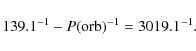
Note that the 3019-d ``period'' is the value comparable to the length of the long-term cyclic change during the last cycles covered by electronic spectra. It is conceivable, then, that the V/R ratio is actually modulated simultaneously by the orbital period and by cyclic long-term changes while the 69/139-d period is an apparent period only, resulting from the beat of the former two.
Another possible explanation of the 69
![]() 6
period could be a temporal presence of a blob of material in a
Keplerian orbit around the primary, not very far from its Roche lobe.
For instance, a blob orbiting around an 11
6
period could be a temporal presence of a blob of material in a
Keplerian orbit around the primary, not very far from its Roche lobe.
For instance, a blob orbiting around an 11 ![]() primary with a period of 69.6 days, would be located at an effective distance of 106
primary with a period of 69.6 days, would be located at an effective distance of 106 ![]() .
For the RV semi-amplitude of the primary K1=7.0 km s-1, the radius of the Roche lobe around the primary is larger than 150
.
For the RV semi-amplitude of the primary K1=7.0 km s-1, the radius of the Roche lobe around the primary is larger than 150 ![]() for any orbital inclination between 60
for any orbital inclination between 60![]() and 90
and 90![]() - see Table 4.
- see Table 4.
6 Towards physical interpretation of long-term changes
As it was shown in the previous sections, ![]() Tau is a very intricate
object. In the past, there were several attempts to understand the
physical nature of the long-term changes. Struve (1931) suggested that the cyclic long-term RV and V/R
variations of some Be stars could be explained if the circumstellar
disk temporarily adopts an elongated (elliptical) shape and slowly
revolves around the star. Johnson (1958) was the
first who pointed out that such a revolution of an elliptical envelope
is a direct analogy to the binary apsidal motion caused by the mass
distribution inside the star. He argued that the apsidal period of the
elongated envelope
Tau is a very intricate
object. In the past, there were several attempts to understand the
physical nature of the long-term changes. Struve (1931) suggested that the cyclic long-term RV and V/R
variations of some Be stars could be explained if the circumstellar
disk temporarily adopts an elongated (elliptical) shape and slowly
revolves around the star. Johnson (1958) was the
first who pointed out that such a revolution of an elliptical envelope
is a direct analogy to the binary apsidal motion caused by the mass
distribution inside the star. He argued that the apsidal period of the
elongated envelope
![]() can be calculated as
can be calculated as
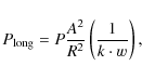
where P is the orbital period of the particles in the elliptical envelope, A the mean distance of the disk particles from the centre of the star, R the stellar radius, k the usual constant of internal structure of the star, and w is the ratio of centrifugal to gravitational force. Using values typical for Be stars, he found that formula (4) gives periods of the order of several years as observed. McLaughlin (1961) indeed showed for a simple geometrical model of a thin elliptical envelope that a slow revolution of such a structure leads to parallel RV and V/R variations of emission lines and RV variations of the shell absorption lines, in agreement with available observations. Kríz & Harmanec (1975) pointed out that an elongated envelope could be formed by a short-living inflow of material towards the Be star from its binary companion. They found from particle-trajectory calculations that such an envelope would revolve thanks to the attractive force of the binary component even around a point-like star, i.e., without the effect of the classical apsidal motion. In recent years, the most popular explanation of the long-term spectral changes of Be stars has been that the apparent asymmetry of the disk is a one-armed oscillation pattern as suggested by Kato (1983). The wide acceptance of Kato's model stems from the fact that it was quantitatively developed in a number of studies - for instance by Okazaki (1991), Okazaki (1996), Okazaki (1997), Papaloizou et al. (1992), Papaloizou & Savonije (2006), Firt & Harmanec (2006), Ogilvie (2008) and Carciofi et al. (2009) among others. In those studies, two different effects were considered (alternately and together) to maintain the oscillations: (1) the force of the radiative pressure gradient, and (2) the quadrupole term of the gravitational potential that arises from rotational flattening; see Johnson (1958). Ogilvie (2008) used a 3-D modelling of the oscillation and concluded that the 3-D effects are substantial and lead to the observed prograde rotation of the density enhancement (Vakili et al. 1998) even if the radiative force is neglected and the quadrupole mode of the gravitational potential is negligible.
In contrast to the above-mentioned studies which simply postulate
the existence of a circumstellar disk around a single star and study its
perturbations, Kríz & Harmanec (1975) tried the explain the very origin and
time evolution of the disk via a model of a discontinuous mass transfer
from a secondary star in a binary system. It is true that their model
postulated a Roche-lobe filling secondary and no such a large cool
secondary was detected - see, e.g., Floquet et al. (1989).
However,
their idea of putting a blob of material into an orbit around
a rapidly rotating B star is more general. First, such inflow of
material could occur in the form of a density enhancement in the
stellar wind from a very hot O subdwarf secondary (like the
secondary of a similar Be system ![]() Per), or in the form of coronal mass ejections from a solar-like, chromospherically active secondary. Note also that Harmanec et al. (2002a)
showed that even if the gas forming the Be envelope is outflowing from
the rapidly rotating B star which is a member of a binary without
any mass transfer, the outflow will not occur from the whole stellar
equator but only from the rotational Lagrangian point L1 facing
the secondary. They also demonstrated via 3-D gasdynamical modelling that
this can lead to the formation of an envelope around the B star.
Per), or in the form of coronal mass ejections from a solar-like, chromospherically active secondary. Note also that Harmanec et al. (2002a)
showed that even if the gas forming the Be envelope is outflowing from
the rapidly rotating B star which is a member of a binary without
any mass transfer, the outflow will not occur from the whole stellar
equator but only from the rotational Lagrangian point L1 facing
the secondary. They also demonstrated via 3-D gasdynamical modelling that
this can lead to the formation of an envelope around the B star.
Unfortunately, no quantitative modelling as that carried out
for one-armed oscillation model has been performed for the alternative idea of Kríz & Harmanec (1975). Since the binary character of ![]() Tau
is
rather firmly established, we consider a quantitative investigation of
their scenario to be important and intend to present our first effort
along this direction in a follow-up study.
Tau
is
rather firmly established, we consider a quantitative investigation of
their scenario to be important and intend to present our first effort
along this direction in a follow-up study.
To inspire future observational effort, we emphasize that both alternative models would make definite predictions for polarization changes, and that time variable polarization would need to be analysed in conjunction with the spectral data in order to fully test possible options.
7 Conclusions
Thanks to rich series of new spectroscopic, spectrophotometric, photometric
and interferometric observations and to a critical compilation of published
observational data it was possible to document the pattern of
the variations of ![]() Tau on several distinct time scales.
Tau on several distinct time scales.
Our principal results are summarized below:
- 1.
- During the last 100 years Tau has gone through three active stages with
pronounced long-term variations and two quiet stages. We found that
the time intervals when pronounced long-term variations occur coincide with
the presence of a strong Balmer emission and that they cease with the decrease
of its strength. During the intervals of the long-term activity,
RV and V/R variations are in phase, while the brightness and the emission
strength display more complex behaviour, obviously partly affected also by
changes on shorter time scales. The apparent correlation between
the brightness and emission strength changes in time.
- 2.
- More complicated H
profiles, with additional blue- and red-shifted
absorption components (which all share the orbital motion of the Be primary)
are always observed on the rising branch of the long-term V/R cycles
when the shell lines become weak and the emission becomes consequently
stronger.
- 3.
- Measuring the RVs on the steep wings of the H
emission and utilizing
different techniques of data prewhitening, we provided a rather firm proof
that the Be star Tau is indeed the primary component of a binary system
with an essentially circular 133-d orbit and a semiamplitude of
 km s-1. We derived an improved binary ephemeris.
- 4.
- We discovered mild and complicated phase-locked V/R and brightness variations and demonstrated that they change from season to season. The amplitude of the orbital V/R variations was found to attain a maximum and minimum near the maxima and minima of the long-term cycles, respectively.
D. Ruzdjak acknowledges the possibility to digitize the Ondrejov photographic spectra with the microdensitometer of the Astronomical Institute of the Slovak Academy of Sciences at Stará Lesná, help and hospitality provided by Dr. J. Zverko, V. Kollár, Dr. R. Komzík and Dr. M. Vanko there. We thank Dr. S. Ilovaisky who provided us with accurate mid-exposure times for the Observatoire de Haute Provence photographic spectra studied by Dr. Hubert-Delplace. She kindly helped us to resolve some larger differences in the dates of her plates and the list provided by Dr. Ilovaisky. We are also obliged to Drs. G. Burki, H. F. Haupt, J. Paparo, J. R. Percy, and A. Schroll, and Messrs. C. Buil, M. Muminovic and M. Stupar who provided us with their unpublished individual observations of
References
- Abt, H. A., & Levy, S. G. 1978, ApJS, 36, 241 [NASA ADS] [CrossRef]
- Adams, W. S. 1905, ApJ, 22, 115 [NASA ADS] [CrossRef]
- Alvarez, M., & Schuster, W. J. 1981, Rev. Mex. Astron. Astrofis., 6, 6, 163
- Andrillat, Y., & Fehrenbach, C. 1982, A&AS, 48, 93 [NASA ADS]
- Aydin, C., Hack, M., & Islik, S. 1965, Mem. Soc. Astron. Ital., 36, 331 [NASA ADS]
- Ballereau, D., Alvarez, M., Chauville, J., et al. 1987, Rev. Mex. Astron. Astrofis., 15, 29 [NASA ADS]
- Ballereau, D., Chauville, J., Hubert, A. M., et al. 1992, IAU Circ., 5539, 1
- Banerjee, D. P. K., Rawat, S. D., & Janardhan, P. 2000, A&AS, 147, 229 [NASA ADS] [CrossRef] [EDP Sciences]
- Bossi, M., & Guerrero, G. 1989, Informational Bulletin on Variable Stars, 3326, 1
- Bozic, H., & Pavlovski, K. 1988, Hvar Observatory Bulletin, 12, 15 [NASA ADS]
- Bozic, H., Harmanec, P., Horn, J., et al. 1995, A&A, 304, 235 [NASA ADS]
- Carciofi, A. C., Okazaki, A. T., le Bouquin, J., et al. 2009, A&A, 504, 915 [CrossRef] [EDP Sciences]
- Dachs, J., Hummel, W., & Hanuschik, R. W. 1992, A&AS, 95, 437 [NASA ADS]
- Delplace, A. M. 1970a, A&A, 7, 68 [NASA ADS]
- Delplace, A. M. 1970b, A&A, 7, 459 [NASA ADS]
- Firt, R., & Harmanec, P. 2006, A&A, 447, 277 [NASA ADS] [CrossRef] [EDP Sciences]
- Floquet, M., Hubert, A. M., Chauville, J., Chatzichristou, H., & Maillard, J. P. 1989, A&A, 214, 295 [NASA ADS]
- Frost, E. B., & Adams, W. S. 1903, ApJ, 17, 150 [NASA ADS] [CrossRef]
- Galkina, T. S. 1985, Izv. Krymskoj Astrofizicheskoj Observatorii, 72, 72 [NASA ADS]
- Gies, D. R., Bagnuolo, Jr., W. G., Ferrara, E. C., et al. 1998, ApJ, 493, 440 [NASA ADS] [CrossRef]
- Gies, D. R., Bagnuolo, Jr., W. G., Baines, E. K., et al. 2007, ApJ, 654, 527 [NASA ADS] [CrossRef]
- Gökgöz, A., Hack, M., & Kendir, I. 1962, Mem. Soc. Astron. Ital., 33, 239 [NASA ADS]
- Gögköz, A., Hack, M., & Kendir, I. 1963, Mem. Soc. Astron. Ital., 34, 87 [NASA ADS]
- Guo, Y. 1994, Informational Bulletin on Variable Stars, 4112, 1
- Guo, Y., & Guo, X. 1992, Informational Bulletin on Variable Stars, 3786, 1
- Guo, Y., Huang, L., Hao, J., et al. 1995, A&AS, 112, 201 [NASA ADS]
- Hadrava, P. 1990, Contributions of the Astronomical Observatory Skalnaté Pleso, 20, 23 [NASA ADS]
- Hadrava, P. 2004, Publ. Astron. Inst. Acad. Sci. Czech Rep., 92, 1
- Hanuschik, R. W., Kozok, J. R., & Kaiser, D. 1988, A&A, 189, 147 [NASA ADS]
- Hanuschik, R. W., Hummel, W., Sutorius, E., Dietle, O., & Thimm, G. 1996, A&AS, 116, 309 [NASA ADS] [CrossRef] [EDP Sciences]
- Harmanec, P. 1983, Hvar Observatory Bulletin, 7, 55 [NASA ADS]
- Harmanec, P. 1984, Bull. astr. Inst. Czechosl., 35, 164 [NASA ADS]
- Harmanec, P. 1985, Bull. astr. Inst. Czechosl., 36, 327 [NASA ADS]
- Harmanec, P. 1998, A&A, 335, 173 [NASA ADS]
- Harmanec, P. 2003, in Publ. Canakkale Onsekiz Mart Univ. 3: New Directions for Close Binary Studies: The Royal Road to the Stars, 221
- Harmanec, P., & Bozic, H. 2001, A&A, 369, 1140 [NASA ADS] [CrossRef] [EDP Sciences]
- Harmanec, P., & Horn, J. 1998, J. Astron. Data, 4, 5
- Harmanec, P., Horn, J., & Koubský, P. 1982, in Be Stars, ed. M. Jaschek, & H.-G. Groth, IAU Symp., 98, 269
- Harmanec, P., Horn, J., & Juza, K. 1994, A&AS, 104, 121 [NASA ADS]
- Harmanec, P., Pavlovski, K., Bozic, H., et al. 1997, J. Astron. Data, 3, 5
- Harmanec, P., Bisikalo, D. V., Boyarchuk, A. A., et al. 2002a, A&A, 396, 937 [NASA ADS] [CrossRef] [EDP Sciences]
- Harmanec, P., Bozic, H., Percy, J. R., et al. 2002b, A&A, 387, 580 [NASA ADS] [CrossRef] [EDP Sciences]
- Haupt, H. F., & Schroll, A. 1974, A&AS, 15, 311 [NASA ADS]
- Herman, R., & Duval, M. 1963, Publications of the Observatoire Haute-Provence, 6, 28 [NASA ADS]
- Hill, G. 1982, Publications of the Dominion Astrophysical Observatory Victoria, 16, 67 [NASA ADS]
- Horn, J., Kubát, J., Harmanec, P., et al. 1996, A&A, 309, 521 [NASA ADS]
- Hubert, A. M., Floquet, M., & Chambon, M. T. 1987, A&A, 186, 213 [NASA ADS]
- Hubert-Delplace, A. M., Hubert, H., Chambon, M. T., et al. 1982, in Be Stars, ed. M. Jaschek, & H.-G. Groth, IAU Symp., 98, 125
- Hubert-Delplace, A. M., Mon, M., Ungerer, V., et al. 1983, A&A, 121, 174 [NASA ADS]
- Hummel, W., & Stefl, S. 2001, A&A, 368, 471 [NASA ADS] [CrossRef] [EDP Sciences]
- Hynek, J. A., & Struve, O. 1942, ApJ, 96, 425 [NASA ADS] [CrossRef]
- Jarad, M. M. 1987, Ap&SS, 139, 83 [NASA ADS] [CrossRef]
- Johnson, H. L., Iriarte, B., Mitchell, R. I., et al. 1966, Communications of the Lunar and Planetary Laboratory, 4, 99 [NASA ADS]
- Johnson, H. L., Mitchell, R. I., & Latham, A. S. 1967, Communications of the Lunar and Planetary Laboratory, 6, 85
- Johnson, M. 1958, Mem. Soc. Royale Sci. Liège IV. Ser, 20, 219
- Juza, K., Harmanec, P., Bozic, H., et al. 1994, A&AS, 107, 403 [NASA ADS]
- Kato, S. 1983, PASJ, 35, 249 [NASA ADS]
- Kaye, A. B., & Gies, D. R. 1997, ApJ, 482, 1028 [NASA ADS] [CrossRef]
- Köllnig-Schattschneider, E. 1940, Astron. Nachr., 271, 85 [NASA ADS] [CrossRef]
- Koubský, P., Harmanec, P., Kubát, J., et al. 1997, A&A, 328, 551 [NASA ADS]
- Kríz, S., & Harmanec, P. 1975, Bull. astron. Inst. Czechosl., 26, 65 [NASA ADS]
- Lenz, P., & Breger, M. 2005, Communications in Asteroseismology, 146, 53 [NASA ADS] [CrossRef]
- Lockyer, W. J. S. 1936, MNRAS, 96, 230 [NASA ADS]
- Losh, H. M. 1932, Publications of Michigan Observatory, 4, 1 [NASA ADS]
- McLaughlin, D. B. 1961, JRASC, 55, 73 [NASA ADS]
- Mennickent, R. E., Sterken, C., & Vogt, N. 1997, A&A, 326, 1167 [NASA ADS]
- Miczaika, G. R. 1953, Zeitschrift fur Astrophysik, 31, 298 [NASA ADS]
- Mon, M., Kogure, T., Suzuki, M., et al. 1992, PASJ, 44, 73 [NASA ADS]
- Morrison, N. D., Knauth, D. C., Mulliss, C. L., et al. 1997, PASP, 109, 676 [NASA ADS] [CrossRef]
- Moultaka, J., Ilovaisky, S. A., Prugniel, P., et al. 2004, PASP, 116, 693 [NASA ADS] [CrossRef]
- Ogilvie, G. I. 2008, ArXiv e-prints, 805
- Okazaki, A. T. 1991, PASJ, 43, 75 [NASA ADS]
- Okazaki, A. T. 1996, PASJ, 48, 305 [NASA ADS]
- Okazaki, A. T. 1997, A&A, 318, 548 [NASA ADS]
- Papaloizou, J. C., & Savonije, G. J. 2006, A&A, 456, 1097 [NASA ADS] [CrossRef] [EDP Sciences]
- Papaloizou, J. C., Savonije, G. J., & Henrichs, H. F. 1992, A&A, 265, L45 [NASA ADS]
- Pavlovski, K., & Bozic, H. 1982, Hvar Observatory Bulletin, 6, 45 [NASA ADS]
- Pavlovski, K., Harmanec, P., Bozic, H., et al. 1997, A&AS, 125, 75 [NASA ADS] [CrossRef] [EDP Sciences]
- Percy, J. R., Ivans, I. I., Fried, R. E., et al. 1994, PASP, 106, 131 [NASA ADS] [CrossRef]
- Perryman, M. A. C., & ESA 1997, The HIPPARCOS and TYCHO catalogues (The Hipparcos and Tycho catalogues. Astrometric and photometric star catalogues derived from the ESA Hipparcos Space Astrometry Mission, Publisher: Noordwijk, Netherlands: ESA Publications Division, Series: ESA SP Series 1200)
- Pollmann, E., & Rivinius, T. 2008, Informational Bulletin on Variable Stars No. 5813, 1
- Quirrenbach, A., Buscher, D. F., Mozurkewich, D., Hummel, C. A., & Armstrong, J. T. 1994, A&A, 283, L13 [NASA ADS]
- Quirrenbach, A., Bjorkman, K. S., Bjorkman, J. E., et al. 1997, ApJ, 479, 477 [NASA ADS] [CrossRef]
- Rachkovskaya, T. M., & Nasibova, C. M. 1986, Izv. Krymskoj Astrofizicheskoj Observatorii, 74, 34 [NASA ADS]
- Rivinius, T., Stefl, S., & Baade, D. 2006, A&A, 459, 137 [NASA ADS] [CrossRef] [EDP Sciences]
- Schuster, W. J., & Alvarez, M. 1983, PASP, 95, 35 [NASA ADS] [CrossRef]
- Schuster, W. J., & Guichard, J. 1984, Rev. Mex. Astron. Astrofis., 9, 141 [NASA ADS]
- Shafter, A. W., Szkody, P., & Thorstensen, J. R. 1986, ApJ, 308, 765 [NASA ADS] [CrossRef]
- Skoda, P. 1996, in Astronomical Data Analysis Software and Systems V, ASP Conf. Ser., 101, 187
- Stefl, S., Okazaki, A. T., Rivinius, T., et al. 2007, in Active OB-Stars: Laboratories for Stellare and Circumstellar Physics, ed. A. T. Okazaki, S. P. Owocki, & S. Stefl, ASP Conf. Ser., 361, 274
- Stefl, S., Rivinius, T., Carciofi, A. C., et al. 2009, A&A, 504, 929 [CrossRef] [EDP Sciences]
- Stellingwerf, R. F. 1978, ApJ, 224, 953 [NASA ADS] [CrossRef]
- Slettebak, A., Collins, II, G. W., & Truax, R. 1992, ApJS, 81, 335 [NASA ADS] [CrossRef]
- Struve, O. 1931, ApJ, 73, 94 [NASA ADS] [CrossRef]
- Tycner, C., Hajian, A. R., Armstrong, J. T., et al. 2004, AJ, 127, 1194 [NASA ADS] [CrossRef]
- Underhill, A. B. 1951, Publications of the Dominion Astrophysical Observatory Victoria, 9, 139 [NASA ADS]
- Underhill, A. B. 1952, Publications of the Dominion Astrophysical Observatory Victoria, 9, 219 [NASA ADS]
- Underhill, A. B. 1953, MNRAS, 113, 477 [NASA ADS]
- Underhill, A. B., & van der Wel, T. 1967, in Determination of Radial Velocities and their Applications, ed. A. H. Batten, & J. F. Heard, IAU Symp., 30, 251
- Vakili, F., Mourard, D., Stee, P., et al. 1998, A&A, 335, 261 [NASA ADS]
- van der Wel, T. 1970, A&A, 4, 341 [NASA ADS]
- Vondrák, J. 1969, Bull. astron. Instit. Czechosl., 20, 349 [NASA ADS]
- Vondrák, J. 1977, Bull. astron. Instit. Czechosl., 28, 84 [NASA ADS]
- Wisniewski, J. P., Kowalski, A. F., Bjorkman, K. S., Bjorkman, J. E., & Carciofi, A. C. 2007, ApJ, 656, L21 [NASA ADS] [CrossRef]
Online Material
Appendix A: Overview of available spectroscopic observations
Table A.1:
Journal of available RV observations of ![]() Tau.
Tau.
We secured and reduced 117 electronic spectra of ![]() Tau
which cover the spectral region containing the Si II 6347 and
6371 'A doublet, H
Tau
which cover the spectral region containing the Si II 6347 and
6371 'A doublet, H![]() and He I 6678 'A lines.
The spectra were obtained at the Ondrejov Observatory and at the
Dominion Astrophysical Observatory (DAO hereafter) in the period
from 1993 to 2006. Additional 167 H
and He I 6678 'A lines.
The spectra were obtained at the Ondrejov Observatory and at the
Dominion Astrophysical Observatory (DAO hereafter) in the period
from 1993 to 2006. Additional 167 H![]() echelle CCD spectra were secured at
the Ritter Observatory. They have a resolution of 26 000 and the spectrograph
is described in Morrison et al. (1997). We also newly reduced a selection of
32 McDonald red CCD spectra, originally used by Kaye & Gies (1997), choosing
usually the first and the last spectrogram of each night series.
Three spectra of
echelle CCD spectra were secured at
the Ritter Observatory. They have a resolution of 26 000 and the spectrograph
is described in Morrison et al. (1997). We also newly reduced a selection of
32 McDonald red CCD spectra, originally used by Kaye & Gies (1997), choosing
usually the first and the last spectrogram of each night series.
Three spectra of ![]() Tau found in the ELODIE archive of the Haute Provence
Observatory were also rectified and measured.
Moreover, 219 Ondrejov photographic coudé spectra from
the years 1967-1992 were digitized with the microdensitometer
of the Slovak Academy of Sciences at Stará Lesná.
They consist of 36 red spectra, which cover the spectral region
containing the Si II 6347 and 6371 'A doublet, H
Tau found in the ELODIE archive of the Haute Provence
Observatory were also rectified and measured.
Moreover, 219 Ondrejov photographic coudé spectra from
the years 1967-1992 were digitized with the microdensitometer
of the Slovak Academy of Sciences at Stará Lesná.
They consist of 36 red spectra, which cover the spectral region
containing the Si II 6347 and 6371 'A doublet, H![]() and He I 6678 'A
lines and of 183 blue and violet spectra.
Additionally, 59 medium-dispersion spectra from Castanet-Tolosan
were used for the equivalent-width and line-intensity measurements
and He I 6678 'A
lines and of 183 blue and violet spectra.
Additionally, 59 medium-dispersion spectra from Castanet-Tolosan
were used for the equivalent-width and line-intensity measurements![]() .
.
The initial reductions of spectra were performed using the IRAF
(CCD700, UBC-1, McDonald, and Ritter spectra), MIDAS (Heros spectra) and SPEFO
(Reticon and photographic spectra) programs.
All subsequent reductions and the RV and spectrophotometric
measurements were carried out using the SPEFO reduction program
written by the late Dr. J. Horn and recently further developed by
Dr. J. Krpata (Horn et al. 1996; Skoda 1996). The only exception is the series of
Ritter H![]() spectrograms for which NR measured the H
spectrograms for which NR measured the H![]() -emission wing bisector
velocities at
-emission wing bisector
velocities at ![]() 350 km s-1 from the line center using the convolution
method of Shafter et al. (1986).
350 km s-1 from the line center using the convolution
method of Shafter et al. (1986).
A.1 Radial-velocity data files
We carried out a critical compilation of all available RV measurements
of H I and He I lines from the literature with
the known dates of observations. A large part
of these RVs has already been used by Harmanec (1984) but some revision
was deemed desirable![]() . These were complemented by additionally published RVs
and by our own RV measurements in a large collection of the photographic
spectra secured at Ondrejov and in many electronic spectra
from the observatories mentioned above. In cases when the original sources
give the dates and times of mid-exposures we used the program HEC19 to
derive heliocentric Julian dates
. These were complemented by additionally published RVs
and by our own RV measurements in a large collection of the photographic
spectra secured at Ondrejov and in many electronic spectra
from the observatories mentioned above. In cases when the original sources
give the dates and times of mid-exposures we used the program HEC19 to
derive heliocentric Julian dates![]() .
The journal of all RVs used in this study is in Table A.1.
Julian dates and RVs are tabulated with the accuracy available in the
original sources. All Julian dates with 3 or 4 decimal digits are
heliocentric ones.
.
The journal of all RVs used in this study is in Table A.1.
Julian dates and RVs are tabulated with the accuracy available in the
original sources. All Julian dates with 3 or 4 decimal digits are
heliocentric ones.
A few comments to individual data files follow. The files are identified by the spectrograph Nos. given in Table A.1. Note that we were trying to retain the spectrograph numbers used by Harmanec (1984) but two changes were inevitable as detailed below.
- Spg. 1 (Adams 1905): The dates of midexposures tabulated in the original paper are given to 1 decimal digit only;
- Spg. 2 (Losh 1932): The Julian dates tabulated in the original paper are heliocentric ones;
- Spg. 3&6 (Herman & Duval 1963): Julian dates of all spectra are only given to one decimal place. For the last Perkins Observatory spectrogram it follows from the tabulated date 1957 Dec. 14 that the Julian date is JD 2436187.8, not JD 2436188.8 given in their Table II. We adopted this corrected value but admit that we have no chance to decide whether the date or JD in Table II is in error;
- Spg. 4 and 8 (Underhill 1952): Harmanec (1984) treated all MtWilson spectrograms as coming from one spectrograph. However, the first five of them are from a prism spectrograph while the remaining ones are from a grating spectrograph. We, therefore, assigned the first 5 spectra as coming another spectrograph, No. 8.
- Spg. 5 (Underhill 1951): The date of the last few spectrograms Nos. 41717-19, 1951 Jan 29.534, is obviously incorrect: From the comparison with the follow-up study by Underhill (1952) and from the logic we deduce that the correct date should be 1951 Jan 29.234;
- Spg. 5 (van der Wel 1970): These RV measurements are tabulated in the original paper as mean values from several consecutive spectra for individual Balmer lines. We used the mean RV of H5-H7 and H9-H12 lines, which are available in all spectra. We omitted the RV of H8 line since it seems to be affected by the blending with the He I 3888 line. The tabulated RVs are actually coming from three different grating spectrographs, attached to the 1.83-m a 1.22-m telescopes of the DAO, and to the KPNO 2.1-m reflector. Harmanec (1984) indeed treated them as three different spectrographs Nos. 5, 7, and 8. Considering that in some cases the mean RVs come from both DAO spectrographs, that only a single KPNO RV is tabulated in the original paper, and that all measurements were carried out by the same investigator, we decided treat all these RVs as coming from the 1.83-m DAO spectrograph. The exact dates are only available for three single spectrograms taken on Nov 9, 1964, Dec. 9 a 15, 1964 a (probably) also Jan. 9, 1966. For these spectra, we derived and tabulated HJDs to four decimal digits. All other spectra have only less accurate mean (topocentric) JDs.
- Spg. 6 (Gögköz et al. 1963): We adopted the H I RVs only for the OHP spectrograms W406 a W567, since RVs from all other OHP spectra were published in more detail by Delplace (1970a). We could not get He I RVs from this study since only their RVs averaged with the RVs of metallic lines are tabulated there.
- Spg. 6 (Delplace 1970a): We derived the median H I RVs for the H9-H18 lines tabulated in the original source. Thanks to Ilovaisky (2006, priv. com.) and Hubert (2008, priv. com.) we were able to derive the accurate HJDs for these spectrograms. This way, we also became aware of a few misprints in Delplace (1970a) paper: Plate W2880 is actually W2879. The date of the plate W3311 is January 3, 1961, not January 13, 1961 as given in the paper. Also the published JD is in error. We therefore also derived the heliocentric corrections of RV for both dates and found that it was necessary to increase the published RVs of the plate W3311 for +4.89 km s-1.
- Spg. 7 (Abt & Levy 1978): These authors tabulated HJDs.
- Spg. 9 (Miczaika 1953): Julian dates are tabulated to only 1 decimal place but the H I RVs are given to two decimal places.
- Spg. 10 (Gökgöz et al. 1962): For the spectra from the Merate Observatory, only days of observations are tabulated. Therefore, our deduced Julian dates might be incorrect by one day in some instances.
- Spg. 11 (Aydin et al. 1965): For these grating spectra, Julian dates of mid-exposures are tabulated to two decimal digits only. We corrected the Julian dates of the spectrograms Nos. 978, 984, 986, 1044, and 1623 for a half-a-day error.
- Spg. 12 (Guo et al. 1995): Spectrograms with several different dispersions were measured but we take all data as coming from one instrument. The individual RVs have larger-than-usual scatter and we decided to adopt as the most accurate the mean from H4-H6 lines. HJDs are tabulated by the authors.
- Spg. 13 (Jarad 1987): These He I RVs are derived via cross-correlation and the author tabulates heliocentric MJDs (not HJDs) of mid-exposures.
- Spg. 14 (Kaye & Gies 1997): These authors studied rapid line-profile
variations in a series of McDonald 2.1-m CCD spectrograms and published RVs of the mean H,
H
 ,
He I
,
He I  6678, and Fe II 4924 line profiles from six nights of observing. They found that the superior conjunction predicted by their new RVs occurred 0
 12 earlier than predicted by ephemeris (1) (Harmanec 1984). When revisiting the data published by Kaye & Gies (1997),
we were unable to positively confirm that heliocentric corrections were
applied to each of the reduced spectra. We therefore re-reduced the
original (raw) spectra to derive new RVs and spectrophotometry values
in order to have the most uniform data set possible and to eliminate
any chance that the heliocentric correction may be missed in this
analysis.
12 earlier than predicted by ephemeris (1) (Harmanec 1984). When revisiting the data published by Kaye & Gies (1997),
we were unable to positively confirm that heliocentric corrections were
applied to each of the reduced spectra. We therefore re-reduced the
original (raw) spectra to derive new RVs and spectrophotometry values
in order to have the most uniform data set possible and to eliminate
any chance that the heliocentric correction may be missed in this
analysis.
A.2 Spectrophotometric data
Table A.2:
Journal of available spectrophotometric H![]() observations of
observations of ![]() Tau .
Tau .
Similarly as for RVs, we carried out a critical compilation of all available measurements of the H![]() line
intensities and equivalent widths (EW) with the known dates of
observations. These quantities were also measured on many photographic
spectra secured at Ondrejov and electronic spectra from Ondrejov, DAO,
OHP, and Castanet-Tolosan observatories. The journal of all
spectrophotometric measurements used in this study is
in Table A.2.
line
intensities and equivalent widths (EW) with the known dates of
observations. These quantities were also measured on many photographic
spectra secured at Ondrejov and electronic spectra from Ondrejov, DAO,
OHP, and Castanet-Tolosan observatories. The journal of all
spectrophotometric measurements used in this study is
in Table A.2.
The individual data files are identified there by letters.
All intensities (if not stated otherwise) were measured on published
H![]() profiles.
profiles.
Below, we provide a few comments on individual data files:
- File A (Underhill 1953): The published profile is a mean profile of three observations and the mean time of observation is given as civil date.
- File B (Delplace 1970b): The published profiles are identified by phase of the long-term cycle which is tabulated with EW and plate numbers. The plate numbers 2639 and 3171 given in Table 9 of Delplace (1970b) correspond to the blue (3100-5200 'A) plates. Plate denoted 3171 is most probably 3172, while 2639 can be either 2638 or 2659. We have chosen 2659 because for plate 2638 a slightly different phase is given in Table 7 of Delplace (1970b). The accurate times of mid-exposures for the OHP plates were kindly provided by Dr S. Illovaisky.
- File C (Aydin et al. 1965): Julian dates are tabulated to two decimal places (three decimal places in the case of spectrum No. 1898).
- Files D and E (van der Wel 1970): For the spectrum taken on
Dec. 9, 1964 (H
profile published by
Underhill & van der Wel 1967) we could not decide if it was
recorded on 08:27 or 09:40 UT so the mean time was used as the time of
observation.
- File F (Guo et al. 1995): Only dates of observations are tabulated
together with the H
emission-peak intensities and EW. The exception are
6 spectra obtained in Dec. 1983 for which accurate times of observations are
published together with the H
profiles.
Guo et al. (1995) calculated the V/R ratio as
(IV-1)/(IR-1), so their
values are not used and the V/R ratio was calculated from the given peak
intensities.
- File G (Andrillat & Fehrenbach 1982): Four values of the H
EW and V/R are
given. However, Andrillat & Fehrenbach (1982) measured intensities of the emission from
the underlying photospheric line. Consequently, their V/R ratio is
not comparable to the values used in this study. Times of observations are given as civil dates.
- File H (Hanuschik et al. 1996): Julian dates to one decimal place are
given by Hanuschik et al. (1988) for five spectra obtained in 1982.
Dachs et al. (1992) tabulated the Julian date to three decimal places together
with the H
intensities and EW for a spectrum obtained in 1987.
The times of observations for the remaining two spectra are given as civil
dates.
- File I (Rachkovskaya & Nasibova 1986): Julian dates to three decimal places are tabulated together with the EW and the V/R ratio.
- File J (Galkina 1985): Julian dates to three decimal places
are tabulated together with the H
emission-peak intensities, EW and
the V/R ratio.
- File K (Ballereau et al. 1987): Julian dates to three decimal places
are tabulated together with the H
intensities, EW and the V/R ratio.
- File L (Slettebak et al. 1992): The intensities, EW and V/R ratios are tabulated. The times of observations are given as civil dates.
- File M (Vakili et al. 1998): Accurate times of observations are tabulated as well as the V/R ratio. Vakili et al. (1998) measured the intensities from the continuum, so their V/R values are not used, and the intensities were measured on the published profiles.
- File N (Moultaka et al. 2004): FITS files were downloaded from the ELODIE archive and measured by us.
- File O (Guo et al. 1995; Guo 1994): Guo (1994) tabulated
the H
intensities and EW. The times of observations are given as civil
dates to three decimal places.
- File P (Rivinius et al. 2006): The intensities of the H
emission
peaks and the V/R ratio are tabulated together with HJDs.
- File Q (Banerjee et al. 2000): The time of observation is given as civil date.
- File R (Pollmann & Rivinius 2008): The H
profiles are tabulated as
intensity versus wavelength. The wavelength range for the time
interval JD 2451850.5-2452737.3 is 6545.0-6577.9 'A while
for JD 2452883.6-2454174.4, the range is 6545.2-6579.8 'A.
The EWs measured in the H
profiles from the first time interval
are systematically smaller by several 'A than the ones obtained from
the high-resolution spectra secured in about the same time.
Consequently, these Pollman's EWs are not used here.
The Julian dates are given to one decimal place.
- File S (Wisniewski et al. 2007): The time of observation is given as civil date.
Appendix B: Photometry
Table B.1:
Journal of available photometry of ![]() Tau with known times of observations.
Tau with known times of observations.
Table B.3:
Mean ![]() values for the check stars used at individual
observing stations derived differentially relative to their respective
comparison stars (cf. Table B.1). They illustrate how closely
the data could be transformed to a comparable standard system.
values for the check stars used at individual
observing stations derived differentially relative to their respective
comparison stars (cf. Table B.1). They illustrate how closely
the data could be transformed to a comparable standard system.
- Observations by Köllnig-Schattschneider (1940): These 1940 Heidelberg
photoelectric observations were obtained with a potassium diode.
Several other known variables and binaries were also observed.
From a comparison of phase curves for some binaries observed by
Köllnig-Schattschneider (1940) with more recent observations we had concluded
that the accuracy of these early observations is too low to be
valuable in the study of the relatively mild light changes of Tau.
Thus, we gave up on the attempts to transform these observations to the
B and V magnitudes and have not used them.
- Station 01 - Hvar: These observations were reduced to the standard UBV system via non-linear transformation formulæ using the HEC22 reduction program - see Harmanec et al. (1994) and Harmanec & Horn (1998). The first part of them was secured in the course of the international campaign on photometry of Be stars (Harmanec et al. 1982) and has already been analyzed by Pavlovski et al. (1997), Pavlovski & Bozic (1982) and by Bozic & Pavlovski (1988) and published in detail by Harmanec et al. (1997). The 1999-2007 observations are published and analyzed for the first time here. Observations since 2000 were reduced with a more sophisticated HEC22 rel.16 program which can also model time variation of linear extinction coefficients in the course of observing nights.
- Station 04 - Ondrejov: These
 observations were secured
by several Ondrejov astronomers and reduced to the standard
magnitudes with the HEC22 program.
observations were secured
by several Ondrejov astronomers and reduced to the standard
magnitudes with the HEC22 program.
- Station 08 - Xing-Long: These observations were also secured
as part of the international campaign on photometry of Be stars. They
represent normal points of several individual observations for each
night. They were reduced and transformed to the standard
system
by Guo et al. (1995) using the HEC22 program.
- Station 09 - Sarajevo: These
observations were
obtained at the Colina Kapa mountain station by Messrs. M. Muminovic
and M. Stupar and provided as a part of the international campaign.
We reduced these data the to standard
system using the HEC22 rel.16
program and non-linear seasonal transformation formulæ.
- Station 15 - Fairborn: These
observations were secured
at the request of D. McDavid with the 0.25-m Automatic Photometric Telescope
(APT). They were reduced via linear transformation formulæ into
the standard
system by the APT service, a non-profit service
directed by Professor Michael Seeds.
- Station 20 - Toronto: This limited set of
observations
comes from the photometric archive of Dr. J.R. Percy. They were reduced
to the
system via linear transformation formulæ by their author.
The observations were obtained in support of the international program
but never published.
- Station 23 - Catalina: These original UBV all-sky observations were published with dates of observations by Johnson et al. (1966). We converted their tabulated JDs into HJDs.
- Station 26 - Haute Provence: A mean value of three 1968-1969
observations was published by Haupt & Schroll (1974) and the individual B and Vmagnitude differences were communicated privately to P. Harmanec.
The times of observations are known with
an accuracy of
 0.1 d. The observations were reduced to the
system by their authors and we only added the Hvar mean all-sky values
to their magnitude differences.
0.1 d. The observations were reduced to the
system by their authors and we only added the Hvar mean all-sky values
to their magnitude differences.
- Station 30 - San Pedro Mártir: These all-sky observations
were secured with the 6 red filters by Schuster & Guichard (1984). We cannot
transform these observations to the standard
system and we only
used the m58 magnitude (which is reasonably close to Johnson V)
to monitor the long-term changes.
- Station 37 - Jungfrauhof: These all-sky 7-C observations
were secured in the Geneva photometric system and kindly put at our
disposal by Dr. G. Burki (priv. com. to PH). We transformed them into
magnitudes using the transformation formulæ derived by Harmanec & Bozic (2001).
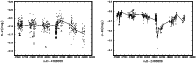
Figure B.1: Time plots of
and
indices of Tau based on various observations secured over the time interval covered by the Hipparcos  observations and shortly before and after it. Following notation
is used to distinguish data from various stations identified
in Table B.1:
01... empty circles, 08... empty triangles up, 09... empty squares,
15... small black dots, 73... empty diamonds. The solid lines are
connecting the normals points over 100 d in
and over 15 d in
- see the text for details.
observations and shortly before and after it. Following notation
is used to distinguish data from various stations identified
in Table B.1:
01... empty circles, 08... empty triangles up, 09... empty squares,
15... small black dots, 73... empty diamonds. The solid lines are
connecting the normals points over 100 d in
and over 15 d in
- see the text for details.
Open with DEXTER 
Figure B.2: Time plots of V photometry of
Tau based on various
observations secured over the time interval covered by the Hipparcos
observations and shortly before and after it. Following notation
is used to distinguish data from various stations identified
in Table B.1:
01... empty circles, 08... empty triangles up, 09... empty squares,
15... small black dots, 73... empty diamonds. The solid lines are
connecting the normals points over 100 d in
and over 15 d in .
Hipparcos
magnitudes transformed to Johnson V are shown by
black triangles down. See the text for the details.
- Station 49 - Limber Observatory: These observations were
secured and reduced by David McDavid at his private observatory as a part of
the international campaign on photometry of Be stars relative to 126 Tau.
We only added the standard Hvar
all-sky values of 126 Tau
of Table B.2 to the magnitude differences derived by DMD.
- Station 61 - Hipparcos: These observations were reduced to the
standard V and B magnitudes via the transformation formulæ derived by Harmanec (1998). Since the star underwent long-term colour variations
over the period 1989-93, covered by Hipparcos observations - as illustrated
by Fig. B.1 - we proceeded in the following way:
We first derived suitably chosen normal points of observational data
secured shortly before, during and shortly after the Hipparcos observations
at several stations. It turned out that the
changes were best
described by 100-d normals while the more pronounced
variations
were characterized by 15-d normals. Then we derived smooth lines passing
through the normal points with the help of a non-linear interpolation based on
Hermite polynomials using program INTEP by Hill (1982). With them,
we derived the appropriate values of
and
for the times
of individual
observations and these values were used to transform
individual Hipparcos observations to Johnson V after Harmanec (1998).
The resulting V magnitudes are compared with the true V observations
from other stations in Fig. B.2. A very satisfactory
agreement is seen there. Note also that Figs. B.1 and B.2
illustrate the level of (dis)agreement of magnitudes and indices from
individual observing stations.
- Station 73 - Piskéstetö: These
observations,
used in the paper by Percy et al. (1994), were obtained by Dr. M. Paparo and kindly put at our disposal for analyses in the form of magnitude differences Tau - 126 Tau and 121 Tau - 126 Tau, transformed to the standard system
and corrected for differential extinction. These observations will be
later published by their author and are not, therefore, included in
Table 4. Regrettably, the other set of photometry
used by Percy et al. (1994), obtained at Braeside Observatory, is not available.
- Station 95 - Tucson: These 8C all-sky observations were obtained
and published by Johnson et al. (1967) and we transformed them to the
magnitudes using the transformation formulæ derived by Harmanec & Bozic (2001).
Footnotes
- ... stars
- Based on new spectral and photometric observations from the following observatories: Dominion Astrophysical Observatory, Fairborn, Haute Provence, Hvar, Limber, McDonald, Ondrejov, and Ritter.
- ...
- Appendices are only available in electronic form at http://www.aanda.org
- ... level
- Thus, for instance,
where our measured peak value is, say,
 /
/
 (where
and
(where
and  are the peak and continuum fluxes, respectively), then in the alternative
notation the peak value is
are the peak and continuum fluxes, respectively), then in the alternative
notation the peak value is
 -
-
 .
.
- ...tex2html_cite_multiple_mark
- The program HEC13 with simple instructions is freely available at http://astro.troja.mff.cuni.cz/ftp/hec/HEC13
- ...Hill (1982)
- The program HEC36 with simple instructions on how to use it is freely available at http://astro.troja.mff.cuni.cz/ftp/hec/HEC36
- ... measurements
- These spectrograms, obtained and reduced to the form of wavelength calibrated and rectified spectra by their author, a French amateur astronomer C. Buil, are freely available to interested users as ASCII files at http://www.astrosurf.org/buil/us/becat.htm
- ... desirable
- There is one misprint on page 171 of Harmanec (1984): The correct RV at JD ..24563.639 is 34.7 km s-1, not 37.4 km s-1 as given there. Moreover, in several cases when more spectra have the same (inaccurate) JD, the H I and He I RVs do not correspond to the same spectrum.
- ... dates
- This program which handles data of various forms, together with brief instructions on how to use it, is freely available on the anonymous ftp server at http://astro.troja.mff.cuni.cz/ftp/hec/HEC19
All Tables
Table 1:
Slopes obtained by linear regression (y=a x+b) for V magnitude and H![]() EW data for all available data and several subsets.
EW data for all available data and several subsets.
Table 2:
Trial circular-orbit solutions for the RVs measured on the H![]() emission wings.
emission wings.
Table 3:
Trial solutions for the H I shell RVs,
He I RVs and a combination of H![]() emission-wing RVs with He I
RVs measured via cross-correlation in Jarad (1987).
emission-wing RVs with He I
RVs measured via cross-correlation in Jarad (1987).
Table 4:
Basic properties of the binary system estimated for
K=7 km s-1 and M1=11 ![]() and for several plausible orbital inclinations.
and for several plausible orbital inclinations.
Table A.1:
Journal of available RV observations of ![]() Tau.
Tau.
Table A.2:
Journal of available spectrophotometric H![]() observations of
observations of ![]() Tau .
Tau .
Table B.1:
Journal of available photometry of ![]() Tau with known times of observations.
Tau with known times of observations.
Table B.3:
Mean ![]() values for the check stars used at individual
observing stations derived differentially relative to their respective
comparison stars (cf. Table B.1). They illustrate how closely
the data could be transformed to a comparable standard system.
values for the check stars used at individual
observing stations derived differentially relative to their respective
comparison stars (cf. Table B.1). They illustrate how closely
the data could be transformed to a comparable standard system.
All Figures
|
|
Figure 1:
Sequence of H |
| In the text | |
![\begin{figure}\par\includegraphics[width=9cm]{10526fa1.eps}\par\includegraphics[...
...dth=9cm]{10526fa5.eps}\par\includegraphics[width=9cm]{10526fa6.eps}
\end{figure}](/articles/aa/full_html/2009/42/aa10526-08/img32.png)
|
Figure 2a:
Long-term RV, V/R, H |
| In the text | |
|
|
Figure 2b: The same as Fig. 2a for the time interval HJD 2442000-2445750. |
| In the text | |
|
|
Figure 2c: The same as Fig. 2a for the time interval HJD 2445750-2447750. |
| In the text | |
|
|
Figure 2d: The same as Fig. 2a for the time interval HJD 2447750-2449750. |
| In the text | |
|
|
Figure 2e: The same as Fig. 2a for the time interval HJD 2449750-2451750. |
| In the text | |
|
|
Figure 2f:
The same as Fig. 2a for the time
interval HJD 2451750-2454600. Additionally, the central intensity of the
H |
| In the text | |
|
|
Figure 3:
Long-term variation of the H I shell RVs, the V/R ratio of the Balmer emission lines of |
| Open with DEXTER | |
| In the text | |
|
|
Figure 4:
The ( |
| Open with DEXTER | |
| In the text | |
| |
Figure 5:
The time plot of all RVs of the H |
| Open with DEXTER | |
| In the text | |
|
|
Figure 6:
The orbital RV curve of the H |
| Open with DEXTER | |
| In the text | |
|
|
Figure 7:
Phase plot of several subsets of H I shell RVs, prewhitened for the long-term changes, vs. orbital phase. One can see
the gradual development of the bump near the minimum RV. In the bottom panel, the RVs of the H |
| Open with DEXTER | |
| In the text | |
|
|
Figure 8: Stelingwerf's PDM periodogram of the V/R ratio prewhitened for the long-term changes using spline functions. Solid line shows the analysis of simple double-peaked profiles, the dashed line the triple-peaked profiles. The arrow denotes the frequency of the orbital period. |
| Open with DEXTER | |
| In the text | |
|
|
Figure 9: Phase plots of individual V/R ( upper row) and V magnitude ( lower row) observations. Ephemeris from solution 2 are used and long-term changes were removed using Hermite polynomial interpolation scheme. Left: HJD < 2449000 subset. Right: HJD > 2449000 subset. |
| Open with DEXTER | |
| In the text | |
|
|
Figure 10: Orbital phase plots of individual V observations ( left panels) and the V/R ratio ( central and right panels) for individual observing seasons. Seasons with larger amplitude of orbital variations (HJD 2450726-2450918, 2451237-2451572 and 2453231-2453482 from left to right) are shown in the upper row, and the seasons with smaller amplitude of orbital variations (HJD 2451075-2451278, 2451850-2452002 and 2453611-2453844) are plotted in the lower row. |
| Open with DEXTER | |
| In the text | |
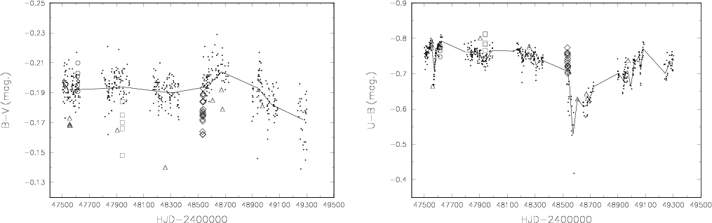
|
Figure B.1:
Time plots of |
| Open with DEXTER | |
| In the text | |

|
Figure B.2:
Time plots of V photometry of |
| Open with DEXTER | |
| In the text | |
Copyright ESO 2009
Current usage metrics show cumulative count of Article Views (full-text article views including HTML views, PDF and ePub downloads, according to the available data) and Abstracts Views on Vision4Press platform.
Data correspond to usage on the plateform after 2015. The current usage metrics is available 48-96 hours after online publication and is updated daily on week days.
Initial download of the metrics may take a while.