| Issue |
A&A
Volume 506, Number 2, November I 2009
|
|
|---|---|---|
| Page(s) | 811 - 828 | |
| Section | Stellar structure and evolution | |
| DOI | https://doi.org/10.1051/0004-6361/200810544 | |
| Published online | 27 August 2009 | |
A&A 506, 811-828 (2009)
Transport by gravito-inertial waves in differentially rotating stellar radiation zones
I - Theoretical formulation
S. Mathis1,2
1 - Laboratoire AIM, CEA/DSM-CNRS-Université Paris Diderot, IRFU/SAp Centre de Saclay, 91191 Gif-sur-Yvette, France
2 -
LUTH, Observatoire de Paris-CNRS-Université Paris Diderot, Place Jules Janssen, 92195 Meudon, France
Received 8 July 2008 / Accepted 3 July 2009
Abstract
Context. We examine the dynamics of low-frequency waves in
differentially rotating stellar radiation zones, the angular velocity
being taken as generally as possible depending both on radius and on
latitude in stellar interiors. The associated induced transport of
angular momentum, which plays a key role in the evolution of rotating
stars, is derived.
Aims. We focus on the wave-induced transport of angular
momentum, taking into account the Coriolis acceleration in the case of
strong radial and latitudinal differential rotation. We thus go beyond
the ``weak differential rotation'' approximation, where rotation is
almost a solid-body one plus a residual radial differential rotation.
As has been shown in previous works, the Coriolis acceleration modifies
such transport.
Methods. We built analytically a complete formalism that allows
the study of rotational transport in stellar radiation zones taking
into account the wave action modified by a general strong differential
rotation.
Results. The different approximations possible for low-frequency
waves in a differentially rotating stably stratified radiative region,
namely the traditional and the JWKB approximations, are examined and
discussed. The complete bidimensional structure of regular elliptic
gravito-inertial waves, which verify these approximations, is derived
and compared to those in the ``weak differential rotation'' case. Next,
associated transport of energy and of angular momentum in the vertical
and in the horizontal directions and the dynamical equations,
respectively for the mean radial differential rotation and the
latitudinal one, are obtained.
Conclusions. The complete formalism, which takes into account
low-frequency wave action, is derived and can be used for the study of
secular hydrodynamics of radiative regions and of the associated
mixing. The modification of waves due to general strong differential
rotation and their feed-back on the angular momentum transport are
treated rigourously. In a forthcoming paper (Paper II), this
formalism will be applied to the case of solar differential rotation.
However, the case of hyperbolic gravito-inertial waves should be
carefully studied.
Key words: hydrodynamics - waves - turbulence - methods: analytical - stars: rotation - stars: evolution
1 Introduction
The study of helioseismology, asteroseismology and powerful ground-based instrumentation dedicated to stellar physics is developing strongly (Turck-Chièze 2005, 2006, 2008; Aerts et al. 2008, and references therein) generating tight constraints on the internal structure and dynamics of stars. This is the reason why it is now necessary to build stellar models that take into account the dynamical processes from the birth of stars to their death.
A coherent picture of the dynamics of stellar radiation zones where the non-standard chemicals mixing takes place is thus required (cf. Zahn 2005).
A complex transport, which involves several mechanisms, takes place in these regions. First, rotation induces a large-scale circulation, the called meridional circulation, which acts to simultaneously transport angular momentum, chemicals and the magnetic field by advection. This circulation is due to differential rotation, to structural adjustments and to angular momentum losses at the surface (cf. Busse 1982; Zahn 1992; Talon et al. 1997; Maeder & Zahn 1998; Meynet & Maeder 2000; Garaud 2002b; Palacios et al. 2003-2006; Mathis & Zahn 2004, 2005; Rieutord 2006; Espinosa Lara & Rieutord 2007; Mathis et al. 2007; Decressin et al. 2009).
Next, differential rotation induces hydrodynamical turbulence through various instabilities such as the shear, the baroclinic and the multidiffusive ones. As in the terrestrial atmosphere, this turbulence acts to reduce its cause, namely the gradients of angular velocity (cf. Zahn 1983; Talon & Zahn 1997; Garaud 2001; Maeder 2003; Mathis et al. 2004).
On the other hand, rotation interacts with fossil magnetic fields. Then, the mean secular torque of the Lorentz force and the magnetohydrodynamical instabilities such as the Tayler-Spruit and the multidiffusive magnetic instabilities modify the transport of angular momentum and of chemicals (cf. Charbonneau & Mac Gregor 1993; Gough & McIntyre 1998; Garaud 2002a; Spruit 1999-2002; Menou et al. 2004; Maeder & Meynet 2004; Eggenberger et al. 2005; Braithwaite & Spruit 2005; Braithwaite 2006; Brun & Zahn 2006; Zahn et al. 2007).
Finally, internal gravity waves (hereafter IGWs), which are excited at the borders with convective zones, propagate through radiative regions where they extract or deposit angular momentum at the location where they are damped, leading to a modification of the angular velocity profile and consequently of the chemical distribution (cf. Goldreich & Nicholson 1989; Schatzman 1993; Kumar & Quataert 1997; Zahn et al. 1997; Ringot 1998; Talon et al. 2002; Talon & Charbonnel 2005; Rogers & Glatzmaier 2005b, 2006).
Here, we focus on IGWs. It is likely that there is a magnetic field in stellar radiation zones and more particularly at the level of the tachocline(s), at the border(s) between convection and radiation, which may be the zone of the storage of the mean axisymmetric part of the field toroidal component. In the presence of such a magnetic field, IGWs are then magneto-gravito-inertial waves (which are often called Magnetic Archimedean Coriolis (MAC) waves in geophysics) and the field acts as a filter to their vertical propagation (cf. Schatzman 1993; Barnes et al. 1998). In this work, we choose as a first step to ignore this interaction between IGWs and the magnetic field, which will be studied in a forthcoming paper, and to focus on purely hydrodynamical gravito-inertial waves.
In this context, it has now been undertaken to go beyond the
non-rotating approximation in the treatment of IGWs propagation and
induced transport. The Coriolis acceleration which strongly modifies
IGWs as soon as
![]() (where
(where ![]() and
and ![]() are respectively the wave's frequency and the inertial one) is then
taken into account. Depending on the excited wave spectrum which is
assumed (cf. Kumar et al. 1999; Rogers & Glatzmaier 2005b, 2006; Rogers et al. 2008,
and the detailed discussion in Sect. 4.2.1.), the Coriolis
acceleration effects have thus to be studied in a non-perturbative way
(cf. Fig. 2) mainly for
low-frequency gravito-inertial waves which may be excited in stellar
radiation zones in the neighborhood of the inertial frequency (
are respectively the wave's frequency and the inertial one) is then
taken into account. Depending on the excited wave spectrum which is
assumed (cf. Kumar et al. 1999; Rogers & Glatzmaier 2005b, 2006; Rogers et al. 2008,
and the detailed discussion in Sect. 4.2.1.), the Coriolis
acceleration effects have thus to be studied in a non-perturbative way
(cf. Fig. 2) mainly for
low-frequency gravito-inertial waves which may be excited in stellar
radiation zones in the neighborhood of the inertial frequency (![]() ).
).
To achieve this aim, the Coriolis acceleration has first been treated
using the traditional approximation, that can be applied in stellar
radiation zones in the super-inertial regime where
![]() in the case of uniform rotation (N is the Brunt-Väisälä frequency) (see for example Berthomieu et al. 1978; Friedlander 1987; Talon 1997; Mathis 2005). First numerical results using a stellar evolution code have been obtained (cf. Pantillon et al. 2007; Mathis et al. 2008).
in the case of uniform rotation (N is the Brunt-Väisälä frequency) (see for example Berthomieu et al. 1978; Friedlander 1987; Talon 1997; Mathis 2005). First numerical results using a stellar evolution code have been obtained (cf. Pantillon et al. 2007; Mathis et al. 2008).
However, in those previous works, a strong approximation on the differential rotation profile is assumed. In fact, the approximation of a weak differential rotation, where the rotation must be almost a solid-body one plus a residual radial differential rotation, is chosen in order to use the formalism coming from the treatment of Earth and planetary tides (Eckart 1960, Miles 1974). This is an imperative first step to understand the way in which the Coriolis acceleration modifies the transport due to IGWs.
Nevertheless, this approximation has to be relaxed in the case of a
real star where strong gradients of angular velocity can appear, both
in the radial and in the latitudinal directions, due to angular
momentum transport. First, as shown by Talon & Charbonnel (2005), strong radial ![]() -gradients
are created during the wave-induced angular momentum extraction.
Moreover, the angular velocity of the regions of waves excitation at
the borders of radiative regions with adjacent convection zones depends
both on radius and on latitude (for example the tachocline in the solar
case). This is the reason why we generalize the formalism, treating the
case of a general strong differential rotation, the angular velocity
-gradients
are created during the wave-induced angular momentum extraction.
Moreover, the angular velocity of the regions of waves excitation at
the borders of radiative regions with adjacent convection zones depends
both on radius and on latitude (for example the tachocline in the solar
case). This is the reason why we generalize the formalism, treating the
case of a general strong differential rotation, the angular velocity ![]() being a function both of the radius (r) and of the colatitude (
being a function both of the radius (r) and of the colatitude (![]() ), as can be potentially the case in stellar radiation zones during the evolution of stars.
), as can be potentially the case in stellar radiation zones during the evolution of stars.
First, we derive the equations ruling the dynamics of waves in a differentially rotating star. Then, we focus on the low-frequency waves in a differentially rotating stellar radiation zone. We present and discuss the different approximations that can be adopted there, namely the traditional and the JWKB ones, and we derive the associated dynamical equations. Then, we solve them to obtain the spatial structure of the wave pressure fluctuation and velocity field in the quasi-adiabatic approximation (cf. Press 1981; Zahn et al. 1997). A comparison with the weak differential rotation case is presented. Next, we study the induced transports of energy and of angular momentum by waves. We treat the matching of their pressure at the borders with adjacent convective regions where they are excited by turbulent movements. After a short review of the different models that can be adopted for such excitation which rules the waves spectrum, we derive the total transported flux of angular momentum. Finally, the associated dynamical equations governing the evolution of the mean differential rotation on an isobar and its latitudinal fluctuation are obtained, following the formalism used by Mathis & Zahn (2004) and Mathis & Zahn (2005). This allows us to treat for the first time the action of a general strong differential rotation on IGWs and their feed-back on the angular momentum transport, which is of major interest for stellar evolution.
In a forthcoming paper (Paper II), this formalism will be applied to the case of solar differential rotation.
2 Waves in a differentially rotating star
We have to solve the complete adiabatic inviscid system to treat the
wave dynamics in a differentially rotating star. It is formed by the
momentum equation
the continuity equation
the equation for the energy, which is given here in the adiabatic limit
and Poisson's equation for the gravitational potential

Dt is the Lagrangian derivative:
t is the time and r,
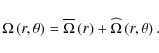
Equations (1-4) are linearized around the differentially rotating steady-state![]() . Each scalar field X (the density, the gravitational potential and the pressure) is expanded as the sum of its hydrostatic value,
. Each scalar field X (the density, the gravitational potential and the pressure) is expanded as the sum of its hydrostatic value,
![]() ,
and of the wave's associated fluctuation,
,
and of the wave's associated fluctuation,
![]() , as:
, as:
 |
(6) |
We obtain (cf. Unno et al. 1989):
where
Next, we have

and

The Lagrangian wave's displacement
Next,
![\begin{displaymath}{\widetilde X}
=\sum_{\sigma,m}\left\{X'\left(r,\theta\right)\exp\left[{\rm i}\left(m\varphi+\sigma t\right)\right]\right\},
\end{displaymath}](/articles/aa/full_html/2009/41/aa10544-08/img83.png)
![\begin{displaymath}\vec u
=\sum_{\sigma,m}\left\{\vec u'\left(r,\theta\right)\exp\left[{\rm i}\left(m\varphi+\sigma t\right)\right]\right\},
\end{displaymath}](/articles/aa/full_html/2009/41/aa10544-08/img84.png)
![\begin{displaymath}\vec \xi
=\sum_{\sigma,m}\left\{\vec \xi'\left(r,\theta\right)\exp\left[{\rm i}\left(m\varphi+\sigma t\right)\right]\right\},
\end{displaymath}](/articles/aa/full_html/2009/41/aa10544-08/img85.png) |
(14) |
Inserting Eqs. (12), (13) in Eq. (7), the following linearized momentum equation components are obtained:
where
 |
(18) |
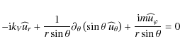
Next, the continuity equation (Eq. (8)), the energy equation in the adiabatic limit (Eq. (9)) and Poisson's equation (Eq. (10)) respectively become

![$\displaystyle \left.\frac{1}{r\sin\theta}\partial_{\theta}\left(\sin\theta u_{\theta}'\right)+\frac{{\rm i}m u_{\varphi}'}{r\sin\theta}\right]=0,$](/articles/aa/full_html/2009/41/aa10544-08/img94.png)
and
![\begin{displaymath}\frac{1}{r^2}\partial_{r}\left(r^2\partial_{r}\Phi'\right)\!+...
...right)\!-\!\frac{m^2}{\sin^2\theta}\Phi'\right]=4\pi G\rho'\!.
\end{displaymath}](/articles/aa/full_html/2009/41/aa10544-08/img98.png)
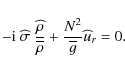
On the other hand, we get from Eq. (11):
 |
(22) |
where
In a differentially rotating region, the waves are Doppler-schifted
due to the differential rotation. Thus, the local wave angular velocity
that corresponds to the operator
![]() is:
is:
| (23) |
This Doppler-shift is an essential ingredient in the angular momentum deposition or extraction respectively through prograde (m<0) and retrograde waves (m>0) damping (see for example in Talon et al. 2002; note that we have chosen here the sign convention adopted by Lee & Saio 1997; and Mathis et al. 2008).
From now on, we neglect the non-spherical character of the hydrostatic
background due to the deformation associated with the centrifugal
acceleration,
![]() .
We thus stop the expansion of the equations to the first order in
.
We thus stop the expansion of the equations to the first order in
![]() where
where
![]() is the critical angular velocity of the star, R and M being respectively its radius and its mass. We thus have:
is the critical angular velocity of the star, R and M being respectively its radius and its mass. We thus have:
 |
(24) |
and the gravity
 |
(25) |
The general dynamical equations for waves in a differentially rotating star now being given, we focus our attention on radiative regions and on the approximations which can be applied there.
3 Low-frequency waves in a differentially rotating stellar radiation zone
3.1 The traditional approximation
In the general case, the operator which governs the spatial structure of the waves, the Poincaré operator, is of mixed type (elliptic and hyperbolic) and not separable (for a detailed discussion we refer the reader to Friedlander & Siegman 1982; Dintrans 1999; Dintrans et al. 1999; and to Dintrans & Rieutord 2000). This leads to the appearance of detached shear layers associated with the underlying singularities of the adiabatic problem that could be crucial for transport and mixing processes in stellar radiation zones, since they are the seat of strong dissipation (Stewartson & Richard 1969; Stewartson & Walton 1976; Dintrans et al. 1999; Dintrans & Rieutord 2000; Ogilvie & Lin 2004).
However, in the largest part of stellar radiation zones, we are in a regime where
![]() .
Since we are interested here in low-frequency waves where
.
Since we are interested here in low-frequency waves where
![]() ,
the traditional approximation, which consists of neglecting the latitudinal component of the rotation vector (
,
the traditional approximation, which consists of neglecting the latitudinal component of the rotation vector (
![]() with
with
![]() and
and
![]() ),
),
![]() ,
for all latitudes in the momentum equation, can be adopted in the case where
,
for all latitudes in the momentum equation, can be adopted in the case where
![]() when
when ![]() is uniform (see e.g. Eckart 1960; Lindzen & Chapman 1969; and Miles 1974; for a modern description in a stellar context see Nicholson 1989; Bildsten et al. 1996; Papaloizou & Savonije 1997; Lee & Saio 1997; Talon 1997). Then, it has been shown by Friedlander (1987)
that variable separation in radial and horizontal eigenfunctions
remains possible. This approximation has to be used carefully, as it
changes the nature of the Poincaré operator, and removes the
singularities and associated shear layers that appear. Therefore,
assuming solid-body rotation, it is only valid in the super-inertial
regime
is uniform (see e.g. Eckart 1960; Lindzen & Chapman 1969; and Miles 1974; for a modern description in a stellar context see Nicholson 1989; Bildsten et al. 1996; Papaloizou & Savonije 1997; Lee & Saio 1997; Talon 1997). Then, it has been shown by Friedlander (1987)
that variable separation in radial and horizontal eigenfunctions
remains possible. This approximation has to be used carefully, as it
changes the nature of the Poincaré operator, and removes the
singularities and associated shear layers that appear. Therefore,
assuming solid-body rotation, it is only valid in the super-inertial
regime
![]() ,
where the stratification dominates, that corresponds to the ergodic (regular) elliptic gravito-inertial mode family (the E1 modes in Dintrans et al. 1999; and Dintrans & Rieutord 2000). In the sub-inertial regime, where
,
where the stratification dominates, that corresponds to the ergodic (regular) elliptic gravito-inertial mode family (the E1 modes in Dintrans et al. 1999; and Dintrans & Rieutord 2000). In the sub-inertial regime, where
![]() ,
that corresponds to the equatorially trapped hyperbolic modes (the H2 modes in Dintrans et al. 1999; and Dintrans & Rieutord 2000),
the traditional approximation fails to reproduce the waves behaviour
and the complete momentum equation has to be solved (detailed examples
are given in Gerkema & Shrira 2005 and Gerkema et al. 2007).
,
that corresponds to the equatorially trapped hyperbolic modes (the H2 modes in Dintrans et al. 1999; and Dintrans & Rieutord 2000),
the traditional approximation fails to reproduce the waves behaviour
and the complete momentum equation has to be solved (detailed examples
are given in Gerkema & Shrira 2005 and Gerkema et al. 2007).
Therefore, we restrict ourselves here to the regular low-frequency waves for which the traditional approximation is usable. Its application domain in the case of general strong differential rotation will be discussed in Sect. 3.4.6.
Let us now adopt a local analysis of the problem in the simplest case of a uniform rotation (see also Lee & Saio 1997). The wave vector ![]() and Lagrangian displacement
and Lagrangian displacement ![]() are expanded as
are expanded as
 |
(26) |
 |
(27) |
where
For low-frequency waves in stably stratified regions, we can writte:
| (28) |
since
 |
(29) |
Next, using the results given in Unno et al. (1989), the following dispersion relation for the low-frequency gravito-inertial waves is obtained:
 |
(30) |
In this expression, the mixed behaviour of waves is clearly identified, the two terms corresponding respectively to the dispersion relations of IGWs,
 |
(31) |
The vertical wave vector is then larger than the horizontal one while the displacement vector is almost horizontal:
On the other hand, we get
![\begin{figure}
\par\includegraphics[width=8.8cm,clip]{10544f1.eps}
\end{figure}](/articles/aa/full_html/2009/41/aa10544-08/img139.png) |
Figure 1:
Wave types in differentially rotating stellar radiation zone and associated frequencies (where |
| Open with DEXTER | |
3.2 The JWKB approximation
Under the assumption that
![]() ,
each scalar field and each component of
,
each scalar field and each component of ![]() can be expanded using the JWKB approximation (see Landau & Lifchitz 1966; Fröman & Fröman 1965; Vallée & Soares 1998,
and references therein for mathematical details). In this case, the
vertical wave number is very large, the associated wave-length being
thus very small. Therefore, the spatial variation of the wave is very
rapid compared to that of the hydrostatic background (cf. compared to
those of
can be expanded using the JWKB approximation (see Landau & Lifchitz 1966; Fröman & Fröman 1965; Vallée & Soares 1998,
and references therein for mathematical details). In this case, the
vertical wave number is very large, the associated wave-length being
thus very small. Therefore, the spatial variation of the wave is very
rapid compared to that of the hydrostatic background (cf. compared to
those of
![]() ,
,
![]() and
and
![]() ).
Then, the wave spatial structure can be described by the product of a
plane-like wave function multiplied by a slowly varying envelope and we
obtain:
).
Then, the wave spatial structure can be described by the product of a
plane-like wave function multiplied by a slowly varying envelope and we
obtain:
with
and
 |
(38) |
The case of the fluctuation of the gravitational potential is particular since it is the sum of the fluctuating potential associated with the waves propagating in the studied radiation zone and of the one associated with the movements in the convection zone,
The JWKB phase function is given by:
![\begin{displaymath}{\mathcal S}\left(r\right)=\exp\left[{\rm i}\left(\int_{r}^{r...
... c}}k_{V}\left(r'\right){\rm d}r'+\frac{\pi}{2}\right)\right],
\end{displaymath}](/articles/aa/full_html/2009/41/aa10544-08/img153.png) |
(39) |
where the property of low-frequency waves given in Eq. (32) has been used to neglect
If the JWKB approximation is adopted, this also implies that the quasi-linear approximation, where the non-linear wave-wave interactions are neglected, is assumed.
Internal gravity waves - induced transport in stellar interiors was first studied by Press (1981). In this work, he emphasizes the possible non-linearity of the problem of IGWs excited by turbulent convective movements. He then shows that JWKB solutions, using crude prescriptions for the wave excitation, are at the limit between the linear and the non-linear regime. Furthermore, Rogers et al. (2008) obtain results where the non-linear regime develops in the case of an excited spectrum at the convection-radiation border computed through 2-D numerical simulations which account for a real solar stratification (see Sect. 4.2.1 for a more detailed description). This non-linear behaviour then shows that the quasi-linear approximation has to be used carefully depending on the excited spectrum that is assumed.
As discussed by Rogers et al. (2008), the quasi-linear approximation is relevant as long as the Froude number (Fr),
which gives the ratio between the wave-inertia term and the
stratification one, is small compared to unity. This number has been
computed by Rogers & Glatzmaier (2006;
cf. Fig. 4 in this paper) in the solar case using the same
numerical simulations as those discussed above. Then, they showed that
![]() in the bulk of the radiation zone, while it strongly grows in the
tachocline where IGWs are excited by the turbulent convection and at
the center because of the wave's geometrical focusing already
identified by Press (1981).
in the bulk of the radiation zone, while it strongly grows in the
tachocline where IGWs are excited by the turbulent convection and at
the center because of the wave's geometrical focusing already
identified by Press (1981).
Therefore, it is reasonable to adopt the quasi-linear approximation, being aware that it has to be used with caution in the excitation region and at the center.
3.3 Dynamical equations
Simultaneously using the traditional and the JWKB approximations and
assuming the anelastic one where sonic waves are filtered (i.e.
![]() ),
we derive the dynamical equations for low-frequency waves in
differentially rotating radiation zones. Substituting the expansion
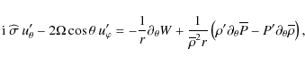
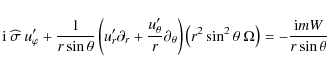
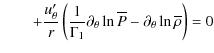
given in Eq. (33) to Eqs. (15-17), the final radial, latitudinal and azimuthal components of the momentum equation are obtained:
),
we derive the dynamical equations for low-frequency waves in
differentially rotating radiation zones. Substituting the expansion
given in Eq. (33) to Eqs. (15-17), the final radial, latitudinal and azimuthal components of the momentum equation are obtained:
where
 |
(43) |
The different simplifications adopted for each component of the momentum equation have to be detailed.
For its radial component (Eq. (15)), the traditional approximation, for which it is assumed that
![]() ,
allows one to neglect the radial component of the Coriolis acceleration
which is thus strongly dominated in the vertical direction by the
buoyancy restoring force. Furthermore, in a rigourous way, the inertial
term
,
allows one to neglect the radial component of the Coriolis acceleration
which is thus strongly dominated in the vertical direction by the
buoyancy restoring force. Furthermore, in a rigourous way, the inertial
term
![]() also has to be neglected since
also has to be neglected since
![]() .
However, it is first conserved here to make the historical link with
the works in the non-rotating case by Press (1981), Schatzman (1993) and Zahn et al. (1997) and with those in the uniformly rotating case by Pantillon et al. (2007) and Mathis et al. (2008) where it is conserved. Finally, the last right hand-side term
.
However, it is first conserved here to make the historical link with
the works in the non-rotating case by Press (1981), Schatzman (1993) and Zahn et al. (1997) and with those in the uniformly rotating case by Pantillon et al. (2007) and Mathis et al. (2008) where it is conserved. Finally, the last right hand-side term
![]() is not taken into account because of the anelastic approximation. Then, the latitudinal component (Eq. (16)) simplifies since
is not taken into account because of the anelastic approximation. Then, the latitudinal component (Eq. (16)) simplifies since
![]() , the other terms all being of the same order of magnitude and thus conserved. Finally, the term
, the other terms all being of the same order of magnitude and thus conserved. Finally, the term
![]() is neglected in the azimuthal component (Eq. (17)) since the wave's Lagrangian displacement is mostly horizontal (and thus
is neglected in the azimuthal component (Eq. (17)) since the wave's Lagrangian displacement is mostly horizontal (and thus
![]() )
for low-frequency IGWs
(cf. Eq. (32) and the discussion in Sect. 3.4.5).
)
for low-frequency IGWs
(cf. Eq. (32) and the discussion in Sect. 3.4.5).
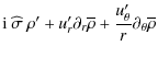
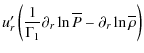
In addition, the continuity equation is![]() :
:
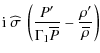
while the energy equation becomes
Finally, Poisson's equation is given by:

Cowling's approximation, in which the fluctuation of the gravitational potential is neglected in the momentum equation, is made (Cowling 1941). Therefore,
We are now ready to derive the wave spatial structure.
3.4 Spatial structure of the velocity field and associated properties
3.4.1 Spatial structure of the horizontal components of the velocity
The first step is to derive the spatial structure of the horizontal components of the velocity field as a function of
![]() .
To achieve this, we succesively eliminate
.
To achieve this, we succesively eliminate
![]() and
and
![]() between Eqs. (41) and (42). This leads to the following expressions for each of them:
between Eqs. (41) and (42). This leads to the following expressions for each of them:
![\begin{displaymath}{\widehat u}_{\theta}=\frac{\rm i}{r{\widehat \sigma}}\frac{1...
...os\theta}{\sin\theta}\left({\rm i}m{\widehat W}\right)\right],
\end{displaymath}](/articles/aa/full_html/2009/41/aa10544-08/img180.png)
![\begin{displaymath}{\widehat u}_{\varphi}=\frac{\rm i}{r{\widehat \sigma}}\frac{...
...widehat W}+\frac{{\rm i}m{\widehat W}}{\sin\theta}\right]\cdot
\end{displaymath}](/articles/aa/full_html/2009/41/aa10544-08/img181.png)
We have defined the local spin parameter
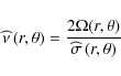 |
(49) |
and
 |
(50) |
Here, following Ogilvie & Lin (2004), we notice that in the case where
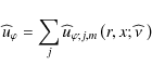
We make the hypothesis, which will be verified in the next section, that
![]() can be expanded as
can be expanded as
where wj,m is its jth spectral component and
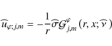
Then, it comes from Eq. (47) that:
 |
(52) |
where the jth spectral component is given by:
 |
(53) |
with
![\begin{displaymath}{\mathcal G}_{j,m}^{\theta}\left(r,x;\widehat{\nu}~\right)={\...
...;m}^{\theta}\left[w_{j,m}\left(r,x;\widehat\nu~\right)\right],
\end{displaymath}](/articles/aa/full_html/2009/41/aa10544-08/img193.png) |
(54) |
the linear operator
![\begin{displaymath}{\mathcal O}_{{\widehat \nu};m}^{\theta}=\frac{1}{\widehat{\s...
...eft(1-x^2\right)\frac{{\rm d}}{{\rm d}x}+m\widehat\nu x\right]
\end{displaymath}](/articles/aa/full_html/2009/41/aa10544-08/img195.png) |
(55) |
where
 |
(56) |
Similarly, we obtain from Eq. (48):
 |
(57) |
with
 |
(58) |
where
![\begin{displaymath}{\mathcal G}_{j,m}^{\varphi}\left(r,x;\widehat{\nu}~\right)={...
...m}^{\varphi}\left[w_{j,m}\left(r,x;\widehat\nu~\right)\right],
\end{displaymath}](/articles/aa/full_html/2009/41/aa10544-08/img199.png) |
(59) |
the linear operator
| |
= | ||
![$\displaystyle \times\left[-\left(\widehat\nu x-\left(1-x^2\right)\frac{\partial...
...ega}{\widehat\sigma}\right)\left(1-x^2\right)\frac{{\rm d}}{{\rm d}x}+m\right].$](/articles/aa/full_html/2009/41/aa10544-08/img203.png) |
(60) |
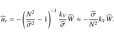
From the expressions obtained for
The spatial structure of the latitudinal and azimuthal components of the velocity field is now derived as a function of the pressure field. We have to derive its governing equation.
3.4.2 Spatial structure of the radial component of the velocity field and of the pressure
Eliminating the wave's density fluctuation
![]() between the radial momentum equation (Eq. (40)) and the energy equation (Eq. (45)), we obtain the relation between
between the radial momentum equation (Eq. (40)) and the energy equation (Eq. (45)), we obtain the relation between
![]() and
and
![]() :
:
 |
(61) |
Inserting it in the continuity equation (Eq. (44)), we get for wj,m, as defined in Eq. (51):
| |
= |  |
|
 |
(62) |
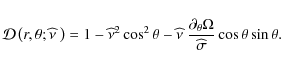
where the ``Generalized Laplace Operator'' (hereafter GLO),
| |
= |  |
|
![$\displaystyle -\frac{1}{\widehat\sigma}\left[\frac{m^2}{\widehat\sigma{\mathcal...
...}{\widehat\sigma{\mathcal D}\left(r,x;{\widehat\nu~}\right)}\right)\right]\cdot$](/articles/aa/full_html/2009/41/aa10544-08/img214.png) |
(63) |
The wj,m are thus the eigenfunctions of the GLO, namely
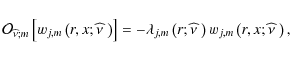
the eigenvalues
that determines the radial wave number kV;j,m at each r. The
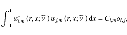
Following Ogilvie & Lin (2004), it can be shown that the GLO is self-adjoint, namely that
![\begin{displaymath}\int_{-1}^{1}f^{*}\left(x\right){\mathcal O}_{\widehat\nu;m}\...
...{\widehat\nu;m}\left[f\left(x\right)\right]{\rm d}x\right]^{*}
\end{displaymath}](/articles/aa/full_html/2009/41/aa10544-08/img221.png)
for any two functions f and g satisfying the regularity conditions at the poles (* is the complex conjugaison). The eigenvalues
 |
(66) |
where
It can be shown that the sign of
![]() depends on that of
depends on that of
![]() ;
see Ogilvie & Lin (2004) for a more detailed discussion. Singular points of Eq. (64) occur at the poles, or when
;
see Ogilvie & Lin (2004) for a more detailed discussion. Singular points of Eq. (64) occur at the poles, or when
![]() or
or
![]() vanish (these are respectively the corotation resonance or the Lindblad one, as has been discussed).
vanish (these are respectively the corotation resonance or the Lindblad one, as has been discussed).
The boundary conditions have been given by Ogilvie & Lin (2004): close to the north pole, the two independent solutions are
![]() and
and
![]() in the case where
in the case where ![]() while we get
while we get
![]() or
or
![]() when m=0. The condition that the wj,m
are bounded selects the regular solution. A similar condition is
required at the south pole. This provides the two boundary conditions
for our eigenvalue problem.
when m=0. The condition that the wj,m
are bounded selects the regular solution. A similar condition is
required at the south pole. This provides the two boundary conditions
for our eigenvalue problem.
Moreover, as it can be seen immediately, eigenvalues depend on the radial coordinate, r. Ogilvie & Lin (2004) describe a ``parametric'' dependance, since
![]() is a differential operator in x
only. We prefer here to say that the use of the JWKB solution allows us
to reduce the problem of a bidimensionnal partial differential equation
in r and
is a differential operator in x
only. We prefer here to say that the use of the JWKB solution allows us
to reduce the problem of a bidimensionnal partial differential equation
in r and ![]() to the one of a differential equation in x for each r, the obtained solution being also completely 2D without any variable separation in r and x. This is because the GLO depends on x, but also on r through
to the one of a differential equation in x for each r, the obtained solution being also completely 2D without any variable separation in r and x. This is because the GLO depends on x, but also on r through
![]() and
and
![]() .
In this way, even in the case of a shellular rotation
.
In this way, even in the case of a shellular rotation
![]() ,
the problem is not separable, the only separable case being the weak differential rotation one (see Sect. 3.4.5).
,
the problem is not separable, the only separable case being the weak differential rotation one (see Sect. 3.4.5).
3.4.3 Phase and group velocities; radiative damping
Using the wave's dispersion relation given in Eq. (65), the monochromatic vertical group velocity is derived
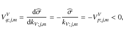 |
(67) |
Vp;j,mV being the associated vertical phase velocity; it is negative here since we are studying the case of a solar-type star where waves are excited by the turbulent convection in an upper external envelope (the opposite is obtained in the case of massive stars where waves are excited by a convective core).
Moreover, the vertical radiative damping (we have to remember that
![]() )
is given by (see for example Kumar et al. 1999):
)
is given by (see for example Kumar et al. 1999):
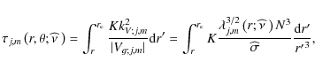
K being the thermal diffusivity. One can note that the non-uniform rotation modifies the damping rate since
As in Press (1981) and Zahn et al. (1997),
we adopt here the quasi-adiabatic approximation. In this way, the
pressure fluctuation and the velocity field of a monochromatic wave are
given by:
| |
= | (69) | |
| = | (70) |
3.4.4 Final pressure field and velocity field
Using the results reported previously, the pressure field
![]() and the velocity field
and the velocity field ![]() of
the low-frequency waves in a differentially rotating radiation zone can
be derived. Assuming the quasi-adiabatic approximation, we obtain for
the pressure field:
of
the low-frequency waves in a differentially rotating radiation zone can
be derived. Assuming the quasi-adiabatic approximation, we obtain for
the pressure field:
 |
(71) |
where
the phase function
 |
(73) |
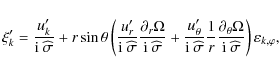
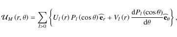
Then, we get for the velocity field:
![\begin{displaymath}\vec u=\sum_{k=\left\{r,\theta,\varphi\right\}}\left[\sum_{\s...
...,m}\left(r,\theta,\varphi,t\right)\right]\widehat{\vec{e}}_{k}
\end{displaymath}](/articles/aa/full_html/2009/41/aa10544-08/img249.png) |
(74) |
where
![$\displaystyle \frac{\widehat\sigma}{N}\frac{\lambda^{1/2}_{j,m}\left(r;\widehat...
...(r,\theta;\widehat\nu\right)\sin\left[\Phi_{j,m}\left(r,\varphi,t\right)\right]$](/articles/aa/full_html/2009/41/aa10544-08/img251.png)
![$\displaystyle -\frac{\widehat\sigma}{r}{\mathcal G}_{j,m}^{\theta}\left(r,\theta;\widehat\nu~\right)\cos\left[\Phi_{j,m}\left(r,\varphi,t\right)\right]$](/articles/aa/full_html/2009/41/aa10544-08/img253.png)
![$\displaystyle \frac{\widehat\sigma}{r}{\mathcal G}_{j,m}^{\varphi}\left(r,\theta;\widehat\nu~\right)\sin\left[\Phi_{j,m}\left(r,\varphi,t\right)\right]$](/articles/aa/full_html/2009/41/aa10544-08/img255.png)
On the other hand, since we have to use it to compute the vertical flux of angular momentum (see Sect. 4.1.2, Bretherton 1969; and Pantillon et al. 2007), we derive from Eq. (11):
 |
(78) |
with
3.4.5 Discussion of the weak differential rotation case
In the weak differential rotation case where the angular velocity is expanded such that
 |
(80) |
with
 |
(81) |
where
The GLO,
![]() ,
then reduces to the classical Laplace's tidal operator
,
then reduces to the classical Laplace's tidal operator
![]() :
:
![$\displaystyle {\mathcal O}_{{\widehat \nu}_{\rm s};m}=\frac{1}{\sigma_{\rm s}^{...
...^2}+m\nu_{\rm s}\frac{1+\nu_{\rm s}^{2}x^2}{1-\nu_{\rm s}^{2}x^2}\right)\right]$](/articles/aa/full_html/2009/41/aa10544-08/img267.png) |
(82) |
of which the eigenfunctions are the usual Hough's functions
The dispersion relation obtained in Eq. (65) is then given by
where the classical eigenvalues for the Laplace tidal operator,
Finally, the operators
![]() and
and
![]() are simplified
are simplified
| |
= | ||
| = | ![$\displaystyle \frac{1}{\sigma_{\rm s}^{2}}\times\left[\frac{1}{\left(1\!-\!\nu_...
...ft(1\!-\!x^2\right)\frac{{\rm d}}{{\rm d}x}\!+\!m\nu_{\rm s} x\right]\right]\!,$](/articles/aa/full_html/2009/41/aa10544-08/img277.png) |
(84) | |
| = | |||
| = | ![$\displaystyle \frac{1}{\sigma_{\rm s}^{2}}\times\left[\frac{1}{\left(1\!-\!\nu_...
..._{\rm s} x\left(1\!-\!x^2\right)\frac{{\rm d}}{{\rm d}x}\!+\!m\right]\right]\!,$](/articles/aa/full_html/2009/41/aa10544-08/img280.png) |
(85) |
where the linear differential operators
We thus obtain a separation of variables in r and ![]() ,
as in Lee & Saio (1997), Mathis (2005), Pantillon et al. (2007) and Mathis et al. (2008), with in the adiabatic case:
,
as in Lee & Saio (1997), Mathis (2005), Pantillon et al. (2007) and Mathis et al. (2008), with in the adiabatic case:
 |
(86) |
and
| |
= |  |
(87) |
| = |  |
(88) |
where we recall the respective definition of
| |
= | (89) | |
| = | (90) |
Finaly, the thermal damping rate becomes using Eq. (83):
3.4.6 The traditional approximation in the case of general differential rotation
In the weak differential rotation case (see Sect. 3.4.5), the
traditional approximation can be applied in spherical shell(s) where
| (92) |
thus as long as
where
![\begin{figure}
\par\includegraphics[width=8.5cm,clip]{10544f2.eps}
\end{figure}](/articles/aa/full_html/2009/41/aa10544-08/img305.png) |
Figure 2:
|
| Open with DEXTER | |
![\begin{figure}
\par\includegraphics[width=8.5cm,clip]{10544f3.eps}
\end{figure}](/articles/aa/full_html/2009/41/aa10544-08/img310.png) |
Figure 3:
|
| Open with DEXTER | |
In the case of a general strong differential rotation (
![]() ), the traditional approximation can be applied as long as
), the traditional approximation can be applied as long as
![]() and
and
![]() in spherical shell(s) where
in spherical shell(s) where
that corresponds to the regular elliptic gravito-inertial waves.
In the other spherical shell(s), where both
![]() and
and
![]() ,
critical surfaces appear, on which
,
critical surfaces appear, on which
![]() .
Then, the traditional approximation fails to reproduce the wave
behaviour since the adiabatic wave operator (and velocity field)
becomes singular and thus it should be abandoned (Friedlander 1987), as in the sub-inertial regime in the weak differential rotation case.
.
Then, the traditional approximation fails to reproduce the wave
behaviour since the adiabatic wave operator (and velocity field)
becomes singular and thus it should be abandoned (Friedlander 1987), as in the sub-inertial regime in the weak differential rotation case.
To illustrate this, we consider the radiation zone of a solar-type
star. Its external border with the convective envelope, where a
tachocline layer is assumed, is located at the radius
![]() (in the Sun,
(in the Sun,
![]() ;
see for example Schatzman et al. 2000).
;
see for example Schatzman et al. 2000).
We consider three different angular velocity profiles.
First, we define a radial differential rotation,
![]() ,
which has a smooth gradient troughout the radiative core:
,
which has a smooth gradient troughout the radiative core:
![\begin{displaymath}\Omega_{1}\left(r\right)=\overline\Omega_{\rm s}\left[1+{\rm sinc}\left(\pi\frac{r}{R_{\rm T}}\right)\right],
\end{displaymath}](/articles/aa/full_html/2009/41/aa10544-08/img316.png) |
(95) |
where
Next, we consider a second radial differential rotation
![\begin{displaymath}\Omega_{2}\left(r\right)=\overline\Omega_{\rm s}\left[2-A_{\rm c}{\rm Erf}\left(\frac{r-r_{\rm c}}{l_{\rm c}}\right)\right],
\end{displaymath}](/articles/aa/full_html/2009/41/aa10544-08/img319.png) |
(96) |
which has a strong gradient located in the core of the radiation zone (
![\begin{figure}
\par\includegraphics[width=8.5cm,clip]{10544f4.eps}
\end{figure}](/articles/aa/full_html/2009/41/aa10544-08/img326.png) |
Figure 4:
Rotation frequencies
|
| Open with DEXTER | |
Finally, we study a third differential rotation that depends only on the colatitude (![]() ),
),
![]() ,
to illustrate the effect of the latitudinal gradient of the rotation
frequency. We choose here the horizontal differential rotation obtained
through helioseismic inversions at the bottom of the solar convective
envelope (Thompson et al. 2003):
,
to illustrate the effect of the latitudinal gradient of the rotation
frequency. We choose here the horizontal differential rotation obtained
through helioseismic inversions at the bottom of the solar convective
envelope (Thompson et al. 2003):
 |
(97) |
where
![\begin{figure}
\par\includegraphics[width=8.5cm,clip]{10544f5.eps}
\end{figure}](/articles/aa/full_html/2009/41/aa10544-08/img332.png) |
Figure 5:
Rotation frequency
|
| Open with DEXTER | |
First,
![]() is considered. In the case of radial differential rotation,
is considered. In the case of radial differential rotation,
![]() ,
its variation is directly given by the rotation frequency profiles modulated by
,
its variation is directly given by the rotation frequency profiles modulated by
![]() (cf. Fig. 6 where we focus on axisymmetric waves (i.e. m=0)
that filters out the Doppler shift and thus allows us to isolate the
effects of the differential rotation itself). Then, the surface
(cf. Fig. 6 where we focus on axisymmetric waves (i.e. m=0)
that filters out the Doppler shift and thus allows us to isolate the
effects of the differential rotation itself). Then, the surface
![]() ,
which corresponds to
,
which corresponds to
![]() in the weak differential rotation case, is given by
in the weak differential rotation case, is given by
![]() .
.
![\begin{figure}
\par\includegraphics[width=8.5cm,clip]{10544f6a.eps}\par\includegraphics[width=8.5cm,clip]{10544f6b.eps}
\end{figure}](/articles/aa/full_html/2009/41/aa10544-08/img343.png) |
Figure 6:
Top:
|
| Open with DEXTER | |
In the case of the latitudinal rotation,
![]() ,
we obtain the same behaviour, the surface
,
we obtain the same behaviour, the surface
![]() being given by
being given by
![]() (cf. Fig. 7 for m=0).
(cf. Fig. 7 for m=0).
![\begin{figure}
\par\includegraphics[width=8.5cm,clip]{10544f7.eps}
\end{figure}](/articles/aa/full_html/2009/41/aa10544-08/img349.png) |
Figure 7:
|
| Open with DEXTER | |
In the case of a strong differential rotation, the traditional
approximation can be applied in spherical shell(s) where
(cf. Eq. (94))
 |
|||
| (98) |
For a radial differential rotation, this corresponds to spherical shell(s) where
![\begin{displaymath}4\left[\Omega\left(r\right)\right]^2\cos^2\theta<{\widehat \s...
...{ }\hbox{and}\hbox{ }\forall\theta\in\left[0,\pi\right]\right)
\end{displaymath}](/articles/aa/full_html/2009/41/aa10544-08/img353.png)
that leads to
The cases of
![]() and
and
![]() are illustrated in Fig. 8 for m=0. In each of them, a forbidden spherical shell appears, where both
are illustrated in Fig. 8 for m=0. In each of them, a forbidden spherical shell appears, where both
![]() and
and
![]() (the adiabatic waves velocity field is singular where
(the adiabatic waves velocity field is singular where
![]() ), that corresponds to an higher rotation frequency. Its spatial location and radius depend on the
), that corresponds to an higher rotation frequency. Its spatial location and radius depend on the
![]() profile and it becomes smaller as the frequency increases.
profile and it becomes smaller as the frequency increases.
![\begin{figure}
\par\includegraphics[width=18cm,clip]{10544f8a.eps}\par\includegraphics[width=18cm,clip]{10544f8b.eps}
\end{figure}](/articles/aa/full_html/2009/41/aa10544-08/img364.png) |
Figure 8:
Top:
|
| Open with DEXTER | |
Finally, in the case of a latitudinal differential rotation, such as
![]() ,
the allowed domain, in which the traditional approximation can be
applied, is modified both by the rotation frequency profile and its
latitudinal gradient. This is shown in Fig. 9 for m=0, which has to be compared with the weak differential rotation case studied in Fig. 3.
,
the allowed domain, in which the traditional approximation can be
applied, is modified both by the rotation frequency profile and its
latitudinal gradient. This is shown in Fig. 9 for m=0, which has to be compared with the weak differential rotation case studied in Fig. 3.
4 Wave-induced transport of angular momentum
From now on, we study the wave-induced transport of energy and of angular momentum in spherical shell(s) where the traditional approximation can be applied. In other words, we focus on the transport associated with the regular elliptic gravito-inertial waves, the hyperbolic regime being beyond the scope of this paper.
Therefore, since we are now working in allowed spherical shell(s), all the classical averages over longitudes (![]() )
and co-latitudes (
)
and co-latitudes (![]() )
can be defined.
)
can be defined.
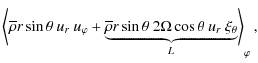
4.1 Fluxes transported by a monochromatic wave
The goal of this paper is to study the influence of a general differential rotation on low-frequency waves and their feed-back on the transport of angular momentum. The first step in this part of the work is now to derive the fluxes of energy and of angular momentum carried by a monochromatic wave.
4.1.1 Fluxes of energy
In the general bidimensional case which is studied here, the flux of
energy in the direction of the kth coordinate is given by the acoustic flux (see Lighthill 1978; Press 1981; Unno et al. 1989)![]()
 |
(99) |
where P'j,m and the uk;j,m components (where
Radial flux of energy
The flux of energy transported in the radial direction is thus given by
 |
(100) |
Using the expression derived in Eqs. (72) and (75), we thus obtain:
![\begin{displaymath}{\mathcal F}_{V;j,m}^{\rm E}=-\frac{1}{2}\overline\rho\frac{\...
...lambda_{j,m}^{1/2}}{r}w_{j,m}^{2}\exp\left[-\tau_{j,m}\right].
\end{displaymath}](/articles/aa/full_html/2009/41/aa10544-08/img374.png)
![\begin{figure}
\par\includegraphics[width=9cm,clip]{10544f9.eps}
\end{figure}](/articles/aa/full_html/2009/41/aa10544-08/img379.png) |
Figure 9:
|
| Open with DEXTER | |
Horizontal flux of energy
In the same way, the flux of energy transported in the
horizontal direction is given by the sum of fluxes in the latitudinal
and azimuthal directions:
 |
(102) |
where

Using Eqs. (72, 77), we get:
 |
(103) |
due to the quadrature between P'j,m and
![\begin{displaymath}{\mathcal F}_{H;j,m}^{\rm E}={\mathcal F}_{\varphi;j,m}^{\rm ...
...{j,m}{\mathcal G}_{j,m}^{\varphi}\exp\left[-\tau_{j,m}\right].
\end{displaymath}](/articles/aa/full_html/2009/41/aa10544-08/img384.png) |
(104) |
4.1.2 Fluxes of angular momentum
The equation for the transport of angular momentum is given by (see for example Brun & Toomre 2002; or Mathis & Zahn 2004):
Since this work is dedicated to the secular rotational transport during the evolution of the star, the Lagrangian time derivative
| |
= |  |
(106) |
| = | (107) |
Radial component of the flux of angular momentum
The radial component of the monochromatic flux of angular momentum is then given by:
that becomes, once again using Eqs. (75, 77, 79):
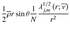
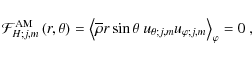
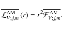
Following Zahn et al. (1997), the mean vertical flux of angular momentum on an isobar is defined:
 |
(110) |
where
![$\displaystyle \overline{{\mathcal F}_{V;j,m}^{\rm AM}}=\frac{3}{8}\overline\rho...
...{\mathcal G}_{j,m}^{\theta}\right)\exp\left[-\tau_{j,m}\right]\right>_{\theta}.$](/articles/aa/full_html/2009/41/aa10544-08/img408.png)
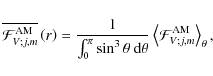
Horizontal component of the flux of angular momentum
In the same way, we derive the latitudinal component of the monochromatic flux of angular momentum:
due to the quadrature between
4.1.3 Action (luminosity) of angular momentum
We can define the monochromatic action of angular momentum (that is called luminosity of angular momentum in stellar physics)
 |
(113) |
In the adiabatic case, where the radiative damping is not taken into account, this action of angular momentum (as well as the action of energy, namely
 |
(114) |
where
![\begin{displaymath}{\mathcal L}_{V;j,m}^{\rm AM}\left(r,\theta\right)={\mathcal ...
...m AM}\left(r_{\rm c},\theta\right)\exp\left[-\tau_{j,m}\right]
\end{displaymath}](/articles/aa/full_html/2009/41/aa10544-08/img415.png)
that gives
where
| (117) | |||
We have defined the local spin parameter at
 |
(118) |
where
| (119) |
As in Eqs. (111, 112), the mean action of angular momentum on an isobar is derived:
 |
(120) |
We thus obtain:
![$\displaystyle \overline{{\mathcal L}_{V;j,m}^{\rm AM}}=\frac{3}{8}\overline\rho...
...theta}\right)\right]_{r=r_{\rm c}}\exp\left[-\tau_{j,m}\right]\right>_{\theta}.$](/articles/aa/full_html/2009/41/aa10544-08/img425.png)
To derive the total angular momentum flux transported by IGWs, the match between the turbulent convection and the waves now has to be examined very carefully to obtain a correct treatment of their excitation.
4.2 Waves excitation by convection and total action of angular momentum
4.2.1 Energy flux transfer
The first method to treat the wave excitation problem is to relate the
flux of angular momentum to the wave-energy flux. Following the
procedure used for the non-rotating and the weak differential rotation
cases (cf. Zahn et al. 1997; Pantillon et al. 2007), we define
![]() such that:
such that:
 |
(122) |
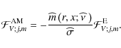
Using the respective expressions of
![\begin{displaymath}{\widehat m}\left(r,x;\widehat \nu~\right)=\frac{\sin\theta~{...
...os\theta~{\mathcal G}_{j,m}^{\theta}\right]}{w_{j,m}^{2}}\cdot
\end{displaymath}](/articles/aa/full_html/2009/41/aa10544-08/img430.png) |
(123) |
This can be understood as the efficiency transmission factor that gives us, for each frequency and each latitude, the energy transfer from the convective movements to the waves. It also allows us to quantify the bias in the excitation between prograde and retrograde waves.
In the non-rotating case (![]() ), we get
), we get
![]() and therefore
and therefore
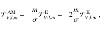 |
(124) |
where
Using Eq. (115), we thus have:
![\begin{displaymath}{\mathcal L}_{V;j,m}^{\rm AM}\left(r,x;\widehat\nu~\right)={\...
...rm c},x;\widehat\nu_{\rm c}\right)\exp\left[-\tau_{j,m}\right]
\end{displaymath}](/articles/aa/full_html/2009/41/aa10544-08/img436.png) |
(125) |
where
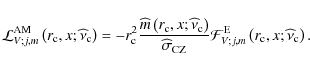 |
(126) |
Taking all the spectrum of excited waves,
![$\displaystyle {\mathcal L}_{V}^{\rm AM}\left(r,x;\widehat\nu~\right)=
-r_{\rm c...
...x;{\widehat\nu}_{\rm c}\right)\exp\left[-\tau_{j,m}\right]\right\}{\rm d}\sigma$](/articles/aa/full_html/2009/41/aa10544-08/img439.png)
and
![$\displaystyle \overline{{\mathcal L}_{V}^{\rm AM}}\left(r\right)=
-r_{\rm c}^{2...
...\rm c}\right)\exp\left[-\tau_{j,m}\right]\right>_{\theta}\right\}{\rm d}\sigma.$](/articles/aa/full_html/2009/41/aa10544-08/img440.png) |
(128) |
The transported flux of angular momentum now being derived, it is necessary to look for a robust prescription for the excited wave energy spectrum at
4.2.2 Amplitude of each monochromatic wave
The second method to approach the problem of wave excitation is to work on the amplitude of each monochromatic wave.
We assume that the pressure field in the convection zone at
![]() can be expanded formally in the following Fourier form:
can be expanded formally in the following Fourier form:
| |
= | ||
| (129) |
where the
 |
(130) |
where the aj,m projection coefficients are given by:
![\begin{displaymath}a_{j,m}\left(r_{\rm c};\sigma\right)=\frac{\left<W_{{\rm CZ};...
...a;{\widehat \nu}_{\rm c}\right)\right]^2\right>_{\theta}}\cdot
\end{displaymath}](/articles/aa/full_html/2009/41/aa10544-08/img449.png) |
(131) |
Assuming the continuity of the pressure between the turbulent movements in the convection zone and the waves inside the radiative region, summing over the spectrum of excited frequencies, the total action of angular momentum associated with waves is derived
with its associated average on an isobar
where
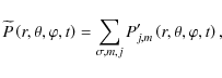
In every case, the pressure field at
![]() can be expanded in spherical harmonics:
can be expanded in spherical harmonics:
| (134) |
where the normalized associated Legendre polynomials have been defined:
![\begin{displaymath}{\widetilde P}_{l}^{m}\left(\cos\theta\right)=\left(-1\right)...
...right)!}\right]^{\frac{1}{2}}P_{l}^{m}\left(\cos\theta\right).
\end{displaymath}](/articles/aa/full_html/2009/41/aa10544-08/img456.png) |
(135) |
The
| |
= |  |
|
| (136) |
where
 |
(137) |
the projection of each spherical function on the wj,m being given by:
![\begin{displaymath}{\mathcal P}_{l,m}^{j}\left(r_{\rm c};{\widehat\nu}_{\rm c}\r...
...a;{\widehat \nu}_{\rm c}\right)\right]^2\right>_{\theta}}\cdot
\end{displaymath}](/articles/aa/full_html/2009/41/aa10544-08/img461.png) |
(138) |
Then,
| |
= | ||
![$\displaystyle \times{\left.\sin\theta\left[{\widehat \sigma}^{2}~w_{j,m}\left({...
...\right)\right]_{r=r_{\rm c}}\exp\left[-\tau_{j,m}\right]\right\}}{\rm d}\sigma,$](/articles/aa/full_html/2009/41/aa10544-08/img464.png) |
(139) |
with its associated average on an isobar
| |
= | ![$\displaystyle \frac{3}{8}\overline\rho_{\rm c}r_{\rm c}\frac{1}{N_{\rm c}}\int_...
...\mathcal P}_{l,m}^{j}\left(r_{\rm c};\widehat\nu_{\rm c}\right)\right]^2\right.$](/articles/aa/full_html/2009/41/aa10544-08/img466.png) |
|
![$\displaystyle \times{\left.\left<\sin\theta\left[{\widehat \sigma}^{2}~w_{j,m}\...
...r=r_{\rm c}}\exp\left[-\tau_{j,m}\right]\right>_{\theta}\right\}}{\rm d}\sigma.$](/articles/aa/full_html/2009/41/aa10544-08/img467.png) |
(140) |
4.2.3 Discussion
This search for a prescription for excitation remains major unsolved and debated question in wave-induced transport theory. To study this, different approaches have been adopted.
The first analytical one consists of deriving, using phenomenological prescritions, the energy flux transmission between the turbulent convective movements and the IGWs using the match of the wave pressure fluctuation with that of the turbulent convection. A Kolmogorov turbulent energy spectrum is assumed. This procedure is described in detail in Press (1981), Garciá López & Spruit (1991) and Zahn et al. (1997) in the non-rotating case and by Pantillon et al. (2007) in the case where the Coriolis acceleration is taken into account.
The second semi-analytical approach consists of deriving, in the most consistent possible way, the wave amplitude by describing their stochastic volumetric excitation by the convective Reynolds stresses and the turbulent entropy advection. This method takes into account both the spatial and the temporal correlations between turbulent eddies and waves. The formalisms follow the first work by Goldreich et al. (1994) which was devoted to solar p-modes and adapted to IGWs by Kumar et al. (1999). These first contributions assumed a Kolmogorov energy spectrum. These works were then generalized by Samadi et al. (2001a,b) in order to take into account a general turbulent energy spectrum which can be extracted from realistic 3-D numerical simulations of turbulent convection in stellar interiors and by Belkacem et al. (2008a,b) who derived a rigourous treatment of the excitation accounting for the non-radial character of the modes that is crucial in the case of IGWs for which the displacement is mostly horizontal. Finally, the Coriolis acceleration is now taken into account (Mathis et al. 2008; Belkacem 2008) and the generalized formalism has now to be applied to gravito-inertial waves.
Penetrative convection is also an efficient process to generate IGWs. This was first investigated by Townsend (1965, 1966) in the case of atmospheric flows. Then, in the stellar context, Montalbán (1994), Montalbán & Schatzman (1996-2000), following Townsend (1966), used several models for wave excitation by plumes in order to study the problem of light element mixing induced by IGWs (see also the work by Lo & Schatzman 1997; and Lo 1997, for the case of convective cores). However, they considered that waves are generated solely by turbulence inside plumes and they did not investigate the generation of waves caused by the impact of plumes on the stably stratified region that has been undertaken (cf. Belkacem 2008).
The major approach to obtain prescriptions for the wave energy spectrum in this case consists of computing numerical simulations of turbulent penetrative convection at the interface between convective and radiative regions. Such simulations have shown IGW excitation (see for example Hurlburt et al. 1986, 1994; Andersen 1994; Brummell et al. 2002; Browning et al. 2004; Rogers & Glatzmaier 2005; Rogers et al. 2006) but specific work has to be undertaken to provide a quantitative estimate of the amplitude and of the spectrum of waves.
Initial work dedicated to such a study has been completed in 2-D Cartesian geometry by Kiraga et al. (2003).
In this work, the assumed stratification is polytropic and the authors
add a viscous boundary layer at the bottom of the stable zone in order
to avoid the reflexion of excited waves and thus the appearance of
normal modes in the simulation box. Their main results are that
phenomenological semi-analytical models (the Garcià-Lopez & Spruit
one, hereafter GLS91; or the plume model by Rieutord & Zahn 1995,
hereafter RZ95) significantly underestimate the flux of IGWs by a
factor of 100 (GLS91) and 10 (RZ95) compared to 2-D direct numerical
simulations. On the other hand, in the domain
![]() ,
the numerically obtained wave spectrum is much broader than those
predicted using GLS91 which results in a lack of high frequency waves
and RZ95 where low frequencies are missing. However, the authors
emphasized that 2-D simulations probably produce stronger downflows
compared to more realistic 3-D simulations. This is the reason why
Kiraga et al. (2005)
revisited their own work comparing their previous results with those
obtained in a 3-D Cartesian box using the same stratification where
downdrafts are significantly less vigorous. On one hand, the excited
IGWs have lower amplitude. On the other hand, the wave energy flux
increases with the depth of the convective layer.
,
the numerically obtained wave spectrum is much broader than those
predicted using GLS91 which results in a lack of high frequency waves
and RZ95 where low frequencies are missing. However, the authors
emphasized that 2-D simulations probably produce stronger downflows
compared to more realistic 3-D simulations. This is the reason why
Kiraga et al. (2005)
revisited their own work comparing their previous results with those
obtained in a 3-D Cartesian box using the same stratification where
downdrafts are significantly less vigorous. On one hand, the excited
IGWs have lower amplitude. On the other hand, the wave energy flux
increases with the depth of the convective layer.
In the same way, Dintrans et al. (2005)
proposed a quantitative investigation of the spectrum, the amplitude
and the life-time of IGWs excited by penetrative convection in
solar-like stars using 2-D numerical simulations of compressible
convection assuming that the gas is monoatomic and perfect. The wave
generation is studied from the linear response of the radiative zone to
the plume penetration using projections onto the g-mode linear eigenfunctions. The authors show that up to ![]() of the total kinetic energy is transmitted to IGWs during times of significant excitation.
of the total kinetic energy is transmitted to IGWs during times of significant excitation.
Finally, work is now undertaken to take into account realistic stratification, the global geometry, and the (differential) rotation. In this way, Rogers & Glatzmaier (2005b; and Rogers & Glatzmaier 2006) computed integrated models of the Sun interior (both the convective envelope and the radiative core) in 2-D polar geometry that represents the equatorial plane of the Sun using a realistic stratification given by a solar model. As in the work by Kiraga et al. (2003), the frequency spectrum found is broader than those determined using semi-analytical models with a more uniform distribution between low and high frequencies. On the other hand, it is shown that non-linear effects have to be taken into account. These effects broaden the frequency ridges in the dispersion relation. Furthermore, just under the convection zone, the energy is increased by two orders of magnitude over what the linear dispersion relation would predict for energy in waves. Work on such numerical simulations is now in progress in 3-D spherical geometry with using the Anelastic Spherical Harmonics code (see Clune et al. 1999; Brun et al. 2004, for the code description; and Brun 2009).
Therefore, all these possible sources of prescription for the wave excited spectrum have to be carefully examined given its uncertainty; this will be studied in the application of our formalism.
4.3 Transport of angular momentum
Due to the structure of the equation for the transport of angular momentum given in Eq. (105), we follow the procedure adopted in Zahn (1992) and in Mathis & Zahn (2004, 2005). Therefore, the angular velocity is expanded as follows
where the
 |
(143) |
On the other hand, we recall that the meridional circulation is expanded in vectorial spherical harmonics:
 |
(144) |
Ul and Vl being the radial modal functions respectively in the radial direction and in the latitudinal one. The circulation is also an anelastic flow such that
 |
(145) |
The definitions being given, we now have to derive the respective evolution equations for
4.3.1 Transport of the mean differential rotation
Waves deposit their angular momentum in stellar radiation zones as they
are damped. The total local action of angular momentum is given by
![\begin{displaymath}{\mathcal L}_{V;j,m}^{\rm AM}\left(r,x;\widehat\nu~\right)=\i...
...m c}\right)\exp\left[-\tau_{j,m}\right]\right\}{\rm d}\sigma~.
\end{displaymath}](/articles/aa/full_html/2009/41/aa10544-08/img483.png) |
(146) |
The induced transport of angular momentum by IGWs is then ruled by the radial derivative of this action of angular momentum:
![\begin{displaymath}\left[\overline\rho\frac{{\rm d}}{{\rm d}t}\left(r^2{\overlin...
...[{\overline{{\mathcal L}_{V}^{\rm AM}}\left(r\right)}\right]~.
\end{displaymath}](/articles/aa/full_html/2009/41/aa10544-08/img484.png) |
(147) |
Let us first look at the damping integral given in Eq. (68) and assume that both prograde and retrograde waves are excited with the same amplitude and have the same eigenvalue (
This SLO acts as a filter through which most low-frequency waves cannot
pass. However, if the core is rotating faster than the surface, this
filter is not quite symmetric, and retrograde waves will be favored. As
a result, a net negative flux of angular momentum will produce a spin down of the core (Talon et al. 2002) and this is the filtered mean angular momentum action,
![]() ,
that contributes to the secular evolution of angular momentum (for details, see Talon & Charbonnel 2005). This may play a key role in flattening the rotation profile as observed in the present Sun (Charbonnel & Talon 2005).
,
that contributes to the secular evolution of angular momentum (for details, see Talon & Charbonnel 2005). This may play a key role in flattening the rotation profile as observed in the present Sun (Charbonnel & Talon 2005).
Then, averaging Eq. (105) on the isobar and using the assumption that
![]() ,
the transport equation for the mean differential rotation is obtained:
,
the transport equation for the mean differential rotation is obtained:
The left-hand side is the sum of the temporal Lagrangian variation of the mean vertical angular momentum (we recall that
Defining the respective radius rb and rt of the positions of the lower and of the upper border of the radiation region, the boundary conditions for Eq. (148), which is a fourth-order equation in
![]() (see Zahn 1992; Spiegel & Zahn 1992; Maeder & Zahn 1998; Mathis & Zahn 2004), are given by:
(see Zahn 1992; Spiegel & Zahn 1992; Maeder & Zahn 1998; Mathis & Zahn 2004), are given by:
 |
(149) |
at r=rb,
 |
(150) |
at r=rt and
 |
(151) |
where we have defined:
This equation has been implemented in stellar evolution codes in simplified cases to study the wave-induced effects on the rotational transport (Talon & Charbonnel 2005; Pantillon et al. 2007; Mathis et al. 2008).
The formalism presented here takes into account the latitudinal but also the radial strong gradients of angular velocity that may develop during stellar evolution, as could be the case in the vertical direction when the extraction of angular momentum occurs in the bulk of stellar radiation zones (cf. Talon & Charbonnel 2005). In the case of such strong radial variation of the rotation rate, the simplest formalism of the ``weak differential rotation'' does not apply any longer and the general one, which is derived here, will be adopted.
On the other hand, in the case of general differential
rotation, it is always possible to study the mean vertical transport of
angular momentum, Eq. (148) becoming
The case of horizontal differential rotation will be discussed at the end of the next section.
4.3.2 Transport of horizontal differential rotation
In this section, the goal is to derive the equation which governs the transport of the horizontal differential rotation
![]() .
To achieve this aim, the procedure developped in Mathis & Zahn (2005) to treat the impact of a mean-axisymmetric magnetic field on the rotational transport is adopted.
.
To achieve this aim, the procedure developped in Mathis & Zahn (2005) to treat the impact of a mean-axisymmetric magnetic field on the rotational transport is adopted.
First, the action of angular momentum of the waves
![]() is expanded in the Legendre polynomials Pl as has been done in Mathis & Zahn (2005) for the Lorentz torque
is expanded in the Legendre polynomials Pl as has been done in Mathis & Zahn (2005) for the Lorentz torque
![]() (cf. Eq. (47) in this paper):
(cf. Eq. (47) in this paper):
 |
(154) |
Using its expression given in Eqs. (127-132), the radial functions
 |
(155) |
where
![$\displaystyle {\mathcal A}_{j,m}^{l}\left(r\right)=\frac{1}{\left<\left[P_{l}\l...
...\right)\exp\left[-\tau_{j,m}\right]P_{l}\left(\cos\theta\right)\right>_{\theta}$](/articles/aa/full_html/2009/41/aa10544-08/img501.png) |
and
| |
= |  |
|
![$\displaystyle {\left.\times\frac{\left<{\mathcal B}_{j,m}\left(r,\theta\right)P...
...ft[P_{l}\left(\cos\theta\right)\right]^2\right>_{\theta}}\right\}}{\rm d}\sigma$](/articles/aa/full_html/2009/41/aa10544-08/img504.png) |
(156) |
where
| |
= | ||
We establish the equation governing the horizontal transport of angular momentum by multiplying Eq. (148) by
 |
|||
| (157) | |||
The fluctuation
![\begin{displaymath}\left[\overline\rho\frac{\rm d}{{\rm d}t}\left(r^2\Omega_2\ri...
...tial_{r}\left[{\mathcal L}_{V;2}^{\rm AM}\left(r\right)\right]
\end{displaymath}](/articles/aa/full_html/2009/41/aa10544-08/img512.png) |
(158) |
for the SLO part, and
for the secular one, where

This can be simplified by assuming that the turbulent transport is much more efficient in the horizontal direction than in the radial one (i.e.
| |
- | ||
| - | (160) |
In the asymptotic regime, where
![\begin{displaymath}\nu_{H}\Omega_{2}=\frac{1}{5}r\left[2V_{2}-\alpha U_{2}\right...
...{r}\left[{\mathcal L}_{V;2}^{\rm AM,fil}\left(r\right)\right],
\end{displaymath}](/articles/aa/full_html/2009/41/aa10544-08/img522.png) |
(161) |
where the horizontal turbulent diffusion balances the horizontal advection and the Reynolds stresses of the waves.
For l>2, the situation is intricate, because of couplings between terms of different l in
![]() that prevent a clean separation for them.
that prevent a clean separation for them.
Therefore, as a first step, we choose here to stop the expansion of the angular velocity at ![]() .
This means that we assume a low resolution in latitude which is valid only as long as the latitudinal differential rotation (
.
This means that we assume a low resolution in latitude which is valid only as long as the latitudinal differential rotation (
![]() )
is a linear perturbation of the mean rotation rate on the isobar (
)
is a linear perturbation of the mean rotation rate on the isobar (
![]() )
and can be described correctly by the first horizontal function (
)
and can be described correctly by the first horizontal function (
![]() ),
this situation being enforced by the strong horizontal turbulent
transport. However, care must be taken in the cases where a more
refined latitudinal resolution is needed or where the horizontal
differential rotation becomes stronger. In the first case,
supplementary modes (l>2) have to be taken into account,
while in the second one, the bidimensional original equation for the
transport of the angular momentum (Eq. (105)) has to be solved directly using Eqs. (116) and (132). This could be achieved numerically or using a semi-analytical treatment such as those developed by Spiegel & Zahn (1992).
),
this situation being enforced by the strong horizontal turbulent
transport. However, care must be taken in the cases where a more
refined latitudinal resolution is needed or where the horizontal
differential rotation becomes stronger. In the first case,
supplementary modes (l>2) have to be taken into account,
while in the second one, the bidimensional original equation for the
transport of the angular momentum (Eq. (105)) has to be solved directly using Eqs. (116) and (132). This could be achieved numerically or using a semi-analytical treatment such as those developed by Spiegel & Zahn (1992).
For the boundary conditions, we assume that there are no stresses
between the radiative and the the convective zones that leads to:
| (162) |
and
 |
(163) |
where the angular velocity inside the convective zone
Equation (159) allows us to study the effect of the waves on the transport of angular momentum in the latitudinal direction during stellar evolution. This is an important point with respect to the aim we have to study to the first order the secular effects of tachocline(s) on stellar evolution in a consistent way (see Brun et al. 1999; Mathis & Zahn 2004). Moreover, this is a key point since tachocline(s) are precisely the seat of the stochastic excitation of the low-frequency waves that are transporting angular momentum. This also opens the field for a bidimensional study to draw a coherent picture of the dynamics of the Shear Layer Oscillation due to the high degree waves that have a strong effect on the deeper transport (see Kim & MacGregor 2001-2003; Talon & Charbonnel 2005) and that also could be the cause of a non-magnetic cyclic solar and stellar activity (see Dzhalilov et al. 2002; and Dzhalilov & Straude 2004; Turck-Chièze & Talon 2008).
5 Conclusion and perspectives
In this work, we present a complete formalism allowing us to treat the
action of a general strong differential rotation on low-frequency waves
in stellar radiation zones and their feed-back on the angular momentum
transport. As has been shown in Sect. 3.4.6, the traditional and
the JWKB approximations can be adopted for regular elliptic
gravito-inertial waves such that
![]() and
and
![]() while
while
![]() .
This allows us to analytically derive the spatial structure of their
pressure fluctuation and velocity field. The results have been compared
to those that have been obtained in the ``weak differential rotation''
case where the rotation is almost a solid body-one plus a residual
radial differential rotation.
Next, the transport equations for respectively the mean differential
rotation and the latitudinal one have been derived in a form which
allows a direct implementation in dynamical stellar evolution codes
(see Talon & Charbonnel 2005).
.
This allows us to analytically derive the spatial structure of their
pressure fluctuation and velocity field. The results have been compared
to those that have been obtained in the ``weak differential rotation''
case where the rotation is almost a solid body-one plus a residual
radial differential rotation.
Next, the transport equations for respectively the mean differential
rotation and the latitudinal one have been derived in a form which
allows a direct implementation in dynamical stellar evolution codes
(see Talon & Charbonnel 2005).
In the near future, the hyperbolic regime, where the traditional approximation fails, and the potential effect of the corotation resonance have to be carefully studied, particulary in the context of the deposition and extraction of angular momentum where the Coriolis acceleration modifies both the damping and the excitation rates.
The astrophysical applications of this work are discussed in Talon (2007) and references therein.
Finally, these results have to be generalized and applied to the cases of stellar and planetary tides.
In a forthcoming paper (Paper II), this formalism will be applied to the case of the solar differential rotation.
AcknowledgementsI thank the referee for her remarks and suggestions that improved and clarified the original manuscript. I am also grateful to K. Belkacem, S. Turck-Chièze and J.-P. Zahn who kindly commented on the manuscript and suggested improvements. Finally, I thank S. Talon for fruitful discussions. This work was supported in part by the Programme National de Physique Stellaire.
References
- Abramowitz, M., & Stegun, I. 1972, Handbook of mathematical functions (New York: Dover)
- Aerts, C., Christensen-Dalsgaard, J., Cunha, M., & Kurtz, D. W. 2008, Sol. Phys., 251, 3 [NASA ADS] [CrossRef]
- Andersen, B. N. 1994, Sol. Phys., 152, 241 [NASA ADS] [CrossRef]
- Ando, H. 1985, PASJ, 37, 47 [NASA ADS]
- Barnes, G., MacGregor, K. B., & Charbonneau, P. 1998, ApJ, 498, L169 [NASA ADS] [CrossRef]
- Belkacem, K. 2008, Ph.D. Thesis, Observatoire de Paris
- Belkacem, K., Samadi, R., Goupil, M.-J., & Dupret, M.-A. 2008, A&A, 478, 163 [NASA ADS] [CrossRef] [EDP Sciences]
- Belkacem, K., Samadi, R., Goupil, M.-J., et al. 2009, A&A, 494, 191 [NASA ADS] [CrossRef] [EDP Sciences]
- Berthomieu, G., Gonczi, G., Graff, Ph., Provost, J., & Rocca, A. 1978, A&A, 70, 597 [NASA ADS]
- Bildsten, L., Ushomirsky, G., & Cutler, C. 1996, ApJ, 460, 827 [NASA ADS] [CrossRef]
- Braithwaite, J. 2006, A&A, 449, 451 [NASA ADS] [CrossRef] [EDP Sciences]
- Braithwaite, J., & Spruit, H. C. 2005, Nature, 431, 819 [NASA ADS] [CrossRef]
- Browning, M. K., Brun, A. S., & Toomre, J. 2004, ApJ, 601, 512 [NASA ADS] [CrossRef]
- Brummell, N. H., Clune, T. L., & Toomre, J. 2002, ApJ, 570, 825 [NASA ADS] [CrossRef]
- Brun, A. S., & Toomre, J. 2002, ApJ, 570, 865 [NASA ADS] [CrossRef]
- Brun, A. S., & Zahn, J.-P. 2006, A&A, 457, 665 [NASA ADS] [CrossRef] [EDP Sciences]
- Brun, A. S., Turck-Chièze, S., & Zahn, J.-P. 1999, ApJ, 525, 1032 [NASA ADS] [CrossRef]
- Brun, A. S., Miesch, M., & Toomre, J. 2004, ApJ, 614, 1073 [NASA ADS] [CrossRef]
- Bretherton, F. P. 1969, Quat. J. Roy. Met. Soc., 95, 213 [NASA ADS] [CrossRef]
- Busse, F. H. 1982, ApJ, 259, 759 [NASA ADS] [CrossRef]
- Charbonneau, P., & MacGregor, K. B. 1993, ApJ, 417, 762 [NASA ADS] [CrossRef]
- Charbonnel, C., & Talon, S. 2005, Science, 309, 2189 [NASA ADS] [CrossRef]
- Clune, T. L., et al. 1999, Parallel Comput., 25, 361 [CrossRef]
- Cowling, T. G. 1941, MNRAS, 101, 367 [NASA ADS]
- Decressin, T., Mathis, S., Palacios, A., et al. 2009, A&A, 495, 271 [NASA ADS] [CrossRef] [EDP Sciences]
- Dintrans, B. 1999, Ph.D. Thesis, Université Toulouse III
- Dintrans, B., & Brandenburg, A. 2004, A&A, 421, 775 [NASA ADS] [CrossRef] [EDP Sciences]
- Dintrans, B., & Rieutord, M. 2000, A&A, 354, 86 [NASA ADS]
- Dintrans, B., Rieutord, M., & Valdettaro, L. 1999, J. Fluid Mech., 398, 271 [NASA ADS] [CrossRef]
- Dintrans, B., Brandenburg, A., Nordlund, A., & Stein, R. F. 2005, A&A, 438, 365 [NASA ADS] [CrossRef] [EDP Sciences]
- Dzhalilov, N. S., & Staude, J. 2004, A&A, 421, 305 [NASA ADS] [CrossRef] [EDP Sciences]
- Dzhalilov, N. S., Staude, J., & Oraevsky, V. N. 2002, A&A, 384, 282 [NASA ADS] [CrossRef] [EDP Sciences]
- Eckart, C. 1960, Hydrodynamics of Oceans and Atmospheres (Oxford: Pergamon Press)
- Eggenberger, P., Maeder, A., & Meynet, G. 2005, A&A, 440, L9 [NASA ADS] [CrossRef] [EDP Sciences]
- Espinosa Lara, F., & Rieutord, M. 2007, A&A, 470, 1013 [NASA ADS] [CrossRef] [EDP Sciences]
- Friedlander, S. 1987, Geophys. J. Roy. Astr. Soc., 89, 637
- Friedlander, S., & Siegmann, W. L. 1982, Geophys. Astrophys. Fluid Dynamics, 19, 267 [NASA ADS] [CrossRef]
- Fröman, N., & Fröman, P. O. 1965, JWKB Approximation: Contributions to the Theory (Amsterdam: North-Holland Publishing Company)
- García, R. A., Turck-Chièze, S., Jiménez-Reyes, S. J., et al. 2007, Science, 316, 1591 [NASA ADS] [CrossRef]
- García-López, R. J., & Spruit, H. C. 1991, ApJ, 377, 268 [NASA ADS] [CrossRef]
- Garaud, P. 2001, MNRAS, 324, 68 [NASA ADS] [CrossRef]
- Garaud, P. 2002a, MNRAS, 329, 1 [NASA ADS] [CrossRef]
- Garaud, P. 2002b, MNRAS, 335, 707 [NASA ADS] [CrossRef]
- Gerkema, T., & Shrira, V. I. 2005, J. Fluid Mech., 529, 195 [NASA ADS] [CrossRef]
- Gerkema, T., Zimmerman, J. T. F., Mass, L. R. M., & Van Haren, H. 2008, Rev. Geophys., 46, CiteID RG2004
- Goldreich, P., & Tremaine, S. 1979, ApJ, 233, 857 [NASA ADS] [CrossRef]
- Goldreich, P., & Nicholson, P. D. 1989a, ApJ, 342, 1075 [NASA ADS] [CrossRef]
- Goldreich, P., & Nicholson, P. D. 1989b, ApJ, 342, 1079 [NASA ADS] [CrossRef]
- Goldreich, P., Murray, N., & Kumar, P. 1994, ApJ, 424, 466 [NASA ADS] [CrossRef]
- Gough, D. O., & McIntyre, M. E. 1998, Nature, 394, 567 [CrossRef]
- Hayes, W. D. 1970, Proc. Roy. Soc. London A, 320, 187 [NASA ADS] [CrossRef]
- Hough, S. S. 1898, Phil. Trans. Roy. Soc. A, 191, 139 [NASA ADS] [CrossRef]
- Hurlburt, N. E., Toomre, J., & Massaguer, J. M. 1986, ApJ, 311, 563 [NASA ADS] [CrossRef]
- Hurlburt, N. E., Toomre, J., Massaguer, J. M., & Zahn, J.-P. 1994, ApJ, 421, 245 [NASA ADS] [CrossRef]
- Kim, E. J., & MacGregor, K. B. 2001, ApJ, 556, L117 [NASA ADS] [CrossRef]
- Kim, E. J., & MacGregor, K. B. 2003, ApJ, 588, 645 [NASA ADS] [CrossRef]
- Kiraga, M., Stepien, K., & Jahn, K. 2005, Acta Astron., 55, 205 [NASA ADS]
- Kiraga, M., Jahn, K., Stepien, K., & Zahn, J.-P. 2003, Acta Astron., 53, 321 [NASA ADS]
- Kumar, P., & Quataert, E. J. 1997, ApJ, 475, L143 [NASA ADS] [CrossRef]
- Kumar, P., Talon, S., & Zahn, J.-P. 1999, ApJ, 520, 859 [NASA ADS] [CrossRef]
- Landau, L. D., & Lifchitz, E. M. 1966, Theoretical Physics: Quantum Mechanics (Moscow: Mir)
- Laplace, P.-S. 1799, Mécanique Céleste, Bureau des Longitudes, Paris
- Lee, U., & Saio, H. 1997, ApJ, 491, 839 [NASA ADS] [CrossRef]
- Lighthill, J. 1978, Waves in fluids (Cambridge: Cambridge University Press)
- Lindzen, R. S., & Chapman, S. 1969, Space Sci. Rev., 10, 3 [NASA ADS] [CrossRef]
- Lo, Y.-C. 1997, Ph.D. Thesis, Université Louis Pasteur - Observatoire de Strasbourg
- Lo, Y.-C., & Schatzman, E. 1997, A&A, 322, 545 [NASA ADS]
- Longuet-Higgins, F. R. S. 1968, Phil. Trans. Roy. Soc. A, 262, 511 [NASA ADS] [CrossRef]
- Maeder, A. 1999, A&A, 347, 185 [NASA ADS]
- Maeder, A. 2003, A&A, 399, 263 [NASA ADS] [CrossRef] [EDP Sciences]
- Maeder, A., & Meynet, G. 2004, A&A, 422, 225 [NASA ADS] [CrossRef] [EDP Sciences]
- Maeder, A., & Zahn, J.-P. 1998, A&A, 334, 1000 [NASA ADS]
- Mathis, S. 2005, Ph.D. Thesis, Université Paris XI
- Mathis, S., & Zahn, J.-P. 2004, A&A, 425, 229 [NASA ADS] [CrossRef] [EDP Sciences]
- Mathis, S., & Zahn, J.-P. 2005, A&A, 440, 653 [NASA ADS] [CrossRef] [EDP Sciences]
- Mathis, S., Palacios, A., & Zahn, J.-P. 2004, A&A, 425, 243 [NASA ADS] [CrossRef] [EDP Sciences]
- Mathis, S., Decressin, T., Palacios, A., et al. 2007, Astron. Nachr., 328, 1062 [NASA ADS] [CrossRef]
- Mathis, S., Talon, S., Pantillon, F.-P., & Zahn, J.-P. 2008, Sol. Phys., 251, 101 [NASA ADS] [CrossRef]
- Mathis, S., Belkacem, K., Goupil, M.-J., & Samadi, R. 2009, Commun. Asteroseismol., 157, 144 [NASA ADS]
- Mathur, S., Eff-Darwich, A., García, R. A., & Turck-Chièze, S. 2008, A&A, 484, 517 [NASA ADS] [CrossRef] [EDP Sciences]
- Menou, K., Balbus, S. A., & Spruit, H. C. 2004, ApJ, 607, 564 [NASA ADS] [CrossRef]
- Meynet, G., & Maeder, A. 2000, A&A, 361, 101 [NASA ADS]
- Miles, J. W. 1974, J. Fluid Mech., 66, 241 [NASA ADS] [CrossRef]
- Miles, J. W. 1977, Proc. Roy. Soc. London A, 353, 377 [NASA ADS] [CrossRef]
- Montalbán, J. 1994, A&A, 281, 421 [NASA ADS]
- Montalbán, J., & Schatzman, E. 1996, A&A, 305, 513 [NASA ADS]
- Montalbán, J., & Schatzman, E. 2000, A&A, 354, 943 [NASA ADS]
- Nicholson, P. D. 1989, Ph.D. Thesis, Caltech
- Ogilvie, G. I., & Lin, D. N. C. 2004, ApJ, 610, 477 [NASA ADS] [CrossRef]
- Palacios, A., Talon, S., Charbonnel, C., & Forestini, M. 2003, A&A, 399, 603 [NASA ADS] [CrossRef] [EDP Sciences]
- Palacios, A., Charbonnel, C., Talon, S., & Siess, L. 2006, A&A, 453, 261 [NASA ADS] [CrossRef] [EDP Sciences]
- Papaloizou, J. C. B., & Savonije, G. J. 1997, MNRAS, 291, 651 [NASA ADS]
- Pantillon, F. P., Talon, S., & Charbonnel, C. 2007, A&A, 474, 155 [NASA ADS] [CrossRef] [EDP Sciences]
- Pedlosky, J. 1987, Geophysical Fluid Dynamics, second edition (New York: Springer)
- Press, W. H. 1981, ApJ, 245, 286 [NASA ADS] [CrossRef]
- Rieutord, M. 2006, A&A, 451, 1025 [NASA ADS] [CrossRef] [EDP Sciences]
- Rieutord, M., & Zahn, J.-P. 1995, A&A, 296, 127 [NASA ADS]
- Ringot, O. 1998, A&A, 335, L89 [NASA ADS]
- Rogers, T. M., & Glatzmaier, G. A. 2005a, ApJ, 620, 432 [NASA ADS] [CrossRef]
- Rogers, T. M., & Glatzmaier, G. A. 2005b, MNRAS, 364, 1135 [NASA ADS] [CrossRef]
- Rogers, T. M., & Glatzmaier, G. A. 2006, ApJ, 653, 756 [NASA ADS] [CrossRef]
- Rogers, T. M., Glatzmaier, G. A., & Jones, C. A. 2006, ApJ, 653, 765 [NASA ADS] [CrossRef]
- Rogers, T. M., MacGregor, K. B., & Glatzmaier, G. A. 2008, MNRAS, 387, 616 [NASA ADS] [CrossRef]
- Samadi, R., & Goupil, M.-J. 2001a, A&A, 370, 136 [NASA ADS] [CrossRef] [EDP Sciences]
- Samadi, R., Goupil, M.-J., & Lebreton, Y. 2001b, A&A, 370, 147 [NASA ADS] [CrossRef] [EDP Sciences]
- Savonije, G. J., & Witte, M. G. 2002, A&A, 386, 211 [NASA ADS] [CrossRef] [EDP Sciences]
- Schatzman, E. 1962, Ann. Astrophys., 25, 18 [NASA ADS]
- Schatzman, E. 1993, A&A, 279, 431 [NASA ADS]
- Schatzman, E. 1993, A&A, 271, L29 [NASA ADS]
- Spiegel, E. A., & Zahn, J.-P. 1992, A&A, 265, 106 [NASA ADS]
- Spruit, H. C. 1999, A&A, 349, 189 [NASA ADS]
- Spruit, H. C. 2002, A&A, 381, 923 [NASA ADS] [CrossRef] [EDP Sciences]
- Stewartson, K., & Richard, J. 1969, J. Fluid Mech., 35, 759 [NASA ADS] [CrossRef]
- Stewartson, K., & Walton, I. C. 1976, Proc. Roy. Soc. London A, 349, 141 [NASA ADS] [CrossRef]
- Stein, R. F., & Nordlund, A. 1998, ApJ, 499, 914 [NASA ADS] [CrossRef]
- Talon, S. 1997, Ph.D. Thesis, Université Paris VII
- Talon, S. 2008, Transport processes in stars: diffusion, rotation, magnetic fields and internal waves in Stellar Nucleosynthesis: 50 years after BBFH, ed. C. Charbonnel, & J.-P. Zahn, EAS Pub. Ser., 32, 81
- Talon, S., & Charbonnel, C. 2005, A&A, 440, 981 [NASA ADS] [CrossRef] [EDP Sciences]
- Talon, S., & Zahn, J.-P. 1997, A&A, 317, 749 [NASA ADS]
- Talon, S., Zahn, J.-P, Maeder, A., & Meynet, G. 1997, A&A, 322, 209 [NASA ADS]
- Talon, S., Kumar, P., & Zahn, J.-P. 2002, ApJ, 574, L175 [NASA ADS] [CrossRef]
- Thompson, M. J., Christensen-Dalsgaard, J., Miesch, M. S., & Toomre, J. 2003, ARA&A, 41, 599 [NASA ADS] [CrossRef]
- Turck-Chièze, S., & Talon, S. 2008, Adv. Space Res., 41, 855 [NASA ADS] [CrossRef]
- Turck-Chièze, S., García, R. A., Couvidat, S., et al. 2004, ApJ, 604, 455 [NASA ADS] [CrossRef]
- Turck-Chièze, S., Appourchaux, T., Ballot, J., et al. 2005, Trends in Space Science and Cosmic Vision 2020-39th ESLAB Symposium, ed. F. Favata, J. Sanz-Forcada, A. Gimenez, & B. Battrick, ESA SP, 588, 193
- Turck-Chièze, S., Carton, P.-H., Ballot, J., et al. 2006, Adv. Space Res., 38, 1812 [NASA ADS] [CrossRef]
- Turck-Chièze, S., Carton, P. H., Mathur, S., et al. 2008, Astron. Nachr., 329, 521 [NASA ADS] [CrossRef]
- Turck-Chièze, S., et al. 2008, Exp. Astron., special volume Cosmic Vision, ESA, in press
- Townsend, A. A. 1965, J. Fluid Mechanics, 22, 241 [NASA ADS] [CrossRef]
- Townsend, A. A. 1966, J. Fluid Mechanics, 24, 307 [NASA ADS] [CrossRef]
- Turner, J. S. 1986, J. Fluid Mechanics, 173, 431 [NASA ADS] [CrossRef]
- Unno, W., Osaki, Y., Ando, H., Saio, H., & Shibahashi, H. 1989, Non-radial oscillations of stars, second edition (Tokyo: University of Tokyo Press)
- Vallée, O., & Soares, M. 1998, Airy's functions for Physics (Paris, New York: Diderot éditeur, arts et sciences)
- Young, P. A., Knierman, K. A., Rigby, J. R., & Arnett, D. 2003, ApJ, 595, 1114 [NASA ADS] [CrossRef]
- Zahn, J.-P. 1966, Annales d'Astrophysique, 29, 313 [NASA ADS]
- Zahn, J.-P. 1975, A&A, 41, 329 [NASA ADS]
- Zahn, J.-P. 1983, Saas-Fee Advanced Course 13, Astrophysical Processes in Upper Main Sequence Stars, ed. B. Hauck, & A. Maeder (Geneva Observatory), 253
- Zahn, J.-P. 1992, A&A, 265, 115 [NASA ADS]
- Zahn, J.-P. 2005, EAS Publ. Ser., 17, 157 [CrossRef]
- Zahn, J.-P., Talon, S., & Matias, J. 1997, A&A, 322, 320 [NASA ADS]
- Zahn, J.-P., Brun, A. S., & Mathis, S. 2007, A&A, 474, 145 [NASA ADS] [CrossRef] [EDP Sciences]
Footnotes
- ... steady-state
![[*]](/icons/foot_motif.png)
- Here, the angular velocity
 is assumed to be time-independant. It will be time-dependant when the angular momentum transport will be considered in Sect. 4. This means that we make a time-scale separation between the wave dynamical one,
 ,
and the shortest one which characterizes the transport of angular momentum. In stellar interiors, this is relevant, since in the case of wave-induced transport, this shortest time is of the order of several years (in the Shear Layer Oscillation; see Sect. 4.3.1 and Talon & Charbonnel 2005) while
,
and the shortest one which characterizes the transport of angular momentum. In stellar interiors, this is relevant, since in the case of wave-induced transport, this shortest time is of the order of several years (in the Shear Layer Oscillation; see Sect. 4.3.1 and Talon & Charbonnel 2005) while
 h for
h for
 .
.
- ... is
- Since the JWKB approximation is adopted, we keep only the highest order derivative term in the radial direction. Then, the one associated with
 is neglected.
- ... gradient
- It can also be written as:
![\begin{displaymath}{\mathcal D}\left(r,\theta;\widehat \nu~\right)=1-{\widehat\n...
...tial_{\theta}\left(\ln\Omega\right)\cos\theta\sin\theta\right].\end{displaymath}](/articles/aa/full_html/2009/41/aa10544-08/img185.png)
- ... relation
-
 has the dimension of a times squared [t2] and is thus expressed in s2 (see also Eq. (83)).
- ...1989)
- Following the derivation given in Unno et al. (1989), we get the wave-energy equation first derived by Ando (1985):
where the energy (E) and the wave-energy flux ( )
are given by:
)
are given by:
![\begin{displaymath}E=\frac{1}{2}{\overline\rho}\left[\underbrace{{\vec u}^{2}}_{...
...e P}}-\frac{\widetilde\rho}{\overline\rho}\right)^2}_{2}\right]\end{displaymath}](/articles/aa/full_html/2009/41/aa10544-08/img367.png)
and
 being the sound-speed. Terms 1 and 2 correspond to the kinetic and the potential energies.
When the Cowling's approximation is assumed, the wave-energy flux thus reduces to the acoustic flux:
 .
.
- ... IGWs
- The additional term L in
 has been discussed by Bretherton (1969) and added by Pantillon et al. (2007). It corresponds to the Lagrangian flux of angular momentum through a level surface in a rotating system.
All Figures
| |
Figure 1:
Wave types in differentially rotating stellar radiation zone and associated frequencies (where |
| Open with DEXTER | |
| In the text | |
| |
Figure 2:
|
| Open with DEXTER | |
| In the text | |
| |
Figure 3:
|
| Open with DEXTER | |
| In the text | |
| |
Figure 4:
Rotation frequencies
|
| Open with DEXTER | |
| In the text | |
| |
Figure 5:
Rotation frequency
|
| Open with DEXTER | |
| In the text | |
| |
Figure 6:
Top:
|
| Open with DEXTER | |
| In the text | |
| |
Figure 7:
|
| Open with DEXTER | |
| In the text | |
| |
Figure 8:
Top:
|
| Open with DEXTER | |
| In the text | |
| |
Figure 9:
|
| Open with DEXTER | |
| In the text | |
Copyright ESO 2009
Current usage metrics show cumulative count of Article Views (full-text article views including HTML views, PDF and ePub downloads, according to the available data) and Abstracts Views on Vision4Press platform.
Data correspond to usage on the plateform after 2015. The current usage metrics is available 48-96 hours after online publication and is updated daily on week days.
Initial download of the metrics may take a while.