---

Precision multi-epoch astrometry with VLT cameras FORS1/2

P. F. Lazorenko¹ - M. Mayor² - M. Dominik^3, - F. Pepe² - D. Segransan² - S. Udry²

1 - Main Astronomical Observatory, National Academy of Sciences of the Ukraine, Zabolotnogo 27, 03680 Kyiv-127, Ukraine
2 - Observatoire de Geneve, 51 Chemin des Maillettes, 1290 Sauverny, Switzerland
3 - SUPA, University of St Andrews, School of Physics & Astronomy, North Haugh, St Andrews, KY16 9SS, UK

Received 10 March 2009 / Accepted 1 July 2009

Abstract
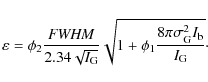
Aims. We investigate the astrometric performance of the FORS1 and FORS2 cameras of the VLT at long time scales with emphasis on systematic errors which normally prevent attaining a precision better than 1 mas.
Methods. The study is based on multi-epoch time series of observations of a single sky region imaged with a time spacing of 2-6 years at FORS1 and 1-5 months at FORS2. Images were processed with a technique that reduces atmospheric image motion, geometric distortions, and takes into account relative displacement of reference stars in time.
Results. We performed a detailed analysis of a random error of positions that was shown to be dominated by the uncertainty of the star photocenter determination. The component of the random error corresponding to image motion was found to be caused primarily by optical aberrations and variations of atmospheric PSF size but not by the effect of atmospheric image motion. Comparison of observed and model annual/monthly epoch average positions yielded estimates of systematic errors for which temporal properties and distribution in the CCD plane are given. At frame center, the systematic component is about 25 as. Systematic errors are shown to be caused mainly by a combined effect of the image asymmetry and seeing variations which therefore should be strongly limited to avoid generating random and systematic errors. For a series of 30 images, we demonstrated presicion of about 50 as stable on daily, monthly, and annual time scales. Small systematic errors and a Gaussian distribution of positional residuals at any time scale indicate that the astrometric accuracy of the VLT is comparable to the precision. Relative proper motion and trigonometric parallaxes of stars in the center of the test field were derived with a precision of 20 as yr^-1 and 40 as for 17-19 mag stars. Therefore, distances at 1 kpc could be determinable at a 4% precision if suitably distant reference objects are in the field.
Conclusions. We prove that the VLT with FORS1/2 cameras are not subject to significant systematic errors at time scales from a few hours to a few years providing that observations are obtained in narrow seeing limits. The astrometric performance of the VLT imaging cameras meets requirements necessary for many astrophysical applications, in particular, exoplanet studies and determination of relative trigonometric distances by ensuring a high accuracy of observations, at least 50 as attained for image series of 0.5 hour.

Key words: astrometry - atmospheric effects - instrumentation: high angular resolution - planetary systems

1 Introduction

The availability of astrometric measurements of proper motion and parallactic displacements at 10-100 microarsec precision provide a base for many astrophysical applications, e.g. determination of the distances to stars and their absolute luminosity, detection of planets, microlensing studies of the mass distribution in the Galaxy, dynamics of the Galaxy Center stars, etc.

The above studies imply use of very high precision astrometry, requiring both reduction methods that are fairly insensitive to major noise sources as well as telescopes fulfilling the precision requirements and temporal stability. The availability of suitable instruments however hardly matches current demand, and is in large disproportion to envisioned future endeavors. In particular, this hinders programmes studying exoplanet populations by means of astrometry, which would powerfully extend and complement efforts based on other techniques and provide an efficient pathway towards identifying habitable planets.

The best future prospects for high-precision astrometry can be expected from space telescopes, but the only mission currently planned is GAIA (Perryman et al. 2001). Achieving a single-measurement precision below 10 as on V < 13 stars, it will offer the opportunity to discover and study several thousands of planets (Casertano et al. 2008). However, GAIA operates as an all-sky survey and cannot be pointed to a specific target, and its accuracy degrades rapidly towards fainter stars (Lindegren et al. 2007).

In contrast, pointing to selected targets is possible with ground-based telescopes, effectively measuring distances in binary star systems by means of optical interferometry. These achieve accuracies of the order of those of GAIA at V > 15. VLTI/PRIMA is able to measure distances between stars separated by 10 with 10 as precision (Delplancke et al. 2000) with a 30 min integration time; at a similar 20 as h^-1 precision, star separations can be measured with the Keck Interferometer (Boden et al. 1999). Moreover, at 30 separation in pairs of bright stars, an astrometric precision of 100 as has been achieved by Lane et al. (2000) with the Palomar Testbed Interferometer (PTI), and Lane & Muterspagh (2004) and Muterspagh et al. (2006) reported an accuracy of 20 as stable over a few nights. The availability of and access to ground-based high-precision astrometry facilities is however extremely limited, so that no exoplanet detection programme has yet been established.

Large ground-based monopupil telescopes that operates in imaging mode also can significantly contribute to the detection and measurement planetary systems. Unlike infrared interferometers, these telescopes measure the position of a target either with reference to a single star or to a grid of reference stars. For a long time, however, astrometric measurements with ground-based imaging telescopes were believed to be limited by about 1 mas precision due to atmospheric image motion (Lindegren 1980). This limitation, however, is not fundamental and rather reflects the performance of the conventional astrometric technique. The first high precision observations well below 1 mas were obtained by Pravdo & Shaklan (1996) at the Hale telescope with a D=5 m aperture. In the field of 90 , they demonstrated precision of 150 as h^-1. This precision was further improved by Cameron et al. (2008) with the use of adaptive optics. They reached a precision of 100 as with a 2 min exposure and showed it to be stable over 2 months.

A detailed analysis of the process of differential measurements affected by image motion allowed Lazorenko & Lazorenko (2004) to show that the excellent results obtained by Pravdo & Shaklan (1996) represent the actual astrometric performance of large telescopes. It was shown that angular observations with very large monopupil telescopes are not atmosphere limited due to effective averaging of phase distortions over the aperture. For observations in very narrow fields, atmospheric image motion decreases as D^-3/2 (Lazorenko 2002) reaching below other error components. Also, the image motion spectrum can be further filtered in the process of the reduction by using reference field stars as a specific filter. Astrometric precision greatly benefits from the use of large  m apertures.

Besides atmospheric image motion, one can list a number of other systematic and random error sources that could prevent us to reach a as level of the precision. Many sources of error depend on the telescope and cause long-term astrometric instability of results. To ascertain the practical feasibility of this new astrometric method, we have chosen the high performance FORS1/2 cameras set at the VLT with excellent seeing. We have undertaken several tests of various time scales, ranging from a few hours to several years.

The first test (Lazorenko 2006) was based on a single four-hour series of FORS2 images in Galactic Bulge obtained by Moutou et al. (2003). It proved the validity of the basic concept of the new astrometric method and an astrometric precision of 300 as with a 17 s exposure was reached.

In the second test (Lazorenko et al. 2007), we investigated the astrometric precision of the FORS1 camera over time scales of a few days. For this study we used the two-epoch (2000 and 2002) image series (Motch et al. 2003), each epoch represented by four consecutive nights. We reached a positional precision of  as and detected no instrumental systematic errors above 30 as at the time scales considered. The precision of a series of n images was shown to improve as at least to n = 30, which corresponds to a 40-50 as astrometric precision.

This paper concludes our study of the VLT camera astrometric performance and extends our previous short time scale results to intervals of 1-5 months and 2-6 years. This covers all time scales required for typical microlensing, exoplanet search applications, and Galaxy kinematics studies. In Sect. 2 we outline the strategy of this study, observations, and the computation of the star image photocenters. Astrometric reduction based on the reduction model (Sect. 3) is described in Sect. 4. The random errors of single measurements are analyzed in Sect. 5, where we extract the image motion component, which proved to be of instrumental origin. Systematic errors in epoch monthly/annual average positions, and their spatial and temporal properties are considered in Sect. 6. Astrometric precision in terms of the Allan deviation is discussed in Sect. 7.

2 Observation strategy and computation of photocenters

As a test star field, the best choice is the field near the neutron star RX J0720.4-3125 whose FORS1/UT1 images of  angular size obtained in Dec. 2000 and Dec. 2002 by Motch et al. (2003) were already used in our previous study (Lazorenko et al. 2007). Its uniqueness is that it has the best history of observations available in the ESO/ST ECF Archives suitable for precision astrometry. Data are represented by 65 images obtained with the B filter and obtained with a 2 year epoch difference, which allows for a reduction with no bias due to parallax. Also, the field is densely populated, containing about 200 stars with a high light signal. We repeatedly observed it in Dec 2006, at integer differences of years, with FORS1/UT2 (1 px =0.10 scale) and the same B filter, thus comparing model predicted and observed positions at three annual epochs, verifying the very long-term astrometric stability of the VLT at 2-6 years, and computing relative proper motions used later on for the reduction of FORS2 data. Observations were performed with the LADC optical system (Avila et al. 1997) that improves image quality by compensating for the differential chromatic refraction (DCR) of the atmosphere.

The same test star field was imaged five times at FORS2 (1 px =0.126 scale) with the filter with a T=70 s exposure to keep star fluxes at approximately the same level as in the FORS1 images. A one month spacing between time series was chosen to match the typical sampling for the observation of astrometric microlensing or of the astrometric shift of stars caused by an orbiting planet. The availability of FORS1 images gives us an opportunity to correct the measured FORS2 positions for highly accurate relative proper motions determined at six year time intervals. This correction is critically important since elimination of proper motion from FORS2 positions decreases the number of model parameters, thus greatly improving the reliability of the subsequent statistical analysis. After elimination of proper motion obtained as shown, the positions of 5 series are reduced to a common standard frame with a model that fits star motion by parallax. Residuals of star positions (measured minus model) are then analyzed to detect systematic errors and any correlations with time or magnitude. A summary of observation data is given in Table 1. Note the large variations of seeing which does not favor high precision astrometry (Sect. 6).

The primary goal of this study is the investigation of random and systematic positional errors of the FORS cameras. This task requires a careful reduction of observations, including determination of proper motion and parallaxes with the combined use of images obtained with two cameras. We aim to demonstrate that a 300 as single measurement precision of narrow-field astrometry translates to about 50 as precision for a series of 30 measurements.

Table 1:   Summary of the test field observations.

Raw images were calibrated (debiased and flat-fielded) using calibration master files. Star images having even a single saturated pixel were marked and rejected for a loss, even small, of positional information. Positions of star photocenters X,Y were computed with the profile fitting technique based on the 12-parameter model specific for the VLT images (Lazorenko 2006). By careful examination, we developed a three component model that fits observed profiles to the photon noise limit. The dominant model component that approximates the core of the PSF (point spread function) is a relatively compact Gaussian with width parameters , along x,y axes and a flux containing 2/3 of the total star flux I. Two auxiliary Gaussians, each one multiplied by a factor x² or y², are co-centered at the dominant component and approximate wings of the PSF. The model also takes into account the high-frequency oscillating feature of the PSF, computing it as a systematic discrepancy between the model and observed star profiles. Deviations between the model and observed pixel counts were found to be at the level. Determination of star photocenters is a very important element of the process because, as we show later on, most of the random and systematic errors occur at this phase.

The precision of the star photocenter was estimated by numerical simulation of random images yielding an expression similar to that derived by Irwin (1985) for a single Gaussian profile

This equation is valid in a much wider range of fluxes, seeing, and background signal as compared to our former expression (Lazorenko et al. 2007). Here fluxes are given in electrons, is expressed in pixels, and are empiric factors, and is a relation valid for the VLT images. Due to the complex star profiles, coefficients  and  are not units, in which case Eq. (1) transforms to the expression given by Irwin (1985).

Computed model parameters were analyzed to detect and reject non-standardly shaped images indicating computation errors and actual image defects caused by blending, cosmic rays, etc. All images with model parameters and exceeding some deliberately set thresholds were discarded. Thresholds were chosen so that the frequency of rejections was about 1% for bright images. At this fixed threshold, the number of rejections gradually increased with magnitude, reaching 10-25% for faint images, which are more sensitive to the background irregularities. In contrast, filtration based on caused excessive rejection of the brightest images, since the accuracy of the model profile is insufficient at high light signals and becomes comparable to the statistical fluctuations of counts. This gives rise to a with subsequent false rejection of measurements.

Most often, discarded faint star images have excessive size. This produced a selective effect seen as a systematic dependence of image parameters on flux I. A difference between the mean image size parameter in the filted star sample and its mean value in the initial star sample is typical. The systematic dependence of the ratio on flux is shown in Fig. 1. While no difference is seen for bright images, at the faint end the size of stars selected for further processing is systematically 10-30% smaller. For FORS1 images the effect is stronger due to the larger pixel scale (lower signal to noise ratio) and many cosmic rays occured over the long integration time. The selection described here induces a similar dependence of the centroiding error on flux (Sect. 5).

Further astrometric reduction revealed that some stars show a significant correlation between model minus observed residuals of positions and variations of seeing. This effect, detected primarily for relatively close star pairs, is due to the asymmetry of images caused by the light from the nearby star (see Sect. 6). About 1% of measurements subject to this effect were rejected.

3 Astrometric reduction model

is a sample of stars imaged fold in the sky area of angular radius Rcentered on a target star which we denote with a subscript i=0. In general, may represent only a portion of the complete sample of stars seen in the telescope FoV. Given the measured star centroids X_im, Y_im, we derive, on each CCD image, the differential position of the target, its relative parallax, proper motion, and deviations V_im from the model that may hide the astrometric signal (e.g. planetary signature). These quantities are not measured directly and are rather estimates of model parameters found in a certain reference system set by the reduction model; therefore, they depend on it. The image m=0 sets the zero-point of positions, a grid of reference stars in this image defines the reference frame. For processing therefore we use relative CCD positions x_im=X_im-X_i0, y_im=Y_im-Y_i0.

The certain difficulty for astrometric processing is brought by the instability of the reference frame in time due to the atmospheric differential chromatism (e.g. Monet et al. 1992; Pravdo & Shaklan 1996; Lazorenko 2006; Lazorenko et al. 2007), variable geometric distortion, proper motions, etc. In our previous study (Lazorenko et al. 2007), we developed a model that correctly handles this problem and ensures a solution in a uniform system with no distinction between target and reference stars. Here we propose a more general solution that allows an easy readjustment of the system of model parameters and of deviations V_im in a way that is optimal for a particular study. The model deals with atmospheric image motion (Sect. 3.1), geometric distortions (Sect. 3.2), and instability of the reference frame in time (Sect. 3.3). We emphasize that all the data derived from the differential reduction (proper motions, parallaxes, chromatic parameters, etc.) are intrinsically relative (not absolute). This point is discussed in detail in Sect. 3.5.

3.1 Atmospheric image motion

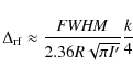
The variance of the atmospheric image motion in positions measured in narrow fields is given by Lindegren's (1980) expression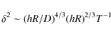

where h is the altitude of the atmospheric turbulent layer generating the image motion and R is a star configuration angular size. For a binary star, R is the star separation. Equation (2) refers to the very narrow angle observations defined by condition

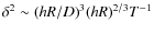
otherwise we have the much worse . Equation (2) predicts a weak improvement of with Dthus limiting ground-based observations to a few milliarcsec precision at reasonable R and T. For a fictitious case of symmetric continuous distribution of reference stars around a target in a circle of a radius R, Lindegren obtained with a stronger dependence on D. However, no way to practically implement potentially useful symmetric distributions was found, thus current estimates of are based on Eq. (2) with milliarcsec limitation.

We have shown (Lazorenko 2002; Lazorenko & Lazorenko 2004) that

• any arbitrary discrete reference star distribution, of at least three stars, can be symmetrized;
• symmetrization is always implemented by a standard plate reduction with a linear or more complex model;
• , which suggests faster improvement of with D in comparison to Lindegren's prediction for symmetric continuous distributions;
• use of a large  m is required to meet condition (3) for high stratospheric layers.

Here we briefly summarize the concept of image motion reduction based on the spectral description of this process. We have shown that the spectral power density G (q) of differential image motion in the domain of spatial frequencies q related to the turbulent layer is the product of two factors. The first factor F'(q) depends on D, the altitude h and properties of the atmospheric turbulent layer generating the image motion, and exposure time T. The second factor F'' depends only on the way we define the ``differential position'' and on the geometry of reference star distribution relative to the target. This factor is expanded in a series of even powers of q. Hence G(q) has a simple modal structure with terms F''_2s dependent on the distribution of stars on the sky only. Integration of the power density over q yields the variance of differential image motion

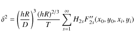
that inherits the initial modal structure of G(q), and H_2s are modal coefficients. Of course, the actual value of is the sum over all turbulent layers with h ranging from a few to 25 km. The factor (hR/D)³ shows that large telescopes easily suppress even high stratospheric turbulence. Equation (4) however is valid only for observations at narrow angles (3). In the case of the VLT, it holds only approximately at , which causes a problem of a lack of reference stars. With D<8 m apertures, only low-layer turbulence is well reduced, resulting in a moderate suppression of the image motion.

For optical interferometers, the atmospheric noise decreases as d^-2/3 (Shao & Colavita 1992) and phase fluctuations are mitigated by probing the difference of phase at ends of the instrument long baseline d. For monopupil telescopes, a fast decrease of image motion occurs in another way, by averaging the turbulent phase fluctuations over the aperture. The efficiency of phase averaging depends on the symmetry of the star configuration, which requires availability of the grid of reference stars. We emphasize that, unlike optical interferometers, monopupil telescopes are not adapted for precision measurement of the angular offset between a pair of stars due to the intrinsic asymmetry of this star configuration, for which follows dependence (2).

From Eq. (4) it follows that can be reduced by removing (filtering) the several first most significant modes up to some optional k/2 spectral mode. The residual variance obtained in this way depends on the first high k=2s (k is even integer) active mode of the image motion spectrum and is therefore of a comparatively small magnitude. For the VLT, the gain in is a factor of 100 and more. The above possibility follows from the next considerations: the relative position of the target in image m along the x axis (here and farther on we omit similar expressions for y) is defined by the quantity

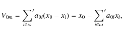
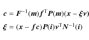
where prime indicates that index i=0 is omitted. Coefficients a_0i meet the normalizing condition and are specified below. Image motion in V is described by Eq. (4) with where g_ws are constants and f_iw are values of functions f_w for a star i. Here f_w are basic functions numbered with an index defined in Cartesian coordinates of the reference frame and formed with successive integer powers of the coordinates: . Thus for i star. The expression for F''_2s that refers to some mode sinvolves only polynomials of x,y with a sum of powers equal to s. Indices w run from w₁=s(s+1)/2+1 to w₂=(s+1)(s+2)/2. The quadratic structure of the expression for F''_2s implies that the s mode is zero when coefficients a_0i meet conditions

for each basic function. Evidently, all modes up to s=k/2 -1 vanish if a_0i satisfy Eqs. (6) for each s<k/2. For that reason, a_0i are found as a solution of a linear system of

Equations (6). Solution of this redundant system (because usually N>N') is found with a supplementary condition

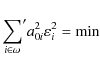
set on the variance of the second item in (5) caused by centroiding errors for reference stars. For dense sky star areas the approximate expression

is valid where I' is the light flux per unit area coming from bright reference stars.

Thus, the quantity V defined by (5) is free from the first modes of the image motion spectrum untill k/2 providing that a_0i confirm to Eqs. (6), (8). The variance of V is

Because due to (4), and according to Eq. (9), the value of is minimum at

which is reached at some optimal size (see Table 2) of the reference frame .

3.2 Single plate reduction

A standard plate reduction produces effects equivalent to symmetrization of the reference frame (Lazorenko & Lazorenko 2004). Really, the basic equation of the plate model, in vector representation, is

where is a vector of x positions (including target), is a matrix formed by vectors f_iw, and is a vector of N' model parameters c_w. We require that N' takes only those discrete values which are defined by (7) for some optional k(k=4 and N'=3 corresponds to the linear model, k=6 and N'=6 refer to the model that includes quadratic powers of x,y, etc). The least square solution of (12) is where is the normal matrix and is the diagonal matrix of weights P assigned differently for the target and reference stars. To comply with the image motion reduction procedure, we set

considering that is the effective variance of measurements. The best estimate of the vector is where is a projective matrix that maps the matrix to itself:

Residuals of the least square fit is the vector , or

with the property

The covariance matrix of is where curly brackets designate mathematical expectation. Using Eq. (15) and considering that , we find where is a diagonal matrix of elements . Diagonal ii elements of are a variance of the residuals V_i. For target (P₀ = 0), all elements in column i=0 of are zero. Hence which is equivalent to Eq. (10) where

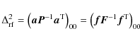
defines the variance of reference frame component at the location of the target. For reference star i we come to a different expression

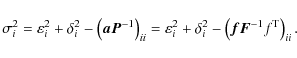
The last term is the noise from the reference frame and is a composition of two components, noise from the star i itself with the variance , and nearby star grid noise with the variance defined by Eq. (17) at the location of star i. Adding their inverse as weights, we find . Hence

Equations (15), (14) of the plate model correspond to Eqs. (5), (6) of the image motion filtration and (8) is the least square condition. Therefore both methods are equivalent. However, we imply that the model (12) should include a sequence of all basic functions f_w with no omission and at least k=4 (linear plate solution) or above is chosen. The use of higher-order models results in better filtration of image motion, though, as follows from Eq. (9), it increases . In the special case of k=2, differential positions are measured relative to the centroid of the reference stars; this should be avoided since it corrupts the symmetry of the reference configuration and greatly amplifies image motion to set by (2).

3.3 Multi-plate reduction

A single plate model (12) is easily extended to the case of multiple  images. For this purpose we specify, for any star i, a set of  model parameters which are zero-points, relative proper motion and , relative parallax , etc. Thus the position x_im of any star i in image m is modelled by where are functions of time (of image number) coupled to and c_wm are model parameters c_w in image m. Using matrices similar to the above quantities, we reach

in a concatenated space formed by two types of basic functions, f and , related to the spatial coordinates or to time respectively. A similar expression is written for y, which requires introduction of the corresponding matrix.

Equation (20) is a set of equations solvable by the least square fit with respect to parameters c_wm and parameters . Also, for each image m, we introduce an weight matrix with elements used for the reduction in x, y space and treated like the matrix of Sect. 3.2. Another diagonal matrix related to a star i takes into account the change in time of the residuals . Diagonal elements of are equal to defined by Eqs. (10) or (19) depending on the star type. When star i measurements are unavailable at image m, the corresponding elements of matrices  and are put to zero.

Direct solution of system (20) is, however, impossible due to the ambiguity between and . If some component s of parameters (for example, proper motion) systematically changes across the CCD, this change can be fitted by a polynomial and thus is not resolvable from a change in c_wm. And vice versa, a change in time of some component w of c_wm produces an effect that is similar to a change in . Therefore Eq. 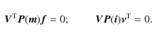(20) is solved under conditions

where is the diagonal matrix of weights . For reference stars, are arbitrary (e.g. average of P_im over all measurements) while for the target. The least square estimates and of Eq. (20) are found from the system of equations

solved iteratively using reference stars only with no contribution from the target due to zero weights P_0m and . Above, is a normal matrix for a star i in vector space and is a matrix related to image m. For simplicity, in Eq. (22) we omit expressions related to y.

A simple, non-iterative solution of Eq. (22) exists, requiring only that each star measurement is available at each image, at constant flux and seeing conditions. In this case and therefore and providing that is set.

Given solution and , we derive residuals

which are orthogonal to the basic vectors (at each m) and (for each i):

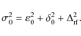
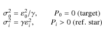
Putting solution derived from measurements of reference stars only into the second equation of (22), we find parameters of the target. Hence, the variance of V at image m is

3.4 Reference frame quality

In very dense reference frames, astrometric precision is limited only by errors of the photocenter determination if image motion is well reduced. For sparsely populated reference frames, the noise degrades the astrometric precision. This takes place even in our case of relatively low galactic latitude, -8. Figure 2 shows the distribution of computed for each star (processed as a target) and each FORS1 image as a function of star distance r from the frame center. The vertical scatter of dots for each star is rather large and is caused by variations of seeing and background. At frame center, is minimum, about 150 as in average observing conditions. Although small, it is comparable to the centroiding error,  as, of the brightest targets. A good indicator of the ability of the reference frame to keep the output error of positions near to the precision of image centroiding is the quantity

which depends on the star location in the frame, its brightness, and in extreme cases of ratio, it varies from zero to a unit value. In terms of , the dependence of on the reference frame noise given by Eqs. (10) and (19) is

where for simplicity we assumed . Although written for a single image only, the above equations emphasize the problem caused by sparse reference frames with small . Note that a decrease in with for reference stars does not improve the signal-to-noise ratio (see Sect.3.5).

Figure 2 shows distribution of as a function of magnitude for each star processed as a target. The dependence has a specific decline at the bright end, to . For bright targets even at field center due to the limited number of reference stars. It follows that for small , the resulting variance significantly exceeds the centroiding error since . In this respect, is a factor that specifies the quality of the reference frame.

3.5 System of output data

Due to the differential reduction, the computed parameters and positional residuals V are relative. Weights define the system of parameters of both target and reference stars. It follows from Eq. (21) which allows interpretation of as the residual of the least square fit of some absolute parameters by basic functions f. Therefore what we measure are not but relative values

where is a projective matrix defined similarly to but with weights put instead of P, and is a least-square polynomial fit of over reference stars in . Thus the reference frame  and system weights fully define rule (28) of transformation to at k (or N'). Recall that weights for reference stars are arbitrary and thus so is the transformation (28). From general considerations we assume that are equal to P_im averaged over m, and .

Noting the similar structure of Eqs. (21) and (24) (the first equation), we can apply the above considerations to the system of residuals V and find that it is defined by weights P_im. Residuals V are related to some ``absolute'' residuals by the expression of (28) as

There is however an essential difference in treating Eqs. (28) and (29). The variance of depends primarily on the centroiding error while the scatter of is caused by the actual dispersion of star parameters (e.g. proper motions) within and can largely exceed random errors. Therefore, comparison of values computed with different k, R or , will show a divergence dependent on the particular spatial distribution and the dispersion of . For example, the estimates of parallaxes computed in this test field for the same target, but with different k and , are scattered with a standard deviation of about as independent of the target brightness, which exceeds the errors of parallax determination. This is quite normal and mirrors the change of reference system. Therefore, estimates of obtained in different systems not can be merged into a single system, which will produce meaningless result. Unlike this, the change of reference system affects V very much less (by an order) which proves their merging into a single ``system'' (Sect. 4.3).

System weights P_im and essentially affect output residuals V and model parameters , which is better analyzed from the point of view of signal detection. is a signal in x that generates some response z' in V. With regard to the target, the amplitude of z', according to Eq. (15), is since a_i0=0. With Eq. (27) defining the variance of V₀, we find that the signal-to-noise ratio is . Thus, while the measured signal z in V₀ is independent of properties of the reference field, the signal-to-noise degrades at low , primarily for bright targets. Now consider the reference star i. In this case according to Eq. (15). From Eq. (18) and the definition of we find hence and . We conclude that the signal-to-noise ratio is equal for either type of stars, but the best 100% response z' in V is detected for targets. For reference stars, the signal decreases as , especially significant for bright stars.

For some specific studies dealing with a full sample of stars (kinematics of open cluster members), uniformity of the system of output model parameters is much desired. In this case, the best way is to process all stars as reference objects ( , ). The model solution is then related to via Eq. (28). With respect to proper motions, this transformation is where corresponds to the system of weights .

Untill now we have discussed reduction with reference to a star grid within a single isolated circular area disregarding other stars in the FoV. In our previous study (Lazorenko et al. 2007), we considered reduction with multiple overlapping reference subframes each centered at each i star seen in the FoV. In this approach, the star i is processed, at first, as a target (P_i=0) measured with reference to its own local subframe . At the same time, this star is a reference object ( ) for adjacent subframes. The solution initially related to local frames is iteratively expanded to a reference grid  (all FoV) and a single common system by applying a set of interlinking Eqs. (21). It can be shown that the final solution in does not depend on the size of the initial frames . Residuals V of this solution in each image m meet conditions . These conditions correspond to Eq. (24) for reference stars in providing that . Therefore a solution with overlapping reference subframes is equivalent to that in a single isolated area , or to a standard solution performed with all stars used as reference only. Consequently, no improvement in the signal to noise ratio is expected. This version of the reduction is useful for a low number of model parameters (vector is not used in the model), high uniformity of model parameters and residuals V, and a fast convergence of iterations. However, assumption  used here means that P_im is constant in time, which is not always acceptable.

For this study, we used standard reduction (Sect. 3.3) computing the target position with weights P₀=0, to ensure the best response to systematic errors in V.

Table 2:   Minimum and optimal radii of reference fields.

4 Astrometric data reduction

4.1 Reduction of FORS1 images

One of the FORS1 sky images obtained in Dec. 2000 at a seeing near its mean level was used as a reference. Photocenters were computed for 180 stars of B=18-24 mag in the central area. Reductions were performed with a standard model (Sect. 3.3) that yields residuals V and model parameters of a target star i relative to the local grid of reference stars . Due to the extremely small value of systematic errors, we tried to improve the statistics by accumulating data over all stars available. Therefore, reductions were repeated 180 times, processing each star iin turn, as a target (which till now was denoted by a subscript i=0). For that reason, the astrometric precision varied depending on the distance r of the star i from the frame center. For the brightest stars, this occurred due to decreasing from at the frame center to 0.2 at the periphery (Fig. 2) with a corresponding error increase by 25-50%. Computations were carried out with all k from 6 to 16 and all R from some (Table 2) that provides the minimum number of reference stars needed at a given k, to the maximum . The first run was performed with zero image motion and afterwards computations were repeated with the actual estimate of (Sect. 5).

We assumed a 10-parameter model for with zero-points, proper motions , , atmospheric differential chromatic parameter , the LADC compensating displacement , and with no parallax for integer year differences between epochs. Four extra g_xx, g_xy, g_yx, and g_yy model terms for each star were applied to compensate for a strong, over 200 px jittering of images. Jittering induced a large signal in V, clearly correlated with telescope displacement , along the x, y axes. This effect increased with R, reaching several milliarcseconds at , . The jittering makes the reduction difficult, and is the reason that we discarded a linear (k=4) model reduction.

Jittering moves the star field with reference to the camera optics. This causes a change in the optical distortion (say along x) at some point x,y from its initial value to . A similar expression is valid for the distortion along the y axis. Naming the partial derivatives used here as g_**, we come to the expression

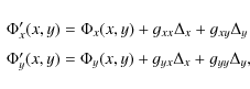
equally applicable for the correction of positions. Assuming that optical distortions are stable over the observing period, g_** terms are included in, and found as components of .

An example of the measured and model star motion over the CCD surface is shown in Fig. 3 for a red (B=20.8, B-R=2.8) star with proper motion  mas yr^-1,  mas yr^-1, and trigonometric parallax (all relative)  mas which was computed later based on FORS2 images (Sect. 4.2). This graph is actually rather simplified because it refers to positions corrected for polynomial and for jitter related terms. The intricate shape of the track is due mainly to the DCR shift of images within a single series. In the blue band, this motion exceeds 10 mas while in the red filter the effect is an order lower. This makes it clear, for instance, why reference star displacements should be taken into account when processing B images.

The dependence on magnitude of the internal precision of proper motions is shown in Fig. 4. These estimates correspond to the formal least squares precision and take into account components , , and of the total random error . Due to the large time span between epochs, proper motions were derived with high precision, reaching 20 as yr^-1 for bright stars. Systematic errors (Sect. 6) degrade precision little since their contribution is small in comparison to random errors (see Sect. 4.2).

4.2 Reduction of FORS2 images based on FORS1 proper motions

For processing of FORS2 images we used high-precision proper motions derived from the reduction of FORS1 images on a six year time base. At five-month spacing, they ensure very accurate corrections. The possibility to use proper motions that fit image measurements of the other camera, different wavelength, and at distant epochs, however, is not evident and should be used with care. On the other hand, the precision of FORS2 positions obtained in this way is an indicator of the actual accuracy of FORS1 proper motions. Most important, the elimination of proper motions from model parameters essentially increases the DoF (degrees of freedom) of least square residuals in temporal subspace thus making further study of systematic errors more reliable.

The reduction was started by finding the FORS2 image obtained at normal seeing and best matching the star content of FORS1 images. This image at epoch T₀was used as a reference for the reduction of all FORS2 images. In most cases, the difference in star content from the two cameras occured for a small gap between two CCD chips of FORS2 and saturation of bright stars in the R filter. In this way, 152 common stars were selected for further reduction, which started from applying corrections for proper motion occuring in star positions between epochs T₀and T_m. This was performed taking into account the singularity of astrometric reduction according to which the i-th target position (and proper motion ) is related to a particular subset of reference stars , whose unique model parameters (denoted by in contrast to ) are valid within this subset only. Therefore, to conserve the reference system, a reduction of FORS2 images for a target i was performed with reference to the same frame as used for FORS1. Also, we applied weights that are same as those involved in the reduction of FORS1 images, that is, using average light fluxes in the blue filter. Thus, each reference (with respect to target i) star positions were corrected by

This complicated procedure is due to the necessity to conserve the system of model parameters when processing different sets of images. Violation of this principle immediately destroys the accuracy. Thus, direct application of corrections to all measurements of reference stars in is incorrect because these are related to their own frames which differ from . Mismatch of these areas and even a small inconsistency of the reference star ensemble sometimes result in large 1000-5000 as epoch residuals. Even use of proper motions did not ensure complete identity of related to each camera due to inavailability of some FORS1 stars in FORS2 images.

The reduction model included zero-points, chromatic parameters , , and trigonometric parallaxes . Formal random precision of FORS2 parallaxes for stars of different brightness is given by Fig. 4. For the best stars, relative parallaxes are determined with a precision near to 40 as, which means that distances at 1 kpc are measurable with a 4% precision. A few large upward deviations in Fig. 4 for some stars are caused by a low number of measurements (oversaturation of bright images, or position in the gap between two chips of the camera) or by the peripheral position of stars and thus low (large ).

The precision of parallaxes is increased by use of FORS1 proper motions, allowing us to exclude a component from model parameters , removing in this way a strong correlation between and . In other cases, the expected precision of parallaxes from the 5-month series of observations is 200 as only.

Systematic errors, of course, affect the accuracy of both proper motion and parallax determination. In Sect.6 we show that the systematic error for targets near frame center is about 25 as, or a half of the random error of epoch average positions for bright stars, at months to year time scales. Translating this estimate to parallaxes, we find that systematic errors contribute approximately 20 as to each star parallax and 10 as yr^-1 to proper motions irrespective of the star magnitude.

4.3 Merged residuals

While processing, we computed residuals V for each star i, each image m, all reduction modes k from 6 to 16, and several reference field sizes R, including . The best precision residuals computed at we denote as V_im(k). In practice, however, we do not require multiply defined residuals but rather a single set of residuals which for a particular star i is the best estimate of the planetary signal at the moment of image m exposure. For that purpose we merge V_im(k) into a single system, the possibility of which follows from the discussion in Sect. 3.5.

Let us consider Fig. 5 that presents an example of the image-to-image change of V_im(k) computed with different k for two stars of different brightness. Residuals corresponding to different k are seen to be highly correlated, especially for a faint star, and fluctuate near their average, being a function of m. Recall that according to (29), where a_ij(k) refer to k used. Therefore where is an average of a_ij(k) with respect to k. Hence . The variance of this difference, neglecting the second term, is , or at k given. Thus, the standard deviation of depends on almost linearly. This approximation is confirmed by actual data, as shown in Fig. 6.

Given 6 sets of V_im(k) corresponding to k=6...16 for each target i, we merged them into the weighted average using weights . Along with V, merged residuals were tested for the presence of systematic errors (Sect. 6). As explained in Sect. 3.5, the merging is not applicable to model parameters .

For faint stars, the relative amplitude of V fluctuations near is insignificant (Fig. 5a) since . Therefore at any k and the use of instead of V is of low efficiency. For bright stars (Fig. 5b), the precision of is better due to the averaging of the reference frame noise.

5 Random errors

5.1 Calibration of the image centroiding error dependence on flux

In this section, our study was carried out with images obtained in a narrow seeing range of 0.47-0.78 , which includes almost all FORS1 and about 80% of FORS2 images. The use of images out of this range leads to a noticeable increase of random errors.

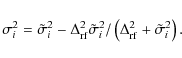
The use of stars of different brightness to investigate systematic errors requires careful calibration of the dependence on flux of the image centroiding error (1). For calibration purposes, the best residuals are V computed at the minimum possible (Table 2) since they contain negligible input of atmospheric image motion . Using the variance of residuals V computed for each k at , we can find the residual discrepancy of the decomposition (25) into error components

for each target i. The change of this quantity with star magnitude is shown in Fig. 7 by dashed lines for each k. All curves corresponding to different k modes closely follow a common dependence with little scatter. The anomalously large deviation seen for the FORS1 camera at k=6 originates from the large jittering of images which was not completely compensated by the reduction. For high k modes this effect is well removed. While for bright stars, discrepancies are fairly small, at the faint end we note a systematic negative bias caused by incorrect modelling of errors. This bias almost does not depend on k and is approximately proportional to  . Therefore we assumed that this discrepancy is caused by insufficient validity of model (1) for  , which requires an additive correction  with a coefficient  independent of flux. A similar correction should be applied to  also. Correction factors  to and computed in 0.5 mag flux bins are shown in Fig. 8 as a function of magnitude.

A change of with brightness in Fig. 8 is similar for both cameras. A negative trend over a 4-5 mag range of brightness reproduces the dependence of star image size on flux (Fig. 1) and therefore probably is a consequence of selective filtration based on star profile parameters when star images with excessive size were discarded (Sect. 2). The use of more compact images in comparison to the initial star sample, of course, results in an improvement of the effective centroiding error observed in Fig. 8. A similar improvement of precision for the brightest images occurs for the selection based on criterion (Sect. 2).

Averaging with respect to k produced final estimates shown in Fig. 8 by solid lines. With these corrections, residuals (32) have been recomputed yielding new discrepancies with much smaller magnitudes (Fig. 7, solid lines). Having found the calibration factor , we can correctly estimate  at any  simply by adding the image motion variance :

The term is used to take into account the dependence of on flux which originally was considered constant. This also compensates, at least statistically, the use of a single correction factor for both and .

The validity of above calibration is illustrated in Fig. 9 where we compare the astrometric precision of a single photocenter measurement restored from observations with its model prediction in the case of reductions with R=1.5 and k=10. The measured astrometric precision, for each star, was computed based on the observed variance of V (mean in x and y), derived in Sect. 5.2, and representation (33). These results, as for model values for each target, were averaged over all data available. Figure 9 shows a good match of the observed and model precision over wide range of magnitudes. This graph matches well our previous results for FORS1 based on a reduction technique with overlapping reference frames (Lazorenko et al. 2007).

We emphasize that both and are estimates of the actual precision of the photocenter determination. The difference is that the first one refers to the star sample affected by selection while is related to the imaginary sample of FORS images with no defects. In spite of the small value of , the subsequent study of image motion and systematic errors greatly favours its use since it allows us to incorporate large amount of data from faint stars.

5.2 Image motion

Taking advantage of the availability of a well calibrated image centroiding error, we used Eq. (33) to extract the image motion component at various R. This equation was solved numerically for each star taking into consideration the fact that the reference frame noise is a function of and . The results averaged over all stars available and computed for each kand R are shown in Fig. 10. Comparing estimates obtained for both cameras, one may note the similarity of results in spite of the difference in pixel scale, number and spacing of epochs, different reduction model parameters, different method of reduction and, especially, an 8-fold difference in exposure T (600 and 70 s for FORS1 and FORS2 respectively). The last aspect raises a doubt about the validity of relating the measured image motion to atmospheric turbulence.

At each fixed k, estimates were fitted by a power law

assuming that R is given in minutes of arc. Fitting parameters B and b are given in Table 3 for the first few k modes only since the results for k>12 are too uncertain. Excessive estimates of B (in comparison to FORS2) found at k=6 and k=8 could be due to the residual effect of large image jittering of FORS1 images. For comparison, the table contains and coefficients of Eq. (34) expected for differential image motion caused by atmospheric turbulence. These values were obtained by scaling model coefficients (Lazorenko & Lazorenko 2004) that refer to typical atmospheric conditions at Chilean observatories, to current exposures and telescope aperture. The atmospheric-related amplitude is much smaller than the observed one, especially for FORS1 with a 3-8 fold discrepancy. Such a large difference suggests that we are measuring an effect not related to the atmospheric turbulence.

In a pilot study of FORS2 astrometric performance, Lazorenko (2006) estimated Eq. (34) parameters B' and b'using a single night observation series with T=17 s exposure. Coefficients B' reproduced in Table 3 are approximately twice as large as in this study, possibly due to the different technique of reductions, which now takes into account DCR displacement of reference stars.

Table 3:   Coefficients of Eq. (34): derived in this study B[as], b; predicted , by atmospheric model (Lazorenko & Lazorenko 2004); and B', b' obtained from a single series of FORS2 images (Lazorenko 2006).

In all cases, the measured powers b of Eq. (34) are significantly below their predicted values . We conclude that the observed image motion at  s is not due to atmospheric turbulence since it does not decrease as T^-1/2and therefore is of instrumental origin. Very likely, it does not depend on exposure, at least for  s. Due to domination over the intrinsic atmospheric image motion, the last component not can be extracted from the present data. In Sect. 6 we suggest that the image motion detected probably is caused by star image asymmetry in combination with variations of the PSF.

6 Systematic errors at monthly/annual epochs

In our former study (Lazorenko et al. 2007), systematic errors in positional observations with the FORS1 camera were shown to be about 30 as. The detection of such weak signals presents a certain difficulty and limits our search to characterization of the error component invariable within each monthly/annual epoch of observations. Systematic signs in observations may appear for effects not described by the reduction model. The most troublsome are long-term instabilities which differently affect images at distant epochs, e.g. changes in VLT optical aberrations, star colours, actual PSF shape, variable background gradient due to light from nearby stars, etc.

6.1 Epoch average residuals

The quantities best suited to this study are the epoch average weighted residuals

computed for each star at each monthly/annual observation epoch e. A set of these epoch points V_e was investigated to detect and characterize systematic errors. The epoch normal points V_e are formally characterized by variances

equal to the cumulative weight of individual residuals of images available at epoch e. However, variances describing the actual scatter of the normal points V_eare below D_e as a consequence of the least squares fit. Thus, assuming a normal law for the distribution of observation errors, from Eq. (35) we find

where B_mm' are diagonal elements of a covariance matrix

of residuals V_im for i-th star and is a diagonal matrix with elements introduced by Eq. (10). It follows that only when the second item in Eq. (38) is zero. In practice, instead of Eq. (37), it is convenient to use the expression

where is a quantity numerically computed for a particular distribution of i-th star observations over time. Although matrices are unique for each star, a minor difference in for different stars often can be neglected. Of course, we have two sets of values related to x and y axes.

It is difficult to suppose that systematic components follow exactly the parallax and proper motion displacement of stars. Therefore, after a fit in time, systematic errors add an extra scatter to epoch residuals V_e, which is detected as an excess in the expected value of the variance . This excess we find below based on the well-calibrated (Sect.5) model of the stochastic-dependent component of the variance.

A good idea of analyzed epoch average residuals V_e is given by graphs of Fig. 11. This plot shows the typical distribution of monthly normal points V_e^(x), V_e^(y) in the x,y plane for each month, for stars observed at FORS2, and the reduction with k=10 and . This distribution of V_e is typical also for processing with other k at due to the high degree of correlation between these sets of residuals (Sect. 4.3). Normal points are shown by open circles of three size grades which refer to the precision D_e^1/2 of normal points better than 100 as (largest circles, usually brightest central stars), 170 as (middle size), and 260 as (small circles, faint or peripheral stars). Ellipses (dashed curves) with semiaxes mark 3 scatter limits expected for least square residuals. The different scatter of V_e for different epochs is caused primarily by seeing (Table 1), which is best for the second (most compact location of dots) and worst for the third and last epoch. For the same reason, only a few points with D_e^1/2<100 as precision (large signs) are seen for the middle and the last epoch since only the best stars are measured well at bad seeing. Most normal points of each precision grade are inside of the corresponding 3 limits with no wide dispersions.

Next, we considered the frequency distribution of V_e. These data however are not uniform in precision for different light fluxes from stars. In order to exclude a dependence of the precision on brightness, we introduced the dimensionless normalized quantities

The standard deviation of , according to (39), is equal to and therefore does not depend on brightness. The frequency distribution of was formed cumulating data of all epochs, model versions with at , for both axes, and using bright B<21 stars in the central frame area r<1. Histograms obtained and their Gaussian approximations are given in Fig. 12a, b for FORS1 and FORS2 respectively. These histograms are compared with the theoretical distribution of in the case of zero systematic error and taking advantage of the fact that follows a Gaussian distribution with the variance parameter equal to averaged over the epochs.

In the case of FORS1, from Eqs.(36)-(38) we find that typical values of are 0.17, 0.48, and 0.27 for epochs e=1,2,3 respectively, with small variations depending on observing conditions of the particular target. Therefore is a -width parameter for a theoretical Gaussian distribution. The observed distribution of for FORS1 is slightly wider, with a 0.61 -parameter and a few large residuals (Fig. 12a).

In the case of FORS2, varies for different epochs between 0.22 and 0.76, with an average . The observed distribution is much wider, with a 1.17 -width parameter and a significant widening of wings (Fig. 12b). The observed distribution of monthly normalized residuals clearly indicates the presence of large systematic errors which is discussed later on.

The histograms in Fig. 12 are sensitive to systematic errors providing their magnitude is comparable to the precision of epoch normal positions, about 50-200 as. These histograms however are to be considered primarily as illustrative. Numerical characterization of systematic error is found under the assumption that its value A_e for a given star iis constant within each monthly/annual observation series e. In this case all measured residuals V_im in images are systematically biased by a constant A_e. Therefore and the expectation of the variance of measured normalized residuals is . The second item describing the input of systematic errors in dominates for bright stars. This component was computed for each star and averaged to derive statistically reliable . Averaging was performed over not too faint stars, all epochs, and all parameters k at , assuming that the mathematical expectation of A_e² does not depend on epoch, star light flux, and axis. This yielded the representative estimate

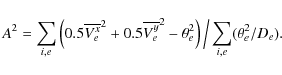
For a complete set of FORS2 observations (any seeing conditions), and images in the central r<1area, we obtained A=160 as. This value exceeds by much the standard deviation for epoch average residuals of bright stars, which is typically about 50-70 as, and therefore such systematic errors strongly affect the histogram's shape (Fig. 12b). It was found that large A values are associated with images of abnormally small FWHM, in particular FORS2 images in Dec 2006 with exceptionally good seeing of 0.3-0.5 . Elimination of images with seeing below 0.47 (3.7 px) and the subsequent rejection of bad images with (6.2 px) significantly improved A. Such filtration produced better solution with essentially more compact histograms of epoch-normalized residuals (Fig. 12c) fitted with a Gaussian of only 0.72 width parameter. This is insignificantly smaller than the expected -width which, due to a change in caused by the above filtering, decreased from 0.78 to 0.75. The described filtering of 20% of the FORS2 images, was applied to a few FORS1 images whose seeing was almost always within the limits adopted. At the end of this Section we discuss the probable relation between image size and systematic errors.

The frequency distribution of epoch average residuals based on merged residuals (Fig. 12d) does not differ from that built for V_e (Fig. 12c).

The estimates of A for stars in CCD central circular areas of r=40 , 1, and 1.5  are given in Table 4.

Table 4:   Systematic component A [as] in residuals V_e and in within central CCD zones of r radii.

According to Table 4, the characteristics of the systematic error Afor both cameras are similar and show a slight increase in the direction from the center to the periphery of a frame. Thus, while at the periphery A is near to 100 as, at r<40 it does not exceed 50-60 as. Due to statistical limitations we not can estimate A at the center (where the target is usually placed), but considering the tendency observed we predict it could be about 25 as at r<10 , as expected from the following discussion. The systematic components in and V_e are approximately equal.

An important piece of information on the global distribution of systematic errors over the CCD plane was derived applying a low-pass Gaussian spatial filter to the epoch residuals V_e. The resulting low-frequency component A(x,y) in V_e for each camera, some epochs, and reduction versions is shown in contour plots Figs. 13, 14 with isolines drawn with 25 as increments. All graphs refer to the residuals on the x-axis. A(x,y) function change is rather complicated and has several extremums. This behavior, of course, not can be approximated by polynomials with basic functions since this dependence is excluded in the course of the reduction procedure. It is characteristic that large systematic errors reaching in most cases 100-200 as tend to concentrate at the periphery. At the field center, where the target is usually placed, A(x,y) functions varies rather smoothly and often fall to <25 as. No graph was found to have extremum at the center of the frame.

In the case of FORS1, systematic error plots are given for middle 2002 epoch at which the maximum fluctuations of A(x,y) are detected. Figure 13a, plotted for V_e computed with k=10 at and Fig. 13b for merged residuals have few similar structures above 50 as. At the center, errors are negligibly small. Although we discuss here only a particular case of the reduction with k=10 or of merged , our comments (both for FORS1 and FORS2) are valid also for computations with other k due to the high correlation of results obtained at (Sect. 4.3).

Figure 14b shows the systematic pattern after elimination of images with abnormally good and bad seeing and illustrates the decrease of systematic errors compared to the use of a complete set of images (Fig. 14a). Few extrema have vanished and most contrast details are smoothed. These graphs correspond to the middle of the January 2007 epoch with the largest variance of monthly residuals (Fig. 11), which was chosen to show the worst case of A(x,y). In November 2006 (first epoch) these errors are much better (Fig. 14e). The error structure for the merged residuals (Fig. 14d) in general is like that for V_e (Fig. 14b) at the same epoch. Figure 14f refers to V_e computed at k=6 and . The distribution shown here is similar to that for the reduction with k=10 (Fig. 14b) and for with 50 as systematic errors at the center, but much larger peaks at frame boundaries.

The dependence of A(x,y) on x,y could be a reason for excluding systematic errors in a secondary iteration; however we had an insufficient number of reference stars. Alternatively, A_e can be treated as additional components of each star model parameter to be computed with other parameters. This however is not useful for planet search or microlensing applications due to the complete zeroing of useful astrometric signals.

Considering that a change of A_e between two adjacent epochs at the frame center is approximately 50 as (100-200 as within the entire FoV) for both cameras, we can estimate the stability of the FORS astrometric system over short time scales. Assuming that a given change occurs at about a month spacing, the daily rate of systematic change is 1-2 as (3-6 as for the whole FoV). Our previous study of FORS1 errors (Lazorenko et al. 2007) have shown that a difference in the systematic component over a time scale of four days is either undetectably small or 30 as atmost. This is about 8 as a day change in systematic errors in the whole FoV, which is in accord with the current estimate.

Recall that the amplitude of systematic errors of 50 as we referred to corresponds to poor observing conditions; the estimate of 25 as is more relevant for normal conditions and targets at frame center.

6.2 Instrumental background of systematic errors

Based on the discussion in the previous subsection, we conclude that the characteristics of the systematic component A_e in magnitude and in spatial behavior are identical for FORS1 and FORS2. This is the second identity of these cameras derived based on observations at rather different time scales, CCD type, and photometric bands (the first is a dependence of image motion variance on R), and is evidently due to identical optical design of the cameras.

Systematic errors are probably generated during image centroiding due to the highly complicated star profiles, actually indefinite at the high accuracies at which we work. Consider that a typical error of 100 as is only fraction of the FWHM. Although FORS images are appropriate, the definition of the ``image photocenter'' for star profiles distorted by variable optical aberrations becomes uncertain. Therefore we use a centroiding procedure (Lazorenko 2006) specialized for finding the weighted photocenter of the image which is more stable to image deformations than the ``profile center''.

At zero or constant geometric distortion, the position of the measured image centroid is subject only to random errors caused primarily by Poisson noise in the number of photons and by atmospheric image motion. Systematic and extra random components in position appear in the following cases of instability:

• small deformation of a star profile (change of asymmetry) in time due to a slow change of optical aberrations. This results in image photocenter shift proportional to the gradient of aberrations at the point. These shifts, correlated in x,y space, are detected (after a certain filtration introduced by astrometric reduction) as systematic residuals A(x,y); their change in time produces A component. The effect is lowest at frame center were images are most symmetric due to optimal optical performance;

• a random change of image-to-image atmospheric PSF and seeing (shape and size). This affects image profiles both in size and shape and therefore shifts photocenters by an amount proportional to seeing fluctuation and to the measure of image asymmetry at the point, representing modulation of the optical aberration field by a random signal. The observed effect is random in time and correlated in space, and thus mimics atmospheric image motion. In Sect. 5 we classified it as ``instrumental'' image motion with an amplitude exceeding that of atmospheric image motion and not dependent on exposure time.

The combined effect of image asymmetry and seeing variation is observed in an exaggerated form for stars with nearby companions, the light of which causes image asymmetry. It is easily detected as a linear dependence of V_im on FWHM, which in most bad seeing conditions produces enormous systematic deviations exceeding by much the random errors and being grounds for discarding these measurements (Sect. 2).

Systematic deviations of the average seeing at a single epoch from its average for a full set of data may produce systematic bias of positions. To see whether this exists in our data, we performed reduction with an expanded set of parameters adding two extra terms describing the linear dependence of a star's x,y position on seeing. With a full set (all seeing) of images, a new value of the systematic error A in an r<1 area decreased from its former 160 as to 90 as, and a much smoother shape of A(x,y) (Fig. 13c) was obtained in comparison to the initial pattern (Fig. 13a). The improvement, however, is seen primarily at the periphery where geometric distortions are largest. Thus variations of seeing actually lead to systematic errors in epoch positions. We however consider the use of the expanded reduction model insufficiently validated, since it reduces the useful astrometric signal and, for centrally placed targets, does not leads to a significant improvement in the accuracy.

Thus, variations in seeing are a source of systematic errors; for precise astrometry these variations should be limited.

7 Allan precision

Another characterization of the VLT long-term astrometric stability is based on the computation of the Allan deviation of residuals V_m. This quantity is normally used as a powerful indicator of systematic errors in observations and corresponds to the astrometric precision of a time series of n images. Figure 15 presents plots of this variable as a function of time lag (expressed as the number of images n) between subsamples of residuals V_m. The data in Fig. 15 are the average of each star Allan deviation taken over all, except the most peripheral, stars. Before averaging, we normalized the individual Allan deviations to their values at zero time lag so as to compensate for the highly varying amplitude of this variable for stars of different brightness. The right vertical axis of Fig. 15 is the scale for the normalized Allan deviation computed as described and is valid for stars of any magnitude. The left axis is the scale used to find the Allan deviation for bright stars (B=18 mag at FORS1 and R=16.5 mag at FORS2) with  as,  as and assuming its location at the frame center, which ensures small  as.

For computations, we used V_m residuals obtained with each reduction parameter k=6...16 and . Results for different k are very similar due to the high degree of correlation between these data sets (dashed curves in Fig. 15); for FORS2 they actually run into a single line corresponding to the Allan deviation of residuals . Besides, due to the normalizing procedure, computations based on a subset of either all or bright stars only produced similar estimates. The Allan deviation was found to follow (FORS1) and (FORS2) power laws which are near to that expected for the average of a random variable. A simple comparison with an n^-1/2 law is of course incorrect since least square fit residuals are correlated and have a non-diagonal covariance matrix . To compare our results with those expected with zero systematic errors, we performed a numerical simulation of observations introducing uncorrelated random noise in model measurements. The obtained dependence (solid curves in Fig. 15) follow a power law with a slope for both cameras, which is near to that obtained from observations.

The difference in the observed and expected plots is clearly seen for the FORS2 camera starting from n>15. This divergence is related to systematic errors discussed in Sect. 6. Due to the small magnitude of the errors, they cause only a 5-10% increase in the astrometric error in comparison to that expected in the absence of systematic errors.

Above, in the case of FORS2, we used images with a standard FWHM to avoid any degradation of precision caused by images with abnormal seeing. The Allan deviations with all available measurements used (black dots in Fig. 15) are seen to have an excess of about 30% for n>15.

Given a series of 30 images (0.5-1 h of telescope time), the precision of FORS1/2 astrometry (Fig. 15) is about 50 as. At this fixed number of images, Fig. 16 (open circles) shows the dependence of the precision on star brightness computed for each star as the individual Allan deviation. Data refer to FORS2 for which sufficiently long observation series are available and for images obtained at normal seeing. Because precision very much depends on the reference frame noise (especially for bright targets), the plot shows only those stars for which  as. For that reason, many of the brightest 16.5-17.0 mag stars were omitted due to their peripheral location in the frame. The observed dependence of precision on magnitude shows it to be better than 100 as for R<19 mag targets and about 50 as for  mag.

The above estimate includes the error caused by reference frame and optical aberrations which depend on a particular density of star distribution in the sky, stability of the optical system, and variations of seeing conditions at the period of observations. Precision improves with improved conditions. A case of interest is the precision expected at high reference star density ( ) and image motion  as, typical for a reference frame size of 0.7-1.5. These estimates, shown by a solid line in Fig. 16, prove the feasibility of 50 as astrometric precision for brightest targets.

8 Conclusion

Astrometric quantities (residuals of positions, model parameters) derived from the processing of images are intrinsically relative. They are computed in a certain system and relative to the frame of reference objects specific to the particular target. These peculiarities of differential reduction should be taken into account for the interpretation of the output data and in more complicated cases of handling inhomogeneous series of images, for instance obtained in different spectral bands or even with different cameras, which is a case expected for long-term programmes. We demonstrated that a careful processing of B and R images in a common system does not degrade precision.

The precision of astrometric imaging at VLT depends on several noise sources. Uncertainty of the image photocenter determination , of course, is the dominant component of the total error. Our data show that Eq. (1) provides a correct estimate of this error, at least with an accuracy of 5%, for a wide range of light fluxes and seeing conditions. depends not on the star magnitude but on the light flux collected in the star image. For that reason, the lowest (equally, best astrometric precision) is expected for images at saturation level, which depends on the exposure, filter, pixel scale, and seeing. Therefore, having, for example, dependence of on magnitude R, it is easy to apply it to other observations. For instance, in B band where is the difference of magnitudes of images with equal light flux in B and R bands. This scaling is illustrated in Fig. 9 where and are seen to be the same dependences shifted by  mag.

Mitigation of atmospheric image motion at  s exposure does not present a problem due to its small amplitude in comparison to other random noise components. Quite unexpectedly, however, we found that the measured image motion variance is the same at the very different T=70 and  s exposure. We consider this as a new type of random error caused by the combined effect of the telescope-related asymmetry of star profiles and of random changes in the atmospheric PSF. We have found that images with abnormally bad and good seeing are affected by large random and systematic errors and thus their use should be avoided in precision astrometry.

Estimates of astrometric errors obtained in this study refer rather to precision caused by stochastic error components but not to accuracy. The final astrometric accuracy can degrade compared to precision due to systematic errors incorporated into the reference frame and then propagated by the reduction model. Presently, our astrometric results cannot be cross-compared against independent datasets and analyses of common objects, which could provide direct estimates of the long-term accuracy. In Sect. 6,7, however, we demonstrated that the measured star displacements in space and time are fitted to nearly white noise residuals with a variance predicted by the model, therefore, an extra systematic component (if present) should closely trace both the parallactic and proper motion of each star. A too low probability of this scenario (considering large accumulated Dof) implies that the accuracy of the VLT relative parallax and proper motion determination is comparable to the precision.

We have demonstrated that, with reference to systematic errors, astrometry at FORS1/2 is accurate to 25 as at five month and 6 year time intervals. Due to that fact, relative proper motions and trigonometric parallaxes of stars in the test field were derived with a precision of 20 as yr^-1 and 40 as respectively for 17-19 mag stars. Thus distances to stars at 1 kpc can be measured with a precision of 4%, providing a correction from relative to absolute parallax is added. This level of accuracy and, especially, good long-term stability, has numerous astrometric applications including measurement of astrometric microlensing, planet detection and characterization by measuring reflex motion of the parent star, and kinematics of Galactic stellar populations. In the context of exoplanet searches, the use of the VLT to search for planets near brown dwarfs is very efficient. With a 2 year observation programm, Saturn mass planets with orbit periods longer than 1 year and Netpune mass planets with 2 year periods are detectable for brown dwarfs located at 10-20 pc. These observations will make a real breakthrough in our understanding of planet and brown dwarf formation by probing a separation and mass range that is poorly suited to other techniques.

Currently our method has several crucial limitations. It is applicable to moderately populated sky areas with low rates of blending but that are rich enough to provide a sufficient number of reference stars. Also, targets brighter than 15-16 mag not can be measured due to saturation if the exposure time is not too short. Therefore it is not applicable to highly crowded sky areas like those used for microlensing works and to bright, nearby solar-type stars which are objects of interest for planet searches. Most of these limitations originate from the star profile fitting and can be removed with use of a better technique for determination of star photocenters. Precision astrometry is also problematic for telescopes with segmented primary mirrors that produce intrinsic complex and time-variable PSF.

We emphasize that the results of this study do not refer to a specific telescope, they validate precision astrometry for a whole class of large ground-based imaging telescopes. Astrometry benefits highly from the use of large apertures, mitigating in this way both the principal image centroiding component of the total error and atmospheric image motion. For future 30 m telescopes, the astrometric precision is expected to be 10 as or better for image series of 0.5 h duration. At this precision, we are challenged with a wide spectrum of problems, e.g. the ability to measure bright objects due to saturation and the predominance of systematic errors caused by optical aberrations.

References

• Avila, G., Rupprecht, G., & Beckers, J. M. 1997, Proc. SPIE, 2871, 1135 [NASA ADS] (In the text)
• Boden, A. F., Colavita, M. M., Lane, B. F., et al. 1999, ASP Conf. Ser., 194, 84 [NASA ADS] (In the text)
• Cameron, P. B., Britton, M. C., & Kulkarni, S. R. 2008, AJ, 137, 83 [NASA ADS] [CrossRef] (In the text)
• Casertano, S., Lattanzi, M. G., Sozzetti, A., et al. 2008, A&A, 482, 699 [NASA ADS] [CrossRef] [EDP Sciences] (In the text)
• Delplancke, F., Leveque, S., Kervella, P., et al. 2000, Proc. SPIE 4006, 365 (In the text)
• Irwin, M. J. 1985, MNRAS, 214, 575 [NASA ADS] (In the text)
• Lane, B. F., & Muterspagh, M. W. 2004, ApJ, 601, 1129 [NASA ADS] [CrossRef] (In the text)
• Lane, B. F., Colavita, M. M., Boden, A. F., et al. 2000, Proc. SPIE, 4006, 452 [NASA ADS] (In the text)
• Lazorenko, P. F. 2002, A&A, 382, 1125 [NASA ADS] [CrossRef] [EDP Sciences] (In the text)
• Lazorenko, P. F. 2006, A&A, 449, 1271 [NASA ADS] [CrossRef] [EDP Sciences] (In the text)
• Lazorenko, P. F., & Lazorenko, G. A. 2004, A&A, 427, 1127 [NASA ADS] [CrossRef] [EDP Sciences] (In the text)
• Lazorenko, P. F., Mayor, M., Dominik, M., Pepe, F., et al. 2007, A&A, 471, 1057 [NASA ADS] [CrossRef] [EDP Sciences] (In the text)
• Lindegren, L. 1980, A&A, 89, 41 [NASA ADS] (In the text)
• Lindegren, L., Babusiaux, C., Bailer-Jones, C., et al. 2007, in A Giant Step: from Milli- to Micro-arcsecond Astrometry, ed. W. J. Jin, I. Platais, & M. A. C. Perryman, Proc. IAU Symp., 248, 217 (In the text)
• Monet, D. G., Dahn, C. C., Vrba, F. J., et al. 1992, AJ, 103, 638 [NASA ADS] [CrossRef] (In the text)
• Motch, C., Zavlin, V. E., & Haberl, F. 2003, A&A, 408, 323 [NASA ADS] [CrossRef] [EDP Sciences] (In the text)
• Moutou, C., Pont, F., Bouchy, F., & Mayor, M. 2004, A&A, 424, L31 [NASA ADS] [CrossRef] [EDP Sciences] (In the text)
• Muterspagh, M. W., Lane, B. F., Konacki, M., et al. 2006, Proc. SPIE, 6268, 16 (In the text)
• Perryman, M. A. C., de Boer, K. S., Gilmore, G., et al. 2001, A&A, 369, 339 [NASA ADS] [CrossRef] [EDP Sciences] (In the text)
• Pravdo, S., & Shaklan, S. 1996, AJ, 465, 264 [NASA ADS] [CrossRef] (In the text)
• Shao, M., & Colavita, M. M. 1992, A&A, 262, 353 [NASA ADS] (In the text)

Footnotes

... FORS1/2

Based on observations made with ESO telescopes at the La Silla Paranal Observatory under programme ID 078.C-0074 and observations made with the European Southern Observatory telescopes obtained from the ESO/ST-ECF Science Archive Facility.

...

Royal Society University Research Fellow.

All Tables

Table 1:   Summary of the test field observations.

Table 2:   Minimum and optimal radii of reference fields.

Table 3:   Coefficients of Eq. (34): derived in this study B[as], b; predicted , by atmospheric model (Lazorenko & Lazorenko 2004); and B', b' obtained from a single series of FORS2 images (Lazorenko 2006).

Table 4:   Systematic component A [as] in residuals V_e and in within central CCD zones of r radii.

All Figures

---

Copyright ESO 2009