| Issue |
A&A
Volume 504, Number 3, September IV 2009
|
|
|---|---|---|
| Page(s) | 705 - 717 | |
| Section | Cosmology (including clusters of galaxies) | |
| DOI | https://doi.org/10.1051/0004-6361/200912424 | |
| Published online | 16 July 2009 | |
Constrained correlation functions
P. Schneider - J. Hartlap
Argelander-Institut für Astronomie, Universität Bonn, Auf dem Hügel 71, 53121 Bonn, Germany
Received 5 May 2009 / Accepted 7 July 2009
Abstract
Measurements of correlation functions and their comparison with theoretical models are often employed in natural sciences, including astrophysics and cosmology, to determine best-fitting
model parameters and their confidence regions. Due to a lack of better descriptions, the likelihood function of the correlation function is often assumed to be a multi-variate Gaussian. Using different methods, we show that correlation functions have to satisfy constraint relations, owing to the non-negativity of the power spectrum of the underlying random process. Specifically, for any statistically homogeneous and (for more than one spatial dimension) isotropic random field with
correlation function ![]() ,
we derive inequalities for the correlation coefficients
,
we derive inequalities for the correlation coefficients
![]() (for integer n) of the form
(for integer n) of the form
![]() ,
where the
lower and upper bounds on rn depend on the rj, with j<n, or more explicitly
,
where the
lower and upper bounds on rn depend on the rj, with j<n, or more explicitly
![]() Explicit expressions for the bounds are obtained for arbitrary n. We show that these constraint equations very significantly limit the set of possible correlation functions. For one particular example of a fiducial cosmic shear survey, we show that the Gaussian likelihood ellipsoid has a
significant spill-over into the region of correlation functions forbidden by the aforementioned constraints, rendering the resulting best-fitting model parameters and their error region questionable, and indicating the need for a better description of the likelihood function. We conduct some simple numerical experiments which explicitly demonstrate the failure of a Gaussian description for the likelihood of
Explicit expressions for the bounds are obtained for arbitrary n. We show that these constraint equations very significantly limit the set of possible correlation functions. For one particular example of a fiducial cosmic shear survey, we show that the Gaussian likelihood ellipsoid has a
significant spill-over into the region of correlation functions forbidden by the aforementioned constraints, rendering the resulting best-fitting model parameters and their error region questionable, and indicating the need for a better description of the likelihood function. We conduct some simple numerical experiments which explicitly demonstrate the failure of a Gaussian description for the likelihood of ![]() .
Instead, the shape of the likelihood function of the correlation coefficients appears to follow approximately the shape of the bounds on the rn, even
if the Gaussian ellipsoid lies well within the allowed region. Therefore, we define a non-linear and coupled transformation of the rn, based on these bounds. Some numerical experiments then
indicate that a Gaussian is a much better description of the likelihood in these transformed variables than of the original correlation coefficients - in particular, the full probability
distribution then lies explicitly in the allowed region. For more than one spatial dimension of the random field, the explicit expressions of the bounds on the rn are not optimal. We outline a
geometrical method how tighter bounds may be obtained in principle. We illustrate this method for a few simple cases; a more general treatment awaits future work.
.
Instead, the shape of the likelihood function of the correlation coefficients appears to follow approximately the shape of the bounds on the rn, even
if the Gaussian ellipsoid lies well within the allowed region. Therefore, we define a non-linear and coupled transformation of the rn, based on these bounds. Some numerical experiments then
indicate that a Gaussian is a much better description of the likelihood in these transformed variables than of the original correlation coefficients - in particular, the full probability
distribution then lies explicitly in the allowed region. For more than one spatial dimension of the random field, the explicit expressions of the bounds on the rn are not optimal. We outline a
geometrical method how tighter bounds may be obtained in principle. We illustrate this method for a few simple cases; a more general treatment awaits future work.
Key words: methods: statistical - cosmological parameters - cosmology: miscellaneous
1 Introduction
One of the standard ways to obtain constraints on model parameters of a stochastic process is the determination of its two-point correlation function
![]() from observational data, where
from observational data, where
![]() is the separation vector between pairs of points. This observed correlation function is then compared with the corresponding correlation function
is the separation vector between pairs of points. This observed correlation function is then compared with the corresponding correlation function
![]() from a model, where p denotes the model parameter(s). A commonly used method for this comparison is the consideration of the likelihood function
from a model, where p denotes the model parameter(s). A commonly used method for this comparison is the consideration of the likelihood function
![]() ,
which yields the probability for observing the correlation
function
,
which yields the probability for observing the correlation
function
![]() for a given set of parameters p. It is common (see Seljak & Bertschinger 1993, for an application to microwave background anisotropies; Fu et al. 2008, for a cosmic shear analysis; or Okumura et al. 2008, for an application to the spatial correlation function of galaxies) to approximate this likelihood by a Gaussian,
for a given set of parameters p. It is common (see Seljak & Bertschinger 1993, for an application to microwave background anisotropies; Fu et al. 2008, for a cosmic shear analysis; or Okumura et al. 2008, for an application to the spatial correlation function of galaxies) to approximate this likelihood by a Gaussian,
![$\displaystyle %
{\cal L}(\{\xi(x_i)\}\vert p)
\propto \exp\left[ - {1\over 2} \...
...p) \right]~{\rm\tens{Cov}}^{-1}_{ij}\left[ \xi(x_j)-\xi(x_j;p) \right] \right],$](/articles/aa/full_html/2009/36/aa12424-09/img40.png)
where it has been assumed that the random field is homogeneous and isotropic, so that the correlation function depends only on the absolute value of the separation vector. Furthermore, it has been assumed that the correlation function is obtained at discrete points xi; for an actual measurement, one usually has to bin the separation of pairs of points, in which case xi is the central value of the bin. In (1),
In Hartlap et al. (2009) we have investigated the likelihood function for the cosmic shear correlation function and found that it deviates significantly from a Gaussian. This study relied on numerical ray-tracing simulations through the density field obtained from N-body simulations of the large-scale structure in the Universe.
In this paper, we will show that the likelihood function of the correlation function cannot be a Gaussian. In particular, we show that any correlation function obeys strict constraints, which can be expressed as
for arbitrary x and integer n; these constraints can be derived by several different methods. With one of these methods, one can derive explicit equations for the upper and lower bounds in (2) for arbitrary values of n. The basic reason for the occurrence of such constraints is the non-negativity of the power spectrum, or equivalently, the fact that covariance matrices of the values of a random fields at different positions are positive (semi-)definite. For
The outline of the paper is as follows: in Sect. 2, we obtain bounds on the correlation function using the Cauchy-Schwarz inequality, as well as making use of the positive definiteness of the covariance matrix of random fields. It turns out that the latter method gives tighter constraints on ![]() ;
in fact, these constraints are optimal for one-dimensional random fields. We show in Sect. 3 that these bounds significantly constrain the set of functions which can possibly be correlation functions. Whereas the bounds obtained in Sect. 2 are valid for any dimension of the random field, they are not optimal in more than one dimension; we consider generalizations to higher-order random fields, and to arbitrary combinations of separations xi in Sect. 4. In Sect. 5 we introduce a non-linear coupled transformation of the correlation coefficients based on the bounds; for the case of a one-dimensional field, all combinations of values in these transformed quantities correspond to allowed correlation functions (meaning that one can find a non-negative power spectrum yielding the corresponding correlations). Hence, a Gaussian probability distribution of these transformed variables appears to be more realistic than one for the correlation function itself. This expectation is verified with some
numerical experiments which are described in Sect. 6. Furthermore, we show that for a fiducial cosmological survey the Gaussian likelihood for the correlation function can significantly overlap with the region forbidden by (2), depending on survey size and number of
separations at which the correlation function is measured. We conclude with a discussion and an outlook to future work and open questions.
;
in fact, these constraints are optimal for one-dimensional random fields. We show in Sect. 3 that these bounds significantly constrain the set of functions which can possibly be correlation functions. Whereas the bounds obtained in Sect. 2 are valid for any dimension of the random field, they are not optimal in more than one dimension; we consider generalizations to higher-order random fields, and to arbitrary combinations of separations xi in Sect. 4. In Sect. 5 we introduce a non-linear coupled transformation of the correlation coefficients based on the bounds; for the case of a one-dimensional field, all combinations of values in these transformed quantities correspond to allowed correlation functions (meaning that one can find a non-negative power spectrum yielding the corresponding correlations). Hence, a Gaussian probability distribution of these transformed variables appears to be more realistic than one for the correlation function itself. This expectation is verified with some
numerical experiments which are described in Sect. 6. Furthermore, we show that for a fiducial cosmological survey the Gaussian likelihood for the correlation function can significantly overlap with the region forbidden by (2), depending on survey size and number of
separations at which the correlation function is measured. We conclude with a discussion and an outlook to future work and open questions.
2 Upper and lower bounds on correlation functions
Consider an n-dimensional homogeneous and isotropic random field
![]() ,
with vanishing expectation value
,
with vanishing expectation value
![]() ,
and with power spectrum
,
and with power spectrum
![]() and correlation function
and correlation function

which depends only on the absolute value of
owing to

where J0 is the Bessel function of the first kind of zero order. Since J0(x) has an absolute minimum at

where
In the following, we will concentrate mainly on the one-dimensional case and write

However, higher dimensions of the random field are included in all what follows, since by specifying
which thus takes the same form as (7). Thus, the n-dimensional case can be included in the same formalism as the one-dimensional case; note that for this argument, the random field is not restricted to be isotropic. However, as we shall discuss later, the resulting inequalities will not be optimal for isotropic fields of higher dimension.
In the foregoing equations, P(k) can correspond either to the power spectrum of the underlying random process, or the sum of the underlying process and statistical noise. Furthermore, the power spectrum can also be the square of the Fourier transform of the realization of a random process in a finite sample volume. In all these cases, the non-negativity of P(k) applies, and the constraints on the corresponding correlation function derived below must hold.
2.1 Constraints from the Cauchy-Schwarz inequality
Making use of the Cauchy-Schwarz inequality,
![\begin{displaymath}%
\left[ \int_0^\infty {\rm d}k\; f(k)~h(k) \right]^2
\le \int_0^\infty {\rm d}k\; f^2(k)\;\int_0^\infty {\rm d}k\; h^2(k),
\end{displaymath}](/articles/aa/full_html/2009/36/aa12424-09/img66.png) |
(9) |
we obtain by setting
| (10) |
where we made use of the identity

The interpretation of this constraint can be better seen in terms of the correlation coefficient

This result can be interpreted as follows: if two points separated by x are strongly correlated,
Making use of the identity
![\begin{eqnarray*}\left[ \cos a+\cos(2a) \right]^2=\left[ 1+\cos a \right]~\left[ 1+\cos (3a) \right],
\end{eqnarray*}](/articles/aa/full_html/2009/36/aa12424-09/img75.png)
and applying the Cauchy-Schwarz inequality with
![\begin{displaymath}%
\left[ \xi(x)+\xi(2 x) \right]^2\le \left[ \xi(0)+\xi(x) \right]~\left[ \xi(0)+\xi(3 x) \right].
\end{displaymath}](/articles/aa/full_html/2009/36/aa12424-09/img78.png) |
(13) |
A second inequality is obtained by using in a similar way the identity
![\begin{eqnarray*}\left[ \cos a-\cos(2a) \right]^2=\left[ 1-\cos a \right]~\left[ 1-\cos (3a) \right].
\end{eqnarray*}](/articles/aa/full_html/2009/36/aa12424-09/img79.png)
Both of these inequalities are summarized in terms of the correlation coefficient as

Further inequalities involving
![\begin{eqnarray*}&& [\cos a+\cos(n-1)a]^2=[1+\cos(n a)]~[1+\cos(n-2)a];\\
&& [\cos a-\cos(n-1)a]^2=[1-\cos(n a)]~[1-\cos(n-2)a]
\end{eqnarray*}](/articles/aa/full_html/2009/36/aa12424-09/img83.png)
for

where the special case n=3 has been derived already. We have thus found a set of inequalities for all correlation coefficients rn. In the next section, we will obtain bounds on the correlation function using a different method, and will show that these ones are stricter than those in (15).
2.2 Constraints from a covariance matrix approach
We will proceed in a different way which is more straightforward. Consider a set of N points
xm= m x, with m integer and
![]() .
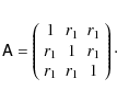
The covariance matrix of the random field at these N points has the simple form
.
The covariance matrix of the random field at these N points has the simple form
 |
(16) |
As is well known, the covariance matrix must be positive semi-definite, i.e., its eigenvalues must be non-negative. Dividing

and the eigenvalues of
| (18) |
i.e. we reobtain (4). For N=3, the eigenvalues read
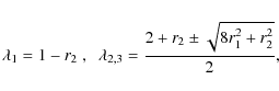
and the conditions
![\begin{eqnarray*}\lambda_{1,2,3,4}=1 \pm {1\over 2}\left[ r_1+r_3
\pm\sqrt{5 r_1^2-8 r_1 r_2+4 r_2^2-2 r_1 r_3+r_3^2} \right],
\end{eqnarray*}](/articles/aa/full_html/2009/36/aa12424-09/img97.png)
and the conditions
However, we do not need an explicit expression for the eigenvalues, but only need to assure that they are non-negative. This condition can be formulated in a different way. The eigenvalues of the matrix ![]() are given by the roots of the characteristic polynomial, which is the determinant of the matrix
are given by the roots of the characteristic polynomial, which is the determinant of the matrix
![]() .
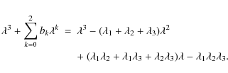
For a given N, this polynomial is of order N in
.
For a given N, this polynomial is of order N in ![]() and of the form
and of the form

The coefficients bk of the polynomial are functions of the rk, as obtained from calculating the determinant. On the other hand, they can be expressed by the roots
The condition that all
This procedure can be generalized for arbitrary N: the condition that all eigenvalues of the correlation matrix ![]() are non-negative is equivalent to requiring that the coefficients of the characteristic polynomial (19) satisfy
are non-negative is equivalent to requiring that the coefficients of the characteristic polynomial (19) satisfy
![]() if n is odd, and
if n is odd, and
![]() if n is even. The explicit calculation of the characteristic polynomial by hand becomes infeasible, hence we use the computer algebra program Mathematica (Wolfram 1996). For successively larger N, we calculate the characteristic polynomial. As we will show below, the
characteristic polynomial factorizes into two polynomials; if N is even, it factorizes into two polynomials of order N/2, whereas if N is odd, it factorizes into polynomials of order
if n is even. The explicit calculation of the characteristic polynomial by hand becomes infeasible, hence we use the computer algebra program Mathematica (Wolfram 1996). For successively larger N, we calculate the characteristic polynomial. As we will show below, the
characteristic polynomial factorizes into two polynomials; if N is even, it factorizes into two polynomials of order N/2, whereas if N is odd, it factorizes into polynomials of order
![]() .
The condition that all eigenvalues are non-negative is equivalent to the condition that the roots of both polynomials are non-negative; this condition can be translated into inequalities for the coefficients of the polynomials in the same way as described above.
.
The condition that all eigenvalues are non-negative is equivalent to the condition that the roots of both polynomials are non-negative; this condition can be translated into inequalities for the coefficients of the polynomials in the same way as described above.
We illustrate this procedure for the case N=5. The characteristic polynomial in this case becomes
 |
(20) |
with
| b1 | = | r2+r4-2, | |
| b0 | = | (1-r2)(1-r4)-(r1-r3)2, | |
| c2 | = | -3-r2-r4, | |
| c1 | = | 3(1-r12)-2r1 r3-r32+2r4+r2(2+r4)-2 r22, | |
| c0 | = | (2 r12-1-r2)r4+r32+2 r1 r3(1-2r22) | |
| + 2r22(1+r2) -r2+r12(3-4r2)-1. |
The conditions

Alternatively, one can use the function InequalitySolve of Mathematica for the five inequalities for the four coefficients, to obtain the same result.
We see that the upper bound in (21) agrees with that obtained from the Cauchy-Schwarz inequality - see (15) - but the lower bounds differ. Hence, for n=4 the bounds on rn derived from the two methods are different, and that will be the case for all ![]() .
This is not surprising, since the Cauchy-Schwarz inequality does not make any statement on
how ``sharp'' the bounds are, i.e., whether the bounds can actually be approached. One can argue, using discrete Fourier transforms, that the bounds obtained from the covariance method are ``sharp'' (for a one-dimensional field) in the sense that for each combination of allowed rn, one can find a non-negative power spectrum corresponding to these correlation coefficients - the bounds can
therefore not be narrowed further.
.
This is not surprising, since the Cauchy-Schwarz inequality does not make any statement on
how ``sharp'' the bounds are, i.e., whether the bounds can actually be approached. One can argue, using discrete Fourier transforms, that the bounds obtained from the covariance method are ``sharp'' (for a one-dimensional field) in the sense that for each combination of allowed rn, one can find a non-negative power spectrum corresponding to these correlation coefficients - the bounds can
therefore not be narrowed further.
It should be noted that in the cases given above, the lower (upper) bound on rn is a quadratic function in rn-1, and its quadratic term
c rn-12 has a positive (negative) coefficient c. This implies that the allowed region in the
rn-1-rn-plane is convex; indeed, as we will show below, the allowed n-dimensional region for the
![]() is convex.
is convex.
The procedure illustrated for the case N=5 holds for larger N as well: only the coefficients of ![]() in the two polynomials yield new constraints on the correlation coefficient rN-1, and these two coefficients are linear in rN-1, so the constraints for
rN-1 can be obtained explicitly. This then leads us to conclude that the positive-definiteness of the matrix
in the two polynomials yield new constraints on the correlation coefficient rN-1, and these two coefficients are linear in rN-1, so the constraints for
rN-1 can be obtained explicitly. This then leads us to conclude that the positive-definiteness of the matrix ![]() for a given N is equivalent to the positivity of the determinants of all
submatrices which are obtained by considering only the first n rows and columns of
for a given N is equivalent to the positivity of the determinants of all
submatrices which are obtained by considering only the first n rows and columns of ![]() ,
with
,
with
![]() .
We will make use of this property in the next subsection.
.
We will make use of this property in the next subsection.
For larger N, the upper and lower bounds are given by quite complicated expressions, so we refrain from writing them down; however, using the output from Mathematica, they can be used for subsequent numerical calculations. A much more convenient method for calculating the upper and lower bounds explicitly will be obtained below.
To summarize, the procedure outlined gives us constraints on the form
| (22) |
where the lower and upper bounds are function of the rk, k<n, and satisfy
The existence of these upper and lower bounds on rn, and thus on the correlation function, immediately implies that the likelihood function of the correlation function cannot be a Gaussian, since the support of the latter is unbounded. This does not imply necessarily that the Gaussian approximation is bad; if the Gaussian probability ellipsoid described by (1) is ``small'' in the sense that it is well contained inside the allowed region, the existence of the bounds alone yields no estimate for the accuracy of the Gaussian approximation. We will come back to this issue in Sect. 6.
Whereas the expressions for
![]() and
and
![]() for larger n become quite long, we found a remarkable result for the difference
for larger n become quite long, we found a remarkable result for the difference
![]() .
This is most easily expressed by defining the functions
.
This is most easily expressed by defining the functions
| (23) |
Then, for odd n

and for even n,

This result has been obtained by guessing, and subsequently verified with Mathematica, up to n=16, using the explicit expressions for the bounds derived next. We will make use of these properties in the Sect. 3.
2.3 Explicit expression for the bounds
We will now derive an explicit expression for the upper and lower bounds on the rn. In doing so, we will first show that the determinant of the matrix ![]() for N points factorizes into two
polynomials, both of which are linear in rN-1. Then we make use of the fact that the positive definiteness of
for N points factorizes into two
polynomials, both of which are linear in rN-1. Then we make use of the fact that the positive definiteness of ![]() is equivalent to having positive determinant of all submatrices obtained from
is equivalent to having positive determinant of all submatrices obtained from ![]() by considering only the first n rows and columns,
by considering only the first n rows and columns, ![]() ;
however, these submatrices of
;
however, these submatrices of ![]() correspond to the matrix
correspond to the matrix ![]() for lower numbers of points, and their positive determinant is equivalent to the upper and lower bounds on the rn for
for lower numbers of points, and their positive determinant is equivalent to the upper and lower bounds on the rn for ![]() .
Hence, by increasing N successively, the constraints on rN-1 are obtained from requiring
.
Hence, by increasing N successively, the constraints on rN-1 are obtained from requiring
![]() .
.
The determinant of a matrix is unchanged if a multiple of one row (column) is added to another row (column). We make use of this fact for the calculation of
![]() ,
by carrying out the following four steps:
,
by carrying out the following four steps:
- 1.
- We add the first row to the last, obtaining the matrix
 with
elements
with
elements

- 2.
- We subtract the last column from the first,

- 3.
- The second row is added to the (N-1)-st one, the third row is added to the (N-2)-nd one, and so on. For N odd, this reads

whereas for N even, the sum extends to (N-2)/2. - 4.
- Finally, the (N-1)-st column is subtracted from the second one, the (N-2)-nd column is subtracted from the third one, and so on, which for odd N reads

whereas for even N the sum extends to (N-2)/2.
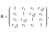
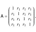
 |
Figure 1:
For N=7, the original covariance matrix |
| Open with DEXTER | |
These steps are illustrated for the case N=7 in Fig. 1. For N even [odd], this results in a matrix
![]() which contains in the lower left corner a N/2
which contains in the lower left corner a N/2 ![]() N/2 ((N-1)/2
N/2 ((N-1)/2 ![]() (N+1)/2) submatrix with elements zero. Therefore, the determinant of
(N+1)/2) submatrix with elements zero. Therefore, the determinant of
![]() factorizes into the determinants of two N/2
factorizes into the determinants of two N/2 ![]() N/2 matrices (of a (N-1)/2
N/2 matrices (of a (N-1)/2 ![]() (N-1)/2 and of a (N+1)/2
(N-1)/2 and of a (N+1)/2 ![]() (N+1)/2 matrix). Thus,
(N+1)/2 matrix). Thus,
 |
(26) |
where we explicitly indicate the number N of points, and thus the dimensionality of
 |
(27) |
whereas for odd N,
| (28) |
Since

where
 |
(30) |
where we set n=N-1. Analogously, the final element of
 |
(31) |
where
 |
(32) |
Since
 |
(33) |
The analogous result holds for the
 |
(34) |
These recursion relations then yield the explicit expressions
 |
|||
 |
(35) |
for N even, and
 |
|||
 |
(36) |
for N odd. This yields for the determinant of the matrix
 |
(37) |
for even and odd N, respectively. Accordingly, the width
 |
(38) |
where we made use of (24) and (25).
3 How strong are the constraints?
We shall now investigate the question how constraining the constraints on the correlation function or, equivalently, the correlation coefficients are. In order to quantify this question, we imagine that the correlation function is measured on a regular grid of separations n x, and from that we define as before
![]() .
Due to (4),
.
Due to (4),
![]() for all n. We therefore consider the set of functions defined by their values on the grid points, and allow only
values in the interval
for all n. We therefore consider the set of functions defined by their values on the grid points, and allow only
values in the interval
![]() for all n. Let M be the largest value of n that we consider; then the functions we consider are defined by a point in the M-dimensional space spanned by the rn. This M-dimensional cube has sidelength 2 and thus a volume of 2M. We will now investigate which fraction of this volume corresponds to correlation functions which satisfy the constraints derived in the previous section.
for all n. Let M be the largest value of n that we consider; then the functions we consider are defined by a point in the M-dimensional space spanned by the rn. This M-dimensional cube has sidelength 2 and thus a volume of 2M. We will now investigate which fraction of this volume corresponds to correlation functions which satisfy the constraints derived in the previous section.
A related question that can be answered is: suppose the values of rk,
![]() are given; what fraction of the (M-n)-dimensional subspace, spanned by the rk with
are given; what fraction of the (M-n)-dimensional subspace, spanned by the rk with
![]() corresponds to allowed correlation functions? For example, if r1=1, then all other rk=1, and hence the condition r1=1 is very constraining - the volume fraction of the subspace spanned by the rk with
corresponds to allowed correlation functions? For example, if r1=1, then all other rk=1, and hence the condition r1=1 is very constraining - the volume fraction of the subspace spanned by the rk with ![]() is zero in this case.
is zero in this case.
Mathematically, we define these volume fractions as
| VMn | = |  |
|
| = |  |
(39) |
The factor 1/2 in each integration accounts for the side-length of the (M-n)-dimensional cube, so that the VMn are indeed fractional volumes. VMn depends on the rk with
 |
(40) |
We can therefore calculate the VMn iteratively, starting with
 |
(41) |
where we have skipped the integration limits; here and in the following, an integral over rn always extends from
It should be noted that the only dependence of
VM(M-1) on rM-1 is through the factor
![]() .
Therefore, the next recursion step reads
.
Therefore, the next recursion step reads
| VM(M-2) | = | ||
| = |  |
||
| = |  |
||
| = |  |
(42) |
where

For the next step we notice that the only dependence of VM(M-2) on rM-2 is through the function
| VM(M-3) | = | ||
| = |  |
||
| = |  |
(44) |
where we made again use of (43). Based on these results, we can now obtain a general expression,
 |
(45) |
which can be proved by induction. In particular, the
![\begin{displaymath}%
V_M=2^{M(M-1)}\left[ \prod_{k=2}^M {\rm B}(k,k) \right].
\end{displaymath}](/articles/aa/full_html/2009/36/aa12424-09/img201.png)
The values of VM up to M=20 are shown in Fig. 2. As can be seen from the upper panel, the admissible volume very quickly decreases as M increases. For comparison, in the lower panel we show VM1/M, i.e. the typical diameter of the allowed region.
![\begin{figure}
\par\includegraphics[width=8.8cm,clip]{figs/volfrac.eps}
\end{figure}](/articles/aa/full_html/2009/36/aa12424-09/img202.png) |
Figure 2: Upper panel: volume fraction VM (Eq. (46)) as function of the number M of separations for which the correlation function is measured. Lower panel: VM1/M as function of M. One sees that the typical linear dimension of the allowed region decreases with M, meaning that the strong decrease of VM with M is not just an effect of the dimensionality of the volume considered. |
| Open with DEXTER | |
4 Generalizations
The considerations of the previous sections were restricted to correlation functions as measured at equidistant points xn=n x. In some cases, however, it may be advantageous to drop this constraint, e.g., to consider the correlation function at logarithmically spaced points. Furthermore, as mentioned before, tighter constraints on the correlation function are expected to hold in the multi-dimensional case. We shall consider these aspects in this section, presenting another method for deriving constraints which yields the optimal constraints for arbitrarily spaced points xn in one- or higher-dimensional fields. But before, we briefly consider the covariance method for higher dimensions.
4.1 Higher-dimensional fields: the covariance method
As was noted above, the inequalities for the correlation functions have been obtained with a one-dimensional random field in mind. Whereas we have shown that all the bounds on correlation
functions are also valid for higher-dimensional fields, they are not assumed to be ``optimal'' - the reason is that the equivalent one-dimensional power spectrum defined in (7) was
assumed to be totally arbitrary, except from being non-negative, whereas for isotropic fields in higher dimensions, it will obey further constraint relations due to the (n-1)-dimensional
integration in (8). A first indication that the bounds can be improved has been seen with the lower bounds on the ratio
![]() ,
which turned out to be larger for two and three
dimensions than for a one-dimensional field. The foregoing constraints on the correlation function are re-obtained with the covariance matrix approach in higher dimensions if the set of points
are placed equidistant along one direction. New (and stronger) constraints are expected from this method if the distribution of points makes use of these higher dimensions.
,
which turned out to be larger for two and three
dimensions than for a one-dimensional field. The foregoing constraints on the correlation function are re-obtained with the covariance matrix approach in higher dimensions if the set of points
are placed equidistant along one direction. New (and stronger) constraints are expected from this method if the distribution of points makes use of these higher dimensions.
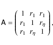
As a first example, we consider a two-dimensional (or higher-dimensional) field and place three points in an equilateral triangle of side-length x. The separation between any pair of points
is then x, and the covariance matrix of these three points, normalized by ![]() ,
then reads
,
then reads
The eigenvalues of this matrix are
for all x. The lower bound is somewhat smaller than the one obtained earlier for two-dimensional random fields,
and its eigenvalues are

where we also used (47).
Finally, we consider a square of side-length x, for which the covariance matrix reads
with the eigenvalues
 |
(49) |
which is a weaker constraint than (48) for
Finally, we consider the simplest case in three dimensions, namely a set a of four points arranged in a regular tetrahedron of sidelength x. The resulting covariance matrix is
with eigenvalues
| (50) |
a constraint stronger than the ones obtained for one and two dimensions, but falling short of the one derived from the global minimum of the spherical Bessel function,
![\begin{figure}
\par\includegraphics[width=17cm,clip]{figs/fig3.eps}
\end{figure}](/articles/aa/full_html/2009/36/aa12424-09/img245.png) |
Figure 3:
Left panel: the curve
|
| Open with DEXTER | |
4.2 Optimal constraints in the general case
We now describe a general method for deriving constraints on correlation functions ![]() of homogeneous and isotropic random fields, allowing for arbitrary values of separations xn and
arbitrary dimensions. However, it should be said right at the beginning that we were unable to obtain the corresponding bounds on the correlation functions explicitly.
of homogeneous and isotropic random fields, allowing for arbitrary values of separations xn and
arbitrary dimensions. However, it should be said right at the beginning that we were unable to obtain the corresponding bounds on the correlation functions explicitly.
We can write the general relation (3) in the form
 |
(51) |
where
 |
(52) |
where the wj are (positive) weights corresponding to the quadrature formula, and in the last step we defined
 |
(53) |
where the coefficients
![\begin{displaymath}%
V_i=\left[ \sum_{j=1}^K W_j \right]^{-1} W_i
\end{displaymath}](/articles/aa/full_html/2009/36/aa12424-09/img257.png) |
(54) |
satisfy
If we now consider a set of N points xn, together with the correlation coefficients
![]() ,
then we see that a point in the N-dimensional space of
,
then we see that a point in the N-dimensional space of
![]() can be
described as a weighted sum of points lying along the curve
can be
described as a weighted sum of points lying along the curve
![]() ,
,
![]() ,
i.e.,
,
i.e.,
 |
(55) |
where we considered the transition of the discrete points kj to a continuous variable
Unfortunately, we have not found a way how to algebraically describe the convex envelope of the curve
![]() ,
and thus to obtain explicit expressions for the upper and lower bounds on ri. For now, we therefore will present just a few simple examples.
,
and thus to obtain explicit expressions for the upper and lower bounds on ri. For now, we therefore will present just a few simple examples.
For the 1-dimensional case with two points
x2= 2 x1, the curve reads
![]() ,
with
,
with
![]() ;
the same set of points is described by the
curve
;
the same set of points is described by the
curve
![]() (using trigonometric identities),
(using trigonometric identities),
![]() .
Thus, the convex envelope of
.
Thus, the convex envelope of ![]() is the region between the parabola
is the region between the parabola ![]() and the line r2=+1, and thus we re-obtain the bounds (11). For the choice x2 = 3 x1, the set of points of
and the line r2=+1, and thus we re-obtain the bounds (11). For the choice x2 = 3 x1, the set of points of
![]() is equivalent to that of the curve
is equivalent to that of the curve
![]() ,
,
![]() .
The convex envelope can then be described by the bounds
.
The convex envelope can then be described by the bounds
![]() ,
where the lower bound differs from -1 for r1> 1/2, and the upper bound is different from +1 for r1< -1/2. If we choose instead
,
where the lower bound differs from -1 for r1> 1/2, and the upper bound is different from +1 for r1< -1/2. If we choose instead
![]() ,
then for a generic (non-rational)
,
then for a generic (non-rational) ![]() ,
the curve
,
the curve
![]() fills the whole square
fills the whole square
![]() ,
,
![]() ,
which is also coincident with its convex envelope.
,
which is also coincident with its convex envelope.
As the next example, we consider a 2-dimensional field with x2=2 x1. In the left panel of Fig. 3, the curve
![]() is plotted for
is plotted for
![]() .
The convex envelope in this case can be constructed explicitly: the boundary of the smallest convex region which contains the curve
.
The convex envelope in this case can be constructed explicitly: the boundary of the smallest convex region which contains the curve ![]() is composed of four parts: (1) the section of the curve
is composed of four parts: (1) the section of the curve
![]() for
for
![]() ;
(2) the straight line
connecting the two points
;
(2) the straight line
connecting the two points
![]() and
and
![]() ;
(3) the section of the curve
;
(3) the section of the curve
![]() for
for
![]() ;
and (4) the straight line connecting
;
and (4) the straight line connecting
![]() and
and
![]() .
In a similar way, the convex envelope can be constructed for a 3-dimensional random field; see Fig. 3, middle panel.
.
In a similar way, the convex envelope can be constructed for a 3-dimensional random field; see Fig. 3, middle panel.
Unfortunately, we have not yet found a systematic way how to construct the convex envelope for n>2, and how to obtain explicit bounds on the correlation coefficients in these cases - although it is clear that the allowed region, at least in the r1-r2-plane, decreases as one goes to higher-dimensional fields (see right panel of Fig. 3). Therefore, the development of explicit bounds in higher dimensions is of great interest.
5 Transformation of variables
The finite bounds on the correlation coefficients clearly show that the likelihood of the correlation function cannot be a Gaussian. However, the bounds on rn may suggest that the Gaussian approximation for the likelihood could be better in terms of transformed variables, in which the allowed range for each rn is mapped onto the real axis. Such a transformation would simplify the parametrization of the likelihood from numerical simulations. Defining

the allowed range of rn is mapped onto -1<xn<1. It should be noted that (56) is a coupled non-linear transformation of variables, since the bounds on rn depend on the rk, k<n. The mapping to the real axis is then obtained by any function that maps [-1,1] to
Thus, no bounds on the correlation coefficients are violated if the probability distribution of the yn would follow a multi-variate Gaussian.
We next consider the relation between the likelihood of the correlation function and the corresponding likelihood of the yn. To shorten notation, we drop the explicit dependence on the model parameters p in the following. Then,
 |
|||
 |
|||
 |
(58) |
where in the first step we have used the product rule of probability theory and introduced the conditional probability density
The relation between
![]() and
and
![]() is obtained from
is obtained from
 |
(59) |
where the yi are functions of the rj, and the transformation matrix J is given by
| Jij |  |
||
![$\displaystyle \times ~ \left[ \Delta_i \delta_{ij}-(r_i-r_{i\rm l}){\partial r_...
...tial r_j}
-(r_{i\rm u}-r_i){\partial r_{i\rm l}\over \partial r_j} \right]\cdot$](/articles/aa/full_html/2009/36/aa12424-09/img298.png) |
(60) |
Note that the partial derivatives vanish for
 |
(61) |
Thus, the transformation between the probability distribution of the ri and that of the yi is rather complicated, implying that the behaviour of these two probability distributions can be considerably different. In particular, the
6 Simulations
In order to illustrate the analytical results discussed in the previous sections and to explore the effects of the constraints on the shape of the likelihood of the correlation function, we have conducted some simple numerical experiments. We have generated realizations of a periodic one-dimensional Gaussian random field ![]() on a regular grid according to
on a regular grid according to

where

and calculate the correlation coefficients ri. Note that this estimator of the correlation function explicitly employs the periodicity of the discrete random field. As defined in this way, the estimated correlation function is the Fourier transform of a power spectrum P'i, proportional to the squares of the amplitudes of the
![\begin{figure}
\par\includegraphics[width=15.5cm,clip]{figs/fig4.eps}
\end{figure}](/articles/aa/full_html/2009/36/aa12424-09/img308.png) |
Figure 4: Constraints in the r1-r2-plane ( left panel) and in the r2-r3-plane ( left panel), where r1 was constrained to -0.41< r1 <-0.39. Each point corresponds to a correlation function measured from a realization of a one-dimensional Gaussian random field with a randomly drawn power spectrum and N=16 modes. Plotted as lines are the analytically determined constraints as given by Eqs. (12) and (14). |
| Open with DEXTER | |
We illustrate the constraints in the r1-r2-plane (Eq. (12)) and in the r2-r3-plane for fixed r1 (Eq. (14)) in Fig. 4. In order to fully populate the allowed regions with data points, we do not use a single power spectrum for all realizations of the random field, but draw for each realization random positive values, uniformly distributed in [0,1], for each Pi. Note that the data points do not completely fill out the regions allowed by Eqs. (12) and (14), but are constrained to a slightly smaller region with piecewise linear boundaries. The reason for this is that we have used a random field with N=16 modes, whereas Eqs. (12) and (14) have been derived without reference to the specific way the random field is created and are valid also for an infinite number of modes.
The covariance matrix of the correlation function estimator given by Eq. (63) is given by
![\begin{displaymath}%
\tens{Cov}[\hat\xi]_{ij}=\frac{1}{N^2}
\sum_{a=1}^N\sum_{b...
...ert}
+ \xi_{\vert a-b-j\vert}~\xi_{\vert a-b+i\vert} \right).
\end{displaymath}](/articles/aa/full_html/2009/36/aa12424-09/img309.png)
With this, we can compare the true distribution of the correlation function (as estimated from a large number of realizations of the Gaussian field) to the commonly used Gaussian approximation to the likelihood. As an example, we show the likelihoods
![\begin{figure}
\par\includegraphics[angle=270,width=7cm,clip]{figs/N256_randomPS_1_2.ps}
\end{figure}](/articles/aa/full_html/2009/36/aa12424-09/img312.png) |
Figure 5: Distribution of (r1, r2) for correlation functions measured from simulated Gaussian random fields with N=256 and random power spectra (similar to Fig. 4). Even though the points lie well inside the admissible range, the shape of the distribution is similar to the shape of the allowed region. |
| Open with DEXTER | |
We now investigate whether the transformation of variables from rn to yn given by Eqs. (56) and (57) leads to a likelihood of the yn that is better described by a Gaussian. We find that this is indeed the case, as is illustrated in
Figs. 7 and 8 for the marginalized distributions in the 1-2-, and 2-3-planes. In the left panel, we show the estimated distribution of the correlation coefficients,
whereas the right panel contains the distribution after the transformation. The probability distribution in r-space ``feels'' the presence of the boundary between allowed and forbidden regions, even at the innermost contours which are quite well away from the boundary. We also show the contours of the best-fitting bi-variate Gaussian for comparison and see that the distribution in the y-space is much better approximated by a Gaussian than the distribution of the original correlation coefficients. In addition, we note that the transformation
![]() seems to reduce the correlations between most of the components of the correlation function. It may be suggested that the fact of the far more Gaussian distribution in the transformed variable is related to the choice of the transformation whose functional form is that of Fisher's z-transformation (Fisher
1915).
seems to reduce the correlations between most of the components of the correlation function. It may be suggested that the fact of the far more Gaussian distribution in the transformed variable is related to the choice of the transformation whose functional form is that of Fisher's z-transformation (Fisher
1915).
![\begin{figure}
\par\includegraphics[angle=270,width=8.5cm,clip]{figs/N64_gauss_o...
...aphics[angle=270,width=8.5cm,clip]{figs/N64_gauss_origCF_10_15.eps}
\end{figure}](/articles/aa/full_html/2009/36/aa12424-09/img314.png) |
Figure 6:
Marginalized likelihood of the correlation function components |
| Open with DEXTER | |
![\begin{figure}
\par\includegraphics[angle=270,width=16cm,clip]{figs/N32_gauss_rescaledCF_1_2.ps}
\end{figure}](/articles/aa/full_html/2009/36/aa12424-09/img315.png) |
Figure 7: Marginalized distribution of r1 and r2 for a Gaussian random field with N=64 modes and Gaussian power spectrum ( right panel) and the distribution of the corresponding transformed variables y1 and y2 ( right panel). Shown as red dashed contours are the best-fitting bi-variate Gaussian distributions; in the left panel, the constraint given by Eq. (12) is shown as solid blue line. |
| Open with DEXTER | |
![\begin{figure}
\par\includegraphics[angle=270,width=16cm,clip]{figs/N32_gauss_rescaledCF_slice0.1_2_3.ps}
\end{figure}](/articles/aa/full_html/2009/36/aa12424-09/img316.png) |
Figure 8: Distribution of r2 and r3 for a Gaussian random field with N=64 modes and Gaussian power spectrum ( right panel), where we set 0.05<r1<0.15 and have marginalized over all other components of the correlation function, and the distribution of the corresponding transformed variables y2 and y3 ( right panel). Shown as red dashed contours are the best-fitting bi-variate Gaussian distributions; in the left panel, the constraint given by Eq. (14) for r1=0.1 is shown as solid blue line. |
| Open with DEXTER | |
Finally, we wish to assess the importance of the constraints in a more realistic, two-dimensional setting and consider as an example a weak lensing survey. Our strategy is as follows: we draw a large number of realizations of the shear correlation function ![]() ,
which is the two-dimensional Fourier transform of the convergence power spectrum
,
which is the two-dimensional Fourier transform of the convergence power spectrum ![]() (Kaiser 1992; Bartelmann & Schneider 2001) from a multivariate Gaussian likelihood. The covariance matrix for the likelihood function is computed under the assumption that the convergence is a Gaussian random field using the methodology described in Joachimi et al. (2008). For each of these realizations, we compute the matrix
(Kaiser 1992; Bartelmann & Schneider 2001) from a multivariate Gaussian likelihood. The covariance matrix for the likelihood function is computed under the assumption that the convergence is a Gaussian random field using the methodology described in Joachimi et al. (2008). For each of these realizations, we compute the matrix ![]() (see Eq. (17)). We then use this sample of correlation functions to compute a Monte-Carlo estimate of the integral
(see Eq. (17)). We then use this sample of correlation functions to compute a Monte-Carlo estimate of the integral

where
For the numerical experiment, we choose a WMAP-5-like cosmology to compute the shear correlation function and its covariance matrix (approximating the shear field to be Gaussian), and a redshift distribution of the source galaxies similar to the one found for the CFHTLS-Wide (Benjamin et al. 2007). The results of the numerical experiment are shown in Fig. 9, where we
plot ![]() as a function of the number of bins n (linear binning), keeping the maximum angular scale to which
as a function of the number of bins n (linear binning), keeping the maximum angular scale to which ![]() is evaluated constant at
is evaluated constant at
![]() .
We display the results
for three different survey sizes (1, 10 and
.
We display the results
for three different survey sizes (1, 10 and
![]() ). The constraints are more important for smaller survey areas and a larger number of bins. This is because as the number of
bins increases, the constaints on the admissible values for the following components of the correlation function become tighter, so that the correlation function is basically determined by its first few components. Increasing the noise (small area) or increasing the number of bins therefore decreases the fraction of positive semi-definite correlation functions that can be drawn from the Gaussian likelihood. These results indicate that the likelihood of the correlation function might deviate significantly from a Gaussian even in realistic situations. It is expected that for real shear fields, which are not Gaussian on the angular scales considered here, the values of
). The constraints are more important for smaller survey areas and a larger number of bins. This is because as the number of
bins increases, the constaints on the admissible values for the following components of the correlation function become tighter, so that the correlation function is basically determined by its first few components. Increasing the noise (small area) or increasing the number of bins therefore decreases the fraction of positive semi-definite correlation functions that can be drawn from the Gaussian likelihood. These results indicate that the likelihood of the correlation function might deviate significantly from a Gaussian even in realistic situations. It is expected that for real shear fields, which are not Gaussian on the angular scales considered here, the values of ![]() will deviate from unity even more. We speculate that the non-Gaussianity found in Hartlap et al. (2009) for the shear correlation functions might at least partly be caused by the constraint of positive semi-definiteness.
will deviate from unity even more. We speculate that the non-Gaussianity found in Hartlap et al. (2009) for the shear correlation functions might at least partly be caused by the constraint of positive semi-definiteness.
![\begin{figure}
\par\includegraphics[width=9cm,clip]{figs/Int_VaryN.eps}
\end{figure}](/articles/aa/full_html/2009/36/aa12424-09/img327.png) |
Figure 9:
Fraction |
| Open with DEXTER | |
7 Conclusions and outlook
We have considered constraints on correlation functions that need to be satisfied in order for the correlation function to correspond to a non-negative power spectrum. Using the covariance matrix method, we have derived explicit expressions for the upper and lower bounds on the correlation coefficients rn; these were derived for the case that the spatial sampling of ![]() occurs at points xj= j x. This method yields optimal constraints for the correlation of one-dimensional random fields, whereas they are not optimal for higher-dimensional homogeneous and isotropic random fields. We have indicated a method with which such optimal constraints can in principle be derived for higher-dimensional fields and for non-linear spacing of grid points, and presented a few simple applications of this method; however, up to now we have not obtained a systematic method for deriving explicit upper and lower bounds on the rn in these cases. Finding those will be of considerable interest since they are expected to be tighter than the corresponding bounds derived for the 1D case.
occurs at points xj= j x. This method yields optimal constraints for the correlation of one-dimensional random fields, whereas they are not optimal for higher-dimensional homogeneous and isotropic random fields. We have indicated a method with which such optimal constraints can in principle be derived for higher-dimensional fields and for non-linear spacing of grid points, and presented a few simple applications of this method; however, up to now we have not obtained a systematic method for deriving explicit upper and lower bounds on the rn in these cases. Finding those will be of considerable interest since they are expected to be tighter than the corresponding bounds derived for the 1D case.
Using cosmic shear as an example, we have demonstrated that the Gaussian probability ellipsoid, which is obtained under the assumption that the likelihood function of the correlation function is given by a Gaussian characterized by the covariance matrix, significantly spills over to the forbidden region of correlation functions. This effect is even more serious than considered here, since we have used for this analysis the constraints from Sect. 2 which are not optimal, as shown in Sect. 4. Hence, from this argument alone we conclude that the assumption of a Gaussian likelihood is not very realistic and probably leads to erroneous estimates of parameters and their confidence regions.
Even if the Gaussian likelihood ellipsoid is contained inside the allowed region, the true likelihood deviates from a Gaussian, as simple numerical experiments with one-dimensional Gaussian random fields have shown. Surprisingly, the shape of the resulting likelihood contours have some resemblance to the shape of the boundary of the allowed region even if the size of the probability distribution is considerably smaller than the allowed region. The origin of this result is not understood. Most likely, the likelihood of the correlation function depends not only on its covariance matrix, but also on higher-order moments.
A non-linear coupled transformation of the correlation coefficients leads to a distribution that appears much more Gaussian (in the transformed variables), and there may be a connection of this fact to the Independent Components analyzed in Hartlap et al. (2009). Indeed, in these transformed variables, the likelihood not only is much more Gaussian, but also less correlated, which supports the hypothesis about a connection between the constraints derived here and the ICA analysis of Hartlap et al. (2009). More extensive numerical tests may yield better insight into this connection. It must be stressed that such a result, if it can be obtained, would be of great importance, given that the determination of multi-variate probability distributions from numerical simulations is prohibitively expensive.
An alternative route for understanding the connection between the constraints derived here and the shape of the likelihood function is the explicit calculation of the multivariate probability distribution of the correlation function ![]() for a Gaussian random field. The constraints on the rj should be explicitly present in this probability distribution. Work on these issues is currently in progress.
for a Gaussian random field. The constraints on the rj should be explicitly present in this probability distribution. Work on these issues is currently in progress.
The results of this paper can most likely be generalized to random fields which are not scalars, e.g., the polarization of radiation, or the orientation of objects. The cosmic shear correlation function (e.g., Kaiser 1992; Schneider et al. 2002) ![]() which has been considered in Sect. 6 is equivalent to the correlation function of the underlying surface mass density
which has been considered in Sect. 6 is equivalent to the correlation function of the underlying surface mass density ![]() ,
and thus the correlation behaves in the same way as that of a scalar field. However, the other cosmic shear correlation function
,
and thus the correlation behaves in the same way as that of a scalar field. However, the other cosmic shear correlation function ![]() is qualitatively different, being a spin-4 quantity, for which the filter function in (5) is replaced by J4(kx).
is qualitatively different, being a spin-4 quantity, for which the filter function in (5) is replaced by J4(kx).
The foremost aim of this paper was the derivation of exact constraints on correlation functions; in contrast, we have not considered methods for measuring a correlation function from data. For example, in many cases the correlation function cannot be measured at zero lag, so that the correlation coeffcients
![]() can then not be determined directly. Furthermore, one derives the correlation function from data in a given volume, and thus the measured correlation
function will deviate from the ensemble average, even in the absence of noise. This effect has two different aspects: suppose for a moment that the observed field is one-dimensional and forced (or assumed) to be periodic. If the correlation function on such a field is measured using the definition (63), then the measured correlation function will deviate from the ensemble average, but it will still correspond to a non-negative power spectrum, given by the square of
the Fourier transform of the realization of the field. Hence, in such a case, every measured correlation function will satisfy the constraints derived in Sect. 2. If the field has more than one dimension, but is still periodic, the correlation function measured by a generalization of (63) to higher dimensions will still obey the constraints from Sect. 2, for the same reason. However, the power spectrum of the realization of the field will in general not be isotropic, and thus the considerations of Sect. 4 do not apply strictly. In the more realistic case where periodicity cannot be assumed, one cannotmeasure the correlation function by ``wrapping around'' as in (63); in this case, there are ``boundary effects'', which are the stronger the more the separation approaches the size of the data field. Then, there exists not necessarily a non-negative power spectrum related to the measured correlation function through (3), and the constraints may not apply strictly. How important these effect are
needs to be studied with a more extended set of simulations.
can then not be determined directly. Furthermore, one derives the correlation function from data in a given volume, and thus the measured correlation
function will deviate from the ensemble average, even in the absence of noise. This effect has two different aspects: suppose for a moment that the observed field is one-dimensional and forced (or assumed) to be periodic. If the correlation function on such a field is measured using the definition (63), then the measured correlation function will deviate from the ensemble average, but it will still correspond to a non-negative power spectrum, given by the square of
the Fourier transform of the realization of the field. Hence, in such a case, every measured correlation function will satisfy the constraints derived in Sect. 2. If the field has more than one dimension, but is still periodic, the correlation function measured by a generalization of (63) to higher dimensions will still obey the constraints from Sect. 2, for the same reason. However, the power spectrum of the realization of the field will in general not be isotropic, and thus the considerations of Sect. 4 do not apply strictly. In the more realistic case where periodicity cannot be assumed, one cannotmeasure the correlation function by ``wrapping around'' as in (63); in this case, there are ``boundary effects'', which are the stronger the more the separation approaches the size of the data field. Then, there exists not necessarily a non-negative power spectrum related to the measured correlation function through (3), and the constraints may not apply strictly. How important these effect are
needs to be studied with a more extended set of simulations.
Acknowledgements
We thank Martin Kilbinger and Cristiano Porciani for constructive comments on the manuscript. This work was supported by the Deutsche Forschungsgemeinschaft in the framework of the Priority Programme 1177 on ``Galaxy Evolution'' and of the Transregional Cooperative Research Centre TRR 33 ``The Dark Universe'', and by the Bonn-Cologne Graduate School of Physics and Astronomy.
References
- Abrahamsen, P. 1997, Technical Report 917, Norwegian Computing Center, http://publications.nr.no/917_Rapport.pdf (In the text)
- Bartelmann, M., & Schneider, P. 2001, Phys. Rep., 340, 291 [NASA ADS] [CrossRef] (In the text)
- Benjamin, J., Heymans, C., Semboloni, E., et al. 2007, MNRAS, 381, 702 [NASA ADS] [CrossRef] (In the text)
- Fisher, R. A. 1915, Biometrika, 10, 507 (In the text)
- Fu, L., Semboloni, E., Hoekstra, H., et al. 2008, A&A, 479, 9 [NASA ADS] [CrossRef] [EDP Sciences] (In the text)
- Hartlap, J., Schrabback, T., Simon, P., & Schneider, P. 2009, A&A, 504, 689 [CrossRef] [EDP Sciences] (In the text)
- Joachimi, B., Schneider, P., & Eifler, T. 2008, A&A, 477, 43 [NASA ADS] [CrossRef] [EDP Sciences] (In the text)
- Kaiser, N. 1992, ApJ, 388, 272 [NASA ADS] [CrossRef] (In the text)
- Kurchan, J. 2002, PhRvE, 66, 017101 [NASA ADS] (In the text)
- Okumura, T., Matsubara, T., Eisenstein, D. J., et al. 2008, ApJ, 676, 889 [NASA ADS] [CrossRef] (In the text)
- Press, W. H., Teukolsky, S. A., Vetterling, W. T., & Flannery, B. P. 1992, Numerical Recipes, CUP (In the text)
- Schneider, P., van Waerbeke, L., & Mellier, Y. 2002, A&A, 389, 729 [NASA ADS] [CrossRef] [EDP Sciences] (In the text)
- Seljak, U., & Bertschinger, E. 1993, ApJ, 417, L9 [NASA ADS] [CrossRef] (In the text)
- Wolfram, S. 1996, The Mathematica Book, CUP (In the text)
Footnotes
- ... that
![[*]](/icons/foot_motif.png)
- Note that this choice is possible because the power spectrum is non-negative!
All Figures
| |
Figure 1:
For N=7, the original covariance matrix |
| Open with DEXTER | |
| In the text | |
| |
Figure 2: Upper panel: volume fraction VM (Eq. (46)) as function of the number M of separations for which the correlation function is measured. Lower panel: VM1/M as function of M. One sees that the typical linear dimension of the allowed region decreases with M, meaning that the strong decrease of VM with M is not just an effect of the dimensionality of the volume considered. |
| Open with DEXTER | |
| In the text | |
| |
Figure 3:
Left panel: the curve
|
| Open with DEXTER | |
| In the text | |
| |
Figure 4: Constraints in the r1-r2-plane ( left panel) and in the r2-r3-plane ( left panel), where r1 was constrained to -0.41< r1 <-0.39. Each point corresponds to a correlation function measured from a realization of a one-dimensional Gaussian random field with a randomly drawn power spectrum and N=16 modes. Plotted as lines are the analytically determined constraints as given by Eqs. (12) and (14). |
| Open with DEXTER | |
| In the text | |
| |
Figure 5: Distribution of (r1, r2) for correlation functions measured from simulated Gaussian random fields with N=256 and random power spectra (similar to Fig. 4). Even though the points lie well inside the admissible range, the shape of the distribution is similar to the shape of the allowed region. |
| Open with DEXTER | |
| In the text | |
| |
Figure 6:
Marginalized likelihood of the correlation function components |
| Open with DEXTER | |
| In the text | |
| |
Figure 7: Marginalized distribution of r1 and r2 for a Gaussian random field with N=64 modes and Gaussian power spectrum ( right panel) and the distribution of the corresponding transformed variables y1 and y2 ( right panel). Shown as red dashed contours are the best-fitting bi-variate Gaussian distributions; in the left panel, the constraint given by Eq. (12) is shown as solid blue line. |
| Open with DEXTER | |
| In the text | |
| |
Figure 8: Distribution of r2 and r3 for a Gaussian random field with N=64 modes and Gaussian power spectrum ( right panel), where we set 0.05<r1<0.15 and have marginalized over all other components of the correlation function, and the distribution of the corresponding transformed variables y2 and y3 ( right panel). Shown as red dashed contours are the best-fitting bi-variate Gaussian distributions; in the left panel, the constraint given by Eq. (14) for r1=0.1 is shown as solid blue line. |
| Open with DEXTER | |
| In the text | |
| |
Figure 9:
Fraction |
| Open with DEXTER | |
| In the text | |
Copyright ESO 2009
Current usage metrics show cumulative count of Article Views (full-text article views including HTML views, PDF and ePub downloads, according to the available data) and Abstracts Views on Vision4Press platform.
Data correspond to usage on the plateform after 2015. The current usage metrics is available 48-96 hours after online publication and is updated daily on week days.
Initial download of the metrics may take a while.