| Issue |
A&A
Volume 504, Number 3, September IV 2009
|
|
|---|---|---|
| Page(s) | 1003 - 1009 | |
| Section | Stellar atmospheres | |
| DOI | https://doi.org/10.1051/0004-6361/200810428 | |
| Published online | 22 July 2009 | |
Multiline Zeeman signatures through line addition
M. Semel1 - J. C. Ramírez Vélez1 - M. J. Martínez González2,3 - A. Asensio Ramos3 - M. J. Stift2,4 - A. López Ariste5 - F. Leone6
1 - LESIA, Observatoire de Paris Meudon. 92195 Meudon,
France
2 - LERMA, Observatoire de Paris Meudon, 92195 Meudon, France
3 - Instituto de Astrofísica de Canarias, vía Láctea s/n, 38205 La Laguna, Spain
4 - Institute for Astronomy, Univ. of Vienna, Türkenschanzstrasse 17,
1180 Vienna, Austria
5 - THEMIS, CNRS UPS 853, c/vía Láctea s/n. 38200 La Laguna,
Tenerife, Spain
6 - INAF, Osservatorio Astrofisico di Catania, via S. Sofia
n 78, 95123 Catania, Italy
Received 19 June 2008 / Accepted 18 June 2009
Abstract
Context. To obtain a significant Zeeman signature in the polarised spectra of a magnetic star, we usually ``add'' the contributions of numerous spectral lines; the ultimate goal is to recover the spectropolarimetric prints of the magnetic field in these line additions.
Aims. Here we want to clarify the meaning of these techniques of line addition; in particular, we try to interpret the meaning of the ``pseudo-line'' formed during this process and to find out why and how its Zeeman signature is still meaningful.
Methods. We create a synthetic case of line addition and apply well tested standard solar methods routinely used in research on magnetism in the Sun.
Results. The results are convincing and the Zeeman signatures well detected; Solar methods are found to be quite efficient for stellar observations. We statistically compare line addition with least-squares deconvolution and demonstrate that they both give very similar results, as a consequence of the special statistical properties of the weights.
Conclusions. The Zeeman signatures are unequivocally detected in this multiline approach. We suggest that magnetic field detection is reliable well beyond the weak-field approximation. Linear polarisation in the spectra of solar type stars can be detected when the spectral resolution is sufficiently high.
Key words: magnetic fields - line: formation - polarization
1 Multiline Zeeman signature and Zeeman Doppler imaging
In the 1980s it became clear that cool stars, mainly rapid rotators, exhibit solar type activity. Rapid rotation is one of the essential ingredients of the stellar dynamo. While there is not yet any completely satisfactory theory or model of the solar or the stellar dynamo, it is clear what drives such a process, i.e. convection, rapid rotation and differential rotation. Attempts to detect the Zeeman effect in these active stars however failed for two main reasons:
- the magnetic configuration of the stellar magnetic fields can be quite complex. The simultaneous appearance of opposite magnetic polarities may lead to cancellation of the respective contributions to the integrated polarisation signal in the stellar spectrum;
- the broadening of the spectral lines due to even moderate stellar rotation rates can become a serious handicap when measuring the magnetic field of the star.
In order to overcome possible misunderstandings, we therefore propose the
term multiline zeeman signature (henceforth MZS) to denote a method for just the detection of a mean
Zeeman signature using numerous spectral lines.
We shall not attribute any direct physical meaning to the MZS.
We simply require the application of an operator O (or a detector
O) to a polarised spectrum, creating a particular MZS
![]() .
.
Nowadays, there are several techniques that take into account many spectral lines to obtain some particular MZSs that trace stellar magnetic fields. One of the most elementary methods is the so called line addition technique which consists of simply adding up many observed spectral lines (Semel 1989; Semel & Li 1996). Later on, Donati et al. (1997) introduced the least squares deconvolution (LSD) method. More recently, methods based on principal component analysis (PCA) have been introduced by Semel et al. (2006) and Martínez González et al. (2008). In this paper we concentrate on the proper definition of the line addition technique and its application to any of the Stokes parameters. We present the advantages of using this technique compared to LSD and we describe the correct way to infer physical properties of its MZS.
2 The MZS through line addition techniques as compared to the LSD profile
2.1 Line addition
The first successful MZS attempt consisted of adding the circular polarisation of selected spectral lines. In the first efforts, Semel (1989) recommended the de-blending of spectral lines prior to addition, following a relatively difficult procedure. However, Semel & Li (1996) showed that simple coherent addition of spectral lines gave satisfactory results. This is due to the fact that the the position of the blends along the spectral lines is not systematic and they add incoherently. Each spectral line may appear several times, once in the coherent addition, and then each time when the line is ``blended'' in the field of another nearby line. However, in the latter case it appears in a non-coherent way and always in another position (in wavelength). When the line is blended, its contribution is ``arbitrarily'' situated and has only a small effect. In other words, the blending lines only contribute to the noise, perhaps modifying its statistical distribution. From this point, noise is reduced when the number of spectral lines increases.
In the abovementioned works, some 200 spectral lines were added to
yield significant detections of Zeeman signatures. This straightforward method of line
addition was later improved by Semel (1995), in which a list of spectral lines of interest
was created. These spectral lines were labelled by wavelength, ![]() ,
equivalent width, wi, and effective Landé factor,
,
equivalent width, wi, and effective Landé factor, ![]() .
In the
next step, each spectral line was represented by a Dirac function
.
In the
next step, each spectral line was represented by a Dirac function
![]() and transformed, as
explained in Semel (1989), to the Doppler coordinate X, with
and transformed, as
explained in Semel (1989), to the Doppler coordinate X, with
![]() ,
c being the velocity of light. Using
,
c being the velocity of light. Using
![]() ,
the
convolution of the observed circular polarisation spectrum V(X)and the line list results in a MZS given by
,
the
convolution of the observed circular polarisation spectrum V(X)and the line list results in a MZS given by
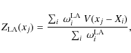
where Xi is the Doppler coordinate of the centre of each spectral line and xj is the Doppler coordinate axis. The symbol
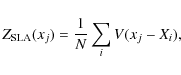
where SLA stands for simplified line addition.
Although initially it was only used for the circular state of polarisation, since the MZS resulting from line addition is model-independent, it can be applied equally to Stokes I, Q, U or V. The reason is that no assumptions have been made in order to compute the MZS, being just the brute force line addition. Therefore, the line addition is a very powerful and robust method to detect Zeeman signatures in stellar polarised spectra where the signal-to-noise ratio per individual spectral line is very poor.
2.2 Least-squares deconvolution
The LSD technique was introduced for the detection of Zeeman signatures in
stellar polarised spectra by Donati et al. (1997). They postulated
that, in a given observed Stokes spectrum, the shape of the local Zeeman signature in
circular polarisation is identical for all spectral lines. This means that individual
Stokes V profiles are assumed to correspond to a common basic
Zeeman signature that is modulated by a proportionality factor. This coefficient
is then fixed in the framework of the weak field approximation. In other words, they assume that
the magnetic field is weak enough so that the Zeeman splitting is negligible compared
to the Doppler width of the spectral line. As a consequence, the radiative transfer
equation can be solved analytically and it can be demonstrated that the Stokes V profile
is proportional to the derivative of the intensity profile (Sears 1913; Landi degl'Innocenti & Landolfi 2004). Following this approximation,
Donati et al. (1997) found that the proportionality factor,
![]() ,
i.e.,
just the product of the central
wavelength of the transition,
,
i.e.,
just the product of the central
wavelength of the transition, ![]() ,
the central depth of the line, di, and the effective Landé factor,
,
the central depth of the line, di, and the effective Landé factor, ![]() .
Donati et al. (1997) also normalised the weights to a mean value of 500 nm.
Based on all these assumptions, a particular MZS is extracted by means of
a least squares method from the observed spectrum.
.
Donati et al. (1997) also normalised the weights to a mean value of 500 nm.
Based on all these assumptions, a particular MZS is extracted by means of
a least squares method from the observed spectrum.
We note that
![]() and
and
![]() ,
although apparently
different, have a very similar behaviour. If the spectral line is assumed to be of Gaussian shape
whose width is dominated by thermal effects, it is possible to show that
,
although apparently
different, have a very similar behaviour. If the spectral line is assumed to be of Gaussian shape
whose width is dominated by thermal effects, it is possible to show that
![]() in general.
in general.
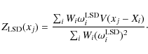
In more detail, the MZS obtained through the least-squares deconvolution method of Donati et al. (1997) is
calculated solving the following weighted linear regression problem: given N lines with Stokes Vprofiles
V(xj-Xi) sampled at the Nx Doppler coordinates xj, find the profile
Z(xj) that better approximates the observations in the least-squares sense
given the fixed values of
![]() .
In other words, it can be seen as the problem of fitting Nxindependent straight lines whose slopes are given by the values of Z(xj) and the
abscissae are the values of the weights
.
In other words, it can be seen as the problem of fitting Nxindependent straight lines whose slopes are given by the values of Z(xj) and the
abscissae are the values of the weights
![]() .
The solution is obtained, in the
case of Gaussian noise, by minimising the following merit functions:
.
The solution is obtained, in the
case of Gaussian noise, by minimising the following merit functions:
![\begin{displaymath}\chi^2_j = \sum_i W_i \left[V(x_j-X_i)-\omega_i^{\rm LSD} Z(x_j) \right]^2,
\end{displaymath}](/articles/aa/full_html/2009/36/aa10428-08/img24.png) |
(3) |
where the weights are usually chosen to be
![\begin{figure}
\center
\includegraphics[width=7.5cm,clip]{10428f1a.eps}\hspace*{3mm}
\includegraphics[width=8.1cm,clip]{10428f1b.eps}
\end{figure}](/articles/aa/full_html/2009/36/aa10428-08/img28.png) |
Figure 1:
Left panel: the probability distribution of the normalised LSD weights,
|
| Open with DEXTER | |
In combination with maximum entropy codes (Brown et al. 1991; Donati & Brown 1997), LSD-based Stokes I and V profiles have been used for the production of magnetic surface maps of quite a large number of stars with great success.
The main disadvantage of the LSD method relies on the assumptions made to obtain the MZS. It is not true in general that, locally, all spectral lines have a common shape (see for instance Kurucz 1993). Moreover, the weak field approximation used to obtain the proportionality coefficients states that Stokes Q and U are zero to first order. This would make this technique not applicable to recover the MZS of the linear states of polarisation.
2.3 Statistical properties of weights
A fundamental point to clarify is why LSD works even though it is based on assumptions
that seem unlikely. For this, we analyse the statistical properties of the weights. The left panel
of Fig. 1 presents the probability distribution function of the normalised weights
![]() for many lines in several line-lists obtained for different
stellar temperatures. We have verified that the distribution is relatively insensitive to
the value of the surface gravity and the only strong dependency is seen with respect
to the effective temperature. The histograms have been calculated for lines above 300 nm
and whose calculated line depth is larger than 0.4, which is the typical selection
criterion used in the standard application of LSD. The vertical lines in Fig. 1
are the value of the inverse of the number of lines included in the histograms, in other
words, the value of the weights in the simplest version of line addition given by
Eq. (2). Therefore,
the LSD weights can be considered, to a good approximation, to be positive random
variables whose distribution is close
to log-normal (which can be not approximately represented by a Gaussian distribution), centred around
1/N and with a certain dispersion. The log-normal shape arises
because the product of several independent random quantities converge towards
such a distribution, similar to the convergence towards a Gaussian distribution when
adding many independent quantities. In our case, the weights are the product of three quantities
which are largely independent.
for many lines in several line-lists obtained for different
stellar temperatures. We have verified that the distribution is relatively insensitive to
the value of the surface gravity and the only strong dependency is seen with respect
to the effective temperature. The histograms have been calculated for lines above 300 nm
and whose calculated line depth is larger than 0.4, which is the typical selection
criterion used in the standard application of LSD. The vertical lines in Fig. 1
are the value of the inverse of the number of lines included in the histograms, in other
words, the value of the weights in the simplest version of line addition given by
Eq. (2). Therefore,
the LSD weights can be considered, to a good approximation, to be positive random
variables whose distribution is close
to log-normal (which can be not approximately represented by a Gaussian distribution), centred around
1/N and with a certain dispersion. The log-normal shape arises
because the product of several independent random quantities converge towards
such a distribution, similar to the convergence towards a Gaussian distribution when
adding many independent quantities. In our case, the weights are the product of three quantities
which are largely independent.
The right panel of Fig. 1 presents a similar statistical analysis except
for line addition. In our study we use standard line-lists applied to LSD in which the
equivalent width is not present. For this reason, we plot the weights for the
simplifi the effective Landé factors of all
included lines, so that we plot the histogram of
![]() .
The
vertical lines again indicate the value of 1/N for each temperature. The weights
can again be represented approximately as Gaussian random variables centred around
1/N and with a certain dispersion.
.
The
vertical lines again indicate the value of 1/N for each temperature. The weights
can again be represented approximately as Gaussian random variables centred around
1/N and with a certain dispersion.
Assuming wavelength-independent Gaussian noise in the observations
characterised by a variance ![]() ,
the observed Stokes
V(xj-Xi) profiles can be
considered to be random variables characterised by a normal
distribution with a mean value of
,
the observed Stokes
V(xj-Xi) profiles can be
considered to be random variables characterised by a normal
distribution with a mean value of ![]() and variance
and variance ![]() .
In our case,
.
In our case,
![]() is the hidden Zeeman signature at Doppler coordinate xj that we want to recover.
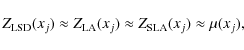
According to the results presented in Fig. 1,
the MZS of Eqs. (1) and (4) can be approximated
to be the addition of N products of two Gaussian random variables.
It is known that the probability distribution of the product
of two Gaussian random variables X and Y is, in general, very complex to calculate.
However, it is possible to obtain the mean and variances of such products
through the calculation of the moment generating function (Craig 1936):
is the hidden Zeeman signature at Doppler coordinate xj that we want to recover.
According to the results presented in Fig. 1,
the MZS of Eqs. (1) and (4) can be approximated
to be the addition of N products of two Gaussian random variables.
It is known that the probability distribution of the product
of two Gaussian random variables X and Y is, in general, very complex to calculate.
However, it is possible to obtain the mean and variances of such products
through the calculation of the moment generating function (Craig 1936):
where the
with variance
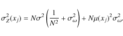
The signal-to-noise ratio increases roughly linearly with the number of added lines but reaches a maximum value at:
where
The previous results suggest the surprising possibility of using purely random weights in
the application of line addition or LSD. The only requisite is that the weights are
positive definite with a fairly symmetric distribution peaking close to 1/N with
a sufficiently small dispersion not to dominate in Eq. (7). Such
a distribution should lead to results similar to
those presented in Eqs. (6) and (7). Also surprising
is the fact that the analysis we have carried out suggests that the best solution is
to add the lines without any weight. In this case, no saturation due to the presence of
dispersion in the weights appears. This is a consequence of the fact that, since the
observations are assumed to be described by the Gaussian distribution
![]() ,
the maximum-likelihood estimation of its mean is exactly given by Eq. (2).
,
the maximum-likelihood estimation of its mean is exactly given by Eq. (2).
Summarising, one can consider that LSD and complex line addition schemes work because they give a response similar to that of the simplest line addition method. The fundamental reason is that spectral lines constitute a well-behaved statistical sample. The line-to-line differences are small enough (for instance, the dispersion in the value of the LSD or LA weights) so that the plain addition of lines makes the signal appear as soon as one adds a sufficient number of lines. Although the assumptions on which LSD or any method are based are not really fulfilled, the addition of lines dilutes any possible difference in their behaviour.
![\begin{figure}
\par\includegraphics[width=16.5cm,clip]{10428f2.eps}
\end{figure}](/articles/aa/full_html/2009/36/aa10428-08/img48.png) |
Figure 2:
Top panels: spectral synthesis of the 9 selected lines of the multiplet 816 of Fe I
(see Table 1; line 1 to 9 from left to right) having a spectral resolution of 3 |
| Open with DEXTER | |
3 The magnetic sensitivity of the MZS
The MZS are very efficient detectors of the magnetic activity of the star through of the Zeeman effect. However, since our main interest is to understand the magnetism of the stars, we need to infer the magnetic field vector of the star from the information contained in the polarised spectra or from the MZS. In cools stars the signal to noise ratio per individual spectral line is usually so poor that it is impossible to make reliable measurements of the magnetic field. Consequently, we are obliged to use the MZS as indicators of the magnetic activity in the stars. At this point a question arises: does the MZS contain the information on the magnetism of the star? It is evident that, in the case of line addition, the MZS is not a physical spectral line. Then, does it behave like a spectral line and contain any information about the magnetic field?. This section will be devoted to study to what extent it is possible to use the MZS to reliably infer the magnetic field in stars.
We simulate the observed spectral lines from a star assuming a Milne-Eddington
atmosphere. Moreover, we suppose that there is only one magnetic field vector in the
stellar surface that is responsible for the Zeeman signatures in the spectra.
Although more sophisticated scenarios and solutions to the polarised radiative transfer
equation exist, we are not interested in a realistic simulation of the stellar spectra
but rather in showing that, once the information of the spectra is encoded in the MZS, we are
capable of retrieving it. Using the M-E model facilitates the analysis and does not
require heavy calculations. We use the code Diagonal
as described in López Ariste & Semel (1999) with only one layer. For the sample M-E model atmosphere
we choose the value of the gradient of the source function to be
![]() and the ratio between the line and continuum absorption,
and the ratio between the line and continuum absorption, ![]() ,
to be equal to twice the relative strength of the
components of the multiplet as given by Allen (2000). Doppler broadening
is set to 21 mÅ as in sunspots, and the reduced damping is taken to be 0.01
,
to be equal to twice the relative strength of the
components of the multiplet as given by Allen (2000). Doppler broadening
is set to 21 mÅ as in sunspots, and the reduced damping is taken to be 0.01![]() .
.
We synthesise the Stokes vector of only a few spectral lines with a spectral
resolution close to 3 ![]() 106. We select the multiplet 816 of
Fe I (listed in Table 1) to ensure the validity of LS coupling
and the easy determination of Zeeman patterns, relative line strengths, etc. We then add
the Stokes parameters of all the spectral lines using unit weights [therefore, using
the simplified line addition of Eq. (2)] and subsequently reduce the spectral
resolution to stellar conditions, say 75 000, obtaining the MZS.
106. We select the multiplet 816 of
Fe I (listed in Table 1) to ensure the validity of LS coupling
and the easy determination of Zeeman patterns, relative line strengths, etc. We then add
the Stokes parameters of all the spectral lines using unit weights [therefore, using
the simplified line addition of Eq. (2)] and subsequently reduce the spectral
resolution to stellar conditions, say 75 000, obtaining the MZS.
Table 1: List of spectral lines of multiplet 816 of neutral iron.
3.1 MZS in circular polarisation
Figure 2 shows the synthetic Stokes I and V together with the MZS for the selected Fe I lines
for three different values of the magnetic field strength. We keep a high spectral resolution of 100 m/s,
i.e. a resolution of 3![]() 106 and then study the effect on the MZS of smoothing, bringing the resolution
down to 75 000, which corresponds to sampling with a step of about 4 km s-1.
106 and then study the effect on the MZS of smoothing, bringing the resolution
down to 75 000, which corresponds to sampling with a step of about 4 km s-1.
With very high spectral resolution, both Stokes I and Stokes V profiles change morphology and details depending on the field strength. In the case of 500 G, we do not detect a clear magnetic splitting in the Stokes I profiles. Also, the Stokes V profiles are all very similar, the only difference being a scale factor. This is a consequence of the fact that for 500 G, all spectral lines are in the weak field regime of the Zeeman effect, where the magnetic splitting is smaller than the Doppler width of the line. However, when the magnetic field increases, the Zeeman splitting becomes evident in the intensity profiles and the circular polarisation profiles abandon the shape-similarity regime. The anomalous dispersion terms are now important and show the typical reversal of polarities in the centre of the Stokes V profile. This has no counterpart in the weak-field approximation since anomalous dispersion is a high-order effect. Although the spectral lines are now out of the weak field regime, they have not still reached the strong field regime (where the Zeeman splitting is very large as compared to the Doppler width of the line).
Considering the MZS, in the weak field case (500 G), we see that, even in the high spectral resolution case, the shapes of the intensity and circular polarisation MZS also resemble the individual Stokes I and Stokes V profiles, respectively. When lowering the spectral resolution to the typical stellar one, the profiles are also similar in shape but the amplitude has decreased and the profiles are wider. Note that the MZS in circular polarisation matches almost perfectly with the derivative of the intensity profile. The reason is that since all the lines are in the weak-field regime and the derivative is a linear operation, the addition of derivatives equals the derivative of the addition of lines. This confirms that, in this case, the weak field regime is a good approximation.
When we leave the weak field regime, the MZS at high spectral resolution shows some distortions that are due to the different shapes of the individual Stokes V profiles (each line departs from the weak-field regime at different values of the magnetic field strength). When we decrease the spectral resolution to the stellar case, in the case of 1500 G we see that the MZS for circular polarisation is close to the derivative of the intensity MZS profile. This means that, even if the individual spectral lines are not in the weak field regime, the MZS for circular polarisation can be in this regime when lowering the spectral resolution. The reason behind this behaviour is that the width of the lines are increased when lowering the spectral resolution, thus extending the validity of the weak-field regime. Consequently, the weak field regime applies for larger magnetic fields in the circular polarisation MZS than in the individual spectral lines (typically up to 600-700 G in the visible part of the spectrum). However, this does not occur in the 2500 G case. The low resolution circular polarisation MZS already differs substantially from the derivative of the intensity MZS.
The MZS constructed with line addition are not simple spectral lines in the sense that they have no associated wavelength and are not characterised by specific atomic parameters such as the excitation potential. Moreover, in the more general case they do not even correspond to a particular chemical element, and no specific spectroscopic term is attached to them. However, the Zeeman signatures do not disappear in the MZS. We have seen that they are sensitive to the magnetic field, also having a weak field regime where the amplitude of the circular polarisation MZS scales with the derivative of the intensity MZS. For this reason, they can be used to extract information about the magnetic field, as we show in Sect. 4.
3.2 MZS in linear polarisation
![\begin{figure}
\includegraphics[width=6.4cm,clip]{10428f3a.ps}\hspace*{5mm}
\inc...
...3c.ps}\hspace*{5mm}
\includegraphics[width=6.4cm,clip]{10428f3d.ps}
\end{figure}](/articles/aa/full_html/2009/36/aa10428-08/img61.png) |
Figure 3: The MZS for a magnetic field strength of 1000 G ( left panels) and 3000 G ( right panels). Inside each panel, the intensity profile are shown at the top, the polarisation profiles are shown at the bottom, with Stokes V shown in dashed lines and Stokes Q in solid lines. High spectral resolution profiles are shown within thin lines, while the smeared low spectral resolution profiles are indicated with thick lines. |
| Open with DEXTER | |
We denote ![]() the angle between the magnetic field vector and the LOS and take it between
the angle between the magnetic field vector and the LOS and take it between ![]() and
and
![]() ,
the positive LOS component. If all directions have the
same probability, the average inclination angle is
,
the positive LOS component. If all directions have the
same probability, the average inclination angle is
![]() rad
rad
![]() .
Likewise, the
median angle is
.
Likewise, the
median angle is
![]() .
In other words, there are as many orientations
between
.
In other words, there are as many orientations
between ![]() and
and
![]() as between
as between
![]() and
and
![]() .
For the case of negative LOS longitudinal fields,
.
For the case of negative LOS longitudinal fields,
![]() ,
the results for
,
the results for
![]() and for
and for
![]() are deduced similarly. In conclusion,
are deduced similarly. In conclusion, ![]() is likely to
be nearly
is likely to
be nearly
![]() .
.
Figure 3 shows the MZS for the Stokes I, Q and V parameters computed
with a magnetic field strength of 1 kG and 3 kG and an inclination
![]() .
Note that, for high spectral resolutions the MZS for Stokes Q is approximately 0.7 times the MZS for Stokes V.
Stokes Q changes with wavelength twice as fast as Stokes V, so that
for current high spectral resolutions, say 75 000, Stokes Q shrinks much faster than Stokes V in the convolution
process. Moreover, Stokes Q changes sign when the azimuth changes by
.
Note that, for high spectral resolutions the MZS for Stokes Q is approximately 0.7 times the MZS for Stokes V.
Stokes Q changes with wavelength twice as fast as Stokes V, so that
for current high spectral resolutions, say 75 000, Stokes Q shrinks much faster than Stokes V in the convolution
process. Moreover, Stokes Q changes sign when the azimuth changes by
![]() ,
while Stokes V
changes sign when
,
while Stokes V
changes sign when ![]() changes by
changes by
![]() .
Both effects can be
reduced by increasing the spectral resolution, to values of the order of 120 000.
This means that observing at high spectral resolutions, Stokes Q is preserved considerably
and, more interestingly, the spatial resolution of the stellar surface is improved as well.
.
Both effects can be
reduced by increasing the spectral resolution, to values of the order of 120 000.
This means that observing at high spectral resolutions, Stokes Q is preserved considerably
and, more interestingly, the spatial resolution of the stellar surface is improved as well.
4 Recovering the magnetic field from the MZS
Our purpose is to assess to what extent the new MZS still contains all the information on the magnetic field that was present in the individual spectral lines in our sample. To this end, we examine the invariants that we had already found in solar magnetism, like the displacement of the centre of gravity (CoG) that yields a good approximation to the longitudinal component of the magnetic field. It is important to have in mind that the centre of gravity is a linear operator and commutes with the algebra of line addition and with smoothing.
The centre of gravity method applies only to circular polarisation; it is well studied in solar magnetism and described in a number of papers such as Rees et al. (1979, and references therein). In the limiting case of optically thin layers in local thermodynamical equilibrium, the centre of gravity shift of the line profiles observed in circular polarisation is proportional to the longitudinal component of the magnetic field. This still holds true, even for line formation in optically thick layers, in the limiting case of weak magnetic fields. Usually, this simple method is still a fair approximation in the more general case, but there are a few exceptions - see Semel (1967) for theoretical demonstrations, experimental tests and some exceptions. For further discussion of the CoG method applied to stars see also Stift (1986) and Leone & Catanzaro (2004).
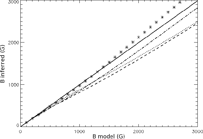 |
Figure 4:
Top: a test of the centre of gravity method. The CoG
shifts are calculated over a database of 30 values of magnetic fields in
steps of 100 Gauss from 0 to 3 kG. The shifts are divided by the cosine
of the inclination angle and by the adopted effective Landé factor to compare with
the amplitude of the magnetic field (abscissa). The curves are shown
for the following values of |
| Open with DEXTER | |
We apply the centre of gravity method to the MZS of Stokes V
(the ones shown in Fig. 2). We compute the MZS for Stokes V assuming
a magnetic field strength going from 0 to 3 kG having different inclinations
![]() and 80
and 80![]() .
Then, we infer the magnetic field
following the centre of gravity method. Figure 4 shows the plot
of the deduced magnetic field versus the theoretical one. The figure shows a clear linear trend
showing that the MZS contains the information of the magnetic field that was present in the
individual spectral lines. Since the centre of gravity is applicable both to the individual spectral lines and
to the MZS of Stokes V, we conclude that the MZS encodes the information of the magnetism of the
star in a similar way to how the individual spectral lines encode information. In other words,
the MZS constructed with the
line addition technique behaves as a spectral line although no specific atomic element is associated with it. However,
it can be characterised by an effective Landé factor and the extraction of the magnetic information
is possible. Figure 4 also shows an error close to 10% of the inferred value which is intrinsic to the
centre of gravity method. Our aim here is to show that the magnetic information is present in the MZS and not to
carry out precise measurements of the magnetic field strength. In order to perform these exact measurements, we must use
more sophisticated techniques. To have reliable values of the magnetic field, it is fundamental that the
inversion procedure uses the same operator O that generates the MZS
for the comparison with observational data. This
topic will be discussed in a forthcoming paper.
.
Then, we infer the magnetic field
following the centre of gravity method. Figure 4 shows the plot
of the deduced magnetic field versus the theoretical one. The figure shows a clear linear trend
showing that the MZS contains the information of the magnetic field that was present in the
individual spectral lines. Since the centre of gravity is applicable both to the individual spectral lines and
to the MZS of Stokes V, we conclude that the MZS encodes the information of the magnetism of the
star in a similar way to how the individual spectral lines encode information. In other words,
the MZS constructed with the
line addition technique behaves as a spectral line although no specific atomic element is associated with it. However,
it can be characterised by an effective Landé factor and the extraction of the magnetic information
is possible. Figure 4 also shows an error close to 10% of the inferred value which is intrinsic to the
centre of gravity method. Our aim here is to show that the magnetic information is present in the MZS and not to
carry out precise measurements of the magnetic field strength. In order to perform these exact measurements, we must use
more sophisticated techniques. To have reliable values of the magnetic field, it is fundamental that the
inversion procedure uses the same operator O that generates the MZS
for the comparison with observational data. This
topic will be discussed in a forthcoming paper.
5 Conclusions and discussion
We have used the line addition technique to show how to extract a Zeeman signature for any of the Stokes parameters. These technique, apart from being applicable to any state of polarisation, is also model independent. In other words, we do not need to adopt any approximation/assumption on the magnetic field or the stellar atmosphere to extract the Zeeman signature from the spectra. The line addition, as simple as the addition of many spectral lines, is a powerful tool to detect the magnetic field in cool stars, where the Zeeman signature per spectral line is very poor.
Moreover, the MZS created by the line addition technique also contains the magnetic information on the star. Therefore, it is possible to infer the magnetic (and the thermodynamical) properties of the stellar atmosphere using the appropriate inversion procedures. We have shown that the magnetic field strength can be inferred from the MZS of Stokes V by using a procedure as simple as the centre of gravity method. However, in order to have more reliable measurements of the magnetic field vector, we need to apply more sophisticated inversion procedures. Such procedures should ideally take into account the same operator used to create the MZS when comparing with observations.
Linear polarisation is often neglected in stellar polarimetry, under
the assumption that it will present amplitudes too small to
be observed. In this paper, we have demonstrated that, at
appropriate spectral resolutions, the linear polarisation due to the Zeeman
effect produces measurable signatures useful as diagnostics of the stellar magnetic fields.
With a resolution above 105, we can probably detect significant
signals in linear polarisation in the spectra of solar type stars.
Such a resolution has been achieved in spectroscopic tests with the SemPol instrument working
together with UCLES at the AAT with the 79 G/mm grating![]() .
The detection of linear polarisation in the spectrum
of a solar type star was carried out in 2004 (see Semel et al. 2006). The
linear signal observed was indeed four times less than the circular one,
but still significant. There is definitely an interest of using this method.
.
The detection of linear polarisation in the spectrum
of a solar type star was carried out in 2004 (see Semel et al. 2006). The
linear signal observed was indeed four times less than the circular one,
but still significant. There is definitely an interest of using this method.
We have also demonstrated why line addition and least-squares deconvolution give very similar MZS. The fundamental reason is that the weights used in both cases have well-defined statistical properties: their probability distribution is positive definite, centred at the inverse of the number of lines and not too broad. These properties cause that weighted line addition and LSD to converge to the simplest possible line addition which, since noise is assumed to be Gaussian, turns out to be the maximum-likelihood estimation of the MZS. This opens the curious possibility of applying LSD with random weights, provided they fulfil the mentioned properties.
In this paper we have presented a very simple technique to build the MZS. However, more powerful techniques are being developed using PCA. The main idea is to build a more sophisticated operator than the simple Dirac functions used for the line addition. The operator using PCA will be related to the eigenvectors of a database containing theoretical stellar spectra synthesised in several magnetic and thermodynamic configurations. Ramirez Vélez et al. (2009, submitted) explains this technique in detail and apply recent solar inversion procedures to the synthesised MZS using PCA. Other applications of PCA to obtain the MZS have been presented by Martínez González et al. (2008) and by Carroll et al. (2007). Application of PCA has been proven to be very effective in solar magnetometry and, analogously to the solar case, a database will be created and the PCA eigenvectors derived, applying the PCA-ZDI detection to just one magnetic point on the star. In later stages of the work, we shall discuss how to apply our approach to a few points on the stellar disc that are well separated by significant Doppler effects and treat the more realistic case of continuous distributions of fields over the stellar surface. Here, the orthogonality of the eigenvectors is not conserved for adjacent stellar points (that is, for small differences in the Doppler shifts).
Acknowledgements
Dr. David Rees has introduced PCA methods to the field of solar magnetometry which was the starting point for this method in general magnetometry including solar type stars. M. Semel wishes to express his gratitude to Dr. David Rees for lectures on PCA given during his visit to Meudon Observatory in 2002. We thank the referee, Prof. J. Landstreet, for many valuable comments that helped improve the paper. Our thanks go to Prof. S. Cuperman for reading the paper and for very precious comments and corrections. M.J.S. acknowledges support by the Austrian Science Fund (FWF), project P16003-N05 ``Radiation driven diffusion in magnetic stellar atmospheres'' and through a Visiting Professorship at the Observatoire de Paris-Meudon and Université Paris 7 (LUTH). M.J.M.G. and A.A.R. acknowledges finantial support by the Spanish Ministry of Education and Science through project AYA2007-63881. A.A.R. also acknowledges the European Commission through the SOLAIRE network (MTRN-CT-2006-035484).
References
- Allen, C. W. 2000, Astrophysical Quantities (New York: Springer Verlag and AIP Press) (In the text)
- Carroll, T. A., Kopf, M., Ilyn L., & Strassmmeier K. G. 2007, Astron. Nachr., 88, 789. (In the text)
- Brown, S. F., Donati, J.-F., Rees, D. E., & Semel, M. 1991, A&A, 250, 463 [NASA ADS] (In the text)
- Craig, C. C. 1936, Ann. Math. Statist., 7, 1 [CrossRef] (In the text)
- Donati, J.-F., & Brown, S. F. 1997, A&A, 326, 1135 [NASA ADS] (In the text)
- Donati, J.-F., Semel, M., Carter, B. D., Rees, D. E., & Collier Cameron, A. 1997, MNRAS, 291, 658 [NASA ADS] (In the text)
- Kurucz, R. L. 1993, Phys. Scr. T, 47, 110 [NASA ADS] [CrossRef] (In the text)
- Landi degl'Innocenti, & Landolfi, M. 2004, Polarization in Spectral Lines (Dordrecht: Kluwer Academic Publishers) (In the text)
- Leone F., & Catanzaro, G. 2004, A&A, 425, 271 [NASA ADS] [CrossRef] [EDP Sciences] (In the text)
- López Ariste, A., & Semel M. 1999, A&AS, 139, 417 [NASA ADS] [CrossRef] [EDP Sciences] (In the text)
- Martínez González, M. J., Asensio Ramos, A., Carroll, T. A., et al. 2008, A&A, 486, 637 [NASA ADS] [CrossRef] [EDP Sciences]
- Rees, D. E., & Semel, M. D. 1979, A&A, 74, 1 [NASA ADS] (In the text)
- Rees, D. E., López Ariste A., Thatcher J., & Semel M. 2000, A&A, 355, 759 [NASA ADS]
- Sears F. H. 1913, ApJ, 38, 99 [NASA ADS] [CrossRef]
- Semel, M. 1967, A&A, 30, 257 (In the text)
- Semel, M. 1980, A&A, 91, 369 [NASA ADS]
- Semel, M. 1987, A&A, 178, 257 [NASA ADS]
- Semel, M. 1989, A&A, 225, 456 [NASA ADS] (In the text)
- Semel, M. 1995, in Tridimensional Optical Spectroscopic Methods in Astrophysics, ed. G. Comte, & M. Marcelin, ASP Conf. Ser., 71, 340 (In the text)
- Semel, M., & Li J. 1996, Sol. Phys., 164, 417 [NASA ADS] [CrossRef]
- Semel, M., Rees, D. E., Ramíirez, Vélez, J. C., Stift, M. J., & Leone F.-, in Solar Polarization 4, ed. R. Casini, & B. W. Lites, ASP Conf. Ser., 358, 355
- Stift, M. J. 1986, MNRAS, 221, 499 [NASA ADS] (In the text)
- Stift, M. J. 2000, COSSAM: Codice per la Sintesi Spettrale nelle Atmosfere Magnetiche, A Peculiar Newsletter, 33, 27
Footnotes
- ... 0.01
![[*]](/icons/foot_motif.png)
- Saturation has always been an important issue in solar and stellar magnetic field measurements. Here it is included in the procedure and we have to use the same procedure to treat inversion.
- ... grating
- See the discussion by López Ariste & Semel on the spectral resolution of UCLES in http://www.aao.gov.au/local/www/UCLES/cookbook/report2.html.
All Tables
Table 1: List of spectral lines of multiplet 816 of neutral iron.
All Figures
| |
Figure 1:
Left panel: the probability distribution of the normalised LSD weights,
|
| Open with DEXTER | |
| In the text | |
| |
Figure 2:
Top panels: spectral synthesis of the 9 selected lines of the multiplet 816 of Fe I
(see Table 1; line 1 to 9 from left to right) having a spectral resolution of 3 |
| Open with DEXTER | |
| In the text | |
| |
Figure 3: The MZS for a magnetic field strength of 1000 G ( left panels) and 3000 G ( right panels). Inside each panel, the intensity profile are shown at the top, the polarisation profiles are shown at the bottom, with Stokes V shown in dashed lines and Stokes Q in solid lines. High spectral resolution profiles are shown within thin lines, while the smeared low spectral resolution profiles are indicated with thick lines. |
| Open with DEXTER | |
| In the text | |
| |
Figure 4:
Top: a test of the centre of gravity method. The CoG
shifts are calculated over a database of 30 values of magnetic fields in
steps of 100 Gauss from 0 to 3 kG. The shifts are divided by the cosine
of the inclination angle and by the adopted effective Landé factor to compare with
the amplitude of the magnetic field (abscissa). The curves are shown
for the following values of |
| Open with DEXTER | |
| In the text | |
Copyright ESO 2009
Current usage metrics show cumulative count of Article Views (full-text article views including HTML views, PDF and ePub downloads, according to the available data) and Abstracts Views on Vision4Press platform.
Data correspond to usage on the plateform after 2015. The current usage metrics is available 48-96 hours after online publication and is updated daily on week days.
Initial download of the metrics may take a while.