| Issue |
A&A
Volume 504, Number 3, September IV 2009
|
|
|---|---|---|
| Page(s) | 727 - 740 | |
| Section | Extragalactic astronomy | |
| DOI | https://doi.org/10.1051/0004-6361/200809945 | |
| Published online | 09 July 2009 | |
Cosmic star-formation history from a non-parametric inversion of infrared galaxy counts![[*]](/icons/foot_motif.png)
D. Le Borgne1,2,3 - D. Elbaz1 - P. Ocvirk1,4 - C. Pichon2,3
1 - CEA/Saclay, DSM/IRFU/SAp, 91191 Gif-sur-Yvette, France
2 - UPMC Univ. Paris 06, UMR7095, Institut d'Astrophysique de Paris, 75014 Paris, France
3 - CNRS, UMR7095, Institut d'Astrophysique de Paris, 75014 Paris, France
4 - Astrophysikalisches Institut Potsdam, An der Sternwarte 16,
14482 Potsdam, Germany
Received 10 April 2008 / Accepted 17 April 2009
Abstract
Aims. This paper aims at providing new conservative constraints on the cosmic star-formation (SF) history from the empirical modeling of recent observations in the mid and far infrared.
Methods. We present a new empirical method based on a non-parametric inversion technique. It primarily uses multi-wavelength galaxy counts in the infrared and sub-mm (15, 24, 70, 160, 850 ![]() m), and it does not require any redshift information. This inversion can be considered as a ``blind'' search for all possible evolutions and shapes of the infrared luminosity function of galaxies, from which the evolution of the star-formation rate density (SFRD) and its uncertainties are derived. The cosmic infrared background (CIRB) measurements are used a posteriori to tighten the range of solutions. The inversion relies only on two hypotheses: (1) the luminosity function remains smooth both in redshift and luminosity; (2) a set of infrared spectral energy distributions (SEDs) of galaxies must be assumed, with a dependency on the total luminosity alone.
m), and it does not require any redshift information. This inversion can be considered as a ``blind'' search for all possible evolutions and shapes of the infrared luminosity function of galaxies, from which the evolution of the star-formation rate density (SFRD) and its uncertainties are derived. The cosmic infrared background (CIRB) measurements are used a posteriori to tighten the range of solutions. The inversion relies only on two hypotheses: (1) the luminosity function remains smooth both in redshift and luminosity; (2) a set of infrared spectral energy distributions (SEDs) of galaxies must be assumed, with a dependency on the total luminosity alone.
Results. The range of SF histories recovered at low redshift is well-constrained and consistent with direct measurements from various redshift surveys. Redshift distributions are recovered without any input into the redshifts of the sources making the counts. A peak of the SFRD at ![]() is preferred, although higher redshifts are not excluded. We also demonstrate that galaxy counts at 160
is preferred, although higher redshifts are not excluded. We also demonstrate that galaxy counts at 160 ![]() m present an excess around 20 mJy that is not consistent with counts at other wavelengths under the hypotheses cited above. Finally, we find good consistency between the observed evolution of the stellar mass density and the prediction from our model of SF history.
m present an excess around 20 mJy that is not consistent with counts at other wavelengths under the hypotheses cited above. Finally, we find good consistency between the observed evolution of the stellar mass density and the prediction from our model of SF history.
Conclusions. Multi-wavelength counts and CIRB (both projected observations) alone, interpreted with a luminosity-dependent library of SEDs, contain enough information to recover the cosmic evolution of the infrared luminosity function of galaxies, and therefore the evolution of the SFRD, with quantifiable errors. Moreover, the inability of the inversion to model perfectly and simultaneously the multi-wavelength infrared counts implies either (i) the existence of a sub-population of colder galaxies; (ii) a larger dispersion of dust temperatures among local galaxies than expected; (iii) a redshift evolution of the infrared SED of galaxies.
Key words: galaxies: high-redshift - galaxies: evolution - Galaxy: formation - infrared: galaxies - submillimeter - galaxies: luminosity function, mass function
1 Introduction
Some key questions remain concerning the formation of galaxies, such as when and how galaxies formed their stars over the past 13 Gyr. Thanks to recent ultra-deep surveys at various wavelengths, some phenomena are now quite accurately measured and described, at least at relatively low redshift. For instance, it is well-established that massive galaxies have experienced most of their SF activity at early epochs, whereas the SF activity in small galaxies keeps a more constant level, on average. This so-called ``downsizing'' has been subject to many studies over the past few years (Madau et al. 1996; Steidel et al. 1999; Le Floc'h et al. 2005; Lilly et al. 1996; Juneau et al. 2005) and various signs of this downsizing are now seen. But precise measurements of the rate of stellar formation occurring at high redshift are still needed to efficiently challenge the latest models of galaxy formation. In other words, additional constraints on the modeling of the evolution of the cosmic SF history should be inspired by observations.
Recently, very deep surveys were designed to probe SF in the distant
universe. For instance, mid-infrared light (at 15 and 24 ![]() m) collected by the
ISO and Spitzer telescopes has been used extensively to measure the
star-formation rate (SFR) of both nearby and distant galaxies. The
evolution of the infrared (IR) luminosity functions (hereafter LF),
parameterized in shape (e.g. with Schechter functions), has
been measured up to z=2 with, again, a parameterization for the
evolution that can be both in luminosity (
m) collected by the
ISO and Spitzer telescopes has been used extensively to measure the
star-formation rate (SFR) of both nearby and distant galaxies. The
evolution of the infrared (IR) luminosity functions (hereafter LF),
parameterized in shape (e.g. with Schechter functions), has
been measured up to z=2 with, again, a parameterization for the
evolution that can be both in luminosity (
![]() )
or in
density (
)
or in
density (
![]() ). From these studies
(Caputi et al. 2007; Babbedge et al. 2006; Le Floc'h et al. 2005), several values of
). From these studies
(Caputi et al. 2007; Babbedge et al. 2006; Le Floc'h et al. 2005), several values of
![]() and
and
![]() have been measured in various redshift ranges and used to
derive the evolution of the SFRD. Such works give a
very solid basis to our understanding of galaxy evolution, but they
are generally limited to relatively low redshifts for two
reasons. First, they are very expensive in observation time if
spectroscopic redshifts are used to derive the luminosities of the
sources. Photometric redshifts can also be used to complement
spectroscopic redshifts, but their uncertainties are well-quantified
only at low redshift, where spectroscopic redshifts are available to
calibrate them. The second reason is that k-corrections of 24
have been measured in various redshift ranges and used to
derive the evolution of the SFRD. Such works give a
very solid basis to our understanding of galaxy evolution, but they
are generally limited to relatively low redshifts for two
reasons. First, they are very expensive in observation time if
spectroscopic redshifts are used to derive the luminosities of the
sources. Photometric redshifts can also be used to complement
spectroscopic redshifts, but their uncertainties are well-quantified
only at low redshift, where spectroscopic redshifts are available to
calibrate them. The second reason is that k-corrections of 24 ![]() m
light becomes large and hazardous at z>2 where the
restframe wavelength falls in the PAH features. The derivations of
total infrared luminosities and SFRs are
therefore uncertain. In the following, we call this approach ``direct
method'' and it consists in deriving luminosity functions
and SFRD from mid-IR light collected in redshift surveys.
m
light becomes large and hazardous at z>2 where the
restframe wavelength falls in the PAH features. The derivations of
total infrared luminosities and SFRs are
therefore uncertain. In the following, we call this approach ``direct
method'' and it consists in deriving luminosity functions
and SFRD from mid-IR light collected in redshift surveys.
However, these studies present some severe limitations.
First, a full multi-wavelength approach has not yet been used to measure
these quantities. Indeed, the studies cited above only use observations
in one mid-IR band to extrapolate to a total IR luminosity and derive an
SFR from uncertain calibrations (e.g. Kennicutt 1998).
Moreover, various depths and areas must be explored simultaneously.
On the one hand, only very deep surveys are able to probe
the lowest levels of SF in distant galaxies, which is necessary
to account for the total volume-average SF activity potentially
dominated by numerous galaxies with low SFRs. But these very deep surveys
necessarily probe only a small area in the sky. On the other hand, large (and therefore
shallow) surveys are also needed to probe the populations of
sources presenting a low density on the sky. It is the case for very
low-redshift sources and it might also be the case for the distant
populations of
ULIRGS![]() for instance.
for instance.
A natural way of exploiting this multi-wavelength and
multi-scale information all-together is to adopt a global modeling
approach. Ideally, the models (defined as the combination of a library
of IR SEDs and of an evolving LF) must be able to simultaneously account
for all the counts observed at all IR wavelengths, from
faint to bright sources. In addition, they must also account for the
constraints brought by measurements of the CIRB, and from LFs measured
with the ``direct method''. For instance, Chary & Elbaz (2001, hereafter CE01) and
Lagache et al. (2003, hereafter LDP03) or Franceschini et al. (2001) have found
models that
are able to reproduce most of these
constraints. However, some adjustments of the LFs or even of the SEDs
by these authors were needed to reproduce the most up-to-date
observations. This modeling approach is powerful but it is also
subject to caveats. Indeed, some important choices must be made for how
to parameterize the shape (e.g. a double power law, a Schechter function, or the local
15 ![]() m LF from Xu 2000, converted into
m LF from Xu 2000, converted into
![]() )
and the evolution of
the LFs (e.g. with factors
)
and the evolution of
the LFs (e.g. with factors
![]() and
and
![]() ). These parameterizations rely mainly on physical
intuition and sometimes require adding more degrees of freedom. This
is the case for the two populations of sources introduced by LDP03,
with their LFs evolving separately from each other. Moreover, these
models cannot claim to be the only possible representation of the true
cosmic LFs or of the true SEDs. They are generally good enough to reproduce
current observations, but they are never provided with a range of
uncertainties.
). These parameterizations rely mainly on physical
intuition and sometimes require adding more degrees of freedom. This
is the case for the two populations of sources introduced by LDP03,
with their LFs evolving separately from each other. Moreover, these
models cannot claim to be the only possible representation of the true
cosmic LFs or of the true SEDs. They are generally good enough to reproduce
current observations, but they are never provided with a range of
uncertainties.
In this paper, we add new constraints to the decomposition of the ``Lilly-Madau'' SFRD diagram using a powerful non-parametric inversion technique that blindy and simultaneously exploits the information from the published multi-wavelength IR galaxy counts in deep and small, as well as large and shallow, surveys. From these counts alone, and without any input information on redshifts, we derive the range of all possible evolutions and shapes of the IR LF.
In Sect. 2, we present the inversion method in
the general case (see also Appendix A). We present in
Sect. 3 the data and our choice for an SED
library used in this study. Sect. 4 contains our
results: the counts inversion and the corresponding IR LFs, together
with the inferred cosmic SF history. In
Sect. 5, we validate our inversion by comparing
our empirical modeling of counts, LFs, SFRD, and stellar-mass density
evolution to bibliographic data (see also
Appendix B for the robustness of the inversion).
Finally, we discuss the results and give our conclusions in
Sect. 6. Some predictions for forthcoming
Herschel observations are also given in
Appendix C. We use a
cosmology defined by H0= 70 km s-1 Mpc-1,
![]() ,
,
![]() .
The IMF is assumed to be Salpeter (1955) unless
otherwise stated (i.e. in Sect. 5.4).
.
The IMF is assumed to be Salpeter (1955) unless
otherwise stated (i.e. in Sect. 5.4).
2 Method: non-parametric inversion of deep multi- IR galaxy counts
In this section, we present a new approach to infer the evolution of IR
LFs of galaxies from multi-wavelength and multi-scale observations of
galaxy counts.
It consists in a phenomenological modeling approach, similar to the
works of CE01, LDP03, and others![]() .
However, the modeling is made here in a global and flexible way:
assuming that a given library of SEDs is able to account for the
spectra of galaxies at any redshift (an assumption tested
from the limits of the method's success), we search blindly for all
shapes and evolutions of the total IR LF that are able to reproduce
the multi-wavelength IR counts and the CIRB. This method is
non-parametric; i.e., it does not depend on a parameterization
of the LF (in shape or evolution). It must be noted, however,
that the underlying model of SEDs (on which the inversion depends) can,
itself, involve one or several parameters that must be fixed for the inversion.
.
However, the modeling is made here in a global and flexible way:
assuming that a given library of SEDs is able to account for the
spectra of galaxies at any redshift (an assumption tested
from the limits of the method's success), we search blindly for all
shapes and evolutions of the total IR LF that are able to reproduce
the multi-wavelength IR counts and the CIRB. This method is
non-parametric; i.e., it does not depend on a parameterization
of the LF (in shape or evolution). It must be noted, however,
that the underlying model of SEDs (on which the inversion depends) can,
itself, involve one or several parameters that must be fixed for the inversion.
Our method exploits data from infrared surveys designed to probe
high-redshift populations by using their observed galaxy number
counts. However, the redshifts of the sources are not required, which
makes this method quite versatile![]() .
.
An important advantage of this technique, one that makes it different from all previous models for IR galaxy number counts, is that it provides an automatic, hence objective, way of sampling the range of possible histories of the IR luminosity function. While previous studies have always presented their favorite model for fitting the IR galaxy counts, the present work spans the range of all possible evolutions that are consistent with the observations. This results in two major improvements. First, the modeled cosmic SFR history or luminosity functions per redshift bin are presented with their error bars. Second, it will allow us to discuss the limitation of local IR SEDs at reproducing the properties of distant galaxies. Indeed, if after spanning all possibilities, we still find that the fit is not complete, this will demonstrate that the IR SEDs must be revised, either because they provide an incomplete description of local galaxies or because they evolve with redshift.
In this section, as well as in Appendix A, we present the technical and mathematical aspects of our counts modeling.
2.1 Linear matrix modeling of the counts
The deep galaxy counts can be seen as the projection on a flux scale
of the SEDs of galaxies of various luminosities, masses, types,
etc., distributed in redshift. Therefore, to reproduce counts, one
needs at least a description of the number of galaxies at
various redshifts per unit volume, the
SEDs of these galaxies![]() , and a cosmology.
, and a cosmology.
In the following, to describe the numbers of galaxies in space and
time, we use total infrared luminosity functions (LF![]() ). Doing so,
we simultaneously assume that the SED of a galaxy seen in the IR can
be efficiently described by the sheer knowledge of its redshift and
). Doing so,
we simultaneously assume that the SED of a galaxy seen in the IR can
be efficiently described by the sheer knowledge of its redshift and
![]() .
Although such a description can be regarded as simple-minded,
the current knowledge of galaxy SEDs in the IR is not much better than
an empirical description parameterized only by
.
Although such a description can be regarded as simple-minded,
the current knowledge of galaxy SEDs in the IR is not much better than
an empirical description parameterized only by
![]() .
Therefore, the model
description that we have chosen is suited to the current limitations of our
understanding.
.
Therefore, the model
description that we have chosen is suited to the current limitations of our
understanding.
For a galaxy (which IR SED is known) lying at redshift z0 with a
luminosity
![]() ,
we can easily compute a k-correction and a
distance modulus to obtain the flux density S0 that one would measure
in a given IR filter centered at the wavelength
,
we can easily compute a k-correction and a
distance modulus to obtain the flux density S0 that one would measure
in a given IR filter centered at the wavelength ![]() .
This
conversion only depends on the cosmology and on the SED of the galaxy.
.
This
conversion only depends on the cosmology and on the SED of the galaxy.
A luminosity function being only the description of the number of
sources per comoving Mpc3 as a function of redshift and infrared
luminosity
![]() ,
we can then compute a matrix that converts this
evolving LF
,
we can then compute a matrix that converts this
evolving LF![]() into numbers of galaxies seen at various fluxes and
through different IR filters. This matrix is simply the response
function of the conversion from
into numbers of galaxies seen at various fluxes and
through different IR filters. This matrix is simply the response
function of the conversion from
![]() to
to
![]() presented above. Again, this matrix depends only on the cosmology and
on the library of SEDs. Since it includes k-correction,
distance effects (dimming as a function of the square of the luminosity
distance), and redshift effects (flux density stretching and dimming),
we call it the ``k+d'' matrix in the
following
presented above. Again, this matrix depends only on the cosmology and
on the library of SEDs. Since it includes k-correction,
distance effects (dimming as a function of the square of the luminosity
distance), and redshift effects (flux density stretching and dimming),
we call it the ``k+d'' matrix in the
following![]() .
.
After discretization, and using a matrix notation, the inverse problem can be formalized as
where Y is the matrix containing the number counts at fluxes S in bands
Therefore, our problem involves inverting this linear equation to find
the evolving LFs (i.e. redshift dependent number counts per unit volume), X,
from the known values of Y (the wavelength dependent
observed number counts per unit area). Because the matrix, M, is not
square, and because the number counts are noisy and must be
positive, the solution is not quite as simple as using the pseudo
inverse:
![]() ,
and
requires computing a regularized solution as discussed bellow and
explained in Appendix A. The reader may also refer to, e.g.
Pichon et al. (2002) or Ocvirk et al. (2006b). The
uncertainties on the observed counts Y are taken into
account through an additional error matrix W that makes it
possible to compute a
,
and
requires computing a regularized solution as discussed bellow and
explained in Appendix A. The reader may also refer to, e.g.
Pichon et al. (2002) or Ocvirk et al. (2006b). The
uncertainties on the observed counts Y are taken into
account through an additional error matrix W that makes it
possible to compute a ![]() between the model X and the
data Y and to derive uncertainties on the recovered LF.
between the model X and the
data Y and to derive uncertainties on the recovered LF.
In this formalism, we choose to describe the luminosity
function in a logarithmic scale, taking ![]()
![]() instead of
instead of
![]() everywhere. This is justified by the better conditioning of
the inversion in this case because the LF
everywhere. This is justified by the better conditioning of
the inversion in this case because the LF![]() generally spans several
orders of magnitudes in luminosity. For the same reason, the counts
are treated numerically through their Euclidian differential form
generally spans several
orders of magnitudes in luminosity. For the same reason, the counts
are treated numerically through their Euclidian differential form
![]() (units of mJy1.5 deg-2) which varies
slowly with flux. The evolution is measured as a function of
(units of mJy1.5 deg-2) which varies
slowly with flux. The evolution is measured as a function of
![]() .
Indeed, in the following, we impose a smooth
evolution in redshift of the luminosity function and we need to define
the temporal parameter on which this smoothing applies. We find that
the simplest redshift description that corresponds roughly to a
regular time sampling is actually
.
Indeed, in the following, we impose a smooth
evolution in redshift of the luminosity function and we need to define
the temporal parameter on which this smoothing applies. We find that
the simplest redshift description that corresponds roughly to a
regular time sampling is actually
![]() .
A parameterization
with z or with
.
A parameterization
with z or with
![]() would leave too much room for
strong variations in LF
would leave too much room for
strong variations in LF![]() at early and late times, respectively.
More quantitatively, we discretize the problem in bins regular in
at early and late times, respectively.
More quantitatively, we discretize the problem in bins regular in
![]()
![]() = 0.1
and in
= 0.1
and in
![]() ,
which corresponds to the sampling that
is good enough to produce counts with regular flux sampling of
,
which corresponds to the sampling that
is good enough to produce counts with regular flux sampling of
![]() S=0.1.
S=0.1.
2.2 Regularizing the inverse problem
In practice, provided the number of bins in LF![]() is large enough,
this problem is ``ill-posed'': there is possibly a large
number of LFs that are able to satisfy Eq. (1) perfectly,
hence overfitting the noisy counts. However, many of these solutions
are unlikely and not physical so that we need to ``regularize'' the
problem to obtain valid solutions. The first natural constraint is
the positivity of the LF
is large enough,
this problem is ``ill-posed'': there is possibly a large
number of LFs that are able to satisfy Eq. (1) perfectly,
hence overfitting the noisy counts. However, many of these solutions
are unlikely and not physical so that we need to ``regularize'' the
problem to obtain valid solutions. The first natural constraint is
the positivity of the LF![]() (there are no such things as negative
numbers of galaxies). This imposes an iterative, CPU-costly approach
to the problem, and a choice for an initial guess (see below).
Moreover, we want to avoid solutions that are not meaningful given
our noisy finite set of counts, such as LFs that are chaotically
varying as a function of
(there are no such things as negative
numbers of galaxies). This imposes an iterative, CPU-costly approach
to the problem, and a choice for an initial guess (see below).
Moreover, we want to avoid solutions that are not meaningful given
our noisy finite set of counts, such as LFs that are chaotically
varying as a function of
![]() or redshift. Therefore, we penalize
the inversion with an extra term, added to the formal
or redshift. Therefore, we penalize
the inversion with an extra term, added to the formal ![]() ,
which
enforces the smoothness of the LF
,
which
enforces the smoothness of the LF![]() both in
both in
![]() and in z (see Appendix A and Ocvirk et al. 2006b, for the details of the
formalism). With these constraints, the
solutions, X (which depend on the choice of the initial
guess required for the nonlinear optimization), are reasonable and
can serve as a solid basis for future works. We can also optionally impose external
constraints as supplementary priors, namely the low-redshift luminosity
functions obtained from direct methods.
and in z (see Appendix A and Ocvirk et al. 2006b, for the details of the
formalism). With these constraints, the
solutions, X (which depend on the choice of the initial
guess required for the nonlinear optimization), are reasonable and
can serve as a solid basis for future works. We can also optionally impose external
constraints as supplementary priors, namely the low-redshift luminosity
functions obtained from direct methods.
To obtain the range of all realistic solutions for the nonlinear
optimization problem, we explore a wide range of random initial
guesses, in a Monte-Carlo approach with at least 100 realizations. The
range of LFs spanned by the initial guesses is much wider than the
range of the final LF![]() (X) obtained after convergence, which
lends credibility to our study's completeness
(X) obtained after convergence, which
lends credibility to our study's completeness![]() .
.
Finally, some of the solutions do not match the constraints brought by CIRB measurements. We filter out these invalid solutions, a posteriori, leaving only the most realistic luminosity functions.
3 Data and SEDs used in this work
3.1 Input multi-wavelength counts
![\begin{figure}
\par\includegraphics[width=17cm,clip]{09945f1.ps}
\end{figure}](/articles/aa/full_html/2009/36/aa09945-08/img34.png) |
Figure 1:
Observed 15/16 |
| Open with DEXTER | |
The multi-wavelength counts that we invert in this work are presented
in Fig. 1. They summarize bibliographic observed
galaxy counts at 15, 24, 70, 160, and 850 ![]() m. This compilation is
not exhaustive but we retained significant surveys for each
IR band, mixing wide and shallow ones to avoid cosmic variance effects
as much as possible, and deep ones for faint source detections. The
data shown in Fig. 1 are actual observations,
except for the 70 and 160
m. This compilation is
not exhaustive but we retained significant surveys for each
IR band, mixing wide and shallow ones to avoid cosmic variance effects
as much as possible, and deep ones for faint source detections. The
data shown in Fig. 1 are actual observations,
except for the 70 and 160 ![]() m points from Dole (private
communication; and also Dole et al. 2006), which are obtained from
stacking 24
m points from Dole (private
communication; and also Dole et al. 2006), which are obtained from
stacking 24 ![]() m sources in several flux bins and using an MIR-FIR
observed correlation. Although these points are not strict
measurements, the MIR-FIR relationship is tight enough (down to less
than 0.1 mJy) to be confident in the stacking results. We group the
15 and 16
m sources in several flux bins and using an MIR-FIR
observed correlation. Although these points are not strict
measurements, the MIR-FIR relationship is tight enough (down to less
than 0.1 mJy) to be confident in the stacking results. We group the
15 and 16 ![]() m counts, as well as the 160/170
m counts, as well as the 160/170 ![]() m counts, thus
neglecting the small differences to the counts (a few percent) that
are caused by the slightly different k-corrections. Our inversion is
applied to this compilation.
m counts, thus
neglecting the small differences to the counts (a few percent) that
are caused by the slightly different k-corrections. Our inversion is
applied to this compilation.
3.2 Library of SEDs
The IR SEDs that we use in this study are taken from the empirical library of CE01,
which defines a bijection between
![]() and the IR SED from 3 to 1000
and the IR SED from 3 to 1000
![]() m. Although this library is based on correlations observed in local
galaxies, we suppose in the following that the SEDs of galaxies with a
given
m. Although this library is based on correlations observed in local
galaxies, we suppose in the following that the SEDs of galaxies with a
given
![]() do not change with redshift. It does not necessarily mean
that SEDs of individual galaxies do not evolve, but that they must evolve along the local SED-
do not change with redshift. It does not necessarily mean
that SEDs of individual galaxies do not evolve, but that they must evolve along the local SED-
![]() correlation. It is worth noting that when a description of the evolving IR SEDs of
galaxies becomes available (e.g. with Herschel), the technique
that we use can be applied to these evolving SED libraries.
correlation. It is worth noting that when a description of the evolving IR SEDs of
galaxies becomes available (e.g. with Herschel), the technique
that we use can be applied to these evolving SED libraries.
Moreover, we ``clip'' this library for the highest IR
luminosities, using the
![]() = 1012.2
= 1012.2 ![]() SED shape for
galaxies more luminous than this value. This makes the SEDs colder
than in CE01 for ULIRGs and makes it compatible with most of the known
data, from low-redshift, low-luminosity to high-redshift luminous
galaxies (see CE01; Papovich et al. 2007). Figure 2
presents the relation between 24
SED shape for
galaxies more luminous than this value. This makes the SEDs colder
than in CE01 for ULIRGs and makes it compatible with most of the known
data, from low-redshift, low-luminosity to high-redshift luminous
galaxies (see CE01; Papovich et al. 2007). Figure 2
presents the relation between 24 ![]() m and total IR
luminosities that is predicted by the ``clipped'' CE01 library, together with
observations from (Papovich et al. 2007) in the range
z=1.5-2.5.
This clipping can be justified by the SEDs of high
luminosity galaxies (ULIRGs) like those seen at high redshift being
poorly known in the local universe: their dust temperature can only
be measured by Herschel. Therefore, the CE01 SEDs are extrapolated
within this luminosity range. We chose to clip the IR dust temperatures of
the CE01 library to those of the luminosity range really observed in
the local universe, rather than extrapolating them.
m and total IR
luminosities that is predicted by the ``clipped'' CE01 library, together with
observations from (Papovich et al. 2007) in the range
z=1.5-2.5.
This clipping can be justified by the SEDs of high
luminosity galaxies (ULIRGs) like those seen at high redshift being
poorly known in the local universe: their dust temperature can only
be measured by Herschel. Therefore, the CE01 SEDs are extrapolated
within this luminosity range. We chose to clip the IR dust temperatures of
the CE01 library to those of the luminosity range really observed in
the local universe, rather than extrapolating them.
![\begin{figure}
\par\includegraphics[width=8.9cm,clip]{09945f2.ps}
\end{figure}](/articles/aa/full_html/2009/36/aa09945-08/img36.png) |
Figure 2:
24 |
| Open with DEXTER | |
4 Results
In this section, we present the counts, luminosity functions, and SF history that are modeled from the counts inversion, as well as the effect of using or not using low-z luminosity functions as priors. We compare these results and their redshift decompositions to measurements obtained from direct methods and bibliographic data only in Sect. 5.
4.1 Counts inversion
![\begin{figure}
\par\includegraphics[width=17cm,clip]{09945f3.ps}
\end{figure}](/articles/aa/full_html/2009/36/aa09945-08/img37.png) |
Figure 3:
Mid- and Far-IR counts obtained from the non-parametric inversion of the
observed counts. The data counts that are the basis of the
inversion are represented by the shaded blue zones (fitted values |
| Open with DEXTER | |
This inversion model has been designed to reproduce infrared galaxy counts and as a result to derive a range of possible total IR LF as a function of redshift, that can be converted afterwards into a range of cosmic SF histories. The success of the model can be visually tested by comparing the range of predicted galaxy counts with the observed number counts and their dispersion (see Fig. 3).
At first glance, one can see that the observed counts are well-fitted over the
whole IR range, from 15 to 850 ![]() m. In particular, the bumps at 15
and 24
m. In particular, the bumps at 15
and 24 ![]() m are reproduced simultaneously. The 850
m are reproduced simultaneously. The 850 ![]() m differential
counts are well-fitted too: negative k-corrections make it possible to
see a high-redshift population of galaxies, namely ULIRGS and HLIRGS
(
m differential
counts are well-fitted too: negative k-corrections make it possible to
see a high-redshift population of galaxies, namely ULIRGS and HLIRGS
(
![]()
![]() )
at z>2, which are hardly seen at other
wavelengths except in faint 24 and 70
)
at z>2, which are hardly seen at other
wavelengths except in faint 24 and 70 ![]() m counts.
m counts.
Interestingly, one can see from Fig. 3 that, while
the only strong constraint that is imposed on the model is to keep a smooth
dependence of the LF with redshift and luminosity, the model is unable
to perfectly fit the observed number counts and their dispersion at
all flux densities and wavelengths even though the whole range of
possible LF and associated redshift evolution has been spanned
blindly. Some solutions tend not to fit the 15 ![]() m
counts perfectly, the 70
m
counts perfectly, the 70 ![]() m counts are slightly overproduced, and more
strikingly, the 160
m counts are slightly overproduced, and more
strikingly, the 160 ![]() m counts are underproduced around 20 mJy.
m counts are underproduced around 20 mJy.
A major strength of this model is to provide an
objective and statistically significant way to test a given library of
template SED. Indeed, the discrepancy between the model and observed counts
cannot arise from the LF itself since it was allowed to vary both with
luminosity and redshift with a high degree of freedom (see
also Ocvirk et al. 2006a, for a discussion on the corresponding biases in a slightly
different context). It must therefore arise from the library
of template SEDs that is used as an input for fitting the number counts
(through the ``k+d'' matrix M). The CE01 library of template
SEDs that is used here reflects the median trend of local galaxies and
was found to be statistically consistent with the radio-infrared
correlation up to ![]() (Appleton et al. 2004; Elbaz et al. 1999), with the mid-infrared observations of galaxies up to
(Appleton et al. 2004; Elbaz et al. 1999), with the mid-infrared observations of galaxies up to
![]() with moderate variations (Marcillac et al. 2006) and with massive galaxies selected with the BzK technique (Daddi et al. 2007b). The origin of the discrepancy can therefore come from
three possible origins. The first two possibilities compatible with no
evolution of the infrared SED of galaxies are (i) a
bias towards cold galaxies due to the shallow depth at 160
with moderate variations (Marcillac et al. 2006) and with massive galaxies selected with the BzK technique (Daddi et al. 2007b). The origin of the discrepancy can therefore come from
three possible origins. The first two possibilities compatible with no
evolution of the infrared SED of galaxies are (i) a
bias towards cold galaxies due to the shallow depth at 160 ![]() m
within the dispersion already existing at
m
within the dispersion already existing at ![]() ;
(ii) the existence
of a subpopulation of cold galaxies, already present locally but not
yet identified due to limited constraints on both sides of the peak
emission in the far infrared. A third possibility would be that the
infrared SEDs of galaxies evolve as a function of redshift (see e.g. Chapman et al. 2002).
;
(ii) the existence
of a subpopulation of cold galaxies, already present locally but not
yet identified due to limited constraints on both sides of the peak
emission in the far infrared. A third possibility would be that the
infrared SEDs of galaxies evolve as a function of redshift (see e.g. Chapman et al. 2002).
It is not possible to disentangle between the three possibilities
based on the present dataset. However, a forthcoming paper will study
this issue in detail using a stacking analysis at 160 ![]() m
(Magnelli et al., in preparation). It must be noted though that the
method described here is versatile enough to allow its user to test
any library of template SED against existing constraints from galaxy
counts and the infrared background. It will therefore be
a straightforward matter to check whether any change or evolution in the SEDs can reproduce
the number counts at all wavelengths and flux densities. We refrained
from making these adjustments to the counts at this stage since any of
the previously mentioned alternatives is equally possible.
m
(Magnelli et al., in preparation). It must be noted though that the
method described here is versatile enough to allow its user to test
any library of template SED against existing constraints from galaxy
counts and the infrared background. It will therefore be
a straightforward matter to check whether any change or evolution in the SEDs can reproduce
the number counts at all wavelengths and flux densities. We refrained
from making these adjustments to the counts at this stage since any of
the previously mentioned alternatives is equally possible.
4.2 Solutions: range of evolving luminosity functions
![\begin{figure}
\par\includegraphics[width=17cm,clip]{09945f4.ps}
\end{figure}](/articles/aa/full_html/2009/36/aa09945-08/img42.png) |
Figure 4:
All possible solutions for the evolving LFs that best reproduce
all the IR counts of Fig. 3 and the CIRB
constraints. As in Fig. 3, the thick red line and
the dashed red areas represent the best-fitting solution and the range of
allowed solutions, respectively. By construction, no conclusion on the
LF can be made in the vertical gray-shaded areas where a divergence is
expected because these objects are not seen in the counts because of the flux limits of
current IR surveys. At the top of each panel, the ranges of
|
| Open with DEXTER | |
Looking now at the main output of the model, i.e. the evolution of the
total IR luminosity function with redshift, we note that large parts
of the LF are constrained very well by the inversion (see Fig. 4). In
particular, the number density of galaxies with
![]() at z<0.5 is tightly constrained, as are
the numbers of galaxies with higher luminosities at higher redshift.
at z<0.5 is tightly constrained, as are
the numbers of galaxies with higher luminosities at higher redshift.
We will present in Sect. 5.2 a comparison of these
solutions to the LF![]() s obtained from direct measurements at low redshift.
s obtained from direct measurements at low redshift.
But before doing so, we note that a fraction of the solutions present a knee in
the LF, particularly at 0.3<z<1 around
![]() ,
which
is partly responsible for the bump seen in the number counts at 24 and
15
,
which
is partly responsible for the bump seen in the number counts at 24 and
15 ![]() m at the corresponding flux densities. However, not all
solutions of the inversion technique present such a strong knee, which
might be seen as an artifact.
m at the corresponding flux densities. However, not all
solutions of the inversion technique present such a strong knee, which
might be seen as an artifact.
4.3 Evolution of the star-formation activity
![\begin{figure}
\par\includegraphics[width=12.8cm,clip]{09945f5.ps}
\end{figure}](/articles/aa/full_html/2009/36/aa09945-08/img45.png) |
Figure 5: Star-formation rate density since z=5 derived from the counts inversions. The SFRD is obtained from the range of all possible luminosity functions derived from the counts and respecting the CIRB constraints. The solid lines correspond to the best fit to the counts and the transparent shaded areas show the range of uncertainties. From top to bottom at z=0.8: black = all galaxies, green = LIRGS, blue = normal star-forming galaxies, orange = ULIRGS, red = HLIRGS. |
| Open with DEXTER | |
The SFRD can now be estimated from the LFs that were obtained from the counts
inversion. The total infrared LFs are integrated over the whole range of luminosities
down to 107 ![]() .
The resulting total infrared luminosity density
is then converted into a SFRD using formula (2)
(Kennicutt 1998):
.
The resulting total infrared luminosity density
is then converted into a SFRD using formula (2)
(Kennicutt 1998):
![\begin{displaymath}{\it SFR ~[M}_{\odot}~ {\rm yr}^{-1}]=1.72 \times 10^{-10} ~ L_{\rm
IR} ~[L_{\odot}].
\end{displaymath}](/articles/aa/full_html/2009/36/aa09945-08/img46.png)
Therefore, the regions shown in Fig. 5 effectively represent the range of all possible SF histories that are compatible with the multi-
This inversion shows that, indeed, an IR downsizing is at work:
``normal'' galaxies dominate the SFRD at low redshift (although the
contribution of ULIRGS and HLIRGS are poorly constrained in the
low-z range because they would correspond to bright and very rare
sources, not easily seen in the counts of current deep surveys). At z>0.8, LIRGS
dominate the SFRD, whereas the contribution of ULIRGS peaks at
![]() .
These results will be compared in detail to measurements from direct methods and
bibliographic data in Sect. 5.3.
.
These results will be compared in detail to measurements from direct methods and
bibliographic data in Sect. 5.3.
As mentioned before, it is also possible to use an additional prior
for the inversion: direct measurements of the 8 or 15 ![]() m LF below
z=2. Although subject to many caveats (e.g. the strong dependency
on the PAH modeling of the SEDs), they can be used as a prior to guide the
inversion, and at least constrain the solutions at
low redshift
m LF below
z=2. Although subject to many caveats (e.g. the strong dependency
on the PAH modeling of the SEDs), they can be used as a prior to guide the
inversion, and at least constrain the solutions at
low redshift![]() .
.
We checked the effect of using this prior from direct measurements at
low redshift. We observe that some uncertainties in the LIRGS and
ULIRGS contributions are slightly tightened, but we also note that
the trends are basically unchanged. We interpret this surprising result as
follows: the leverage that we have access to by inverting galaxy
counts on a very wide wavelength-basis (from 15 to 850 ![]() m) is large
enough to provide a realistic description of the redshift distribution
of the sources on a statistical basis. This is likely to only be possible
because the library of SEDs that we use seems close to the real SEDs
of galaxies, on average (again, in the statistical sense) at any
redshift lower than
m) is large
enough to provide a realistic description of the redshift distribution
of the sources on a statistical basis. This is likely to only be possible
because the library of SEDs that we use seems close to the real SEDs
of galaxies, on average (again, in the statistical sense) at any
redshift lower than ![]() ,
thus avoiding a complete blurring of
the de-projection of multi-wavelength galaxy counts onto the
luminosity function space. Therefore, various populations of galaxies
at different redshifts are seen at various wavelengths, which
considerably reduces degeneracies and enables us to recover the history of IR
galaxies as a whole.
,
thus avoiding a complete blurring of
the de-projection of multi-wavelength galaxy counts onto the
luminosity function space. Therefore, various populations of galaxies
at different redshifts are seen at various wavelengths, which
considerably reduces degeneracies and enables us to recover the history of IR
galaxies as a whole.
Since the philosophy of this paper is to remain as conservative as possible, we choose not to use the low-redshift LF measured from direct methods as a prior in the following. Indeed, doing so would only slightly change our results, and it would introduce a source of potential additional errors propagating from the errors intrinsic to direct methods (k-corrections in the mid-infrared or redshifts).
5 Validation: comparison with direct measurements at low redshift
After presenting the global outputs of the model in the previous section, we detail here the redshift decomposition of the inversion results and we compare them to measurements obtained from direct (redshift-based) methods. This comparison is particularly challenging since no redshift information was used as an input in the inversion.
5.1 Redshift decomposition of the mid-IR counts
![\begin{figure}
\par\includegraphics[width=16cm,clip]{09945f6.ps}
\end{figure}](/articles/aa/full_html/2009/36/aa09945-08/img51.png) |
Figure 6:
Top and bottom left: counts at 16, 24, and 70 |
| Open with DEXTER | |
To validate our inversion results, we need to compare the redshift
decomposition of the IR counts to observations from a direct method.
To do so, we compared our results to data from the GOODS survey
(P.I. Dickinson for GOODS-Spitzer, P.I. M.Giavalisco for GOODS-HST)
originally presented in Giavalisco et al. (2004). This survey consists of two
fields which have been subject to several studies at various
wavelengths in the past few years. We investigated the redshift
decomposition of the counts at 16, 24, and 70 ![]() m using the optical
counterparts of these sources in GOODS and making use of the
spectroscopic and photometric redshifts. The sample that we used
covers a total area of 0.07 square degree on the sky. Although this
area is quite small and cosmic variance might affect our study, we
found that the luminosity functions measured from the direct method are
similar in both GOODS fields, making them compatible within
2
m using the optical
counterparts of these sources in GOODS and making use of the
spectroscopic and photometric redshifts. The sample that we used
covers a total area of 0.07 square degree on the sky. Although this
area is quite small and cosmic variance might affect our study, we
found that the luminosity functions measured from the direct method are
similar in both GOODS fields, making them compatible within
2![]() .
The spectroscopic completeness is high (60% at
.
The spectroscopic completeness is high (60% at
![]()
![]() Jy for z<1.5 sources), and we complemented them with
photometric redshifts computed with the code Z-Peg (Le Borgne & Rocca-Volmerange 2002)
with a precision
Jy for z<1.5 sources), and we complemented them with
photometric redshifts computed with the code Z-Peg (Le Borgne & Rocca-Volmerange 2002)
with a precision
![]() to 0.1 depending on the
redshift of the sources. We then used the
to 0.1 depending on the
redshift of the sources. We then used the
![]() formalism to correct
from incompleteness at the lower flux limit. The galaxies showing
signs of AGNs (identified from X-rays or optical emission lines), were
excluded from the sample of 24
formalism to correct
from incompleteness at the lower flux limit. The galaxies showing
signs of AGNs (identified from X-rays or optical emission lines), were
excluded from the sample of 24 ![]() m sources. Doing so enabled us to
use SEDs of galaxies to compute k-corrections and only
slightly affects our results, mainly at the very high-luminosity end of the
luminosity function at moderate (z=1) or high (z>2) redshifts.
m sources. Doing so enabled us to
use SEDs of galaxies to compute k-corrections and only
slightly affects our results, mainly at the very high-luminosity end of the
luminosity function at moderate (z=1) or high (z>2) redshifts.
Figure 6 presents the resulting comparison of the
redshift decomposition of the counts obtained from direct and inverse
methods. At 24 ![]() m, our best solution for the recovered LF
m, our best solution for the recovered LF![]() indeed
produces a redshift decomposition of the counts that is compatible
with the observed ones. The match of 15
indeed
produces a redshift decomposition of the counts that is compatible
with the observed ones. The match of 15 ![]() m counts as a function of
redshift is poorer because CE01 templates represent the
fluxes at this wavelength less well for 0.5<z<1 galaxies
(e.g. Marcillac et al. 2006). As for the 70
m counts as a function of
redshift is poorer because CE01 templates represent the
fluxes at this wavelength less well for 0.5<z<1 galaxies
(e.g. Marcillac et al. 2006). As for the 70 ![]() m counts, the observed
decomposition is not complete at faint fluxes, making the comparison
hazardous.
m counts, the observed
decomposition is not complete at faint fluxes, making the comparison
hazardous.
5.2 Comparison to direct measurements of the infrared luminosity functions
We now compare the range of luminosity functions LF![]() obtained from our inversion to
some measurements of the LF
obtained from our inversion to
some measurements of the LF![]() obtained from the direct method.
As noted before, several studies (Caputi et al. 2007; Babbedge et al. 2006; Le Floc'h et al. 2005)
have measured the 15 or 8
obtained from the direct method.
As noted before, several studies (Caputi et al. 2007; Babbedge et al. 2006; Le Floc'h et al. 2005)
have measured the 15 or 8 ![]() m luminosity functions, which can be
converted to LF
m luminosity functions, which can be
converted to LF![]() if a library of SEDs is assumed.
We show in Fig. 7 the results from (Le Floc'h et al. 2005)
for reference.
We also provide on the same figure our own direct measurements of the evolving
LF
if a library of SEDs is assumed.
We show in Fig. 7 the results from (Le Floc'h et al. 2005)
for reference.
We also provide on the same figure our own direct measurements of the evolving
LF![]() that we derived from 24
that we derived from 24 ![]() m galaxies seen in the GOODS fields
(North+South).
We chose to do these direct measurements again for two
reasons. First, for consistency with our inversion, we used the same
library of templates for the k-corrections (used for MIR to total LIR
conversion)
m galaxies seen in the GOODS fields
(North+South).
We chose to do these direct measurements again for two
reasons. First, for consistency with our inversion, we used the same
library of templates for the k-corrections (used for MIR to total LIR
conversion)![]() . Second, our data at 24
. Second, our data at 24 ![]() m reaches a depth of 24
m reaches a depth of 24 ![]() Jy
instead of 80
Jy
instead of 80 ![]() Jy in previous works, extending the LF to the
faint end. The completeness at this depth is 85% (Chary 2007).
Not surprisingly, our direct measurements of the LF
Jy in previous works, extending the LF to the
faint end. The completeness at this depth is 85% (Chary 2007).
Not surprisingly, our direct measurements of the LF![]() from 24
from 24 ![]() m
fluxes are compatible with previous studies that used the same
method. In particular, we find the same values as Le Floc'h et al. (2005)
who explored the z<1 domain. However, we reach higher redshift
galaxies thanks to the depth of our sample. However, k-corrections are very
uncertain for these high-z sources (24
m
fluxes are compatible with previous studies that used the same
method. In particular, we find the same values as Le Floc'h et al. (2005)
who explored the z<1 domain. However, we reach higher redshift
galaxies thanks to the depth of our sample. However, k-corrections are very
uncertain for these high-z sources (24 ![]() m corresponds to less than
8
m corresponds to less than
8 ![]() m at z>2, a range where the library of SEDs is not
validated). Therefore, we use these high-redshift measurements with
caution, as mentioned earlier.
m at z>2, a range where the library of SEDs is not
validated). Therefore, we use these high-redshift measurements with
caution, as mentioned earlier.
![\begin{figure}
\par\includegraphics[width=15.5cm,clip]{09945f7.ps}
\end{figure}](/articles/aa/full_html/2009/36/aa09945-08/img55.png) |
Figure 7:
Total IR luminosity functions derived independently
from the counts
inversion and from direct measurements. ``Clipped'' CE01 templates are used for the 24 |
| Open with DEXTER | |
It is striking in Fig. 7 that the LF obtained from the direct method is consistent with the best-fitting LF derived from the counts inversion in the common range that they probe. This is remarkable because no information on the redshift of the sources was used in the inversion. This means that all the constraints that one can get from these direct measurements are not really needed for the inversion: although we do not use the redshift of the sources, we recover the observed redshift distributions that are here expressed equivalently in terms of evolving luminosity functions. The interpretation is the same as for the redshift decomposition of the counts, which are different views of the same phenomenon.
The meaningfulness of the agreement between the observed and the
recovered LFs is strengthened by the fact that that both
![]() luminosity functions are measured or estimated using the same library
of SEDs, thus using the same k-correction in a consistent way. Using
another library of SEDs for both methods would produce the same kind
of agreement, although the precise shape of the LFs would be slightly
different from what we obtain here with the ``clipped'' CE01 library.
luminosity functions are measured or estimated using the same library
of SEDs, thus using the same k-correction in a consistent way. Using
another library of SEDs for both methods would produce the same kind
of agreement, although the precise shape of the LFs would be slightly
different from what we obtain here with the ``clipped'' CE01 library.
5.3 Cosmic star-formation history vs literature
In this section, we compare the SFRD history that we derived from the
multi-![]() counts inversion to ``direct'' measurements at low
redshift.
counts inversion to ``direct'' measurements at low
redshift.
5.3.1 Total SFRD
The comparison of the total SFRD derived with this inversion technique
matches the compilation of direct measurements from Hopkins & Beacom
(2006, Fig. 8).
Moreover, we also show in Fig. 8 the
SFRD that we derived from 24 ![]() m data in the GOODS fields. We must stress here that these measurements, obtained with
the ``direct'' method, are independent of the SFRD inferred by the
counts inversion
m data in the GOODS fields. We must stress here that these measurements, obtained with
the ``direct'' method, are independent of the SFRD inferred by the
counts inversion![]() . We only present them here for comparison to the
inversion results in this subsection. The total infrared luminosities measured for
individual 24
. We only present them here for comparison to the
inversion results in this subsection. The total infrared luminosities measured for
individual 24 ![]() m sources in the GOODS fields were summed up in redshift bins
and converted to SFRDs.
Like several authors before us
(e.g. Pérez-González et al. 2005; Flores et al. 1999; Le Floc'h et al. 2005), we could have
extrapolated the measured luminosity functions in the
faint end to obtain the total SFRD. But this is somewhat dangerous and depends strongly on the
parameterization of the LF fits, so we chose not to
extrapolate the luminosity functions at faint fluxes to estimate the
SFRD. Instead, we used only the sources brighter than our flux limit at
24
m sources in the GOODS fields were summed up in redshift bins
and converted to SFRDs.
Like several authors before us
(e.g. Pérez-González et al. 2005; Flores et al. 1999; Le Floc'h et al. 2005), we could have
extrapolated the measured luminosity functions in the
faint end to obtain the total SFRD. But this is somewhat dangerous and depends strongly on the
parameterization of the LF fits, so we chose not to
extrapolate the luminosity functions at faint fluxes to estimate the
SFRD. Instead, we used only the sources brighter than our flux limit at
24 ![]() m (24
m (24 ![]() Jy) to estimate lower-limits for the SFRD at every
redshift. Therefore, all the points in this figure should be
considered as lower limits.
Jy) to estimate lower-limits for the SFRD at every
redshift. Therefore, all the points in this figure should be
considered as lower limits.
Our inversion technique, on the other hand, makes it possible to
partially avoid such caveats. First, unlike direct methods, more than
one band is used to estimate the total IR LF. Second, the
extrapolation of the LF in the faint-end is achieved automatically via
the only constraint of having a smooth variation in
![]() and
z. Therefore, the area of uncertainties we propose here are very likely
more robust than previous estimates because they use more data and are
less dependent on parameterization for both the shape of the LF and
its evolution.
and
z. Therefore, the area of uncertainties we propose here are very likely
more robust than previous estimates because they use more data and are
less dependent on parameterization for both the shape of the LF and
its evolution.
The SFRD obtained from the counts inversion and our measurements with the ``direct'' method in GOODS are in rather good agreement, which tends to give credit to the inversion. One might note, however, that the data points are systematically lower than the inversion results, which illustrates the choice of not extrapolating the measured LFs at faint luminosities to estimate the SFRD.
![\begin{figure}
\par\includegraphics[width=12cm,clip]{09945f8.ps}
\end{figure}](/articles/aa/full_html/2009/36/aa09945-08/img56.png) |
Figure 8:
Total SFRD regions compared to ilation of direct
measurements from Hopkins & Beacom (2006) (empty circles and error bars
only for z>1.5 for clarity purposes). The outer light-gray regions
corresponds to all possible LFs fitting the counts. The inner darker
region includes 68% of these models. The dashed line corresponds to
the LF producing the best-fit to the multi- |
| Open with DEXTER | |
5.3.2 Luminosity decomposition of the SFRD
Figure 9 presents a detailed comparison of the
history of the SFRD inferred from our
inversion and decomposed in luminosity classes to what can be
independently obtained from the ``direct'' method with 24 ![]() m sources
in GOODS.
m sources
in GOODS.
Let us first consider the reliability of the direct measurements used for comparison. Because we chose not to extrapolate the LFs at low luminosity, several points in this figure must be considered as lower limits. It is not the case, however, for the z<1.2 points for LIRGS and the 1<z<2.5 points for ULIRGS. Overall, we are limited at very low redshift by small statistics and at high redshift by flux limits. Moreover, the contribution of HLIRGS should be taken with caution. Indeed, by inspecting these luminous high-redshift sources, we came to the conclusion that a large fraction of the photometric redshifts computed for these IR-bright sources have poor precision, leading to catastrophic failures for almost half of the HLIRG sources at z>1.5. This poor performance of the photometric redshifts is not too surprising for this class of galaxies at such high redshifts since the templates used in the fitting procedure have a relatively low level of dust, compatible with most galaxies seen in the current optical and NIR surveys. These direct measurements present a nice picture of the ``IR downsizing'', where the cosmic SFRD was dominated by brighter and brighter galaxies in the IR as we go back in time. Our results confirms the IR view of the cosmic SF history that was explored in previous works up to z=2 e.g. Caputi et al. (2007). At z=2, we confirm that ULIRGS seem to dominate the budget of the SF activity.
![\begin{figure}
\par\includegraphics[width=11.5cm,clip]{09945f9.ps}
\end{figure}](/articles/aa/full_html/2009/36/aa09945-08/img57.png) |
Figure 9: History of the SFRD decomposed in four infrared luminosity classes. The inversion results (full set of models and 68% inner region) are shown with gray-shaded areas. The total SFRD history (68% inner region) is also shown for reference in each panel as dotted lines. Our direct (and independent) measurements from the GOODS survey are shown as triangles. Empty triangles are used for bins affected by completeness. The z=3 point for HLIRGS is subject to caveats (see text for details) so is probably overestimated. |
| Open with DEXTER | |
A number of interesting remarks arise from the comparison of the
``inverted'' SFRD to the ``direct'' measurements.
First, it is comforting to see that both methods give consistent
views of the IR downsizing. In both cases, low luminosity galaxies
dominate the SFRD at z<0.5, and ULIRGS are dominant at z>2.
However, a more detailed comparison of both results provides
interesting clues to what is really seen in current deep surveys. One can easily notice that most data points (``direct''
measurements) are at the lower limit of the area allowed by the
inversion. This means that the 24 ![]() Jy limited sample of 24
Jy limited sample of 24 ![]() m
galaxies probe almost all the cosmic SFRD. However,
the same remark also opens up the possibility that up to 50% of the
SFRD is not yet resolved in sources down to our flux limit, especially
for low-luminosity galaxies at z>0.5.
m
galaxies probe almost all the cosmic SFRD. However,
the same remark also opens up the possibility that up to 50% of the
SFRD is not yet resolved in sources down to our flux limit, especially
for low-luminosity galaxies at z>0.5.
Another interesting point is that the inversion does not allow the
population of HLIRGS to contribute much to the CIRB at any
redshift. This somewhat contradicts the direct measurements for the
same objects, which tend to indicate an increasing contribution of
these extreme sources at z>2. But again, we must stress that many
uncertainties lie in the observations of these distant sources
(photometric redshifts, validity of the SEDs, contribution of AGNs,
etc.). Therefore, we must conclude that this population cannot be too
numerous to reproduce the deep IR counts, including the 850 ![]() m ones,
if the ``clipped'' CE01 SEDs are used at any redshift. We checked that
allowing more HLIRGS at these redshifts, at a level comparable to the
observed number, overproduces the 850
m ones,
if the ``clipped'' CE01 SEDs are used at any redshift. We checked that
allowing more HLIRGS at these redshifts, at a level comparable to the
observed number, overproduces the 850 ![]() m counts. This means that
either these objects do not exist (and indeed, as we mentioned before,
about half of these HLIRGS have a wrong photometric redshift, hence a
wrong luminosity), or the SEDs for these objects are very different
from the templates in the SED library that we use. Of course, both
reasons may be at work simultaneously. Interestingly, if the original
CE01 library is used (both for the inversion and for direct
measurements), the situation is similar: the SFRD of HLIRGS inferred
by the inversion of the multi-wavelength counts is still smaller (by a
factor of 4) than the value inferred from direct measurements of
24
m counts. This means that
either these objects do not exist (and indeed, as we mentioned before,
about half of these HLIRGS have a wrong photometric redshift, hence a
wrong luminosity), or the SEDs for these objects are very different
from the templates in the SED library that we use. Of course, both
reasons may be at work simultaneously. Interestingly, if the original
CE01 library is used (both for the inversion and for direct
measurements), the situation is similar: the SFRD of HLIRGS inferred
by the inversion of the multi-wavelength counts is still smaller (by a
factor of 4) than the value inferred from direct measurements of
24 ![]() m sources. The main difference, in this case, is that the SFRD
of HLIRGS are roughly a factor of 5 to 10 larger than what is derived
with the clipped CE01 library.
m sources. The main difference, in this case, is that the SFRD
of HLIRGS are roughly a factor of 5 to 10 larger than what is derived
with the clipped CE01 library.
Finally, we notice that the measured SFRD for ULIRGS at z<1.5 (see Fig. 9) is smaller than the range allowed by the inversion. This could be explained by cosmic variance due to the small area covered by our GOODS sample.
5.4 Evolution of the stellar mass density
In this section, we address the question of the consistency of the SFR history that we derive from the inversion model with the independent observational constraints existing on its integral, namely the evolution of the comoving density of stars per unit comoving volume. After assuming an initial mass function (IMF) and computing the mass of stellar remnants after the death of massive stars, it is straightforward to compute the total amount of stars that must be locked into galaxies as a function of redshift, on the basis of the SFR history. In our computation of stellar masses, we account for the recycling of stellar material into the ISM, for the mass of stellar remnants (which account for about 15% of the total stellar mass at z=0) and for the evolution of the metallicity, using the spectral synthesis code PÉGASE.2 (Fioc & Rocca-Volmerange 1997,1999).
This is not the first time that such a computation has been performed, but we believe that this is an important test that has been the source of discussions in the recent past, in particular with the claim that both histories - SF and stellar masses - were not consistent with the integral of the SF history producing more stars than actually observed at any redshift. Our paper now proves this claim to be incorrect.
Before discussing our own computation, we wish to emphasize an important
point regarding the effect of the choice of a particular IMF in this
process. Although various IMFs have been proposed in the past, including
top-heavy IMFs for starbursting galaxies (see
e.g. Rieke et al. 1993; Elbaz et al. 1995,1992; Davé 2008; Lacey et al. 2008), no
definitive evidence has been provided yet for a non-universality of the
IMF. The main difference that is now commonly accepted with respect to
the pioneering work of Salpeter (1955) is the finding that the slope of
the IMF changes around 1 ![]() ,
in the direction of having a lower
contribution of low mass stars to the total mass of stars formed, or
equivalently a larger contribution of stars more massive than 1
,
in the direction of having a lower
contribution of low mass stars to the total mass of stars formed, or
equivalently a larger contribution of stars more massive than 1 ![]() (see the review by Chabrier 2003). Nonetheless, such a change in the IMF
almost equivalently affects both the conversion factor used to determine
the SFR from LF
(see the review by Chabrier 2003). Nonetheless, such a change in the IMF
almost equivalently affects both the conversion factor used to determine
the SFR from LF![]() and the mass-to-light ratio used to derive the stellar
mass. In the present study, the SFR is derived from the total IR
luminosity assuming the coefficient computed for a Salpeter IMF by
Kennicutt (1998, see Eq. (2)). For a different IMF, such as
the Baldry & Glazebrook (2003, hereafter BG03) one which shows a
flattening below 1
and the mass-to-light ratio used to derive the stellar
mass. In the present study, the SFR is derived from the total IR
luminosity assuming the coefficient computed for a Salpeter IMF by
Kennicutt (1998, see Eq. (2)). For a different IMF, such as
the Baldry & Glazebrook (2003, hereafter BG03) one which shows a
flattening below 1 ![]() as discussed above, the SFR would be 0.45
lower and the M/L ratio would also be reduced by a similar factor (0.6,
computed using the PEGASE.2 code).
as discussed above, the SFR would be 0.45
lower and the M/L ratio would also be reduced by a similar factor (0.6,
computed using the PEGASE.2 code).
The evolution of the cosmic stellar mass density with redshift that we computed by integrating the SFR history resulting from the inversion model is found to be in good agreement with the latest direct measurements of galaxy masses of e.g. Pérez-González et al. (2008). Their published stellar mass densities were multiplied by a factor 0.61 since they were estimated with a Salpeter (1955) IMF, which corresponds to the difference in mass-to-light ratios in the Kband. It is clear that, at all redshifts probed, the range of SF histories that result from the inversion technique are consistent with the measured stellar mass density. This consistency indirectly reinforces the likelihood that the inversion technique spans a reasonable range of possible histories.
Finally, we note that after submission of the present paper, an erratum was published by Hopkins & Beacom (2006) in which they recognize that their computation was erroneous and that, contrary to their initial claim, the two histories do not exhibit any inconsistency, apart from possibly at the largest redshifts. Hence their study is now consistent with our finding, which is not surprising since our SFR history globally agrees with their compilation (see Fig. 8).
6 Discussion and conclusions
This paper presents measurements of the evolving infrared luminosity function and of the corresponding cosmic SFRD using a non-parametric inversion of the galaxy counts in the mid and far infrared.
For the first time, we have exhaustively derived the range of
possible evolutions for these quantities with a non-parametric inversion
technique. The input data that were used simultaneously to derive these
set of allowed models cover a wide range of wavelengths: deep infrared
counts observed at various wavelengths (from 15 to 850 ![]() m), the cosmic
infrared background measurements, and optionally the low-redshift
measurements of the IR luminosity function that are derived from the
24
m), the cosmic
infrared background measurements, and optionally the low-redshift
measurements of the IR luminosity function that are derived from the
24 ![]() m fluxes. We derived from this inversion the allowed range of
SF histories, together with the range of stellar mass
density evolutions that are consistent considering all this
multi-
m fluxes. We derived from this inversion the allowed range of
SF histories, together with the range of stellar mass
density evolutions that are consistent considering all this
multi-![]() data. This approach is to be contrasted with previous
modeling works that were based on predictions from a single preferred
model: a range of models is given here.
data. This approach is to be contrasted with previous
modeling works that were based on predictions from a single preferred
model: a range of models is given here.
The inversion technique does not use any redshift information as
input, although such an option can be (and has been) considered
through a prior constructed on the low-redshift LF. Despite this
arguably questionable lack of information about the redshift of the
sources, the inversion technique recovers the known
redshift distributions surprisingly well up to z=2. The reason for this success
probably lies in the very broad basis of wavelengths used in the
inversion: 15 ![]() m, 160
m, 160 ![]() m, and 850
m, and 850 ![]() m (and intermediate
wavelengths) do not probe the same populations of galaxies at the same
redshifts because of very different k-corrections. The uncertainties
inherent in the library of SEDs that we used seem to be masked, at
first order, by the extent of the data set that we considered.
m (and intermediate
wavelengths) do not probe the same populations of galaxies at the same
redshifts because of very different k-corrections. The uncertainties
inherent in the library of SEDs that we used seem to be masked, at
first order, by the extent of the data set that we considered.
We find new constraints for the SFRD and its decomposition. Our method shows that the IR downsizing must be at work, even though only the IR counts are considered. Quantitatively, we are in good agreement with direct measurements of the SFRD at low and high redshifts. Again the clear advantage of our approach is its exhaustivity: the range of possible SF histories inferred from the inversion does not suffer from incompleteness, in contrast to surveys based on spectroscopic and photometric redshifts. This range matches recent measurements of the evolution of the stellar mass density very well, when a non-evolving IMF is used and stellar remnants are taken into account, in contrast to previous works.
Then by comparing the results on the SFRD from the ``direct'' (redshift-based) and ``indirect'' (counts inversion) methods, we showed that the population of HLIRGS tentatively seen at z>2 is excluded, at least with SEDs similar to local ULIRGS. Either the photometric redshifts of these peculiar sources are systematically wrong, or their SED is very different from the local equivalents. Both reasons contribute probably to the observed discrepancy.
Moreover, a strong contribution from obscured AGNs to the mid-IR counts,
especially at 24 ![]() m as shown by Daddi et al. (2007a) cannot be
excluded. For this reason, the objects that seem to be HLIRGS at z=2-3may also be actually obscured AGNs. Solid identifications of AGNs from
far-IR diagnostics will be needed for further modeling work.
m as shown by Daddi et al. (2007a) cannot be
excluded. For this reason, the objects that seem to be HLIRGS at z=2-3may also be actually obscured AGNs. Solid identifications of AGNs from
far-IR diagnostics will be needed for further modeling work.
The set of galaxy SEDs that we used in the inversion (CE01) was
calibrated at z=0 for
![]()
![]() m. Moreover, the SFR
predictions made with these templates are compatible with radio
estimates up to z=1 (Appleton et al. 2004; Elbaz et al. 2002). Although the
multi-
m. Moreover, the SFR
predictions made with these templates are compatible with radio
estimates up to z=1 (Appleton et al. 2004; Elbaz et al. 2002). Although the
multi-![]() IR counts are reproduced reasonably well with the
inverted luminosity functions, the 160
IR counts are reproduced reasonably well with the
inverted luminosity functions, the 160 ![]() m counts cannot be
satisfactorily reproduced by any SF history
satisfying the rest of the counts. At this wavelength, the counts are
systematically under-produced by models. As noted by LDP03, a
population of objects colder than those included in the CE01 library
is needed to produce these counts. We can therefore decide either on
an evolution of the SEDs that were different - presumably colder for
the same
m counts cannot be
satisfactorily reproduced by any SF history
satisfying the rest of the counts. At this wavelength, the counts are
systematically under-produced by models. As noted by LDP03, a
population of objects colder than those included in the CE01 library
is needed to produce these counts. We can therefore decide either on
an evolution of the SEDs that were different - presumably colder for
the same
![]() - at high redshift, or on a poor calibration of the
CE01 SEDs in this range (which is actually expected). This strongly
confirms the tentative evidence from previous works on modeling
(LDP03) or observational Papovich et al. (2007) grounds. The recent works
of Pope et al. (2008) on submillimeter galaxies go in the same
direction: these high-redshift IR galaxies are colder than previously
thought. But only Herschel will enable the characterization of the
dust temperature of these objects at these wavelengths. In fact,
Herschel studies of local galaxies will be very
helpful for high-redshift studies of galaxy evolution.
- at high redshift, or on a poor calibration of the
CE01 SEDs in this range (which is actually expected). This strongly
confirms the tentative evidence from previous works on modeling
(LDP03) or observational Papovich et al. (2007) grounds. The recent works
of Pope et al. (2008) on submillimeter galaxies go in the same
direction: these high-redshift IR galaxies are colder than previously
thought. But only Herschel will enable the characterization of the
dust temperature of these objects at these wavelengths. In fact,
Herschel studies of local galaxies will be very
helpful for high-redshift studies of galaxy evolution.
![\begin{figure}
\par\includegraphics[width=8.9cm,clip]{09945f10.ps}
\end{figure}](/articles/aa/full_html/2009/36/aa09945-08/img60.png) |
Figure 10: Range of allowed evolutions of the stellar mass density computed with the range of cosmic SF histories of Fig. 5. The dashed lines corresponds to the best-fit to the IR counts. The data points with error bars are measurements from Pérez-González et al. (2008) (empty circles) and Elsner et al. (2008) (filled dots). The realistic Baldry & Glazebrook (2003) IMF is used both for the data points and to derive the stellar mass density from the SFR density. |
| Open with DEXTER | |
Moreover, the inversion does not completely take the special case of AGNs into account. Implicitly, we assumed that their SEDs are close enough to the templates of star-forming galaxies represented in the CE01 library. Obviously, the AGNs have different SEDs, with a flatter SED in the mid and far-IR. However, our results are not very sensitive to this issue. First, the contribution of AGNs (as identified from X-rays or optical spectra) to the mid-IR counts is small, especially for faint fluxes. Therefore, a small correction to the bibliographic counts should be made, but remains difficult at all wavelengths. Moreover, as noted above, the global trends derived for the LF or the cosmic SFRD compare well with independent measurements at low redshift, which seems to indicate that the inversion is relatively insensitive to the precise shape of the SEDs. Of course, there are limits to this statement, but we believe that the small fraction of AGNs found in the counts, combined with this statement, should only weakly affect our findings.
After checking that the predicted redshift distributions of
the sources making the counts at 16, 24, and 70 ![]() m are compatible
with the real redshift distributions, we then made predictions for the
future surveys to come with Herschel, SPICA, SCUBA2, and Artemis (see
Appendix C where we
explain the bivariate distributions in z and
m are compatible
with the real redshift distributions, we then made predictions for the
future surveys to come with Herschel, SPICA, SCUBA2, and Artemis (see
Appendix C where we
explain the bivariate distributions in z and
![]() of the
sources as a function of flux, and we give the fraction of the CIRB
that will be resolved by future confusion limited surveys).
of the
sources as a function of flux, and we give the fraction of the CIRB
that will be resolved by future confusion limited surveys).
Finally, we stress that, although the LF![]() and the SF
history derived from the inversion actually depend (slightly) on the
library of SEDs chosen for the work, the use of a new, updated, SED
library would be straightforward: unlike previous modeling approaches,
it would not imply a whole new work to refine parameters in order to
obtain a good modeling of the counts.
and the SF
history derived from the inversion actually depend (slightly) on the
library of SEDs chosen for the work, the use of a new, updated, SED
library would be straightforward: unlike previous modeling approaches,
it would not imply a whole new work to refine parameters in order to
obtain a good modeling of the counts.
Acknowledgements
We wish to thank A. Hopkins for making available his compilation of cosmic SFRs. We also thank Hervé Dole for providing unpublished results from stacking at 70 and 160m. We are grateful to E. Daddi, R. Chary, H. Dole, G. Lagache, B. Magnelli, K. Glazebrook, and I. Baldry for fruitful discussions. D. Le Borgne and D. Elbaz wish to thank the Centre National d'Etudes Spatiales for his support. D. Elbaz thanks the Spitzer Science Center at Caltech University for support. We would also like to thank D. Munro for freely distributing his Yorick programming language (available at http://yorick.sourceforge.net/), which was used during the course of this work. We also thank E. Thiebaut for his optimization package optimpack (Thiébaut 2005).
References
- Appleton, P. N., Fadda, D. T., Marleau, F. R., et al. 2004, ApJS, 154, 147 [NASA ADS] [CrossRef]
- Babbedge, T. S. R., Rowan-Robinson, M., Vaccari, M., et al. 2006, MNRAS, 370, 1159 [NASA ADS] [CrossRef]
- Baldry, I. K., & Glazebrook, K. 2003, ApJ, 593, 258 [NASA ADS] [CrossRef] (In the text)
- Caputi, K. I., Lagache, G., Yan, L., et al. 2007, ApJ, 660, 97 [NASA ADS] [CrossRef]
- Chabrier, G. 2003, PASP, 115, 763 [CrossRef] (In the text)
- Chapman, S. C., Smail, I., Ivison, R. J., et al. 2002, ApJ, 573, 66 [NASA ADS] [CrossRef] (In the text)
- Chary, R., & Elbaz, D. 2001, ApJ, 556, 562 [NASA ADS] [CrossRef] (In the text)
- Chary, R., Casertano, S., Dickinson, M. E., et al. 2004, ApJS, 154, 80 [NASA ADS] [CrossRef] (In the text)
- Chary, R.-R. 2007, in Deepest Astronomical Surveys, ed. J. Afonso, H. C. Ferguson, B. Mobasher, & R. Norris, ASP Conf. Ser., 380, 375 (In the text)
- Coppin, K., Chapin, E. L., Mortier, A. M. J., et al. 2006, MNRAS, 372, 1621 [NASA ADS] [CrossRef] (In the text)
- Daddi, E., Alexander, D. M., Dickinson, M., et al. 2007a, ApJ, 670, 173 [NASA ADS] [CrossRef] (In the text)
- Daddi, E., Dickinson, M., Morrison, G., et al. 2007b, ApJ, 670, 156 [NASA ADS] [CrossRef] (In the text)
- Davé, R. 2008, MNRAS, 385, 147 [NASA ADS] [CrossRef]
- Dole, H., Gispert, R., Lagache, G., et al. 2001, A&A, 372, 364 [NASA ADS] [CrossRef] [EDP Sciences] (In the text)
- Dole, H., Lagache, G., & Puget, J.-L. 2003, ApJ, 585, 617 [NASA ADS] [CrossRef] (In the text)
- Dole, H., Le Floc'h, E., Pérez-González, P. G., et al. 2004, ApJS, 154, 87 [NASA ADS] [CrossRef] (In the text)
- Dole, H., Lagache, G., Puget, J.-L., et al. 2006, A&A, 451, 417 [NASA ADS] [CrossRef] [EDP Sciences] (In the text)
- Elbaz, D., Arnaud, M., Casse, M., et al. 1992, A&A, 265, L29 [NASA ADS]
- Elbaz, D., Arnaud, M., & Vangioni-Flam, E. 1995, A&A, 303, 345 [NASA ADS]
- Elbaz, D., Cesarsky, C. J., Fadda, D., et al. 1999, A&A, 351, L37 [NASA ADS] (In the text)
- Elbaz, D., Cesarsky, C. J., Chanial, P., et al. 2002, A&A, 384, 848 [NASA ADS] [CrossRef] [EDP Sciences]
- Elsner, F., Feulner, G., & Hopp, U. 2008, A&A, 477, 503 [NASA ADS] [CrossRef] [EDP Sciences] (In the text)
- Fioc, M., & Rocca-Volmerange, B. 1997, A&A, 326, 950 [NASA ADS]
- Fioc, M., & Rocca-Volmerange, B. 1999, ArXiv Astrophysics e-prints
- Flores, H., Hammer, F., Thuan, T. X., et al. 1999, ApJ, 517, 148 [NASA ADS] [CrossRef]
- Franceschini, A., Aussel, H., Cesarsky, C. J., Elbaz, D., & Fadda, D. 2001, A&A, 378, 1 [NASA ADS] [CrossRef] [EDP Sciences] (In the text)
- Frayer, D. T., Fadda, D., Yan, L., et al. 2006a, AJ, 131, 250 [NASA ADS] [CrossRef] (In the text)
- Frayer, D. T., Huynh, M. T., Chary, R., et al. 2006b, ApJ, 647, L9 [NASA ADS] [CrossRef] (In the text)
- Giavalisco, M., Ferguson, H. C., Koekemoer, A. M., et al. 2004, ApJ, 600, L93 [NASA ADS] [CrossRef] (In the text)
- Gruppioni, C., Lari, C., Pozzi, F., et al. 2002, MNRAS, 335, 831 [NASA ADS] [CrossRef] (In the text)
- Hopkins, A. M., & Beacom, J. F. 2006, ApJ, 651, 142 [CrossRef] (In the text)
- Juneau, S., Glazebrook, K., Crampton, D., et al. 2005, ApJ, 619, L135 [NASA ADS] [CrossRef]
- Kennicutt, Jr., R. C. 1998, ARA&A, 36, 189 [NASA ADS] [CrossRef] (In the text)
- Lacey, C. G., Baugh, C. M., Frenk, C. S., et al. 2008, MNRAS, 385, 1155 [NASA ADS] [CrossRef]
- Lagache, G., Dole, H., & Puget, J.-L. 2003, MNRAS, 338, 555 [NASA ADS] [CrossRef] (In the text)
- Le Borgne, D. & Rocca-Volmerange, B. 2002, A&A, 386, 446 [NASA ADS] [CrossRef] [EDP Sciences] (In the text)
- Le Floc'h, E., Papovich, C., Dole, H., et al. 2005, ApJ, 632, 169 [NASA ADS] [CrossRef]
- Lilly, S. J., Le Fevre, O., Hammer, F., & Crampton, D. 1996, ApJ, 460, L1 [NASA ADS] [CrossRef]
- Madau, P., Ferguson, H. C., Dickinson, M. E., et al. 1996, MNRAS, 283, 1388 [NASA ADS]
- Marcillac, D., Elbaz, D., Chary, R. R., et al. 2006, A&A, 451, 57 [NASA ADS] [CrossRef] [EDP Sciences] (In the text)
- Ocvirk, P., Pichon, C., Lançon, A., & Thiébaut, E. 2006a, MNRAS, 365, 74 [NASA ADS] [CrossRef] (In the text)
- Ocvirk, P., Pichon, C., Lançon, A., & Thiébaut, E. 2006b, MNRAS, 365, 46 [NASA ADS] [CrossRef] (In the text)
- Papovich, C., Dole, H., Egami, E., et al. 2004, ApJS, 154, 70 [NASA ADS] [CrossRef] (In the text)
- Papovich, C., Rudnick, G., Le Floc'h, E., et al. 2007, ApJ, 668, 45 [NASA ADS] [CrossRef] (In the text)
- Pérez-González, P. G., Rieke, G. H., Egami, E., et al. 2005, ApJ, 630, 82 [NASA ADS] [CrossRef]
- Pérez-González, P. G., Rieke, G. H., Villar, V., et al. 2008, ApJ, 675, 234 [NASA ADS] [CrossRef] (In the text)
- Pichon, C., Siebert, A., & Bienaymé, O. 2002, MNRAS, 329, 181 [NASA ADS] [CrossRef] (In the text)
- Pope, A., Chary, R.-R., Alexander, D. M., et al. 2008, ApJ, 675, 1171 [NASA ADS] [CrossRef] (In the text)
- Rieke, G. H., Loken, K., Rieke, M. J., & Tamblyn, P. 1993, ApJ, 412, 99 [NASA ADS] [CrossRef]
- Salpeter, E. E. 1955, ApJ, 121, 161 [NASA ADS] [CrossRef] (In the text)
- Steidel, C. C., Adelberger, K. L., Giavalisco, M., Dickinson, M., & Pettini, M. 1999, ApJ, 519, 1 [NASA ADS] [CrossRef]
- Teplitz, H. I., Chary, R., Colbert, J. W., et al. 2006, in BAAS, 38, 1079 (In the text)
- Thiébaut, E. 2005, in Optics in astrophysics, ed. R. Foy & F. C. Foy, NATO ASIB Proc., 198, 397 (In the text)
- Xu, C. 2000, ApJ, 541, 134 [NASA ADS] [CrossRef] (In the text)
Online Material
Appendix A: The inverse problem
A.1 The model
As argued in the main text, (Sect. 2.1)
the formal equation relating the number of counts of galaxies
![]() with the flux Sk (within
with the flux Sk (within
![]() )
at wavelength
)
at wavelength ![]() (within
(within
![]() )
to the number of counts of galaxies,
)
to the number of counts of galaxies,
![]() ,
at redshift z (within
,
at redshift z (within
![]() )
and IR luminosity
)
and IR luminosity
![]() (within
(within
![]() )
is given by
)
is given by
![\begin{displaymath}\mathcal{N}(\lambda_i,S_k) = \!\!\int\!\!\!\int\!\delta_{\rm ...
...R}{})\right]\!N(z,L_{\rm IR}){\rm d}{z}~ {\rm d}{L_{\rm IR}} ,
\end{displaymath}](/articles/aa/full_html/2009/36/aa09945-08/img68.png)
where
 |
(A.2) |
Here,
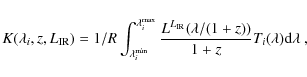 |
(A.3) |
where
As mentioned in the main text, from the point of view of the conditioning of the inverse problem, it is preferable to reformulate Eq. (A.1)
in terms of
![]() ,
,
![]() and
and
![]() :
:
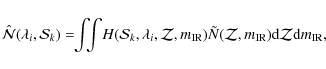
where the kernel of Eq. (A.4) reads
![\begin{displaymath}H(\mathcal{S},\lambda,\mathcal{Z},m_{\rm IR})\equiv 10^{2.5 \...
... D}\!\left[S-F(\lambda,10^\mathcal{Z},10^{m_{\rm IR}})\right]
\end{displaymath}](/articles/aa/full_html/2009/36/aa09945-08/img80.png)
with
 |
(A.5) |
 |
(A.6) |
Here we have introduced the Euclidian-normalized number count,
A.2 Discretization
Let us project
![]() onto a complete basis of
onto a complete basis of
![]() functions
functions
of finite (asymptotically zero) support, which are chosen here to be piecewise constant step functions:
The parameters to fit are the weights njl.
Calling
![]() (the
(the ![]() parameters) and
parameters) and
![]() (the
(the
![]() measurements), Eq. (A.4)
then becomes formally
measurements), Eq. (A.4)
then becomes formally
where M is a
A.3 Penalties
Assuming that the noise in
![]() can be
approximated to be Normal, we can estimate the error between the measured
counts and the non-parametric model by
can be
approximated to be Normal, we can estimate the error between the measured
counts and the non-parametric model by

where the weight matrix W is the inverse of the covariance matrix of the data (which is diagonal for uncorrelated noise with diagonal elements equal to one over the data variance). Since we are interested here in a non-parametric inversion, the decomposition in Eq. (A.7) typically involves many more parameters than constraints, such that each parameter controls the shape of the function,
where K is a positive definite matrix, which is chosen so that R in Eq. (A.10) should be non zero when X is strongly varying as a function of its indices. In practice, we use a square Laplacian penalization D2 norm as defined by Eq. (30) of Ocvirk et al. (2006b). Indeed, a Tikhonov penalization does not explicitly enforce smoothness of the solution, and a square gradient penalization favors flat solutions that are unphysical in our problem.
As mentioned in the main text, for a range of redshifts, a direct
measurement,
X0, which can be used as a prior for ![]() ,
is available. We may therefore
add as a supplementary constraint that
,
is available. We may therefore
add as a supplementary constraint that

should remain small, where the weight matrix, W2, is the inverse of the covariance matrix of the prior, X0, and should be non zero over the appropriate redshift range. In short, the penalized non-parametric solution of Eq. (A.8) accounting for both penalties is found by minimizing the so-called objective function
where L(X), R(X), and P(X) are the likelihood and regularization terms given by Eqs. (A.9)- (A.11), respectively. The Lagrange multipliers
The minimum of the objective function, Q(X), given by Eq. (A.12) reads formally as
This equation clearly shows that the solution tends towards X0when
Appendix B: Test of robustness
To quantify the confidence level of the inversion technique, we test its robustness. Starting from an arbitrary LF, we produce IR counts in the bands and flux ranges corresponding to the observations from this LF. Then, we add some random Gaussian noise to the simulated counts, using the real uncertainty on the observations as the
The comparison of the input and output LFs is shown in
Fig. B.1. The error on the absolute difference in
![]() is represented in
gray levels and contours. The difference is generally less than
0.4 dex (factor 2.5) in the range where the LF can be constrained from
the observed counts (range of the z-L plane encompassed by the
dashed lines). A noticeable exception is the very low-redshift range
(z<0.1), which corresponds to bright sources. For such large fluxes,
the considerable noise in the observed counts produces large errors on
the recovered LF. At high redshift, recall that the ultra-luminous
population of galaxies appears as rare and very bright objects, in a
flux range where the number counts are poorly known.
is represented in
gray levels and contours. The difference is generally less than
0.4 dex (factor 2.5) in the range where the LF can be constrained from
the observed counts (range of the z-L plane encompassed by the
dashed lines). A noticeable exception is the very low-redshift range
(z<0.1), which corresponds to bright sources. For such large fluxes,
the considerable noise in the observed counts produces large errors on
the recovered LF. At high redshift, recall that the ultra-luminous
population of galaxies appears as rare and very bright objects, in a
flux range where the number counts are poorly known.
![\begin{figure}
\par\includegraphics[width=9cm,clip]{09945f11.ps}
\end{figure}](/articles/aa/full_html/2009/36/aa09945-08/img106.png) |
Figure B.1:
Estimated robustness of the LF inversion used in
this paper. The relative
difference between the input LF and the recovered LF
(when a realistic noise is added to the corresponding input counts) is larger for
darker parts of the diagram. This difference is relatively small (<0.4 dex)
in the region
of the z-L space effectively constrained by observations: the dotted
and dashed lines correspond to the extreme fluxes considered at 24 |
| Open with DEXTER | |
Appendix C: Model predictions for Herschel
In Sect. 4, we have inverted the known IR counts to obtain constraints on the evolving total IR LF. We have seen that the LF obtained through this inversion is realistic and matches most of the recent observations (counts, CIRB, Mid-IR LF at low redshift). Then, in Sect. 5.2, we have shown how we can measure directly a part of this LF with a good confidence and that the LF resulting from the inversion is in good agreement with this solid measurement, validating the LF obtained by this empirical modeling approach. In this section, we use the median LF obtained from the inversions to predict some counts which should be observed with future observations in the FIR with Herschel or SCUBA2.
At the time of publication, several new facilities
are in preparation to observe the Universe in the far-IR to sub-mm
regimes. The differential counts (normalized to Euclidean) at
wavelengths ranging from 16 to 850 ![]() m, which we derived from the
inversion technique, are presented in Fig. C.3. The
separation of the contribution of local, intermediate, and distant
galaxies in different colors illustrates the expected trend that
larger wavelengths are sensitive to higher redshifts, hence the relative
complementarity of all IR wavelengths. There will be a bias towards
more luminous and distant objects with increasing wavelength,
illustrated here for the Herschel passbands (see
Fig. C.4), but this may be used to pre-select the most
distant candidates expected to be detected only at the largest
wavelengths. In the following, we discuss the predictions of the
inversion technique for those instruments, as well as their respective
confusion limits, which is the main limitation of far-IR extragalactic
surveys.
m, which we derived from the
inversion technique, are presented in Fig. C.3. The
separation of the contribution of local, intermediate, and distant
galaxies in different colors illustrates the expected trend that
larger wavelengths are sensitive to higher redshifts, hence the relative
complementarity of all IR wavelengths. There will be a bias towards
more luminous and distant objects with increasing wavelength,
illustrated here for the Herschel passbands (see
Fig. C.4), but this may be used to pre-select the most
distant candidates expected to be detected only at the largest
wavelengths. In the following, we discuss the predictions of the
inversion technique for those instruments, as well as their respective
confusion limits, which is the main limitation of far-IR extragalactic
surveys.
The ESA satellite Herschel is scheduled to be launched within the next
year, while the next-generation IR astronomical satellite of the
Japanese space agency, SPICA, is scheduled for 2010, with a
contribution by ESA under discussion, including a mid-IR imager named
SAFARI. Both telescopes share the same diameter of 3.5 m, but
the lower telescope temperature of SPICA, combined with projected
competitive sensitivities, will make it possible to reach confusion
around 70 ![]() m (where Herschel is limited by integration time). The
5
m (where Herschel is limited by integration time). The
5![]() -1hour limits of the instruments SAFARI onboard SPICA
(50
-1hour limits of the instruments SAFARI onboard SPICA
(50 ![]() Jy, 33-210
Jy, 33-210 ![]() m, dashed line), PACS (3mJy,
55-210
m, dashed line), PACS (3mJy,
55-210 ![]() m, light blue line) and SPIRE (2 mJy, 200-670
m, light blue line) and SPIRE (2 mJy, 200-670 ![]() m,
blue line) onboard Herschel are compared in Fig. C.1
to the confusion limits that we derive from the best-fit model of the
inversion, at all wavelengths between 30 and 850
m,
blue line) onboard Herschel are compared in Fig. C.1
to the confusion limits that we derive from the best-fit model of the
inversion, at all wavelengths between 30 and 850 ![]() m, assuming the
the confusion limit definition given below.
m, assuming the
the confusion limit definition given below.
![\begin{figure}
\par\includegraphics[width=9cm,clip]{09945f12.ps}
\end{figure}](/articles/aa/full_html/2009/36/aa09945-08/img107.png) |
Figure C.1:
Confusion limit for a 3.5 m telescope. The
5 |
| Open with DEXTER | |
The definition of the confusion limit is not trivial, in particular because it depends on the level of clustering of galaxies; the optimum way to define it would be to perform simulations to compute the photometric error as a function of flux density, and then decide that the confusion limit is e.g. the depth above which 68% of the detected sources are measured with a photometric accuracy better than 20%. In the following, we only consider a simpler approach that involves computing the two sources of confusion that were discussed in Dole et al. (2003):
- the photometric confusion noise: the noise produced by sources fainter than the detection threshold. The photometric criterion corresponds to the requirement that sources are detected with an S/N(photometric) > 5;
- the fraction of blended sources: a requirement for the quality of
the catalog of sources will be that less than N % of the sources
are closer than 0.8
 FWHM, i.e. close enough to not be
separated.
FWHM, i.e. close enough to not be
separated.
![\begin{figure}
\par\includegraphics[width=8.7cm,clip]{09945f13.ps}
\end{figure}](/articles/aa/full_html/2009/36/aa09945-08/img112.png) |
Figure C.2:
Detection limits for confusion limited surveys from 70 to
850 |
| Open with DEXTER | |
Table C.1: Fraction of the CIRB resolved by confusion-limited Herschel surveys.
We note that the confusion limit for a 3.5 m-class telescope, such as Herschel, is ten times more than the depth it can reach in one hour (5
![\begin{figure}
\par\includegraphics[width=16.5cm,clip]{09945f14.ps}
\end{figure}](/articles/aa/full_html/2009/36/aa09945-08/img115.png) |
Figure C.3:
Counts predicted from the inversion in the far-infrared and sub-mm (solid line). The counts are
decomposed in redshift bins (blue = z<0.5; green = 0.5<z<1.5;
orange = 1.5<z<2.5; red = z>2.5). The oblique dashed line corresponds to
the limit in statistics due to the smallness of a field like GOODS
North+South or 0.07 square degrees: less than 2 galaxies per
flux bin of width
|
| Open with DEXTER | |
![\begin{figure}
\par\includegraphics[width=16.6cm,clip]{09945f15.ps}
\end{figure}](/articles/aa/full_html/2009/36/aa09945-08/img116.png) |
Figure C.4:
Differential counts predicted from the non-parametric
inversion for future Herschel observations: PACS 100 |
| Open with DEXTER | |
For comparison, we also illustrated the ground-based capacity of
ARTEMIS built by CEA-Saclay which will operate at the ESO 12
m-telescope facility APEX (Atacama Pathfinder EXperiment) at 200, 350
and 450 ![]() m and SCUBA-2 that will operate at the 15 m telescope
JCMT at 450 and 850
m and SCUBA-2 that will operate at the 15 m telescope
JCMT at 450 and 850 ![]() m. To avoid confusion between all
instruments, we only show the average wavelength 400
m. To avoid confusion between all
instruments, we only show the average wavelength 400 ![]() m for a 12
m-class telescope and 850
m for a 12
m-class telescope and 850 ![]() m for a 15 m-class telescope
(Fig. C.1). Although the confusion limit in the
850
m for a 15 m-class telescope
(Fig. C.1). Although the confusion limit in the
850 ![]() m passband is ten times below that of Herschel at the
longest wavelengths, this band is not competitive with the
m passband is ten times below that of Herschel at the
longest wavelengths, this band is not competitive with the
![]() 400
400 ![]() m one, which should be priorities for ARTEMIS and
SCUBA-2 for the study of distant galaxies, or with the 70 and
100
m one, which should be priorities for ARTEMIS and
SCUBA-2 for the study of distant galaxies, or with the 70 and
100 ![]() m ones for a 3.5 m space experiment such as SPICA and
Herschel, for redshifts below
m ones for a 3.5 m space experiment such as SPICA and
Herschel, for redshifts below ![]() .
We also note that only in
these two passbands will the cosmic IR background be resolved with
these future experiments (see Table C.1), which suggests
that a larger telescope size should be considered for a future
experiment to observe the far IR Universe above 100
.
We also note that only in
these two passbands will the cosmic IR background be resolved with
these future experiments (see Table C.1), which suggests
that a larger telescope size should be considered for a future
experiment to observe the far IR Universe above 100 ![]() m and below
the wavelength domain of ALMA. We did not mention here ALMA since it
will not be affected by these confusion issue: due to its very
good spatial resolution, it will be limited to either small ultradeep
survey, hence missing rare objects or follow-ups of fields observed
with single dish instruments, e.g. ARTEMIS. Finally, the JWST that
will operate in the mid IR will be a very powerful instrument for probing
the faintest star-forming galaxies in the distant Universe, but
predictions are difficult to produce at the present stage since it has
already been found that extrapolations from the mid to far IR become less
robust already at
m and below
the wavelength domain of ALMA. We did not mention here ALMA since it
will not be affected by these confusion issue: due to its very
good spatial resolution, it will be limited to either small ultradeep
survey, hence missing rare objects or follow-ups of fields observed
with single dish instruments, e.g. ARTEMIS. Finally, the JWST that
will operate in the mid IR will be a very powerful instrument for probing
the faintest star-forming galaxies in the distant Universe, but
predictions are difficult to produce at the present stage since it has
already been found that extrapolations from the mid to far IR become less
robust already at ![]() (e.g. Papovich et al. 2007; Pope et al. 2008; Daddi et al. 2007b).
(e.g. Papovich et al. 2007; Pope et al. 2008; Daddi et al. 2007b).
Footnotes
- ... counts
- Appendices are only available in electronic from at http://www.aanda.org
- ...
ULIRGS
- We adopt the following notation in this paper:
``Normal'' galaxies have ;
;
``LIRGS'': ;
;
``ULIRGS'': ;
;
``HLIRGS'': .
.
- ... others
- This approach is at variance with the classical ``direct'' methods used for this purpose, in which luminosities of individual sources are derived from their measured redshifts and fluxes in a single mid-IR band.
- ... versatile
- It is worth noting that we can take (optionally and when available) the redshift information into account by using as priors the luminosity functions measured at low redshifts from direct methods. We will show in Sect. 4 that this knowledge of the luminosity-redshift distribution at low redshift (z<2) brings actually little new to our results.
- ... galaxies
- In this subsection presenting the formalism in the general case, an evolution of the SEDs is considered as possible.
- ...
following
- If the SEDs vary not only with
 but
also with z, we could call it the ``e+k+d'' matrix.
but
also with z, we could call it the ``e+k+d'' matrix.
- ... completeness
- We could also have used a more classical approach to characterize the uncertainties in the recovered LFs by computing the posterior variance covariance of the parameters away from the itterative nonlinear solution, and compared it to the corresponding initial prior (hence constructing the so called information matrix). These uncertainties naturally arise from the uncertainties on the observed counts through the error matrix W. Instead, we favor here Monte-Carlo simulations because they yield similar - if not more robust (since we span ranges of possible nonlinear solutions) - constraints on the recovered LF.
- ... redshift
- Technically, this supplementary prior involves
again penalizing the formal
 by adding an extra term that
measures the distance between the observed LF and the solution (this
corresponds to
by adding an extra term that
measures the distance between the observed LF and the solution (this
corresponds to  in Appendix A). The LFs that
are too different from the known low-redshift LF are therefore
strongly penalized, so excluded de facto.
in Appendix A). The LFs that
are too different from the known low-redshift LF are therefore
strongly penalized, so excluded de facto.
- ...
conversion)
- Note that Le Floc'h et al. (2005) errors bars are rather large because they partly reflect the uncertainties in the SEDs of galaxies. We checked that using another library of SEDs (e.g. the LDP03 library) produces differences in our LFs comparable to the error bars of Le Floc'h et al. (2005).
- ... inversion
- The datasets are independent, indeed. But strictly speaking, it is actually not the case for the SFRD measurements because the libraries of SEDs used for k-corrections are the same in both methods.
All Tables
Table C.1: Fraction of the CIRB resolved by confusion-limited Herschel surveys.
All Figures
| |
Figure 1:
Observed 15/16 |
| Open with DEXTER | |
| In the text | |
| |
Figure 2:
24 |
| Open with DEXTER | |
| In the text | |
| |
Figure 3:
Mid- and Far-IR counts obtained from the non-parametric inversion of the
observed counts. The data counts that are the basis of the
inversion are represented by the shaded blue zones (fitted values |
| Open with DEXTER | |
| In the text | |
| |
Figure 4:
All possible solutions for the evolving LFs that best reproduce
all the IR counts of Fig. 3 and the CIRB
constraints. As in Fig. 3, the thick red line and
the dashed red areas represent the best-fitting solution and the range of
allowed solutions, respectively. By construction, no conclusion on the
LF can be made in the vertical gray-shaded areas where a divergence is
expected because these objects are not seen in the counts because of the flux limits of
current IR surveys. At the top of each panel, the ranges of
|
| Open with DEXTER | |
| In the text | |
| |
Figure 5: Star-formation rate density since z=5 derived from the counts inversions. The SFRD is obtained from the range of all possible luminosity functions derived from the counts and respecting the CIRB constraints. The solid lines correspond to the best fit to the counts and the transparent shaded areas show the range of uncertainties. From top to bottom at z=0.8: black = all galaxies, green = LIRGS, blue = normal star-forming galaxies, orange = ULIRGS, red = HLIRGS. |
| Open with DEXTER | |
| In the text | |
| |
Figure 6:
Top and bottom left: counts at 16, 24, and 70 |
| Open with DEXTER | |
| In the text | |
| |
Figure 7:
Total IR luminosity functions derived independently
from the counts
inversion and from direct measurements. ``Clipped'' CE01 templates are used for the 24 |
| Open with DEXTER | |
| In the text | |
| |
Figure 8:
Total SFRD regions compared to ilation of direct
measurements from Hopkins & Beacom (2006) (empty circles and error bars
only for z>1.5 for clarity purposes). The outer light-gray regions
corresponds to all possible LFs fitting the counts. The inner darker
region includes 68% of these models. The dashed line corresponds to
the LF producing the best-fit to the multi- |
| Open with DEXTER | |
| In the text | |
| |
Figure 9: History of the SFRD decomposed in four infrared luminosity classes. The inversion results (full set of models and 68% inner region) are shown with gray-shaded areas. The total SFRD history (68% inner region) is also shown for reference in each panel as dotted lines. Our direct (and independent) measurements from the GOODS survey are shown as triangles. Empty triangles are used for bins affected by completeness. The z=3 point for HLIRGS is subject to caveats (see text for details) so is probably overestimated. |
| Open with DEXTER | |
| In the text | |
| |
Figure 10: Range of allowed evolutions of the stellar mass density computed with the range of cosmic SF histories of Fig. 5. The dashed lines corresponds to the best-fit to the IR counts. The data points with error bars are measurements from Pérez-González et al. (2008) (empty circles) and Elsner et al. (2008) (filled dots). The realistic Baldry & Glazebrook (2003) IMF is used both for the data points and to derive the stellar mass density from the SFR density. |
| Open with DEXTER | |
| In the text | |
| |
Figure B.1:
Estimated robustness of the LF inversion used in
this paper. The relative
difference between the input LF and the recovered LF
(when a realistic noise is added to the corresponding input counts) is larger for
darker parts of the diagram. This difference is relatively small (<0.4 dex)
in the region
of the z-L space effectively constrained by observations: the dotted
and dashed lines correspond to the extreme fluxes considered at 24 |
| Open with DEXTER | |
| In the text | |
| |
Figure C.1:
Confusion limit for a 3.5 m telescope. The
5 |
| Open with DEXTER | |
| In the text | |
| |
Figure C.2:
Detection limits for confusion limited surveys from 70 to
850 |
| Open with DEXTER | |
| In the text | |
| |
Figure C.3:
Counts predicted from the inversion in the far-infrared and sub-mm (solid line). The counts are
decomposed in redshift bins (blue = z<0.5; green = 0.5<z<1.5;
orange = 1.5<z<2.5; red = z>2.5). The oblique dashed line corresponds to
the limit in statistics due to the smallness of a field like GOODS
North+South or 0.07 square degrees: less than 2 galaxies per
flux bin of width
|
| Open with DEXTER | |
| In the text | |
| |
Figure C.4:
Differential counts predicted from the non-parametric
inversion for future Herschel observations: PACS 100 |
| Open with DEXTER | |
| In the text | |
Copyright ESO 2009
Current usage metrics show cumulative count of Article Views (full-text article views including HTML views, PDF and ePub downloads, according to the available data) and Abstracts Views on Vision4Press platform.
Data correspond to usage on the plateform after 2015. The current usage metrics is available 48-96 hours after online publication and is updated daily on week days.
Initial download of the metrics may take a while.