| Issue |
A&A
Volume 504, Number 1, September II 2009
|
|
|---|---|---|
| Page(s) | 15 - 32 | |
| Section | Cosmology (including clusters of galaxies) | |
| DOI | https://doi.org/10.1051/0004-6361/200911811 | |
| Published online | 09 July 2009 | |
The simulated H I sky at low redshift
A. Popping1,2 - R. Davé3 - R. Braun2 - B. D. Oppenheimer3
1 - Kapteyn Astronomical Institute, PO Box 800, 9700 AV Groningen, The Netherlands
2 -
Australia Telescope National Facility, CSIRO, PO Box 76, Epping, NSW 1710, Australia
3 -
Astronomy Department, University of Arizona, Tucson, AZ 85721, USA
Received 8 February 2009 / Accepted 15 June 2009
Abstract
Context. Observations of intergalactic neutral hydrogen can provide a wealth of information about structure and galaxy formation, potentially tracing accretion and feedback processes on Mpc scales. Below a column density of
![]() cm-2, the ``edge'' or typical observational limit for H I emission from galaxies, simulations predict a cosmic web of extended emission and filamentary structures. Current observations of this regime are limited by telescope sensitivity, which will soon advance substantially.
cm-2, the ``edge'' or typical observational limit for H I emission from galaxies, simulations predict a cosmic web of extended emission and filamentary structures. Current observations of this regime are limited by telescope sensitivity, which will soon advance substantially.
Aims. We study the distribution of neutral hydrogen and its 21-cm emission properties in a cosmological hydrodynamic simulation, to gain more insight into the distribution of H I below
![]() cm-2. Such Lyman limit systems are expected to trace out the cosmic web and are relatively unexplored.
cm-2. Such Lyman limit systems are expected to trace out the cosmic web and are relatively unexplored.
Methods. Beginning with a 32 h-1 Mpc simulation, we extract the neutral hydrogen component by determining the neutral fraction, including a post-processed correction for self-shielding based on the thermal pressure. We take molecular hydrogen into account, assuming an average density ratio
![]() at z = 0. The statistical properties of the H I emission are compared with observations, to assess the reliability of the simulation. We then make predictions for upcoming surveys.
at z = 0. The statistical properties of the H I emission are compared with observations, to assess the reliability of the simulation. We then make predictions for upcoming surveys.
Results. The simulated H I distribution robustly describes the full column density range between
![]() and
and
![]() cm-2 and agrees very well with available measurements from observations. Furthermore there is good correspondence in the statistics when looking at the two-point correlation function and the H I mass function. The reconstructed maps are used to simulate observations of existing and future telescopes by adding noise and accounting for the sensitivity of the telescopes.
cm-2 and agrees very well with available measurements from observations. Furthermore there is good correspondence in the statistics when looking at the two-point correlation function and the H I mass function. The reconstructed maps are used to simulate observations of existing and future telescopes by adding noise and accounting for the sensitivity of the telescopes.
Conclusions. The general agreement in statistical properties of H I suggests that neutral hydrogen, as modelled in this hydrodynamic simulation, is a fair representation of neutral hydrogen in the Universe. Our method can be applied to other simulations, to compare different models of accretion and feedback. Future H I observations will be able to probe the regions where galaxies connect to the cosmic web.
Key words: intergalactic medium - cosmology: miscellaneous - galaxies: structure
1 Introduction
Current cosmological models ascribe only about 4% of the density in
the Universe to baryons (Spergel et al. 2007). The majority of
these baryons reside outside of galaxies, with stars and cold galactic
gas possibly accounting for about about one third
(Fukugita et al. 1998). Intergalactic baryons have historically
been traced in absorption, such as the Ly![]() forest arising from
diffuse photo-ionised gas that may account for up to 30% of baryons.
The remaining baryons are predicted to exist in a warm-hot
intergalactic medium (WHIM)
(e.g. Cen & Ostriker 1999; Davé et al. 1999,2001), which is shock-heated during the collapse of
density perturbations that give rise to the cosmic web. Nonetheless,
absorption probes yield only one-dimensional redshift-space
information, or in rare cases several probes through common
structures. Mapping intergalactic baryons in emission can in
principle provide morphological and kinematic information on accreting
(and perhaps out-flowing) gas within the cosmic web.
forest arising from
diffuse photo-ionised gas that may account for up to 30% of baryons.
The remaining baryons are predicted to exist in a warm-hot
intergalactic medium (WHIM)
(e.g. Cen & Ostriker 1999; Davé et al. 1999,2001), which is shock-heated during the collapse of
density perturbations that give rise to the cosmic web. Nonetheless,
absorption probes yield only one-dimensional redshift-space
information, or in rare cases several probes through common
structures. Mapping intergalactic baryons in emission can in
principle provide morphological and kinematic information on accreting
(and perhaps out-flowing) gas within the cosmic web.
Unfortunately, emission from intergalactic baryons is difficult to
observe, because current telescope sensitivities result in a detection
limit of column densities
![]() cm-2, which
are the realm of damped Ly
cm-2, which
are the realm of damped Ly![]() (DLA) systems and sub-DLAs. Below
column densities of
(DLA) systems and sub-DLAs. Below
column densities of ![]()
![]() cm-2, the
neutral fraction of hydrogen decreases rapidly because of the transition
from optically-thick to optically-thin gas ionised by the metagalactic
ultraviolet flux. At lower densities, the gas is no longer affected by
self-shielding and the atoms are mostly ionised. This sharp decline
in neutral fraction from almost unity to less than a percent happens
within a few kpc (Dove & Shull 1994). Below
cm-2, the
neutral fraction of hydrogen decreases rapidly because of the transition
from optically-thick to optically-thin gas ionised by the metagalactic
ultraviolet flux. At lower densities, the gas is no longer affected by
self-shielding and the atoms are mostly ionised. This sharp decline
in neutral fraction from almost unity to less than a percent happens
within a few kpc (Dove & Shull 1994). Below
![]() cm-2, the gas is optically thin and the decline in
neutral fraction with total column is much more gradual. A consequence
of this rapid decline in neutral fraction is a plateau in the
H I column density distribution function between
cm-2, the gas is optically thin and the decline in
neutral fraction with total column is much more gradual. A consequence
of this rapid decline in neutral fraction is a plateau in the
H I column density distribution function between
![]() and
and
![]() cm-2, where the relative surface area at these columns shows only
modest growth. This behaviour is confirmed in QSO absorption studies
tabulated by Corbelli & Bandiera (2002) and in H I
emission by Braun & Thilker (2004). Below
cm-2, where the relative surface area at these columns shows only
modest growth. This behaviour is confirmed in QSO absorption studies
tabulated by Corbelli & Bandiera (2002) and in H I
emission by Braun & Thilker (2004). Below
![]() cm-2 the relative surface area increases rapidly,
reaching about a factor of 30 larger at
cm-2 the relative surface area increases rapidly,
reaching about a factor of 30 larger at
![]() compared with
compared with
![]() cm-2.
cm-2.
This plateau in the distribution function is a critical issue for
observers of neutral hydrogen in emission. Although telescope
sensitivities have increased substantially over the past decades,
the detected surface area of galaxies observed in the 21-cm line has
only increased modestly (eg. Dove & Shull 1994). Clearly
there is a flattening in the distribution function near
![]() cm-2 which has limited the ability of even deep
observations to detect hydrogen emission from a larger area. By
establishing that a steeper distribution function is again expected below
about
cm-2 which has limited the ability of even deep
observations to detect hydrogen emission from a larger area. By
establishing that a steeper distribution function is again expected below
about
![]() ,
it provides a clear technical
target for what the next generation of radio telescopes needs to
achieve to effectively probe diffuse gas.
,
it provides a clear technical
target for what the next generation of radio telescopes needs to
achieve to effectively probe diffuse gas.
Exploration of the
![]() cm-2 regime is
essential for gaining a deeper understanding of the repository of
baryons that drive galaxy formation and evolution. This gas, residing
in filamentary structures, is the reservoir that fuels future star
formation, and could provide a direct signature of smooth cold-mode
accretion predicted to dominate gas acquisition in star-forming
galaxies today (Dekel et al. 2009; Keres et al. 2005,2009). Furthermore, the trace neutral fraction in this
phase may provide a long-lived fossil record of tidal interactions and
feedback processes such as galactic winds and AGN-driven cavities.
cm-2 regime is
essential for gaining a deeper understanding of the repository of
baryons that drive galaxy formation and evolution. This gas, residing
in filamentary structures, is the reservoir that fuels future star
formation, and could provide a direct signature of smooth cold-mode
accretion predicted to dominate gas acquisition in star-forming
galaxies today (Dekel et al. 2009; Keres et al. 2005,2009). Furthermore, the trace neutral fraction in this
phase may provide a long-lived fossil record of tidal interactions and
feedback processes such as galactic winds and AGN-driven cavities.
Several new large facilities to study 21cm emission are under development today. In view of the observational difficulties in probing the low H I column regime, it is particularly important to have reliable numerical simulations to aid in planning new observational campaigns, and eventually to help interpret such observations within a structure formation context. While simulations of galaxy formation are challenging, historically they have had much success predicting the more diffuse baryons residing in the cosmic web (e.g. Davé et al. 1999). If such simulations display statistical agreement with key existing H I emission data, then they can be used to make plausible predictions for the types of structures that may be detected, along with suggesting optimum observing strategies.
In this paper, we employ a state-of-the art cosmological hydrodynamic
simulation to study H I emission from filamentary
large-scale structure and the galaxies within them. The simulation
used here include a well-constrained prescription for galactic
outflows that has been shown to reproduce the observed metal and
H I absorption line properties from
![]() (Oppenheimer & Davé 2008,2006,2009). We develop a method to
produce H I maps from these simulations, and compare
statistical properties of the reconstructed H I data
with the statistics of real H I observations, to
assess the reliability of the simulation. For this purpose we will
primarily use the H I Parkes All Sky Survey (HIPASS)
(Barnes et al. 2001) since this is the largest available
H I survey. This work is intended to provide an
initial step towards a more thorough exploration of model constraints
that will be enabled by comparisons with present and future
H I data.
(Oppenheimer & Davé 2008,2006,2009). We develop a method to
produce H I maps from these simulations, and compare
statistical properties of the reconstructed H I data
with the statistics of real H I observations, to
assess the reliability of the simulation. For this purpose we will
primarily use the H I Parkes All Sky Survey (HIPASS)
(Barnes et al. 2001) since this is the largest available
H I survey. This work is intended to provide an
initial step towards a more thorough exploration of model constraints
that will be enabled by comparisons with present and future
H I data.
Note that current spatial resolution of simulations having cosmologically-representative volumes cannot reproduce a galaxy as would be seen with H I observations having sub-kpc resolution. Therefore we do not consider the internal kinematics or detailed shapes of the objects associated with simulated galaxies. We can only assess the statistical properties of the diffuse H I phase and predict how the gas is distributed on multi-kpc scales. We particularly focus on lower column density material that may be probed with future H I surveys, which primarily reside in cosmic filaments within which galaxies are embedded.
Our paper is organised as follows. In section two we briefly describe the particular simulation that has been analysed. In section three we describe our method to extract the neutral hydrogen from the simulations. The neutral fraction is determined from both a general ionisation balance as well as a local self-shielding correction. We also model the transition from atomic to molecular hydrogen We present our results, showing the statistical properties of the recovered H I in section four, where they are compared with similar statistics obtained from observations. The distribution of neutral hydrogen is compared with the distribution of dark matter and stars in this section as well. In the fifth section we discuss the results and outline the implications. Finally, section six reiterates our main conclusions.
2 Simulation code
A modified version of the N-body+hydrodynamic code Gadget-2 is employed, which uses a tree-particle-mesh algorithm to compute gravitational forces on a set of particles, and an entropy-conserving formulation of smoothed particle hydrodynamics (SPH: Springel & Hernquist 2002) to simulate pressure forces and shocks in the baryonic gaseous particles. This Lagrangian code is fully adaptive in space and time, allowing simulations with a large dynamic range necessary to study both high-density regions harbouring galaxies and the lower-density IGM. It includes a prescription for star formation following Springel & Hernquist (2003b) and galactic outflows as described below. The code has been described in detail in Oppenheimer & Davé (2006, 2008); we will only summarise the properties here.
The novel feature of our simulation is that it includes a
well-constrained model for galactic outflows. The implementation
follows Springel & Hernquist (2003a), but employs scaling of outflow
speed and mass loading factor with galaxy mass as expected for
momentum-driven winds (Murray et al. 2005). Our simulations
using these scalings have been shown to successfully reproduce a wide
range of IGM and galaxy data, including IGM enrichment as traced by
![]() -6 C IV absorbers (Oppenheimer & Davé 2006), the
galaxy mass-metallicity relation (Finlator & Davé 2008), the
early galaxy luminosity function and its
evolution (Davé et al. 2006), O VI absorption at
low-z (Oppenheimer & Davé 2009), and enrichment and entropy
levels in galaxy groups (Davé et al. 2008). Such outflows
are expected to impact the distribution of gas in the large-scale
structure around galaxies out to typically
-6 C IV absorbers (Oppenheimer & Davé 2006), the
galaxy mass-metallicity relation (Finlator & Davé 2008), the
early galaxy luminosity function and its
evolution (Davé et al. 2006), O VI absorption at
low-z (Oppenheimer & Davé 2009), and enrichment and entropy
levels in galaxy groups (Davé et al. 2008). Such outflows
are expected to impact the distribution of gas in the large-scale
structure around galaxies out to typically ![]() 100 kpc
(Oppenheimer & Davé 2008,2009), so are
important for studying the regions expected to yield detectable
H I emission.
100 kpc
(Oppenheimer & Davé 2008,2009), so are
important for studying the regions expected to yield detectable
H I emission.
The simulation used here is run with cosmological parameters
consistent with the 3-year WMAP results (Spergel et al. 2007).
The parameters are
![]() ,
,
![]() ,
,
![]() ,
H0 = 71 km s-1 Mpc-1,
,
H0 = 71 km s-1 Mpc-1,
![]() ,
and n
= 0.95. The periodic cubic volume has a box length of 32 h-1 Mpc
(comoving), and the gravitational softening length is set to 2.5 h-1kpc (comoving). Dark matter and gas are represented using 2563particles each, yielding a mass per dark matter and gas particle of
,
and n
= 0.95. The periodic cubic volume has a box length of 32 h-1 Mpc
(comoving), and the gravitational softening length is set to 2.5 h-1kpc (comoving). Dark matter and gas are represented using 2563particles each, yielding a mass per dark matter and gas particle of
![]() and
and
![]() ,
respectively.
The simulation was started in the linear regime at z=129, with initial
conditions established using a random realisation of the power spectrum
computed following Eisenstein & Hu (1999), and evolved to z=0.
,
respectively.
The simulation was started in the linear regime at z=129, with initial
conditions established using a random realisation of the power spectrum
computed following Eisenstein & Hu (1999), and evolved to z=0.
3 Method for making H I maps
We now describe the algorithm used to extract the neutral hydrogen
component from this simulation. The method developed is general, and
can be applied to any simulation that has a similar set of output
parameters. In our analysis, we set the total hydrogen number density
to
![]() where
where
![]() is the mass
of the hydrogen atom. The factor 0.74 assumes a helium abundance of Y
= 0.26 by mass, and that all the helium is in the form of
He I and He II with a similar neutral
fraction as hydrogen. Apart from this factor the presence of helium is
not taken into account in our calculations. We will describe how we
determine the neutral fraction of the gas particles, including
applying a correction for self shielding in high density regions and
taking into account molecular hydrogen formation where relevant. This
allows reconstruction of the neutral hydrogen distribution, by mapping
the particles onto a three dimensional grid.
is the mass
of the hydrogen atom. The factor 0.74 assumes a helium abundance of Y
= 0.26 by mass, and that all the helium is in the form of
He I and He II with a similar neutral
fraction as hydrogen. Apart from this factor the presence of helium is
not taken into account in our calculations. We will describe how we
determine the neutral fraction of the gas particles, including
applying a correction for self shielding in high density regions and
taking into account molecular hydrogen formation where relevant. This
allows reconstruction of the neutral hydrogen distribution, by mapping
the particles onto a three dimensional grid.
3.1 Neutral fraction of hydrogen
We begin by calculating the neutral fraction from the density and temperature of gas in the simulations, together with the H I photo-ionisation rate provided by the cosmic UV background. Dove & Shull (1994) found that the radial structure of the column density of H I is more sensitive to the extra-galactic radiation field than to the distribution of mass in the host galaxy. When calculating the neutral fraction, we assume that all photo-ionisation is due to radiation external to the disk and that internal stellar sources are not significant. In this case the nebular model as described in Osterbrock (1989) is a very good approximation, since the typical number density in the outer parts of galaxies, approximately 10-2cm-3, is so low that collisional ionisation is negligible. When going further out, the densities become even lower. Inside galaxies the volume densities are so high, that the neutral fraction is of order unity owing to self-shielding.
In the IGM, hydrogen becomes ionised when the extreme ultraviolet (UV)
radiation ionises and heats the surrounding gas. On the other hand,
the recombination of electrons leads to neutralisation. The degree of
ionisation is determined by the balance between photo-ionisation and
radiative recombination. Only photons more energetic than
![]() eV can ionise hydrogen. The ionisation equilibrium equation is given by e.g. Osterbrock (1989) as:
eV can ionise hydrogen. The ionisation equilibrium equation is given by e.g. Osterbrock (1989) as:
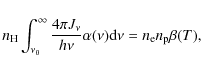 |
(1) |
where
| (2) |
where
| (3) |
with n the total density.
We can write the ionisation balance for neutral hydrogen as
 |
(4) |
where
With this equation it is easy to determine the neutral fraction, which is given by
 |
(5) |
using
 |
(6) |
Obviously the neutral fractions that we calculate are closely related to the values we use for the photo-ionisation and recombination rate. The photo-ionisation rate at low redshift is not well constrained observationally; by combining Ly
The recombination rate coefficients are dependent on temperature.
We make use of an analytic function described by
Verner & Ferland (1996), that fits the coefficients in the
temperature range form 3 K to 1010 K:
![\begin{displaymath}\beta(T) = a \Big[
\sqrt{T/T_0}\big(1+\sqrt{T/T_0}\big)^{1-b}\big(1+\sqrt{T/T_1}\big)^{1+b}
\Big] ^{-1}
\end{displaymath}](/articles/aa/full_html/2009/34/aa11811-09/img56.png) |
(7) |
where a, b, T0 and T1 are the fitting parameters. For the H I ion the fitting parameters are:
The neutral fraction is plotted for different temperatures as function of density of H atoms in Fig. 1. For temperatures below 104 K, the neutral fraction is still significant (a few percent) at reasonably low densities of 0.01 cm-3 but at higher temperatures most of the gas is ionised, and the neutral fraction drops very quickly.
![\begin{figure}
\par\includegraphics[width=8.4cm,clip]{11811f01.eps}
\end{figure}](/articles/aa/full_html/2009/34/aa11811-09/img59.png) |
Figure 1: Neutral fraction as a function of density for different temperatures between 104 and 109 K. |
| Open with DEXTER | |
3.2 Molecular hydrogen
When gas has cooled sufficiently, it coexists in the
molecular (H2) and atomic (H I) phases. The
H2 regions are found in dense molecular clouds where star
formation occurs. Unfortunately there is large uncertainty in the
average amount of H2 in galaxies, as estimates have to rely on indirect
tracers and conversion factors, for which the dependancies are not
well-understood. As a result, there is substantial variance in
estimates of the average density ratio at z=0,
![]() (e.g. 0.42 and 0.26 stated
respectively by Keres et al. 2003 and
Obreschkow & Rawlings 2009). It is beyond the scope of this paper to
revisit these determinations, therefore we will adopt a value of
(e.g. 0.42 and 0.26 stated
respectively by Keres et al. 2003 and
Obreschkow & Rawlings 2009). It is beyond the scope of this paper to
revisit these determinations, therefore we will adopt a value of
![]() that falls within the error bars
of current estimates. Given the observed local value of the atomic
mass density, of
that falls within the error bars
of current estimates. Given the observed local value of the atomic
mass density, of
![]() Mpc-3 (Zwaan et al. 2003), this implies a molecular
mass density of
Mpc-3 (Zwaan et al. 2003), this implies a molecular
mass density of
![]() Mpc-3.
Mpc-3.
To define the regions of molecular hydrogen, we use a threshold based on the thermal pressure (P/k = nT). Wong & Blitz (2002), Blitz & Rosolowsky (2004) and more recently Blitz & Rosolowsky (2006) have made the case that the amount of molecular hydrogen that is formed in galaxies is determined by only one parameter, the interstellar gas pressure. In hydrostatic pressure equilibrium, the hydrostatic pressure is balanced by the sum of all contributions to the gas pressure: magnetic pressure, cosmic ray pressure and kinetic pressure terms (of which the thermal pressure is relatively small) (e.g. Walterbos & Braun 1996, and references therein). However, thermal pressure is directly coupled to energy dissipation via radiation, and therefore thermal pressure can track the total pressure due to various equipartition mechanisms. An evaluation of the various contributions to the total hydrostatic pressure is given by Boulares & Cox (1990).
![\begin{figure}
\par\includegraphics[width=8.4cm,clip]{11811f02.eps}
\end{figure}](/articles/aa/full_html/2009/34/aa11811-09/img63.png) |
Figure 2: Temperatures are plotted against densities for every 200 th. particle in the simulation. The dashed (blue) and dash-dotted (red) lines correspond to constant thermal pressures of P/k = 155 and 810 cm-3 K, that were found empirically to reproduce the observed mass densities of atomic and molecular gas at z = 0. The solid (green) line shows where the recombination time is equal to the sound-crossing time at a physical scale of one kpc. Particles above/left of the green line are unlikely to be neutral or molecular. |
| Open with DEXTER | |
Two lines of constant thermal pressure are shown in Fig. 2 where temperatures are plotted against density for individual particles in the simulation. When following these lines, they cross two regions, one with high densities and low temperatures and one with moderate densities, but very high temperatures. These two regions are distinguished by the solid green line in Fig. 2, where the radiative recombination time is equivalent to the sound-crossing time on a kilo-parsec scale. The radiative recombination time is given in Tielens (2005) by:
 |
(8) |
where
For each particle the thermal pressure can be calculated and particles
with a pressure exceeding the threshold value and satisfying
![]() are considered molecular. By
exploring different pressure values as shown in Fig. 3, the
threshold can be tuned to yield the required molecular mass density,
are considered molecular. By
exploring different pressure values as shown in Fig. 3, the
threshold can be tuned to yield the required molecular mass density,
![]() Mpc-3. The
threshold thermal pressure value we empirically determine is P/k =
810 cm-3 K. We must stress, that this value is very likely not
a real physical value, as the resolution in our simulation is not
sufficient to resolve the scales of molecular clouds. Molecular clouds
have smaller scales with higher densities, which will likely have
significantly enhanced pressures.
Mpc-3. The
threshold thermal pressure value we empirically determine is P/k =
810 cm-3 K. We must stress, that this value is very likely not
a real physical value, as the resolution in our simulation is not
sufficient to resolve the scales of molecular clouds. Molecular clouds
have smaller scales with higher densities, which will likely have
significantly enhanced pressures.
![\begin{figure}
\par\includegraphics[width=8.4cm,clip]{11811f03.eps} \end{figure}](/articles/aa/full_html/2009/34/aa11811-09/img68.png) |
Figure 3:
The average molecular density at z = 0 is plotted
against the threshold thermal pressure, where molecular hydrogen
is assumed to form from atomic, while also satisfying the
condition that
|
| Open with DEXTER | |
3.3 Correction for self-shielding
Although the ionisation state and kinetic temperature are determined self-consistently within the simulation, it has been necessary to assume that each gas particle is subjected to the same all-pervasive radiation field. At both extremely low and high particle densities this approximation is sufficient, since local conditions will dominate. However, at intermediate densities, the ``self-shielding'' of particles by their neighbours may play a critical role in permitting local recombination, when the same particle would be substantially ionised in isolation. Present cosmological simulations are not capable of solving the full radiative transfer equations, although it is now becoming possible to post-process radiative transfer on individual galaxies (e.g. Pontzen et al. 2008). Because we want to study emission from the IGM as well as galaxies, we must instead adopt a simple correction based on density and temperature to approximate self-shielding. We adopt a similar approach to the one that was used to model the atomic to molecular transition above, using the thermal pressure as a proxy for the hydrostatic pressure. Only gas at a sufficiently high thermal pressure and for which the recombination time is shorter than the sound crossing time on kpc scales is assumed to recombine. Particles that satisfy the pressure and time-scale condition are considered to be fully self-shielded, and their neutral fraction is set to unity.
We will assume that the highest pressure regions which satisfy
![]() have already provided
have already provided
![]() Mpc-3 as discussed
above. We subsequently calculate the atomic density as
function of the thermal pressure
threshold, as shown in Fig. 4. It is empirically found,
that a threshold value of P/k = 155 cm-3 K results in an
H I density of
Mpc-3 as discussed
above. We subsequently calculate the atomic density as
function of the thermal pressure
threshold, as shown in Fig. 4. It is empirically found,
that a threshold value of P/k = 155 cm-3 K results in an
H I density of
![]() Mpc-3, that is similar to the derived value in
Zwaan et al. (2003). We will adopt this threshold value for our
further analysis.
Mpc-3, that is similar to the derived value in
Zwaan et al. (2003). We will adopt this threshold value for our
further analysis.
The typical densities and temperatures where self-shielding becomes
important are not accurately defined. When looking at Fig. 2,
the typical temperatures and densities which satisfy our empirical thermal
pressure criterion for local recombination are temperatures of ![]() 104 K and densities of
104 K and densities of ![]() 0.01 cm-3. These values agree well with
various estimates from literature
(e.g. Weinberg et al. 1997; Wolfire et al. 2003;
Pelupessy 2005).
0.01 cm-3. These values agree well with
various estimates from literature
(e.g. Weinberg et al. 1997; Wolfire et al. 2003;
Pelupessy 2005).
![\begin{figure}
\par\includegraphics[width=8.2cm,clip]{11811f04.eps} \end{figure}](/articles/aa/full_html/2009/34/aa11811-09/img72.png) |
Figure 4:
The average H I mass density at
z = 0 is plotted against the threshold thermal pressure, where
atomic hydrogen is assumed to recombine from ionised, while also
satisfying the condition that
|
| Open with DEXTER | |
3.4 Gridding method
To reconstruct the density fields, we have employed a grid-based method,
in which the value of the density field is calculated at a set of
locations defined on a regular grid. The mass of each particle is
spread over this grid in accordance with a particular weighting
function W, to yield
 |
(9) |
where
We adopt the weighting function directly from what is used for SPH in
Gadget-2, namely a spline kernel defined by Monaghan & Lattanzio (1985):
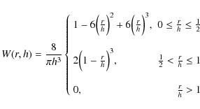 |
(10) |
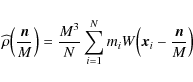
where r is the distance from the position of a particle and h is the smoothing length for each particle (which in Gadget-2 is the radius that encloses 32 gas particle masses). Furthermore we set a limit to the size of the smoothing length: the smoothing length of a particle has to be at least 1.5 times the resolution of the grid-cells, which means that a particle is distributed over at least three grid-cells in each dimension. This adversely affects the highest density regions in the reconstructed field (when insufficient gridding resolution is employed), but gives a more realistic representation of resolved objects and transitions without shot noise or step functions. We note that our procedure explicitly conserves total mass.
4 Results
Reconstructed density fields are gridded in three dimensions, for
the total hydrogen component (ionised plus neutral) the neutral
component and the molecular component. This makes it possible to
compare the distribution of the total and neutral hydrogen budget and
permits determination of neutral fractions for the volume and column
densities. Initially the full 32 h-1 Mpc cubes is gridded with a
cell size of 80 kpc. This allows visualisation of the distribution on
large scales and determination of the average density of neutral
hydrogen in the simulation volume
![]() .
The degree
of clustering can be determined by looking at the two-point
correlation function. However, this low resolution grid is not
suitable to resolve the high density regions and small structures, as
we will describe later. High density regions of the simulation volume
were selected and gridded with a cell-size of 2 kpc. The
H I column density distribution function and the
H I mass function can be determined from these regions. The
properties of the simulated H I gas will be
described and the statistics will be compared with the statistical
properties of observational data, mostly from the H
I Parkes All Sky Survey (HIPASS) (Barnes et al. 2001).
.
The degree
of clustering can be determined by looking at the two-point
correlation function. However, this low resolution grid is not
suitable to resolve the high density regions and small structures, as
we will describe later. High density regions of the simulation volume
were selected and gridded with a cell-size of 2 kpc. The
H I column density distribution function and the
H I mass function can be determined from these regions. The
properties of the simulated H I gas will be
described and the statistics will be compared with the statistical
properties of observational data, mostly from the H
I Parkes All Sky Survey (HIPASS) (Barnes et al. 2001).
Apart from gas or SPH particles, the simulations contain star and dark matter particles as well. We will adopt a relatively simple gridding scheme to reconstruct the distribution of stars and dark matter. This can be very useful to verify whether the stars, but especially the gas (or reconstructed H I) trace the distribution of Dark Matter.
![\begin{figure}
\par\mbox{\includegraphics[width=7.2cm,clip]{11811f05.eps} \includegraphics[width=7.2cm,clip]{11811f06.eps} }
\end{figure}](/articles/aa/full_html/2009/34/aa11811-09/img77.png) |
Figure 5: Left panel: H I distribution function after gridding to 80 kpc (dashed (red) line). The solid (blue) line corresponds to data gridded to a 2 kpc cell size. Filled dots correspond to the QSO absorption line data (Corbelli & Bandiera 2002). Right panel: combined H I distribution functions of the simulation, gridded to a resolution of 2 kpc (solid (blue) line) and 80 kpc (dashed (purple) line). Overlaid are distribution function from observational data of M 31 (Braun & Thilker 2004), WHISP (Swaters et al. 2002; Zwaan et al. 2005) and QSO absorption lines (Corbelli & Bandiera 2002) respectively. The reconstructed H I distribution function corresponds very well to all observed distribution functions. |
| Open with DEXTER | |
4.1 Mean H I density
The average H I density is an important
property, as this single number gives the amount of neutral hydrogen
that is reconstructed without any further analysis. The
H I density is very well determined from the 1000 brightest
HIPASS galaxies in Zwaan et al. (2003) They deduce an
H I density due to galaxies in the local universe of
![]() Mpc-3or
Mpc-3or
![]() Mpc-3 when taking into account biases like selection bias,
Eddington effect, H I self absorption and cosmic
variance. From Rosenberg & Schneider (2002) a value of
Mpc-3 when taking into account biases like selection bias,
Eddington effect, H I self absorption and cosmic
variance. From Rosenberg & Schneider (2002) a value of
![]() Mpc-3 can be
derived for the average H I density in the
universe. We will adopt the value of
Mpc-3 can be
derived for the average H I density in the
universe. We will adopt the value of
![]() Mpc-3.
The pressure thresholds for molecular and atomic hydrogen are tuned to
reproduce this density as is described earlier in this paper.
Mpc-3.
The pressure thresholds for molecular and atomic hydrogen are tuned to
reproduce this density as is described earlier in this paper.
4.2 H I distribution function
As mentioned above, the low and intermediate column densities
![]() cm-2) do not have a very significant
contribution to the total mass budget of H I.
cm-2) do not have a very significant
contribution to the total mass budget of H I.
For comparison with our simulation, the H I
distribution function derived from QSO absorption line data will be
used as tabulated in Corbelli & Bandiera (2002). For the QSO data the
column density distribution function
![]() is defined such
that
is defined such
that
![]() is the number of absorbers with
column density between
is the number of absorbers with
column density between
![]() and
and
![]() over an absorption distance interval
over an absorption distance interval ![]() .
We derive
.
We derive
![]() from the statistics of our reconstructed H I
emission. The column density distribution function in a reconstructed
cube can be calculated from,
from the statistics of our reconstructed H I
emission. The column density distribution function in a reconstructed
cube can be calculated from,
 |
(11) |
where
As the simulations contain H I column densities over
the full range between
![]() and 1021 cm-2, we can plot the H I column density
distribution function
and 1021 cm-2, we can plot the H I column density
distribution function
![]() over this entire range with
excellent statistics, in contrast to what has been achieved
observationally. In the left panel of Fig. 5 we overlay the
H I distribution functions we derive from the
simulations with the data values obtained from QSO absorption lines as
tabulated by Corbelli & Bandiera (2002) (black dots). The horizontal
lines on the QSO data points correspond to the bin-size over which
each data point has been derived. Vertical error bars are not shown,
as these have the same size as the dot. Around
over this entire range with
excellent statistics, in contrast to what has been achieved
observationally. In the left panel of Fig. 5 we overlay the
H I distribution functions we derive from the
simulations with the data values obtained from QSO absorption lines as
tabulated by Corbelli & Bandiera (2002) (black dots). The horizontal
lines on the QSO data points correspond to the bin-size over which
each data point has been derived. Vertical error bars are not shown,
as these have the same size as the dot. Around
![]() cm-2 there is only one data bin covering two orders of
magnitude in column density, illustrating the difficulty of sampling
this region with observations. This corresponds to the transition
between optically thick and thin gas, where only a small increase in
surface covering is associated with a large decrease in the column
density.
cm-2 there is only one data bin covering two orders of
magnitude in column density, illustrating the difficulty of sampling
this region with observations. This corresponds to the transition
between optically thick and thin gas, where only a small increase in
surface covering is associated with a large decrease in the column
density.
The dashed (red) line corresponds to data gridded to a 80 kpc cell size.
At low column densities the simulated distribution function agrees
very well with the QSO absorption line data. The transition from
optically thick to optically thin gas happens within just a few kpc of
radius in a galaxy disk (Dove & Shull 1994). Clearly a
reconstructed cube with a 80 kpc cell size does not have enough
resolution to resolve such transitions. Some form of plateau can be
recognised in the coarsely gridded data above
![]() cm-2, however it is not a smooth transition. Furthermore because
of the large cell size, no high column density regions can be
reconstructed at all. The cores of galaxies have high column
densities, but these are severely diluted within the 80 kpc voxels.
cm-2, however it is not a smooth transition. Furthermore because
of the large cell size, no high column density regions can be
reconstructed at all. The cores of galaxies have high column
densities, but these are severely diluted within the 80 kpc voxels.
To circumvent these limitations, structures with an H
I mass exceeding
![]()
![]() in an 80 kpc voxel have
been identified for individual high resolution gridding. This mass
limit is chosen to match the mass-resolution of the simulation. The
mass of a typical gas particle is
in an 80 kpc voxel have
been identified for individual high resolution gridding. This mass
limit is chosen to match the mass-resolution of the simulation. The
mass of a typical gas particle is ![]()
![]() ,
when taking into account the abundance of hydrogen with respect to
helium, we need at least 20 gas particles to form a
,
when taking into account the abundance of hydrogen with respect to
helium, we need at least 20 gas particles to form a
![]() structure. As the neutral fraction is much less than one for
most of the particles, the number of particles in one object is much
larger. We find 719 structures above the mass limit and grid a
300 kpc box around each object with a cell size of 2 kpc.
structure. As the neutral fraction is much less than one for
most of the particles, the number of particles in one object is much
larger. We find 719 structures above the mass limit and grid a
300 kpc box around each object with a cell size of 2 kpc.
We emphasise that gridding to a higher resolution does not mean that the physics is computed at a higher resolution. We are still limited by the simplified physics and finite mass resolution of the particles. A method of accounting for structure or clumping below the resolution of the simulation is described in e.g. Mellema et al. (2006). To derive the clumping factor, they have used another simulation, with the same number of particles, but a much smaller computational volume, and thus higher resolution. In our analysis, we accept that we cannot resolve the smallest structures, since we are primarily interested in the diffuse outer portions of galactic disks. We have chosen a 2 kpc voxel size, as this number represents the nominal spatial resolution of the simulation. The simulation has a gravitational softening length of 2.5 kpc h-1, but note that the smoothing lengths can go as low as 10% of the gravitational softening length.
Distribution functions are plotted for simulated H I
using the two different voxel sizes of 80 and 2 kpc in the left panel
of Fig. 5. When using a 80 kpc voxel size, the
reconstructed maps are unable to resolve structures with high
densities, causing erratic behaviour at column densities above
![]() cm-2. When using the smaller
voxel size of 2 kpc, there is an excellent fit to the observed data
between about
cm-2. When using the smaller
voxel size of 2 kpc, there is an excellent fit to the observed data
between about
![]() cm-2. The
lower column densities are not reproduced within the sub-cubes (although
they are in the coarsely-gridded full simulation cube), while the
finite mass and spatial resolution of the simulation do not allow a
meaningful distribution function to be determined above about
cm-2. The
lower column densities are not reproduced within the sub-cubes (although
they are in the coarsely-gridded full simulation cube), while the
finite mass and spatial resolution of the simulation do not allow a
meaningful distribution function to be determined above about
![]() cm-2.
cm-2.
Below
![]() cm-2 a transition can be seen with
the distribution function becoming flatter. The effect of
self-shielding is decreasing, which limits the amount of neutral
hydrogen at these column densities. Around
cm-2 a transition can be seen with
the distribution function becoming flatter. The effect of
self-shielding is decreasing, which limits the amount of neutral
hydrogen at these column densities. Around
![]() cm-2 the optical depth to photons at the hydrogen ionisation edge
is equal to 1 (Zheng & Miralda-Escudé 2002). Self-shielding no longer
has any effect below this column density and a second transition can
be seen. Now the neutral fraction is only determined by the balance
between photo-ionisation and radiative recombination. The distribution
function is increasing again as a power law toward the very low column
densities of the Lyman-alpha forest. The slope in this regime agrees
very well with the QSO data. Note that the 2 kpc gridded data are
slightly offset to lower occurrences compared to the 80 kpc gridded
data. This is because we only considered the vicinity of the largest
mass concentrations in the simulation for high resolution
sampling. For the same reason the function is not representative below
cm-2 the optical depth to photons at the hydrogen ionisation edge
is equal to 1 (Zheng & Miralda-Escudé 2002). Self-shielding no longer
has any effect below this column density and a second transition can
be seen. Now the neutral fraction is only determined by the balance
between photo-ionisation and radiative recombination. The distribution
function is increasing again as a power law toward the very low column
densities of the Lyman-alpha forest. The slope in this regime agrees
very well with the QSO data. Note that the 2 kpc gridded data are
slightly offset to lower occurrences compared to the 80 kpc gridded
data. This is because we only considered the vicinity of the largest
mass concentrations in the simulation for high resolution
sampling. For the same reason the function is not representative below
![]() cm-2, while for the full,
80 kpc gridded cube it can be traced to
cm-2, while for the full,
80 kpc gridded cube it can be traced to
![]() cm-2. Of course, lower column density systems can be
produced in these simulations when artificial spectra are
constructed (e.g. Oppenheimer & Davé 2009; Davé & Tripp 2001),
but our focus here is on the high column density systems that are
well-described by our gridding approach.
cm-2. Of course, lower column density systems can be
produced in these simulations when artificial spectra are
constructed (e.g. Oppenheimer & Davé 2009; Davé & Tripp 2001),
but our focus here is on the high column density systems that are
well-described by our gridding approach.
The distribution functions after gridding to 2 kpc (solid
line), and the low column density end of the 80 kpc gridding (dotted
line) are plotted again in the right panel of Fig. 5, but
now with several observed distributions overlaid. The high column
density regime is covered by the WHISP data
(Noordermeer et al. 2005; Swaters et al. 2002) in H
I emission; a Schechter function fit to this data by
Zwaan et al. (2005) is shown by the dashed line. The
dash-dotted line shows H I emission data from the
extended M 31 environment after combining data from a range of
different telescopes (Braun & Thilker 2004). Since this curve is
based on only a single, highly inclined system, it may not be as
representative as the curves based on larger statistical samples. Our
simulated data agrees very well with the various observed data
sets. The distribution function indicates that there is less
H I surface area with a column density of
![]() cm-2 than at higher column densities of a few times
1020 cm-2. This is indeed the case, which can be seen if the
relative occurrence of different column densities is plotted. In
Fig. 6 the fractional area is plotted (dashed line) as
function of column density on logarithmic scale, which is given by:
cm-2 than at higher column densities of a few times
1020 cm-2. This is indeed the case, which can be seen if the
relative occurrence of different column densities is plotted. In
Fig. 6 the fractional area is plotted (dashed line) as
function of column density on logarithmic scale, which is given by:
 |
(12) |
The surface area first increases from the highest column densities (which are poorly resolved in any case above 1021 cm-2) down to a column density of a few times 1020 cm-2, but then remains relatively constant (per logarithmic bin). Only below column densities of a few times 1018 cm-2 does the surface area per bin start to increase again, indicating that the probability of detecting emission with a column density near
![\begin{figure}
\par\includegraphics[width=9cm,clip]{11811f07.eps} \end{figure}](/articles/aa/full_html/2009/34/aa11811-09/img105.png) |
Figure 6:
Fractional area of reconstructed H I
(dashed line, right-hand axis) and cumulated surface area (solid
line, left-hand axis) plotted against column density on a
logarithmic scale with a bin size of
|
| Open with DEXTER | |
The solid line in Fig. 6 shows the total surface area
subtended by H I exceeding the indicated column
density. The plot is normalised to unity at a column density of
![]() cm-2. At high column densities the
cumulative fractional area increases only moderately. Below a column
density of
cm-2. At high column densities the
cumulative fractional area increases only moderately. Below a column
density of
![]() cm-2 there is a clear bend
and the function starts to increase more rapidly. At column densities of
cm-2 there is a clear bend
and the function starts to increase more rapidly. At column densities of
![]() cm-2, the area subtended by
H I emission is much larger than at a limit of
cm-2, the area subtended by
H I emission is much larger than at a limit of
![]() cm-2, which corresponds to the sensitivity limit of most
current observations of nearby galaxies.
cm-2, which corresponds to the sensitivity limit of most
current observations of nearby galaxies.
4.3 H I column density
![\begin{figure}
\par\includegraphics[width=7.2cm,clip]{11811f08.eps}\hspace*{4mm}...
...m}\includegraphics[width=7.2cm,clip]{11811f10.eps}\hspace*{3.6cm}}\end{figure}](/articles/aa/full_html/2009/34/aa11811-09/img107.png) |
Figure 7: Top left panel: column density of total H gas integrated over a depth of 32 h-1 Mpc on a logarithmic scale, gridded to a resolution of 80 kpc. Top right panel: molecular hydrogen component. Only very dense regions in the total hydrogen component contain molecular hydrogen. Bottom panel: neutral atomic hydrogen component of the same region. In the neutral hydrogen distribution the highest densities are comparable to the densities in the total hydrogen distribution, but there is a very sharp transition to low neutral column densities as the gas becomes optically thin. Note the very different scales, the total hydrogen spanning only 2 orders of magnitude and the neutral hydrogen, eight. |
| Open with DEXTER | |
![\begin{figure}
\par\mbox{\includegraphics[width=6cm]{figures/11811f11.eps}\hspac...
...}\hspace*{4mm}
\includegraphics[width=5cm]{figures/11811f22.ps} }
\end{figure}](/articles/aa/full_html/2009/34/aa11811-09/img109.png) |
Figure 8:
Four examples of high density regions in the reconstructed
data, gridded to a cell size of 2 kpc. The left panels show the
total hydrogen, while the middle panels show only the neutral
component. Some objects have many satellites, as in the top
panels, while others are much more isolated. All examples have
extended H I at column densities around
|
| Open with DEXTER | |
In the column density map of neutral hydrogen it can be seen that it
is primarily the peaks which remain. At the locations
of the peaks of the total hydrogen map, we can see peaks in the
H I map with comparable column densities, that
correspond to
the massive galaxies and groups. The filaments connecting the galaxies
can still be recognised, but with neutral column densities of the
order of
![]() cm-2. Here the gas is still
relatively dense, but not dominated by self-shielding, resulting
in a lower neutral fraction. In the intergalactic regime, the neutral
fraction drops dramatically. The gas is highly ionised with neutral
columns of only
cm-2. Here the gas is still
relatively dense, but not dominated by self-shielding, resulting
in a lower neutral fraction. In the intergalactic regime, the neutral
fraction drops dramatically. The gas is highly ionised with neutral
columns of only
![]() cm-2, yielding only a
very small neutral mass contribution.
cm-2, yielding only a
very small neutral mass contribution.
Figure 8 shows similar maps chosen from several
high-resolution regions, gridded to 2 kpc instead of 80 kpc. The left
panels show a column density map of all the gas, while in the middle
panels the H I column densities are plotted. The right
panels show the H I column density distribution function
of the individual examples. The most complete distribution function is
obtained by summing the distribution functions of all the individual
objects, but even the individual distribution functions already display
the general trend of a flattening plateau around
![]() cm-2. Some objects have just a bright core with extended
emission, like the second example from the top. There are many objects
with small diffuse companions with maximum peak column densities of
cm-2. Some objects have just a bright core with extended
emission, like the second example from the top. There are many objects
with small diffuse companions with maximum peak column densities of
![]() cm-2. These companions are typically 20-40
kpc in size and are connected with filaments that have column densities
of
cm-2. These companions are typically 20-40
kpc in size and are connected with filaments that have column densities
of
![]() cm-2 or even less. Comparing the plots
containing all the hydrogen and just the neutral hydrogen it can be seen
that the edge between low and high densities is much sharper for the
neutral hydrogen. The surface covered by column densities of
cm-2 or even less. Comparing the plots
containing all the hydrogen and just the neutral hydrogen it can be seen
that the edge between low and high densities is much sharper for the
neutral hydrogen. The surface covered by column densities of
![]() cm-2 is much larger than the surface
covered by column densities of
cm-2 is much larger than the surface
covered by column densities of
![]() cm-2.
cm-2.
4.3.1 Neutral fraction
The neutral fraction is plotted in a particularly instructive way in
Fig. 9. Neutral fraction of the hydrogen gas is plotted
against H I column density, where the colour-bar
represents the relative likelihood on a logarithmic scale of detecting
a given combination of neutral column and neutral fraction. The most
commonly occurring conditions are a neutral column density around
![]() cm-2 with a neutral fraction of
cm-2 with a neutral fraction of ![]() 10-5, representing Ly
10-5, representing Ly![]() forest gas. The cut-off at low
column densities is artificial, owing to our gridding scheme.
forest gas. The cut-off at low
column densities is artificial, owing to our gridding scheme.
At high densities,
![]() cm-2, the gas is
almost fully neutral and just below
cm-2, the gas is
almost fully neutral and just below
![]() cm-2, the neutral fraction starts to drop very steeply below the
10 percent level. This is exactly the column density that is
considered to be the ``edge'' of H I galaxies, that
defines the border between optically thick and thin gas. This
transition from high to low neutral density happens on very small
scales of just a few kpc (Dove & Shull 1994). The surface area
with column densities in the range from
cm-2, the neutral fraction starts to drop very steeply below the
10 percent level. This is exactly the column density that is
considered to be the ``edge'' of H I galaxies, that
defines the border between optically thick and thin gas. This
transition from high to low neutral density happens on very small
scales of just a few kpc (Dove & Shull 1994). The surface area
with column densities in the range from
![]() to
1019 cm-2 is relatively small. At lower column densities,
the probability of detecting H I in any given
direction increases. The well-defined correlation of neutral fraction
with neutral column for
to
1019 cm-2 is relatively small. At lower column densities,
the probability of detecting H I in any given
direction increases. The well-defined correlation of neutral fraction
with neutral column for
![]() cm-2 defines a
straightforward correction for total gas mass accompanying an observed
neutral column density.
cm-2 defines a
straightforward correction for total gas mass accompanying an observed
neutral column density.
![\begin{figure}
\par\includegraphics[width=8.4cm,clip]{11811f23.eps}
\end{figure}](/articles/aa/full_html/2009/34/aa11811-09/img114.png) |
Figure 9:
Neutral fraction plotted against H I
column density. The colour-bar represents the probability of detecting a
certain combination of H I column density and
neutral fraction on logarithmic scale. At the highest densities
|
| Open with DEXTER | |
In Fig. 10 the cumulative mass is plotted as function of
total hydrogen column density (left panel) and the column density of
the H I gas (right panel). Note that the vertical
scale is different in the two panels. The plot is divided in different
regions, the galaxies or Damped Lyman-![]() Absorbers (DLA) are
coloured light grey. In neutral hydrogen, these are the column
densities above log
Absorbers (DLA) are
coloured light grey. In neutral hydrogen, these are the column
densities above log
![]() = 20.3. Lower column densities
belong to the Super Lyman Limit systems (SLLS), or sub-DLAs. In the
plot showing the neutral hydrogen an inflection point can be seen at a
column density of log
= 20.3. Lower column densities
belong to the Super Lyman Limit systems (SLLS), or sub-DLAs. In the
plot showing the neutral hydrogen an inflection point can be seen at a
column density of log
![]() = 19. This is where the effect of
self shielding starts to decrease rapidly and the Lyman Limit regime
begins. At the lower end, below column densities of log
= 19. This is where the effect of
self shielding starts to decrease rapidly and the Lyman Limit regime
begins. At the lower end, below column densities of log
![]() = 16 is the Lyman alpha forest, which is coloured dark grey. As can be
seen there is a huge difference in mass contribution for the different
phases, when comparing the neutral gas against the total gas
budget. In H I, about 99 percent of the mass is in
DLAs, Lyman Limit Systems account for about 1 percent of the mass and
the Lyman alpha forest contributes much less than a percent. When
looking at the total gas mass budget all three components (DLAs, LLSs
and the Ly-
= 16 is the Lyman alpha forest, which is coloured dark grey. As can be
seen there is a huge difference in mass contribution for the different
phases, when comparing the neutral gas against the total gas
budget. In H I, about 99 percent of the mass is in
DLAs, Lyman Limit Systems account for about 1 percent of the mass and
the Lyman alpha forest contributes much less than a percent. When
looking at the total gas mass budget all three components (DLAs, LLSs
and the Ly-![]() forest) have approximately the same mass fraction.
forest) have approximately the same mass fraction.
![\begin{figure}
\par\mbox{ \includegraphics[width=8cm,clip]{11811f24.eps}\hspace*{4mm}
\includegraphics[width=8cm,clip]{11811f25.eps} }
\end{figure}](/articles/aa/full_html/2009/34/aa11811-09/img116.png) |
Figure 10:
Left panel: cumulative mass of total hydrogen as function
of column density, the different phases are shown with different
colours. The Ly |
| Open with DEXTER | |
4.4 Two-point correlation function
The two-point correlation function measures the degree of
clustering of galaxies in the spatial direction ![]() ,
which
relates directly to the power spectrum through a Fourier transform
(e.g. Davis & Huchra 1982; Groth & Peebles 1977). The
spatial two-point correlation function is defined as the excess
probability, compared with that expected for a random distribution,
of finding a pair of galaxies at a separation r1,2. For
H I, the clustering is weaker compared to optical galaxies
(Meyer et al. 2007). On scales between
,
which
relates directly to the power spectrum through a Fourier transform
(e.g. Davis & Huchra 1982; Groth & Peebles 1977). The
spatial two-point correlation function is defined as the excess
probability, compared with that expected for a random distribution,
of finding a pair of galaxies at a separation r1,2. For
H I, the clustering is weaker compared to optical galaxies
(Meyer et al. 2007). On scales between ![]() 0.5 kpc and 12 Mpc,
the correlation function for optical galaxies has been determined in SDSS
(Zehavi et al. 2005) and 2dFGS (Norberg et al. 2002). For
the H I-rich galaxies in the HIPASS catalogue, a scale
length is obtained of
0.5 kpc and 12 Mpc,
the correlation function for optical galaxies has been determined in SDSS
(Zehavi et al. 2005) and 2dFGS (Norberg et al. 2002). For
the H I-rich galaxies in the HIPASS catalogue, a scale
length is obtained of
![]() Mpc and a slope of
Mpc and a slope of
![]() .
.
In the past, several estimators have been given for the two-point
correlation function, we will use the Landy & Szalay estimator as
described in Landy & Szalay (1993) as this estimator is used in
Meyer et al. (2007) to determine the correlation for
H I galaxies. This estimator is given by:
![\begin{displaymath}\xi_{\rm {LS}} = \frac{1}{RR}[DD - 2DR + RR ]
\end{displaymath}](/articles/aa/full_html/2009/34/aa11811-09/img120.png) |
(13) |
where DD are the galaxy-galaxy pairs, RR the random-random pairs and DR the galaxy-random pairs. This estimator has to be normalised with the number of correlations in the simulated and random distributions:
![\begin{displaymath}\xi_{\rm {LS}} = \frac{1}{RR}\Big[\frac{DD}{(n_{\rm d}n_{\rm d}-1))/2} - \frac{2DR}{n_{\rm r} n_{\rm d}} + RR \Big]
\end{displaymath}](/articles/aa/full_html/2009/34/aa11811-09/img121.png) |
(14) |
where
In Fig. 11 the two-point correlation function is
plotted; the black dots represent the values obtained from the
simulation, while the dashed red line corresponds to the correlation
function that is fit to galaxies in the HIPASS catalogue by
Meyer et al. (2007). The solid line is our best fit, with
a scale length of
![]() Mpc and a slope of
Mpc and a slope of
![]() ,
only data points where the radius is smaller
than 6 Mpc have been used for the fit.
,
only data points where the radius is smaller
than 6 Mpc have been used for the fit.
There is very good correspondence between the simulated and observed
H I-correlation functions on scales between ![]() 0.5 Mpc and
0.5 Mpc and ![]() 5 Mpc. Accuracy at smaller scales is limited by
the finite resolution of the simulation. On the other hand, the
representation of large scales is limited by the physical size of the
box. In a 32 h-1 Mpc box, the largest well-sampled structures are
about 5 Mpc in size. This difference is not surprising, because
Meyer et al. (2007) are able to sample structures up to 10
Mpc, given their significantly larger survey
volume. Meyer et al. (2007) also looked at a limited sample
of galaxies, applying the parameter cuts
5 Mpc. Accuracy at smaller scales is limited by
the finite resolution of the simulation. On the other hand, the
representation of large scales is limited by the physical size of the
box. In a 32 h-1 Mpc box, the largest well-sampled structures are
about 5 Mpc in size. This difference is not surprising, because
Meyer et al. (2007) are able to sample structures up to 10
Mpc, given their significantly larger survey
volume. Meyer et al. (2007) also looked at a limited sample
of galaxies, applying the parameter cuts
![]() and D < 30 Mpc. This limited sample is very similar to
our sample of simulated objects and the power law parameters in this
case are
and D < 30 Mpc. This limited sample is very similar to
our sample of simulated objects and the power law parameters in this
case are
![]() Mpc and
Mpc and
![]() .
Although the errors are larger, the results are very similar
to the full sample and in excellent agreement with our simulations.
.
Although the errors are larger, the results are very similar
to the full sample and in excellent agreement with our simulations.
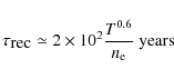
4.5 H I mass function
The H I Mass Function
![]() is
defined as the space density of objects in units of h3Mpc-3. For fitting purposes a Schechter function
(Schechter 1976) can be used of the form:
is
defined as the space density of objects in units of h3Mpc-3. For fitting purposes a Schechter function
(Schechter 1976) can be used of the form:
 |
(15) |
characterised by the parameters
 |
(16) |
![\begin{figure}
\par\includegraphics[width=8.4cm,clip]{11811f26.eps}
\end{figure}](/articles/aa/full_html/2009/34/aa11811-09/img134.png) |
Figure 11: Two-point correlation function of H I-rich objects in our simulation, contrasted with a power-law fit to the observed relation of Meyer et al. (2007). |
| Open with DEXTER | |
The reconstructed structures in our high resolution grids can be used
to determine a simulated H I Mass Function for
structures above ![]()
![]()
![]() .
The result is plotted
in the left panel of Fig. 12, where the H I
Mass Function is shown with a bin size of 0.1 dex. Overlaid is the
best fit to the data, the fitting parameters that have been used are
.
The result is plotted
in the left panel of Fig. 12, where the H I
Mass Function is shown with a bin size of 0.1 dex. Overlaid is the
best fit to the data, the fitting parameters that have been used are
![]() ,
,
![]() and
and
![]() .
Note that in this case the value of
.
Note that in this case the value of
![]() is not very well-constrained, as this parameter defines the
slope of the lower end of the H I Mass Function, but
our simulation is unable to sample the mass function below a mass of
is not very well-constrained, as this parameter defines the
slope of the lower end of the H I Mass Function, but
our simulation is unable to sample the mass function below a mass of
![]() .
The result is compared with
the H I mass function from
Zwaan et al. (2003) (dash-dotted line). The reconstructed mass
function corresponds reasonably well with the mass functions obtained
from galaxies in HIPASS around M*. At masses around 1010
.
The result is compared with
the H I mass function from
Zwaan et al. (2003) (dash-dotted line). The reconstructed mass
function corresponds reasonably well with the mass functions obtained
from galaxies in HIPASS around M*. At masses around 1010![]() ,
the error bars are very large due to small number
statistics. A much larger simulation volume is required to sample this
regime properly. There is a hint of an excess in the simulation near
our resolution limit, this may simply reflect cosmic variance and will
be addressed in future studies. Zwaan et al. (2003) compared
four different quadrants of the southern sky and found that at
,
the error bars are very large due to small number
statistics. A much larger simulation volume is required to sample this
regime properly. There is a hint of an excess in the simulation near
our resolution limit, this may simply reflect cosmic variance and will
be addressed in future studies. Zwaan et al. (2003) compared
four different quadrants of the southern sky and found that at
![]() the estimated space density varies by a factor of
about three, which is comparable to the factor
the estimated space density varies by a factor of
about three, which is comparable to the factor ![]() 2 difference we
see between the simulation and observations.
2 difference we
see between the simulation and observations.
4.5.1 H2 mass function
The H2 Mass Function can be determined in a similar way as the
H I Mass Function. The result is shown in the right
panel of Fig. 12 where the simulated data points are fitted
with a Schechter function. Our best fit parameters are ![]() =
=
![]() ,
,
![]() and
and
![]() .
At the high end of the mass function the results are
affected by low number statistics. The simulated fit is compared with
the fits as determined by Obreschkow & Rawlings (2009) (dashed line)
and Keres et al. (2003) (dash-dotted line). There is very
good agreement over the full mass range.
.
At the high end of the mass function the results are
affected by low number statistics. The simulated fit is compared with
the fits as determined by Obreschkow & Rawlings (2009) (dashed line)
and Keres et al. (2003) (dash-dotted line). There is very
good agreement over the full mass range.
In Fig. 13 the derived H2 masses are plotted as function of
H I mass. The dashed vertical line represents the
completeness limit of H I masses. The data can be
fitted using a power law (solid line) which looks like
![]() with a scaling parameter of
with a scaling parameter of
![]() and a
slope of
and a
slope of
![]() .
.
![\begin{figure}
\par\mbox{\includegraphics[width=8.2cm,clip]{11811f27.eps} \includegraphics[width=8.2cm,clip]{11811f28.eps} }
\end{figure}](/articles/aa/full_html/2009/34/aa11811-09/img147.png) |
Figure 12:
Left panel: H I Mass Function of the
simulated data (black dots) with the best-fit Schechter function
(solid black line), compared with the HIMF from
Zwaan et al. (2003) (dash-dotted red line). Our best fit
line is dashed below
|
| Open with DEXTER | |
4.6 Stars, dark matter and molecular hydrogen
In addition to the SPH-particles, the simulations also contain dark matter and stars. The distribution of these components can be reconstructed and compared with the distribution of neutral hydrogen. For reconstructing the dark matter and stars a very simple adaptive gridding scheme has been used. This gridding scheme was adopted, because the dark matter and star particles do not have a variable smoothing kernel like the gas particles. They do have a smoothing kernel defined by the softening length of 2.5 kpc h-1, however this is a fixed value. The gridding method as described in Sect. 3.3 using a spline kernel can not be used for this reason. Exactly the same regions have been gridded as those previously determined H I objects. First the objects have been gridded with a cell size of 10 kpc using a nearest grid-point algorithm. The resulting moment maps have been used to determine which high density regions contain many particles. In a second step the particles have been gridded to five independent cubes using a 2 kpc cell size. Based on the density of simulation particles in the 10 kpc resolution cube, an individual particle is assigned to one of five different cubes for gridding. The density threshold is determined by the number of particles in the 10 kpc resolution cube integrated along the line of sight. The threshold numbers are 2, 6, 18, 54 and everything above 54 particles respectively. The five cubes are integrated along the line of sight and smoothed using a Gaussian kernel with a standard deviation of 7, 5, 3.5, 2.5 and 1.5 pixels of 2 kpc respectively. Finally the five smoothed maps are added together. These smoothing kernels where chosen to insure that each individual cube covering a different density regime has a smooth density distribution, but preserves as much resolution as practical.
![\begin{figure}
\par\includegraphics[width=8.4cm,clip]{11811f29.eps}
\end{figure}](/articles/aa/full_html/2009/34/aa11811-09/img148.png) |
Figure 13: Derived H2 masses are plotted against H I masses for individual simulated objects. The distribution can be fit using a simple power law (solid (red) line), although the scatter is very large. The dashed vertical line represents the sample cut-off for H I masses in the simulated data. |
| Open with DEXTER | |
In Fig. 14 four examples are shown of the dark matter
and stellar distributions overlaid on the of H I
column density maps. The right panels in this image show the
contours of molecular hydrogen. The stars are concentrated in the
bright and dense parts of the H I objects
corresponding to the bulges and disks of galaxies. The third example
shows an edge-on extended gas disk (its thickness is likely an
artefact of our numerical resolution). The neutral hydrogen is much
more extended than the stars, and the smaller, more diffuse
H I clouds do not have a stellar counterpart in
general. Many objects have H I satellites or
companions, as in the first two examples. These companions or
smaller components do not always have a stellar or molecular
counterpart, although the H I column densities can
reach high values up to
![]() cm-2 as
seen in Galactic high velocity clouds.
cm-2 as
seen in Galactic high velocity clouds.
Interestingly, these H I clouds only occasionally trace dark matter substructures, hence in many cases they are not obvious large-scale accretion events (since the most massive accreting clumps should be accompanied by dark matter). The origin of these diffuse clouds, perhaps analogous to high velocity clouds, may be from a ``halo fountain" of gas cycling in and out of galaxies owing to galactic outflows, as speculated in Oppenheimer & Davé (2008), or represent more diffuse accretion from the extended environment. Studying the kinematics and metallicities of these clouds may reveal signatures of their origin. In the future we plan to investigate such signatures in the simulations to assess how observations of diffuse H I clouds around galaxies can inform our understanding of the processes of galaxy assembly.
![\begin{figure}
\par\mbox{\includegraphics[width=6cm]{figures/11811f30.eps} \incl...
...11f40.eps} \includegraphics[width=6cm]{figures/11811f41.eps} }
\par
\end{figure}](/articles/aa/full_html/2009/34/aa11811-09/img151.png) |
Figure 14:
Column density maps of four reconstructed objects as seen
in neutral hydrogen with contours of Dark Matter ( left panels),
Stars ( middle panels) and molecular hydrogen ( right
panels). For both the Dark Matter and the stars contour levels
are at N = 3, 5, 10, 20, 30, 50 and
|
| Open with DEXTER | |
5 Discussion
To make observational predictions based on numerical simulations, the
first essential step is to establish that the simulation can
adequately reproduce all observational constraints. We have carried
out a critical comparison of our simulated H I data
with observations using a wide range of statistical
measures. Essential in creating simulated data is the minimisation of
the number of free parameters over and above the many that are
already inherent in the simulation;
(Oppenheimer & Davé 2008,2006). In our analysis, the
only additional assumptions we make are that the transitions from
ionised to atomic and from atomic to molecular hydrogen can be
described by a simple threshold effect at two different values of
the thermal pressure, while demanding that the recombination
time be less than the sound-crossing time. The threshold
values are determined by fixing the average H I
density and the density ratio
![]() at
z = 0 to those determined observationally. In choosing this simple
prescription we are strongly limited by current numerical
capabilities. Although we did not solve the complete radiative
transfer problem, we do get quite complex behaviour emerging. The
range of threshold values we explored are consistent with
expected values in literature.
at
z = 0 to those determined observationally. In choosing this simple
prescription we are strongly limited by current numerical
capabilities. Although we did not solve the complete radiative
transfer problem, we do get quite complex behaviour emerging. The
range of threshold values we explored are consistent with
expected values in literature.
The statistics of the reconstructed and observed H
I distributions agree quite well, making it plausible that the
associated H I structures in the simulation may be
similar to those occurring in nature. The simulation cannot reproduce
structures that resemble actual galaxies in detail. Besides the finite
mass resolution of the SPH-particles of ![]()
![]() ,
there are
the inevitable limitations on the included physical processes and their
practical implementation. Nonetheless, we may begin to explore the fate of
partially neutral gas in at least the diffuse outskirts of major galaxies.
,
there are
the inevitable limitations on the included physical processes and their
practical implementation. Nonetheless, we may begin to explore the fate of
partially neutral gas in at least the diffuse outskirts of major galaxies.
Despite the limitations, the simulations can reproduce many observed statistical aspects of H I in galaxies, which is very encouraging for further exploration of this approach. The adopted self-shielding threshold provides good results for this one simulation. Future work will test the variations that are encountered with different feedback mechanisms. The method can also be applied to look at the evolution of neutral hydrogen with redshift. Furthermore, mock observations can be created to make predictions for what future telescopes should detect. This is particularly relevant for assessing performance requirements for the various facilities now under development with a strong H I focus, such as the Square Kilometre Array (SKA) and many of the SKA pathfinders.
5.1 Resolution effects
Table 1: Sensitivity limits for four different telescopes for an assumed line-width of 25 km s-1 after a total integration time of 500 h to image an area of 30 square degrees.
![\begin{figure}
\par\mbox{\includegraphics[angle=270,width=6cm]{figures/11811f42....
...} \includegraphics[angle=270,width=6cm]{figures/11811f44.eps} }
\par\end{figure}](/articles/aa/full_html/2009/34/aa11811-09/img158.png) |
Figure 15: Left panel: simulated object at a distance of 6 Mpc, with a 6 kpc intrinsic beam size. Middle panel: simulated object smoothed to a 8.7 kpc beam size, corresponding to the ASKAP beam at 6 Mpc. Right panel: noise is added corresponding to the ASKAP sensitivity limit after a 500 h observation of 30 square degrees. |
| Open with DEXTER | |
Simulations are limited by their volume and the mass resolution of the particles (over and above the limitations that result from incomplete physics). Although we are able to reconstruct structures of several Mpc in scale, the simulated volume is relatively small. To be able to reconstruct the largest structures encountered in the universe, and effectively overcome cosmic variance, a simulated volume is needed that is about about 300 (rather than 32) Mpc on a side. In the current volume, the most massive structures are suffering from low number statistics. A drawback of using a larger volume is that the mass resolution of individual particles decreases rapidly, making it impossible to resolve structures on even multi-kilo-parsec scales. The approach we have employed to approximate the effects of self-shielding is extremely simple. The actual processes acting on sub-kilo-parsec scales are undoubtedly much more complex. Clumping will occur on the scales of molecular clouds, which will dramatically increase the local densities. The threshold thermal-pressure we determine to approximate the atomic to molecular hydrogen transition only has possible relevance on the kilo-parsec scales of our modelled gas particles. At the smaller physical scales where the transition actually occurs, the physical pressures will likely be substantially different.
We note that realistic simulations of cosmological volumes are extremely challenging, and that even the current state-of-the-art is not particularly successful at reproducing objects that resemble observed galaxies in great detail. The simulation we employ represents a very good compromise between simulations focused on larger and smaller scales. We are mainly interested in the diffuse intergalactic structures on multi-kilo-parsec scales, that would be observable when doing 21-cm H I observations with sufficient sensitivity. We have enough resolution to map and resolve these structures and to reconstruct the extended environments of galaxies and galaxy groups. Our simulation is not suitable for making predictions about the inner cores of galaxies or resolving the star formation process in molecular clouds.
Future work will test our analysis method on both larger and smaller scales. Simulations in a larger volume can provide a more sensitive test of the reconstructed H I Mass function and the two-point correlation function. Simulations in a smaller volume will probably require a more advanced method of modelling the atomic to molecular hydrogen transition. However, substantial insights into the more diffuse phenomena, such as accretion and feedback processes around individual galaxies, are very likely within reach.
5.2 Future observations
This simulation can not only be used for getting a better understanding of the H I distribution, especially at low column densities, but is also very suitable for making predictions for future observations. Currently many radio telescopes are being built as pathfinders toward the SKA. A few examples are the Australia SKA Pathfinder (ASKAP), the Allen Telescope Array (ATA), Karoo Array Telescope (MeerKAT) and the Low frequency array (LOFAR), and many more. Although the SKA will be the final goal, each of these telescopes is a good detector on its own and is planned to be operational in the relatively near future. Of course each telescope will have different characteristics, but in general it will be possible to do surveys deeper, faster and over a broader bandwidth.
We will discuss the simulated maps of two current single dish telescopes, Parkes and Arecibo, and compare these with the capabilities of two future telescopes, the ASKAP and the SKA. Parkes and Arecibo are both single dish telescopes with a multi-beam receiver that have recently been used to do large area surveys, the H I Parkes All Sky Survey (HIPASS, Barnes et al. 2001) and the Arecibo Legacy Fast ALFA Survey (ALFALFA Giovanelli et al. 2005).
To make a fair comparison, all four telescope will get 500 h of observing time to map 30 square degrees of the sky. These numbers are chosen as 500 h is a reasonable time scale to make a deep image and a 30 square degree field is needed to map the extended environment of a galaxy. Furthermore, 30 square degrees is the planned instantaneous field-of-view of ASKAP.
We focus on two cases that illustrate the capabilities of present and upcoming telescopes. In the first example, observations will be simulated at a distance where the beam of the telescopes has a physical size of 25 kpc. This approximate beam size is needed to resolve diffuse filaments and extended companions from the simulation. In the second example observations will be simulated at a fixed distance of 6 Mpc, which is the limiting distance for the Parkes telescope according to the above argument.
Right ascension and declination coordinates are added according to the
distance, centred on an RA of 12 h and a Dec of 0 degrees. For
each telescope the sensitivity is determined that can be achieved
using the given conditions. The technical properties are listed in
Table 1. For the Parkes telescope we use the sensitivity
that is achieved when re-reducing HIPASS data (Popping 2009, in prep.),
which corresponds to ![]() 10 mJy/Beam over 26 km s-1 for a
typical HIPASS field after integrating over
10 mJy/Beam over 26 km s-1 for a
typical HIPASS field after integrating over ![]() 560 s per square
degree. For the Arecibo telescope we used the sensitivity of the
Arecibo Galaxy Environment Survey (AGES) (Auld et al. 2006)
assuming 0.95 mJy/beam over 10 km s-1 after integrating for 10 h per square degree. The expected sensitivities for ASKAP are
described in the initial Array Configuration paper which can be found
on
http://www.atnf.csiro.au/projects/askap/newdocs/configs-3.pdf. ASKAP
is expected to achieve a sensitivity of 7.3 mJy/beam over 21 km s-1 after one hour of integration time. For the SKA we assume a
560 s per square
degree. For the Arecibo telescope we used the sensitivity of the
Arecibo Galaxy Environment Survey (AGES) (Auld et al. 2006)
assuming 0.95 mJy/beam over 10 km s-1 after integrating for 10 h per square degree. The expected sensitivities for ASKAP are
described in the initial Array Configuration paper which can be found
on
http://www.atnf.csiro.au/projects/askap/newdocs/configs-3.pdf. ASKAP
is expected to achieve a sensitivity of 7.3 mJy/beam over 21 km s-1 after one hour of integration time. For the SKA we assume a
![]() m2 K-1 at 2.5 arcmin resolution,
which is 20 times higher than ASKAP. Furthermore we assume a field of
view similar to ASKAP, 30 square degrees instantaneous.
m2 K-1 at 2.5 arcmin resolution,
which is 20 times higher than ASKAP. Furthermore we assume a field of
view similar to ASKAP, 30 square degrees instantaneous.
All the flux densities can be converted into brightness temperature using the equation:
 |
(17) |
where
 |
(18) |
where
 |
(19) |
with
The second column in Table 1 gives the beam size of each telescope, the third column gives the distance at which the beam has a physical size of 25 kpc, and the fourth column gives the physical beam size at a distance of 6 Mpc. The sensitivities in column five are converted to a column density limit when sampling a line of approximately 25 km s-1 width in the last column. We assume that in any analysis only the channels will be selected containing diffuse emission and that the line width of diffuse regions will be of the order of 25 km s-1. Galaxies can have a much larger line-width, however detecting these is not an observational challenge. The reconstructed maps have an intrinsic resolution of 2 kpc with a minimum smoothing kernel size of three pixels. This yields an initial beam size of 6 kpc, which will be smoothed to the appropriate beam size of each telescope, corresponding to the simulated distance. Using the calculated sensitivity limits random Gaussian noise is generated and added to the maps. The steps are shown in Fig. 15, the left panel shows the original reconstructed column density map that is smoothed to the beam of ASKAP in the middle panel. At this stage most of the diffuse and extended emission can still be recognised. Noise is added in the right panel, most of the diffuse emission disappears in the noise.
![\begin{figure}
\par\mbox{\includegraphics[angle=270,width=7.4cm,clip]{11811f45.e...
...4mm}
\includegraphics[angle=270,width=7.4cm,clip]{11811f48.eps} }\end{figure}](/articles/aa/full_html/2009/34/aa11811-09/img170.png) |
Figure 16:
Simulated observations of the same object at a distance at
which the beam size corresponds to 25 kpc for Parkes ( top left),
Arecibo ( top right), ASKAP ( bottom left) and the SKA ( bottom
right). All contours begin at a 3 |
| Open with DEXTER | |
![\begin{figure}
\par\mbox{\includegraphics[angle=270,width=7.4cm,clip]{11811f45.e...
...{4mm}
\includegraphics[angle=270,width=7.4cm,clip]{11811f51.eps} }\end{figure}](/articles/aa/full_html/2009/34/aa11811-09/img171.png) |
Figure 17:
Simulated observations of the same object at a fixed
distance of 6 Mpc for Parkes ( top left), Arecibo ( top right),
ASKAP ( bottom left) and the SKA ( bottom right). Contour
levels start at a 3 |
| Open with DEXTER | |
In Fig. 16 the same field is shown as in Fig. 15, placed at a distance where the beam has a size of 25 kpc. This means that the object looks similar for all four telescopes as it fills the same number of beams, although there is a big difference in angular scale.
For each panel contour levels are drawn starting at 3![]() and increasing as noted in the figure caption, so the actual
values are different in each panel, but can be determined using the
sensitivity limits given in Table 1. All panels look
very similar, as most of the structure and substructure of the
original map is smoothed into two large blobs and essentially all the
diffuse structures are lost in the noise. Only with the SKA can some
extended contours still be recognised at the top of the left
object. However, it is very difficult to distinguish extended emission
from companions, unless the companions are clearly separated by at
least a beam width from the primary object.
and increasing as noted in the figure caption, so the actual
values are different in each panel, but can be determined using the
sensitivity limits given in Table 1. All panels look
very similar, as most of the structure and substructure of the
original map is smoothed into two large blobs and essentially all the
diffuse structures are lost in the noise. Only with the SKA can some
extended contours still be recognised at the top of the left
object. However, it is very difficult to distinguish extended emission
from companions, unless the companions are clearly separated by at
least a beam width from the primary object.
An example of this can be seen in Fig. 17 where the same
object is shown simulated with four telescopes but now at a similar
distance of 6 Mpc. A smaller beam size now yields higher resolution
and more detected structure. The differences between the four panels
are now obvious. Observed with Parkes in the top left panel the object
has essentially no resolved structure. Clearly the beam size is too
large and only suitable for very nearby galaxies, closer than 6
Mpc. Arecibo, with a much smaller beam, can resolve the inner core of
the object and can just detect the brightest companion. Again the
contour levels have values starting at 3![]() ,
so
the outer contour in the top right panel corresponds to
,
so
the outer contour in the top right panel corresponds to
![]() cm-2. ASKAP has a very similar sensitivity
limit as Arecibo with a comparable beam size. However it is notable
that it reaches Arecibo sensitivities with a much smaller collecting
area. Furthermore, these deep integrations have not really been
explored, so the given sensitivities are theoretical limits. It is
very likely that correcting for systematic effects, like the shape of
the spectral bandpass, will be more achievable with an interferometer
like ASKAP rather than a large single dish telescope. In the SKA image
essentially all companions can be clearly distinguished down to a
contour level of
cm-2. ASKAP has a very similar sensitivity
limit as Arecibo with a comparable beam size. However it is notable
that it reaches Arecibo sensitivities with a much smaller collecting
area. Furthermore, these deep integrations have not really been
explored, so the given sensitivities are theoretical limits. It is
very likely that correcting for systematic effects, like the shape of
the spectral bandpass, will be more achievable with an interferometer
like ASKAP rather than a large single dish telescope. In the SKA image
essentially all companions can be clearly distinguished down to a
contour level of ![]()
![]() cm-2. Note that this value
is lower than the 3
cm-2. Note that this value
is lower than the 3![]() value in Table 1, this is
because the beam size of the SKA is smaller than the beam size of the
simulation at a distance of 6 Mpc. To adjust for this we adopt the
beam size of the reconstructed data and smooth the noise to this
larger beam size. In this case the noise value will decrease,
resulting in a higher sensitivity of
value in Table 1, this is
because the beam size of the SKA is smaller than the beam size of the
simulation at a distance of 6 Mpc. To adjust for this we adopt the
beam size of the reconstructed data and smooth the noise to this
larger beam size. In this case the noise value will decrease,
resulting in a higher sensitivity of
![]() cm-2.
cm-2.
6 Conclusion
We have used a hydrodynamic simulation to predict the neutral
hydrogen distribution in the universe. The simulation employs a random
cube of 32 h-1 Mpc on a side at redshift zero, with an SPH mass
resolution of ![]()
![]() .
The physics in the simulation
includes sub-grid treatments of star formation and feedback
mechanisms.
.
The physics in the simulation
includes sub-grid treatments of star formation and feedback
mechanisms.
We have developed a method to extract the neutral hydrogen component
from the total gas budget. At low volume densities the balance is
calculated between photo-ionisation and radiative recombination. For
high densities a correction has to be applied for self-shielding, as
the gas becomes optically thick for ionising photons. In the densest
regions, the atomic hydrogen is turned into molecular hydrogen that
will subsequently form stars. The molecular hydrogen and the
self-shielding transition are both modelled by a critical thermal
pressure. Above the first threshold limit (P/k = 155 cm-3 K),
the gas is assumed to recombine and the neutral fraction is set to
unity. At even higher pressures (P/k = 810 cm-3 K), the atomic
hydrogen is assumed to become molecular hydrogen, so the atomic
fraction becomes zero. These processes only apply to simulated
particles for which the recombination time is shorter than the
sound-crossing time on kpc scales. The two threshold pressures are
tuned to reproduce the observed average H I density
of
![]() Mpc-3 and an
assumed molecular density of
Mpc-3 and an
assumed molecular density of
![]()
![]() Mpc-3, corresponding to a molecular to atomic density
ratio of
Mpc-3, corresponding to a molecular to atomic density
ratio of
![]() .
.
A wide range of statistical comparisons have been made between the reconstructed H I distribution and existing observational constraints including: the two-point correlation function, the H I mass function and the H I column density distribution. There is agreement between all these statistical measures of the observations and the simulations, which is a very encouraging result. Based on this agreement, the simulated H I distribution may be a plausible description of the H I universe, at least on the intermediate spatial scales that are both well-resolved and well-sampled.
We also compare the distribution of neutral and molecular hydrogen with the distribution of dark matter and stars in the simulation. Massive H I structures generally have associated stars, but the more diffuse clouds do not contain large stellar components or in many cases even concentrations of dark matter. The method to extract neutral hydrogen from an SPH output cube can be applied to other simulations, to allow comparison of different models of galaxy formation. Furthermore, the results can be used to create mock observations and make predictions for future observations. This preliminary study shows that as H I observations of diffuse gas outside of galactic disks continue to improve, simulations will play a vital role in guiding and interpreting such data to help us better understand the role that H I plays in galaxy formation.
Acknowledgements
We would like to thank Thijs van der Hulst for useful discussions and comments on the original manuscript. We appreciate the constructive comments of the anonymous referee.
References
- Auld, R., Minchin, R. F., Davies, J. I., et al. 2006, MNRAS, 371, 1617 [NASA ADS] [CrossRef] (In the text)
- Barnes, D. G., Staveley-Smith, L., de Blok, W. J. G., et al. 2001, MNRAS, 322, 486 [NASA ADS] [CrossRef] (In the text)
- Blitz, L., & Rosolowsky, E. 2004, ApJ, 612, L29 [NASA ADS] [CrossRef] (In the text)
- Blitz, L., & Rosolowsky, E. 2006, ApJ, 650, 933 [NASA ADS] [CrossRef] (In the text)
- Boulares, A., & Cox, D. P. 1990, ApJ, 365, 544 [NASA ADS] [CrossRef] (In the text)
- Braun, R., & Thilker, D. A. 2004, A&A, 417, 421 [NASA ADS] [CrossRef] [EDP Sciences] (In the text)
- Cen, R., & Ostriker, J. P. 1999, ApJ, 514, 1 [NASA ADS] [CrossRef]
- Corbelli, E., & Bandiera, R. 2002, ApJ, 567, 712 [NASA ADS] [CrossRef] (In the text)
- Davé, R., & Tripp, T. M. 2001, ApJ, 553, 528 [NASA ADS] [CrossRef] (In the text)
- Davé, R., Hernquist, L., Katz, N., & Weinberg, D. H. 1999, ApJ, 511, 521 [NASA ADS] [CrossRef]
- Davé, R., Cen, R., Ostriker, J. P., et al. 2001, ApJ, 552, 473 [NASA ADS] [CrossRef]
- Davé, R., Finlator, K., & Oppenheimer, B. D. 2006, MNRAS, 370, 273 [NASA ADS] (In the text)
- Davé, R., Oppenheimer, B. D., & Sivanandam, S. 2008, MNRAS, 391, 110 [NASA ADS] [CrossRef] (In the text)
- Davis, M., & Huchra, J. 1982, ApJ, 254, 437 [NASA ADS] [CrossRef]
- Dekel, A., Birnboim, Y., Engel, G., et al. 2009, Nature, 457, 451 [NASA ADS] [CrossRef]
- Dove, J. B., & Shull, J. M. 1994, ApJ, 423, 196 [NASA ADS] [CrossRef] (In the text)
- Eisenstein, D. J., & Hu, W. 1999, ApJ, 511, 5 [NASA ADS] [CrossRef] (In the text)
- Finlator, K., & Davé, R. 2008, MNRAS, 385, 2181 [NASA ADS] [CrossRef] (In the text)
- Fukugita, M., Hogan, C. J., & Peebles, P. J. E. 1998, ApJ, 503, 518 [NASA ADS] [CrossRef] (In the text)
- Giovanelli, R., Haynes, M. P., Kent, B. R., et al. 2005, AJ, 130, 2598 [NASA ADS] [CrossRef] (In the text)
- Groth, E. J., & Peebles, P. J. E. 1977, ApJ, 217, 385 [NASA ADS] [CrossRef]
- Haardt, F., & Madau, P. 2001, in Clusters of Galaxies and the High Redshift Universe Observed in X-rays (In the text)
- Keres, D., Yun, M. S., & Young, J. S. 2003, ApJ, 582, 659 [NASA ADS] [CrossRef] (In the text)
- Keres, D., Katz, N., Weinberg, D. H., & Davé, R. 2005, MNRAS, 363, 2 [NASA ADS] [CrossRef]
- Keres, D., Katz, N., Fardal, M., Dave, R., & Weinberg, D. H. 2009, MNRAS, 395, 160 [NASA ADS] [CrossRef]
- Landy, S. D., & Szalay, A. S. 1993, ApJ, 412, 64 [NASA ADS] [CrossRef] (In the text)
- Mellema, G., Iliev, I. T., Pen, U.-L., & Shapiro, P. R. 2006, MNRAS, 372, 679 [NASA ADS] [CrossRef] (In the text)
- Meyer, M. J., Zwaan, M. A., Webster, R. L., Brown, M. J. I., & Staveley-Smith, L. 2007, ApJ, 654, 702 [NASA ADS] [CrossRef] (In the text)
- Monaghan, J. J., & Lattanzio, J. C. 1985, A&A, 149, 135 [NASA ADS] (In the text)
- Murray, N., Quataert, E., & Thompson, T. A. 2005, ApJ, 618, 569 [NASA ADS] [CrossRef] (In the text)
- Noordermeer, E., van der Hulst, J. M., Sancisi, R., Swaters, R. A., & van Albada, T. S. 2005, A&A, 442, 137 [NASA ADS] [CrossRef] [EDP Sciences]
- Norberg, P., Baugh, C. M., Hawkins, E., et al. 2002, MNRAS, 332, 827 [NASA ADS] [CrossRef] (In the text)
- Obreschkow, D., & Rawlings, S. 2009, MNRAS, 394, 1857 [NASA ADS] [CrossRef] (In the text)
- Oppenheimer, B. D., & Davé, R. 2006, MNRAS, 373, 1265 [NASA ADS] [CrossRef]
- Oppenheimer, B. D., & Davé, R. 2008, MNRAS, 387, 577 [NASA ADS] [CrossRef]
- Oppenheimer, B. D., & Davé, R. 2009, MNRAS, 395, 1875 [NASA ADS] [CrossRef]
- Osterbrock, D. E. 1989, Astrophysics of gaseous nebulae and active galactic nuclei, Research supported by the University of California, John Simon Guggenheim Memorial Foundation, University of Minnesota, et al. (Mill Valley, CA: University Science Books), 422 (In the text)
- Pelupessy, F. I. 2005, Ph.D. thesis, Leiden University (In the text)
- Pontzen, A., Governato, F., Pettini, M., et al. 2008, MNRAS, 390, 1349 [NASA ADS] (In the text)
- Rosenberg, J. L., & Schneider, S. E. 2002, ApJ, 567, 247 [NASA ADS] [CrossRef] (In the text)
- Schechter, P. 1976, ApJ, 203, 297 [NASA ADS] [CrossRef] (In the text)
- Spergel, D. N., Bean, R., Doré, O., et al. 2007, ApJS, 170, 377 [NASA ADS] [CrossRef] (In the text)
- Springel, V., & Hernquist, L. 2002, MNRAS, 333, 649 [NASA ADS] [CrossRef] (In the text)
- Springel, V., & Hernquist, L. 2003a, MNRAS, 339, 289 [NASA ADS] [CrossRef] (In the text)
- Springel, V., & Hernquist, L. 2003b, MNRAS, 339, 312 [NASA ADS] [CrossRef] (In the text)
- Swaters, R. A., van Albada, T. S., van der Hulst, J. M., & Sancisi, R. 2002, A&A, 390, 829 [NASA ADS] [CrossRef] [EDP Sciences] (In the text)
- Tielens, A. G. G. M. 2005, The Physics and Chemistry of the Interstellar Medium (In the text)
- Verner, D. A., & Ferland, G. J. 1996, ApJS, 103, 467 [NASA ADS] [CrossRef] (In the text)
- Walterbos, R. A. M., & Braun, R. 1996, in The Minnesota Lectures on Extragalactic Neutral Hydrogen, 106, 1 (In the text)
- Weinberg, D. H., Miralda-Escude, J., Hernquist, L., & Katz, N. 1997, ApJ, 490, 564 [NASA ADS] [CrossRef] (In the text)
- Wolfire, M. G., McKee, C. F., Hollenbach, D., & Tielens, A. G. G. M. 2003, ApJ, 587, 278 [NASA ADS] [CrossRef] (In the text)
- Wong, T., & Blitz, L. 2002, ApJ, 569, 157 [NASA ADS] [CrossRef] (In the text)
- Zehavi, I., Eisenstein, D. J., Nichol, R. C., et al. 2005, ApJ, 621, 22 [NASA ADS] [CrossRef] (In the text)
- Zheng, Z., & Miralda-Escudé, J. 2002, ApJ, 568, L71 [NASA ADS] [CrossRef] (In the text)
- Zwaan, M. A., Staveley-Smith, L., Koribalski, B. S., et al. 2003, AJ, 125, 2842 [NASA ADS] [CrossRef] (In the text)
- Zwaan, M. A., van der Hulst, J. M., Briggs, F. H., Verheijen, M. A. W., & Ryan-Weber, E. V. 2005, MNRAS, 364, 1467 [NASA ADS] [CrossRef] (In the text)
All Tables
Table 1: Sensitivity limits for four different telescopes for an assumed line-width of 25 km s-1 after a total integration time of 500 h to image an area of 30 square degrees.
All Figures
| |
Figure 1: Neutral fraction as a function of density for different temperatures between 104 and 109 K. |
| Open with DEXTER | |
| In the text | |
| |
Figure 2: Temperatures are plotted against densities for every 200 th. particle in the simulation. The dashed (blue) and dash-dotted (red) lines correspond to constant thermal pressures of P/k = 155 and 810 cm-3 K, that were found empirically to reproduce the observed mass densities of atomic and molecular gas at z = 0. The solid (green) line shows where the recombination time is equal to the sound-crossing time at a physical scale of one kpc. Particles above/left of the green line are unlikely to be neutral or molecular. |
| Open with DEXTER | |
| In the text | |
| |
Figure 3:
The average molecular density at z = 0 is plotted
against the threshold thermal pressure, where molecular hydrogen
is assumed to form from atomic, while also satisfying the
condition that
|
| Open with DEXTER | |
| In the text | |
| |
Figure 4:
The average H I mass density at
z = 0 is plotted against the threshold thermal pressure, where
atomic hydrogen is assumed to recombine from ionised, while also
satisfying the condition that
|
| Open with DEXTER | |
| In the text | |
| |
Figure 5: Left panel: H I distribution function after gridding to 80 kpc (dashed (red) line). The solid (blue) line corresponds to data gridded to a 2 kpc cell size. Filled dots correspond to the QSO absorption line data (Corbelli & Bandiera 2002). Right panel: combined H I distribution functions of the simulation, gridded to a resolution of 2 kpc (solid (blue) line) and 80 kpc (dashed (purple) line). Overlaid are distribution function from observational data of M 31 (Braun & Thilker 2004), WHISP (Swaters et al. 2002; Zwaan et al. 2005) and QSO absorption lines (Corbelli & Bandiera 2002) respectively. The reconstructed H I distribution function corresponds very well to all observed distribution functions. |
| Open with DEXTER | |
| In the text | |
| |
Figure 6:
Fractional area of reconstructed H I
(dashed line, right-hand axis) and cumulated surface area (solid
line, left-hand axis) plotted against column density on a
logarithmic scale with a bin size of
|
| Open with DEXTER | |
| In the text | |
| |
Figure 7: Top left panel: column density of total H gas integrated over a depth of 32 h-1 Mpc on a logarithmic scale, gridded to a resolution of 80 kpc. Top right panel: molecular hydrogen component. Only very dense regions in the total hydrogen component contain molecular hydrogen. Bottom panel: neutral atomic hydrogen component of the same region. In the neutral hydrogen distribution the highest densities are comparable to the densities in the total hydrogen distribution, but there is a very sharp transition to low neutral column densities as the gas becomes optically thin. Note the very different scales, the total hydrogen spanning only 2 orders of magnitude and the neutral hydrogen, eight. |
| Open with DEXTER | |
| In the text | |
| |
Figure 8:
Four examples of high density regions in the reconstructed
data, gridded to a cell size of 2 kpc. The left panels show the
total hydrogen, while the middle panels show only the neutral
component. Some objects have many satellites, as in the top
panels, while others are much more isolated. All examples have
extended H I at column densities around
|
| Open with DEXTER | |
| In the text | |
| |
Figure 9:
Neutral fraction plotted against H I
column density. The colour-bar represents the probability of detecting a
certain combination of H I column density and
neutral fraction on logarithmic scale. At the highest densities
|
| Open with DEXTER | |
| In the text | |
| |
Figure 10:
Left panel: cumulative mass of total hydrogen as function
of column density, the different phases are shown with different
colours. The Ly |
| Open with DEXTER | |
| In the text | |
| |
Figure 11: Two-point correlation function of H I-rich objects in our simulation, contrasted with a power-law fit to the observed relation of Meyer et al. (2007). |
| Open with DEXTER | |
| In the text | |
| |
Figure 12:
Left panel: H I Mass Function of the
simulated data (black dots) with the best-fit Schechter function
(solid black line), compared with the HIMF from
Zwaan et al. (2003) (dash-dotted red line). Our best fit
line is dashed below
|
| Open with DEXTER | |
| In the text | |
| |
Figure 13: Derived H2 masses are plotted against H I masses for individual simulated objects. The distribution can be fit using a simple power law (solid (red) line), although the scatter is very large. The dashed vertical line represents the sample cut-off for H I masses in the simulated data. |
| Open with DEXTER | |
| In the text | |
| |
Figure 14:
Column density maps of four reconstructed objects as seen
in neutral hydrogen with contours of Dark Matter ( left panels),
Stars ( middle panels) and molecular hydrogen ( right
panels). For both the Dark Matter and the stars contour levels
are at N = 3, 5, 10, 20, 30, 50 and
|
| Open with DEXTER | |
| In the text | |
| |
Figure 15: Left panel: simulated object at a distance of 6 Mpc, with a 6 kpc intrinsic beam size. Middle panel: simulated object smoothed to a 8.7 kpc beam size, corresponding to the ASKAP beam at 6 Mpc. Right panel: noise is added corresponding to the ASKAP sensitivity limit after a 500 h observation of 30 square degrees. |
| Open with DEXTER | |
| In the text | |
| |
Figure 16:
Simulated observations of the same object at a distance at
which the beam size corresponds to 25 kpc for Parkes ( top left),
Arecibo ( top right), ASKAP ( bottom left) and the SKA ( bottom
right). All contours begin at a 3 |
| Open with DEXTER | |
| In the text | |
| |
Figure 17:
Simulated observations of the same object at a fixed
distance of 6 Mpc for Parkes ( top left), Arecibo ( top right),
ASKAP ( bottom left) and the SKA ( bottom right). Contour
levels start at a 3 |
| Open with DEXTER | |
| In the text | |
Copyright ESO 2009
Current usage metrics show cumulative count of Article Views (full-text article views including HTML views, PDF and ePub downloads, according to the available data) and Abstracts Views on Vision4Press platform.
Data correspond to usage on the plateform after 2015. The current usage metrics is available 48-96 hours after online publication and is updated daily on week days.
Initial download of the metrics may take a while.