| Issue |
A&A
Volume 502, Number 2, August I 2009
|
|
|---|---|---|
| Page(s) | L1 - L4 | |
| Section | Letters | |
| DOI | https://doi.org/10.1051/0004-6361/200911997 | |
| Published online | 02 July 2009 | |
LETTER TO THE EDITOR
Impact of granulation effects on the use of Balmer lines as temperature indicators![[*]](/icons/foot_motif.png)
H.-G. Ludwig1,2 - N. T. Behara1,2 - M. Steffen3 - P. Bonifacio1,2,4
1 - CIFIST Marie Curie Excellence Team, France
2 -
GEPI, Observatoire de Paris, CNRS, Université Paris Diderot, 92195 Meudon Cedex, France
3 -
Astrophysikalisches Institut Potsdam, An der Sternwarte 16, 14482 Potsdam, Germany
4 -
Istituto Nazionale di Astrofisica, Osservatorio Astronomico di Trieste, via Tiepolo 11, 34143 Trieste, Italy
Received 6 March 2009 / Accepted 19 May 2009
Abstract
Context. Balmer lines serve as important indicators of stellar effective temperatures in late-type stellar spectra. One of their modelling uncertainties is the influence of convective flows on their shape.
Aims. We aim to characterize the influence of convection on the wings of Balmer lines.
Methods. We perform a differential comparison of synthetic Balmer line profiles obtained from 3D hydrodynamical model atmospheres and 1D hydrostatic standard ones. The model parameters are appropriate for F, G, K dwarf and subgiant stars of metallicity ranging from solar to 10-3 solar.
Results. The shape of the Balmer lines predicted by 3D models can never be exactly reproduced by a 1D model, irrespective of its effective temperature. We introduce the concept of a 3D temperature correction, as the effective temperature difference between a 3D model and a 1D model which provides the closest match to the 3D profile. The temperature correction is different for the different members of the Balmer series and depends on the adopted mixing-length parameter
![]() in the 1D model. Among the investigated models, the 3D correction ranges from -300 K to +300 K. Horizontal temperature fluctuations tend to reduce the 3D correction.
in the 1D model. Among the investigated models, the 3D correction ranges from -300 K to +300 K. Horizontal temperature fluctuations tend to reduce the 3D correction.
Conclusions. Accurate effective temperatures cannot be derived from the wings of Balmer lines, unless the effects of convection are properly accounted for. The 3D models offer a physically well justified way of doing so. The use of 1D models treating convection with the mixing-length theory do not appear to be suitable for this purpose. In particular, there are indications that it is not possible to determine a single value of
![]() which will optimally reproduce the Balmer lines for any choice of atmospheric parameters. The investigation of a more extended grid and direct comparison with observed Balmer profiles will be carried out in the near future.
which will optimally reproduce the Balmer lines for any choice of atmospheric parameters. The investigation of a more extended grid and direct comparison with observed Balmer profiles will be carried out in the near future.
Key words: hydrodynamics - convection - radiative transfer - stars: atmospheres - line: profiles - methods: numerical
1 Introduction
Balmer lines are prominent features in stellar spectra. There has been a long tradition of using the Balmer line wings for the determination of effective temperatures of F-K stars (a non-exhaustive list includes: Soderblom 1986; Cayrel et al. 1985; Gehren 1981; Strohbach 1970; Searle & Oke 1962; Cayrel de Strobel 1960). However, the use of Balmer lines as temperature indicators requires fairly high quality spectra and a sophisticated theoretical framework, both from the point of view of micro-physics and of the model atmospheres employed. It was not until the comprehensive work of Fuhrmann et al. (1993) that the wings of Balmer lines became the temperature indicator of choice in many investigations. One of the advantages of Balmer line temperatures is that, unlike those based on colours or on the infrared flux method, they are reddening independent and may, in principle, provide an accuracy of the order of 50 K.
In the framework of 1D homogeneous model atmospheres, in which convective energy transport is described by the mixing-length approximation (Böhm-Vitense 1958), Fuhrmann et al. (1993) studied in detail the effects of convection on the wings of the Balmer lines. They convincingly demonstrated that, as a consequence of their different depth of formation, the response to a change in the adopted mixing-length parameter
![]() of the various members of the Balmer sequence is different.
The first line of the series, H
of the various members of the Balmer sequence is different.
The first line of the series, H
![]() ,
is fairly insensitive to the choice of
,
is fairly insensitive to the choice of
![]() ,
at least
for solar metallicity models, but the higher members are fairly sensitive. This provides, in principle, a way to select the most appropriate value of
,
at least
for solar metallicity models, but the higher members are fairly sensitive. This provides, in principle, a way to select the most appropriate value of
![]() .
For a star for which the effective temperature is known, like the Sun, one may select the
.
For a star for which the effective temperature is known, like the Sun, one may select the
![]() which best reproduces all members of the Balmer series.
which best reproduces all members of the Balmer series.
At the time Fuhrmann et al. (1993) performed their investigation, hydrodynamical simulations in which convection is treated in a physical and non-parameterized way had just become available (Nordlund & Stein 1991; Steffen 1991). However, there were not enough simulations to cover satisfactorily the range of
![]() and
and
![]() which was pertinent to their investigation; moreover those simulations were not very sophisticated in the treatment of line opacity. After 15 years the situation has greatly improved. Full three dimensional hydrodynamical simulations (hereafter 3D models, for short) and the associated line-formation codes have reached a level of sophistication in radiative
transfer comparable to that of state-of-the art 1D models and line-formation codes. More importantly, for the first time a fairly large grid of 3D models is available to allow
a systematic investigation of convection effects.
which was pertinent to their investigation; moreover those simulations were not very sophisticated in the treatment of line opacity. After 15 years the situation has greatly improved. Full three dimensional hydrodynamical simulations (hereafter 3D models, for short) and the associated line-formation codes have reached a level of sophistication in radiative
transfer comparable to that of state-of-the art 1D models and line-formation codes. More importantly, for the first time a fairly large grid of 3D models is available to allow
a systematic investigation of convection effects.
To clarify how the results of Fuhrmann et al. (1993) may be affected by inhomogeneities, we investigate Balmer line formation in hydrodynamical model atmospheres. Broadening due to convective velocities is only important in the inner line cores of Balmer lines; in this sense, the outer parts of the Balmer lines are particularly well suited sensors of the thermal structure of an atmosphere. We use a sample of 3D model atmospheres covering the range [M/H] = -3.0 to 0.0 in metallicity, 5500-6550 K in
![]() and 3.5-4.5 in
and 3.5-4.5 in
![]() .
Our investigation is purely theoretical, and we express our results in terms of effective temperature differences between 3D and 1D models.
.
Our investigation is purely theoretical, and we express our results in terms of effective temperature differences between 3D and 1D models.
2 Model atmospheres and line formation
The 3D model atmospheres we use have been computed with the CO5BOLD code (Wedemeyer et al. 2004; Freytag et al. 2002,2008). The code solves the time-dependent equations of compressible hydrodynamics coupled to radiative transfer in a constant gravity field in a Cartesian computational domain which is representative of a volume located at the stellar surface. Further details on computational methods and validity tests can be found in Ludwig et al. (2009). In Table 1 we provide some of the basic properties of the 3D models employed in this paper.
Table 1: Parameters of the 3D models.
In order to make our comparison strictly differential we employed as a reference 1D models computed with the LHD code, which employs the same microphysics and numerical scheme for radiative transfer as CO5BOLD. Further details on these models can be found in Caffau & Ludwig (2007).
These models are classical hydrostatic 1D models; no velocity fields are considered,
convection is treated using the Mihalas (1978) formulation of the mixing-length theory,
and one has to assume a microturbulence parameter in associated spectral synthesis calculations.
We refer to these models as
![]() .
.
In addition we employed the 1D structure which is obtained by a temporal and spatial average of the 3D models over surfaces of constant Rosseland optical depth. We refer to these models as
![]() .
The
.
The
![]() model has, by construction, the mean temperature profile of the 3D model, but no horizontal
temperature fluctuations are present. Therefore, a comparison
model has, by construction, the mean temperature profile of the 3D model, but no horizontal
temperature fluctuations are present. Therefore, a comparison
![]() highlights the effects of such fluctuations, a comparison
highlights the effects of such fluctuations, a comparison
![]() highlights the effect of differences in the temperature profiles, and the
highlights the effect of differences in the temperature profiles, and the
![]() comparison provides insight into the combined effects of different temperature profiles and horizontal temperature fluctuations.
comparison provides insight into the combined effects of different temperature profiles and horizontal temperature fluctuations.
The Balmer line profiles have been computed with the Linfor3D code![]() . In the version of the code used here, the Balmer line profiles are computed with the theory of Cayrel & Traving (1960). In the future, more up-dated theories will be implemented in Linfor3D. However, for the purpose of our strictly differential analysis, the theory employed should not be relevant. Linfor3D is capable of
computing line profiles both for 3D and 1D models. The 3D synthesis is very CPU time demanding. For this reason, we computed for each line only a range of 5.5 nm around the line center at a resolution of 1.5
. In the version of the code used here, the Balmer line profiles are computed with the theory of Cayrel & Traving (1960). In the future, more up-dated theories will be implemented in Linfor3D. However, for the purpose of our strictly differential analysis, the theory employed should not be relevant. Linfor3D is capable of
computing line profiles both for 3D and 1D models. The 3D synthesis is very CPU time demanding. For this reason, we computed for each line only a range of 5.5 nm around the line center at a resolution of 1.5 ![]() 10-2 nm. Furthermore, we did not include any blending lines in the wings of the Balmer profiles. While this clearly limits the accuracy with which the higher members of the series can reproduce the observations of more metal-rich stars, it is not relevant for the present differential theoretical comparison.
10-2 nm. Furthermore, we did not include any blending lines in the wings of the Balmer profiles. While this clearly limits the accuracy with which the higher members of the series can reproduce the observations of more metal-rich stars, it is not relevant for the present differential theoretical comparison.
![\begin{figure}
\par\includegraphics[width=8.5cm,clip]{11997fg1.ps}
\end{figure}](/articles/aa/full_html/2009/29/aa11997-09/img29.png) |
Figure 1:
H
|
3 3D temperature correction
To quantify the granulation effects, we use the concept of a 3D temperature correction. This is defined as the difference between the effective temperature of a 3D model and the temperature derived by fitting Balmer line profiles computed from a
![]() sequence of
sequence of
![]() models with the same surface gravity and metallicity to the corresponding 3D profile. The 3D temperature correction is in general different for the different members of the Balmer series (here we investigate only the first three members) and depends on the
models with the same surface gravity and metallicity to the corresponding 3D profile. The 3D temperature correction is in general different for the different members of the Balmer series (here we investigate only the first three members) and depends on the
![]() adopted for the
adopted for the
![]() models. Although we believe that the 3D temperature correction is a useful description, one should bear in mind that it is a
simplification. In general, the whole profile computed from a 3D model has a different shape from that of a 1D model; an example is given in Fig. 1. No profile computed from a 1D model, whatever the temperature, can exactly reproduce the profile computed from the 3D model. The
temperature correction singles out the 1D model that provides the profile nearest to the profile computed from the 3D model. Clearly, the concept of distance (near or far) has to be defined by a suitable metric.
models. Although we believe that the 3D temperature correction is a useful description, one should bear in mind that it is a
simplification. In general, the whole profile computed from a 3D model has a different shape from that of a 1D model; an example is given in Fig. 1. No profile computed from a 1D model, whatever the temperature, can exactly reproduce the profile computed from the 3D model. The
temperature correction singles out the 1D model that provides the profile nearest to the profile computed from the 3D model. Clearly, the concept of distance (near or far) has to be defined by a suitable metric.
As a measure of the similarity, we used the root-mean-square deviation
![]() between the
normalized line profiles above a prescribed residual flux level,
between the
normalized line profiles above a prescribed residual flux level,
![\begin{displaymath}%
\ensuremath{\Delta_{\rm rms}} ^2 \equiv \frac{1}{N} \sum_{i...
...{\rm 3D}_i -
f^{\rm 1D}_i(\ensuremath{T_{\rm eff}} )\right]^2
\end{displaymath}](/articles/aa/full_html/2009/29/aa11997-09/img31.png) |
(1) |
where N is the number data points making up the line profile,
To calculate
![]() one has to define the portion of the profile over which this is computed.
The line core must always be excluded in these comparisons, since in real stars it is affected
by the presence of a chromosphere. When fitting theoretical to observed spectra, the usual
choice is to define a wavelength interval which defines the wings of the line. Typical choices are 0.3 nm and 0.5 nm from line centre (Cayrel et al. 1985). In the comparison of theoretical spectra,
however, we may take advantage of the fact that the continuum is perfectly defined and consider the wings as the portion of the profile that is above a given threshold. In this way a similar fraction of the line wing is considered, irrespective of the temperature of the star. We believe this choice is the most appropriate for the comparison of theoretical spectra, and use a threshold of 0.8 in residual flux.
one has to define the portion of the profile over which this is computed.
The line core must always be excluded in these comparisons, since in real stars it is affected
by the presence of a chromosphere. When fitting theoretical to observed spectra, the usual
choice is to define a wavelength interval which defines the wings of the line. Typical choices are 0.3 nm and 0.5 nm from line centre (Cayrel et al. 1985). In the comparison of theoretical spectra,
however, we may take advantage of the fact that the continuum is perfectly defined and consider the wings as the portion of the profile that is above a given threshold. In this way a similar fraction of the line wing is considered, irrespective of the temperature of the star. We believe this choice is the most appropriate for the comparison of theoretical spectra, and use a threshold of 0.8 in residual flux.
In addition to the best matching
![]() of a 1D model, the fitting provided further information: i) the overall quality of the fit is related to the residual
of a 1D model, the fitting provided further information: i) the overall quality of the fit is related to the residual
![]() at the best matching
at the best matching
![]() ;
ii) the sensitivity to which we can determine
;
ii) the sensitivity to which we can determine
![]() is related to the rate of change of
is related to the rate of change of
![]() (more precisely its curvature) with respect to
(more precisely its curvature) with respect to
![]() at the matching point. Since we are dealing here with theoretical, essentially noise-less data, the sensitivity is not a real issue, and we can fix the best matching
at the matching point. Since we are dealing here with theoretical, essentially noise-less data, the sensitivity is not a real issue, and we can fix the best matching
![]() to arbitrary precision. However, in practice one is usually working with spectra of only finite signal-to-noise ratio (S/N) so that the sensitivity is important for the precision to which
to arbitrary precision. However, in practice one is usually working with spectra of only finite signal-to-noise ratio (S/N) so that the sensitivity is important for the precision to which
![]() can be obtained. To make a connection to the practical limitations, we present sensitivities and qualities of the fits in a form which makes it easy to relate them to the situation one encounters in finite S/N spectra.
can be obtained. To make a connection to the practical limitations, we present sensitivities and qualities of the fits in a form which makes it easy to relate them to the situation one encounters in finite S/N spectra.
We assume a simple noise model where all pixels have the same S/N distributed according to Gaussian statistics. This is well justified since all pixels have a rather similar flux level due to our chosen high flux threshold in the fitting. The standard deviation of the Gaussian distribution of the flux
![]() is given by
is given by
![]() .
Our minimization of
.
Our minimization of
![]() would then transform to a
would then transform to a
![]() -minimization.
-minimization.
![]() is related to
is related to
![]() as
as
![]() where N is the number of points which sample the line profile. The uncertainty of the fitted effective temperature
where N is the number of points which sample the line profile. The uncertainty of the fitted effective temperature
![]() is given by (e.g., Press et al. 1992)
is given by (e.g., Press et al. 1992)
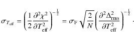
Not surprisingly, the attainable precision scales inversely proportionally to the S/N, and to
In a similar vein, we express the quality of the fit QF related to the residual
![]() at the fitting point in terms of a temperature difference
at the fitting point in terms of a temperature difference
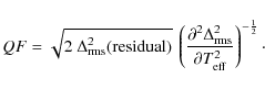
This provides a handy measure of whether the derived 3D
4 Results
For each 3D model, the 3D temperature correction (![]() ), the quality of fit (QF) and the sensitivity (
), the quality of fit (QF) and the sensitivity (
![]() )
for three different grids of LHD models corresponding to three choices of
)
for three different grids of LHD models corresponding to three choices of
![]() are listed in Table 2. The last nine columns of the table provide the same quantities, but for the
are listed in Table 2. The last nine columns of the table provide the same quantities, but for the
![]() model. These allow us to understand what part of the 3D temperature correction can be ascribed to differences in the mean temperature profiles of a 3D model and
model. These allow us to understand what part of the 3D temperature correction can be ascribed to differences in the mean temperature profiles of a 3D model and
![]() model. Graphical representations of the results are provided in the online Appendices.
model. Graphical representations of the results are provided in the online Appendices.
Table 2:
3D corrections, ![]() ,
the quality of fit, QF, and the sensitivity of the fit,
,
the quality of fit, QF, and the sensitivity of the fit,
![]() for the different models in units of K.
for the different models in units of K.
The sample of investigated models is not large, however several patterns in the temperature corrections clearly emerge. At solar metallicity,
![]() = 0.5 provides nearly the same temperature correction for the first three Balmer lines. This result matches what was derived from the comparison of observed spectra to theoretical spectra based on 1D models by Fuhrmann et al. (1993) and van't Veer-Menneret & Megessier (1996). We also find that the wings of H
= 0.5 provides nearly the same temperature correction for the first three Balmer lines. This result matches what was derived from the comparison of observed spectra to theoretical spectra based on 1D models by Fuhrmann et al. (1993) and van't Veer-Menneret & Megessier (1996). We also find that the wings of H![]() are relatively insensitive to
are relatively insensitive to
![]() .
In the past this has motivated the use of only H
.
In the past this has motivated the use of only H![]() ,
but not of higher members of the series, for the determination of
,
but not of higher members of the series, for the determination of
![]() (Asplund et al. 2006; Bonifacio et al. 2007). At low metallicity, however, the insensitivity is lost, and the temperature correction of H
(Asplund et al. 2006; Bonifacio et al. 2007). At low metallicity, however, the insensitivity is lost, and the temperature correction of H![]() is not independent of
is not independent of
![]() .
There are also sizeable differences in the temperature corrections of the various Balmer lines.
.
There are also sizeable differences in the temperature corrections of the various Balmer lines.
In Table 3 we provide the temperature correction spread ![]() ,
defined as
,
defined as
![]() among the first three lines of the Balmer series. For the models at
among the first three lines of the Balmer series. For the models at
![]() = 5500 K and
= 5500 K and
![]() = 5920 K the smallest spread is achieved for
= 5920 K the smallest spread is achieved for
![]() = 2.0. For the
= 2.0. For the
![]() = 5500 K model the spread in the temperature correction is not even a monotonic function of
= 5500 K model the spread in the temperature correction is not even a monotonic function of
![]() .
However, the spread for
.
However, the spread for
![]() = 2.0 is not considerably smaller than that for
= 2.0 is not considerably smaller than that for
![]() = 0.5, especially when compared to the associated errors. This is not surprising; the mixing-length theory is a parametric phenomenological description of convection and it is obvious that it is not possible for a single value of the free parameter to capture all the complexity of this physical phenomenon. It can be seen that the situation is more complicated for the cooler models, while for the three models hotter than 6000 K,
= 0.5, especially when compared to the associated errors. This is not surprising; the mixing-length theory is a parametric phenomenological description of convection and it is obvious that it is not possible for a single value of the free parameter to capture all the complexity of this physical phenomenon. It can be seen that the situation is more complicated for the cooler models, while for the three models hotter than 6000 K, ![]() is a monotonic value of
is a monotonic value of
![]() and achieves the smallest value for
and achieves the smallest value for
![]() = 0.5.
= 0.5.
The
![]() differences appear to be quite regular: the lower the temperature, the higher the temperature correction, reaching the value of 500 K for the model at
differences appear to be quite regular: the lower the temperature, the higher the temperature correction, reaching the value of 500 K for the model at
![]() = 5500 K. This regularity is not immediately obvious when looking at the
= 5500 K. This regularity is not immediately obvious when looking at the
![]() differences, since these depend also on the temperature fluctuation. The importance of temperature fluctuations is different for the different
differences, since these depend also on the temperature fluctuation. The importance of temperature fluctuations is different for the different
![]() ,
but also for different metallicities and gravities. In all cases we see that the role of the temperature fluctuations is to reduce the temperature correction, with respect to what is derived with respect to the
,
but also for different metallicities and gravities. In all cases we see that the role of the temperature fluctuations is to reduce the temperature correction, with respect to what is derived with respect to the
![]() model. But this reduction can be as large as 50% (for the
model. But this reduction can be as large as 50% (for the
![]() = 5500 K model) or as small as 7% (for the
= 5500 K model) or as small as 7% (for the
![]() = 5920 K model).
= 5920 K model).
Table 3:
Spread of ![]() among Balmer series members.
among Balmer series members.
5 Conclusions
The main conclusion that can be drawn from this investigation is that stellar granulation has sizeable effects on the wings of the Balmer lines. When quantified in terms of the temperature correction, such differences span the range of ![]() K for the investigated models. This implies that if high accuracy effective temperatures are to be derived from the wings of Balmer lines, the effects of granulation must be taken into account. A temperature scale based on fitting the wings of Balmer lines with 1D models will be different from that derived by using 3D models. The difference between the two scales is not a simple offset, but rather has a temperature
dependent slope.
K for the investigated models. This implies that if high accuracy effective temperatures are to be derived from the wings of Balmer lines, the effects of granulation must be taken into account. A temperature scale based on fitting the wings of Balmer lines with 1D models will be different from that derived by using 3D models. The difference between the two scales is not a simple offset, but rather has a temperature
dependent slope.
The smallest spread in temperature correction often occurs when
![]() ,
but not always. The temperature correction for H
,
but not always. The temperature correction for H
![]() is generally larger than that of the other members of the series.
At lower temperatures the sensitivity of H
is generally larger than that of the other members of the series.
At lower temperatures the sensitivity of H
![]() to effective temperature drops. This is illustrated by our cooler model (
to effective temperature drops. This is illustrated by our cooler model (
![]() = 5500 K); remarkably, the higher members of the series maintain a rather good sensitivity to
= 5500 K); remarkably, the higher members of the series maintain a rather good sensitivity to
![]() .
The use of 3D models, removing the uncertainty on the choice of
.
The use of 3D models, removing the uncertainty on the choice of
![]() ,
suggests that the use of several Balmer lines should greatly increase the accuracy and robustness of the
,
suggests that the use of several Balmer lines should greatly increase the accuracy and robustness of the
![]() determination - provided one can handle the increasing line blending for the higher series members.
determination - provided one can handle the increasing line blending for the higher series members.
While a bias of the true
![]() of a late-type star determined from 1D models seems unavoidable, the question occurs as to whether a
of a late-type star determined from 1D models seems unavoidable, the question occurs as to whether a
![]() corrected for the 3D-1D difference is really superior if one wants to use the underlying 1D model for the interpretation of other features in the stellar spectrum - typically spectral lines for abundance determinations. Arguably, the calibration of the 1D model inherent to the temperature fitting can make it advantageous to rather use the uncorrected 1D temperature. However, this hinges on the relation between the spectral feature of interest and the one fitted for the
corrected for the 3D-1D difference is really superior if one wants to use the underlying 1D model for the interpretation of other features in the stellar spectrum - typically spectral lines for abundance determinations. Arguably, the calibration of the 1D model inherent to the temperature fitting can make it advantageous to rather use the uncorrected 1D temperature. However, this hinges on the relation between the spectral feature of interest and the one fitted for the
![]() determination, and has to be decided upon on a case by case basis. In the online appendix we present a case where a
determination, and has to be decided upon on a case by case basis. In the online appendix we present a case where a
![]() -corrected 1D model performs better.
-corrected 1D model performs better.
The general trends highlighted in our investigation need to be confirmed by the use of a larger grid of 3D models. In addition the implementation of a more up-to-date line broadening theory will allow a direct comparison between 3D synthesis and observed spectra. In the near future we plan to extend our investigation in these two directions.
Acknowledgements
H.G.L., N.T.B., and P.B. acknowledge support from EU contract MEXT-CT-2004-014265 (CIFIST). We thank the supercomputing center CINECA which has granted us time to compute part of the hydrodynamical models used in this investigation, through the INAF-CINECA agreement 2006, 2007.
References
- Asplund, M., Lambert, D. L., Nissen, P. E., et al. 2006, ApJ, 644, 229 [NASA ADS] [CrossRef]
- Böhm-Vitense, E. 1958, ZAp, 46, 108 [NASA ADS] (In the text)
- Bonifacio, P., Molaro, P., Sivarani, T., et al. 2007, A&A, 462, 851 [NASA ADS] [CrossRef] [EDP Sciences]
- Caffau, E., & Ludwig, H.-G. 2007, A&A, 467, L11 [NASA ADS] [CrossRef] [EDP Sciences] (In the text)
- Cayrel, R., & Traving, G. 1960, ZAp, 50, 239 [NASA ADS] (In the text)
- Cayrel, R., Cayrel de Strobel, G., & Campbell, B. 1985, A&A, 146, 249 [NASA ADS]
- Cayrel de Strobel, G. 1960, Ann. Astrophys., 23, 278 [NASA ADS]
- Freytag, B., Steffen, M., & Dorch, B. 2002, Astron. Nachr., 323, 213 [NASA ADS] [CrossRef]
- Freytag, B., Steffen, M., Wedemeyer-Böhm, S., et al. 2008, CO5BOLD User Manual, http://www.astro.uu.se/~bf/co5bold_main.html
- Fuhrmann, K., Axer, M., & Gehren, T. 1993, A&A, 271, 451 [NASA ADS] (In the text)
- Gehren, T. 1981, A&A, 100, 97 [NASA ADS]
- Ludwig, H.-G., Steffen, M., Freytag, B., et al. 2009, A&A, in preparation (In the text)
- Mihalas, D. 1978, Stellar Atmospheres (San Francisco: W.H.Freeman & Co.) (In the text)
- Nordlund, A., & Stein, R. F. 1991, NATO ASIC Proc., 341, 263
- Press, W. H., Teukolsky, S. A., Vetterling, W. T., & Flannery, B. P. 1992 (Cambridge: University Press), 2nd edn. (In the text)
- Searle, L., & Oke, J. B. 1962, ApJ, 135, 790 [NASA ADS] [CrossRef]
- Soderblom, D. R. 1986, A&A, 158, 273 [NASA ADS]
- Steffen, M. 1991, NATO ASIC Proc., 341, 247
- Strohbach, P. 1970, A&A, 6, 385 [NASA ADS]
- van't Veer-Menneret, C., & Megessier, C. 1996, A&A, 309, 879 [NASA ADS]
- Wedemeyer, S., Freytag, B., Steffen, M., Ludwig, H.-G., & Holweger, H. 2004, A&A, 414, 1121 [NASA ADS] [CrossRef] [EDP Sciences]
Online Material
Appendix A: Graphical representation of the 3D temperature correction,  T,
the quality of the fit, QF, and the sensitivity of the fit,
T,
the quality of the fit, QF, and the sensitivity of the fit,

![\begin{figure}
\par\includegraphics[width=18cm,clip]{11997fg2.ps}
\end{figure}](/articles/aa/full_html/2009/29/aa11997-09/img52.png) |
Figure A.1:
The temperature differences (3D - 1D) using 1D models with |
Appendix B: 3D-1D temperature correction and the lithium abundance in metal-poor F-type dwarfs
![\begin{figure}
\par\includegraphics[width=8.8cm,clip]{11997fg3.ps}
\end{figure}](/articles/aa/full_html/2009/29/aa11997-09/img53.png) |
Figure B.1: 3D-1D abundance correction versus effective temperature difference for the test case of a metal-poor F-type dwarf. For details see text. |
Here we present an example where it is advantageous to use a 1D model corrected for the 3D-1D temperature difference when deriving the chemical abundance from spectral line analysis: the abundance of lithium in a metal-poor F-type dwarf obtained from the 670.7 nm resonance line. We
performed a 3D-NLTE spectrum synthesis calculation for the line on the 3D model with
![]() = 6280 K,
= 6280 K,
![]() = 4.0, [M/H] = -2.0 (cf. Table 1). We considered the resulting spectrum as representing an observation. Unlike a real observation, however, the underlying lithium abundance and stellar parameters are exactly known. According to Table 3 the temperature correction from H
= 4.0, [M/H] = -2.0 (cf. Table 1). We considered the resulting spectrum as representing an observation. Unlike a real observation, however, the underlying lithium abundance and stellar parameters are exactly known. According to Table 3 the temperature correction from H![]() fitting amounts to 74 K in this case, i.e. the 1D model that fits the 3D H
fitting amounts to 74 K in this case, i.e. the 1D model that fits the 3D H![]() profile best is 74 K cooler than the 3D model. We then calculated for a series of thirteen 1D (LHD) models of different effective temperatures 1D lithium line profiles in LTE and NLTE. In the 1D spectrum synthesis, we assumed a microturbulence velocity of 1 km s-1; however, the actual value is not important since the line was chosen to be very weak. We derived for each model the lithium abundance matching the line strength obtained in 3D. Figure B.1 depicts the resulting abundance differences between the underlying lithium abundance assumed in the 3D model and the derived 1D abundance, versus the effective temperature differences between 1D models and the 3D model. As evident from the plot, one reduces the abundance error resulting from the erroneous effective temperature of the 1D model when applying the 3D-1D temperature correction. This holds irrespective of whether the 1D abundance analysis is performed in LTE or NLTE. Not surprisingly, the figure also shows that the correction of the effective temperature does not result in a perfect match of the lithium abundances in a 1D analysis.
profile best is 74 K cooler than the 3D model. We then calculated for a series of thirteen 1D (LHD) models of different effective temperatures 1D lithium line profiles in LTE and NLTE. In the 1D spectrum synthesis, we assumed a microturbulence velocity of 1 km s-1; however, the actual value is not important since the line was chosen to be very weak. We derived for each model the lithium abundance matching the line strength obtained in 3D. Figure B.1 depicts the resulting abundance differences between the underlying lithium abundance assumed in the 3D model and the derived 1D abundance, versus the effective temperature differences between 1D models and the 3D model. As evident from the plot, one reduces the abundance error resulting from the erroneous effective temperature of the 1D model when applying the 3D-1D temperature correction. This holds irrespective of whether the 1D abundance analysis is performed in LTE or NLTE. Not surprisingly, the figure also shows that the correction of the effective temperature does not result in a perfect match of the lithium abundances in a 1D analysis.
Footnotes
- ... indicators
- Appendices is only available in electronic form at http://www.aanda.org
- ... code
- http://www.aip.de/~mst/Linfor3D/linfor_3D_manual.pdf
All Tables
Table 1: Parameters of the 3D models.
Table 2:
3D corrections, ![]() ,
the quality of fit, QF, and the sensitivity of the fit,
,
the quality of fit, QF, and the sensitivity of the fit,
![]() for the different models in units of K.
for the different models in units of K.
Table 3:
Spread of ![]() among Balmer series members.
among Balmer series members.
All Figures
| |
Figure 1:
H
|
| In the text | |
| |
Figure A.1:
The temperature differences (3D - 1D) using 1D models with |
| In the text | |
| |
Figure B.1: 3D-1D abundance correction versus effective temperature difference for the test case of a metal-poor F-type dwarf. For details see text. |
| In the text | |
Copyright ESO 2009
Current usage metrics show cumulative count of Article Views (full-text article views including HTML views, PDF and ePub downloads, according to the available data) and Abstracts Views on Vision4Press platform.
Data correspond to usage on the plateform after 2015. The current usage metrics is available 48-96 hours after online publication and is updated daily on week days.
Initial download of the metrics may take a while.