| Issue |
A&A
Volume 502, Number 2, August I 2009
|
|
|---|---|---|
| Page(s) | 515 - 528 | |
| Section | Extragalactic astronomy | |
| DOI | https://doi.org/10.1051/0004-6361/200811263 | |
| Published online | 04 June 2009 | |
H formation and excitation in the Stephan's Quintet galaxy-wide collision
![[*]](/icons/foot_motif.png)
P. Guillard1 - F. Boulanger1 - G. Pineau des Forêts1,3 - P. N. Appleton2
1 - Institut d'Astrophysique Spatiale (IAS), UMR 8617, CNRS, Université
Paris-Sud 11, Bâtiment 121, 91405 Orsay Cedex, France
2 - NASA Herschel Science Center (NHSC), California Institute of Technology, Mail code 100-22, Pasadena, CA 91125, USA
3 - LERMA, UMR 8112, CNRS, Observatoire de Paris, 61 Avenue de l'Observatoire, 75014 Paris, France
Received 30 October 2008 / Accepted 28 April 2009
Abstract
Context. The Spitzer Space Telescope has detected a powerful (
![]() erg s-1) mid-infrared H2 emission towards the galaxy-wide collision in the Stephan's Quintet (henceforth SQ) galaxy group. This discovery was followed by the detection of more distant H2-luminous extragalactic sources, with almost no spectroscopic signatures of star formation. These observations place molecular gas in a new context where one has to describe its role as a cooling agent of energetic phases of galaxy evolution.
erg s-1) mid-infrared H2 emission towards the galaxy-wide collision in the Stephan's Quintet (henceforth SQ) galaxy group. This discovery was followed by the detection of more distant H2-luminous extragalactic sources, with almost no spectroscopic signatures of star formation. These observations place molecular gas in a new context where one has to describe its role as a cooling agent of energetic phases of galaxy evolution.
Aims. The SQ postshock medium is observed to be multiphase, with H2 gas coexisting with a hot (![]()
![]() 106 K), X-ray emitting plasma. The surface brightness of H2 lines exceeds that of the X-rays and the 0-0 S(1)
106 K), X-ray emitting plasma. The surface brightness of H2 lines exceeds that of the X-rays and the 0-0 S(1) ![]() linewidth is
linewidth is ![]() km s-1, of the order of the collision velocity. These observations raise three questions we propose to answer: (i) why is H2 present in the postshock gas? (ii) How can we account for the
km s-1, of the order of the collision velocity. These observations raise three questions we propose to answer: (i) why is H2 present in the postshock gas? (ii) How can we account for the ![]() excitation? (iii) Why is H2 a dominant coolant?
excitation? (iii) Why is H2 a dominant coolant?
Methods. We consider the collision of two flows of multiphase dusty gas. Our model quantifies the gas cooling, dust destruction, H2 formation and excitation in the postshock medium.
Results. (i) The shock velocity, the post-shock temperature and the gas cooling timescale depend on the preshock gas density. The collision velocity is the shock velocity in the low density volume-filling intercloud gas. This produces a ![]()
![]() 106 K, dust-free, X-ray emitting plasma. The shock velocity is lower in clouds. We show that gas heated to temperatures of less than 106 K cools, keeps its dust content and becomes H2 within the SQ collision age (
106 K, dust-free, X-ray emitting plasma. The shock velocity is lower in clouds. We show that gas heated to temperatures of less than 106 K cools, keeps its dust content and becomes H2 within the SQ collision age (![]()
![]() 106 years). (ii) Since the bulk kinetic energy of the H2 gas is the dominant energy reservoir, we consider that the H2 emission is powered by the dissipation of kinetic turbulent energy. We model this dissipation with non-dissociative MHD shocks and show that the H2 excitation can be reproduced by a combination of low velocities shocks (5-20 km s-1) within dense (
106 years). (ii) Since the bulk kinetic energy of the H2 gas is the dominant energy reservoir, we consider that the H2 emission is powered by the dissipation of kinetic turbulent energy. We model this dissipation with non-dissociative MHD shocks and show that the H2 excitation can be reproduced by a combination of low velocities shocks (5-20 km s-1) within dense (
![]() )
H2 gas. (iii) An efficient transfer of the bulk kinetic energy to turbulent motion of much lower velocities within molecular gas is required to make H2 a dominant coolant of the postshock gas. We argue that this transfer is mediated by the dynamic interaction between gas phases and the thermal instability of the cooling gas. We quantify the mass and energy cycling between gas phases required to balance the dissipation of energy through the H2 emission lines.
)
H2 gas. (iii) An efficient transfer of the bulk kinetic energy to turbulent motion of much lower velocities within molecular gas is required to make H2 a dominant coolant of the postshock gas. We argue that this transfer is mediated by the dynamic interaction between gas phases and the thermal instability of the cooling gas. We quantify the mass and energy cycling between gas phases required to balance the dissipation of energy through the H2 emission lines.
Conclusions. This study provides a physical framework to interpret H2 emission from H2-luminous galaxies. It highlights the role that H2 formation and cooling play in dissipating mechanical energy released in galaxy collisions. This physical framework is of general relevance for the interpretation of observational signatures, in particular H2 emission, of mechanical energy dissipation in multiphase gas.
Key words: ISM: general - ISM: dust, extinction - ISM: molecules - shock waves - Galaxy: evolution - galaxies: interactions
1 Introduction
Observations with the infrared spectrograph (henceforth IRS) onboard the Spitzer Space Telescope of the Stephan's Quintet (HCG92, hereafter SQ) galaxy-wide collision led to the unexpected detection of extremely bright mid-infrared (mid-IR) ![]() rotational
line emission from warm (
rotational
line emission from warm (
![]() K) molecular gas (Appleton et al. 2006). This is the first time an almost pure
K) molecular gas (Appleton et al. 2006). This is the first time an almost pure ![]() line spectrum has been seen in an extragalactic object. This result is surprising since
line spectrum has been seen in an extragalactic object. This result is surprising since ![]() coexists with a hot X-ray emitting plasma and almost no spectroscopic signature (dust or ionized gas lines) of star formation is associated with the
coexists with a hot X-ray emitting plasma and almost no spectroscopic signature (dust or ionized gas lines) of star formation is associated with the ![]() emission. This is unlike what is observed in star forming galaxies where the
emission. This is unlike what is observed in star forming galaxies where the ![]() lines are much weaker than the mid-IR dust features (Rigopoulou et al. 2002; Higdon et al. 2006; Roussel et al. 2007).
lines are much weaker than the mid-IR dust features (Rigopoulou et al. 2002; Higdon et al. 2006; Roussel et al. 2007).
The detection of ![]() emission from the SQ shock was quickly followed by the discovery of a class of
emission from the SQ shock was quickly followed by the discovery of a class of ![]() -luminous galaxies that show high equivalent width
-luminous galaxies that show high equivalent width ![]() mid-IR lines. The first
mid-IR lines. The first ![]() -luminous galaxy, NGC 6240, was identified from ground based near-IR
-luminous galaxy, NGC 6240, was identified from ground based near-IR ![]() spectroscopy by Joseph et al. (1984), although this galaxy also exhibits a very strong IR continuum. Many more of
spectroscopy by Joseph et al. (1984), although this galaxy also exhibits a very strong IR continuum. Many more of ![]() bright galaxies are being found with Spitzer (Egami et al. 2006; Ogle et al. 2007), often with very weak continuua, suggesting that star formation is not the source of
bright galaxies are being found with Spitzer (Egami et al. 2006; Ogle et al. 2007), often with very weak continuua, suggesting that star formation is not the source of ![]() excitation. These
excitation. These ![]() -luminous galaxies open a new perspective on the role of
-luminous galaxies open a new perspective on the role of ![]() as a cold gas coolant, on the relation between molecular gas and star formation, and on the energetics of galaxy formation, which has yet to be explored.
as a cold gas coolant, on the relation between molecular gas and star formation, and on the energetics of galaxy formation, which has yet to be explored.
SQ is a nearby ![]() -luminous source where observations provide an unambigious link between the origin of the
-luminous source where observations provide an unambigious link between the origin of the ![]() emission, and a large-scale high-speed shock. The SQ galaxy-wide shock is created by an intruding galaxy colliding with a tidal tail at a relative velocity of
emission, and a large-scale high-speed shock. The SQ galaxy-wide shock is created by an intruding galaxy colliding with a tidal tail at a relative velocity of
![]() km s-1. Evidence for a group-wide shock comes from observations of X-rays from the hot postshock gas in the ridge (O'Sullivan et al. 2008; Trinchieri et al. 2003,2005), strong radio synchrotron emission from the radio emitting plasma (Sulentic et al. 2001) and shocked-gas excitation diagnostics from optical emission lines (Xu et al. 2003). Spitzer observations show that this gas also contains
molecular hydrogen and that it is turbulent with an
km s-1. Evidence for a group-wide shock comes from observations of X-rays from the hot postshock gas in the ridge (O'Sullivan et al. 2008; Trinchieri et al. 2003,2005), strong radio synchrotron emission from the radio emitting plasma (Sulentic et al. 2001) and shocked-gas excitation diagnostics from optical emission lines (Xu et al. 2003). Spitzer observations show that this gas also contains
molecular hydrogen and that it is turbulent with an ![]() linewidth of 870 km s-1. The
linewidth of 870 km s-1. The ![]() surface brightness is higher than the X-ray emission from the same region, thus the
surface brightness is higher than the X-ray emission from the same region, thus the ![]() line emission dominates over X-ray cooling in the shock. As such, it plays a major role in the energy dissipation and evolution of the postshock gas.
line emission dominates over X-ray cooling in the shock. As such, it plays a major role in the energy dissipation and evolution of the postshock gas.
These observations raise three questions we propose to answer: (i) why is there ![]() in the postshock gas? (ii) How can we account for the
in the postshock gas? (ii) How can we account for the ![]() excitation? (iii) Why is H2 a dominant coolant? We introduce these three questions, which structure this paper.
excitation? (iii) Why is H2 a dominant coolant? We introduce these three questions, which structure this paper.
(i) H2 formation. The detection of large quantities of warm molecular gas in the SQ shock, coexisting with an X-ray emitting plasma, is a surprising result. Appleton et al. (2006) invoked an oblique shock geometry, which would reduce the shock strength. However, with this hypothesis, it is hard to explain why the temperature of the postshock plasma is so high (5 ![]() 106 K, which constrains the shock velocity to be
106 K, which constrains the shock velocity to be ![]() km s-1). Therefore the presence of H2 is likely to be related to the multiphase, cloudy structure of the preshock gas.
km s-1). Therefore the presence of H2 is likely to be related to the multiphase, cloudy structure of the preshock gas.
One possibility is that molecular clouds were present in the preshock gas. Even if the shock transmitted into the cloud is dissociative, ![]() molecules may reform in the postshock medium (Hollenbach & McKee 1979). An alternative possibility is that
molecules may reform in the postshock medium (Hollenbach & McKee 1979). An alternative possibility is that ![]() forms out of preshock H I clouds. Appleton et al. (2006) proposed that a large-scale shock overruns a clumpy preshock medium and that the
forms out of preshock H I clouds. Appleton et al. (2006) proposed that a large-scale shock overruns a clumpy preshock medium and that the ![]() would form in the clouds that experience slower shocks.
In this paper we quantify this last scenario by considering the collision between two inhomogeneous gas flows, one being associated with the tidal tail and the other associated with the interstellar medium (hereafter ISM) of the intruding galaxy.
would form in the clouds that experience slower shocks.
In this paper we quantify this last scenario by considering the collision between two inhomogeneous gas flows, one being associated with the tidal tail and the other associated with the interstellar medium (hereafter ISM) of the intruding galaxy.
(ii) H2 excitation. Several excitation mecanisms may account for high equivalent width ![]() line emission. The excitation by X-ray photons was quantified by a number of authors (e.g. Tine et al. 1997; Dalgarno et al. 1999). The energy conversion from X-ray flux to
line emission. The excitation by X-ray photons was quantified by a number of authors (e.g. Tine et al. 1997; Dalgarno et al. 1999). The energy conversion from X-ray flux to ![]() emission is at most 10% for a cloud that is optically thick to X-ray photons. The absorbed fraction of X-ray photons may be even smaller if the postshock
emission is at most 10% for a cloud that is optically thick to X-ray photons. The absorbed fraction of X-ray photons may be even smaller if the postshock ![]() surface filling factor is smaller than 1. Chandra and XMM observations (0.2-3 keV) show that, within the region where Spitzer detected
surface filling factor is smaller than 1. Chandra and XMM observations (0.2-3 keV) show that, within the region where Spitzer detected ![]() emission, the
emission, the ![]() to X-ray luminosity ratio is
to X-ray luminosity ratio is ![]() (O'Sullivan et al. 2008; Trinchieri et al. 2005). Therefore, the excitation of
(O'Sullivan et al. 2008; Trinchieri et al. 2005). Therefore, the excitation of ![]() by 0.2-3 keV X-ray photons cannot be the dominant process.
by 0.2-3 keV X-ray photons cannot be the dominant process.
Table 1: Mass, energy and luminosity budgets of the preshock and postshock gas in the Stephan's Quintet galaxy-wide shock, directly inferred from observationsa.
![]() excitation may also be produced by cosmic ray ionization (Ferland et al. 2008). However, radio continuum observations of SQ show that the combined cosmic ray plus magnetic energy is not the dominant energy reservoir.
excitation may also be produced by cosmic ray ionization (Ferland et al. 2008). However, radio continuum observations of SQ show that the combined cosmic ray plus magnetic energy is not the dominant energy reservoir.
SQ observations suggest that only a fraction of the collision energy is used to heat the hot plasma. Most of this energy is observed to be kinetic energy of the ![]() gas. Therefore we consider that the H2 emission is most likely to be powered by the dissipation of the kinetic energy of the gas. This excitation mechanism has been extensively discussed for the Galactic interstellar medium. It has been proposed to account for H2 emission from solar neighbourhood clouds (Nehmé et al. 2008; Gry et al. 2002), from the diffuse interstellar medium in the inner Galaxy (Falgarone et al. 2005) and from clouds in the Galactic center (Rodríguez-Fernández et al. 2001).
gas. Therefore we consider that the H2 emission is most likely to be powered by the dissipation of the kinetic energy of the gas. This excitation mechanism has been extensively discussed for the Galactic interstellar medium. It has been proposed to account for H2 emission from solar neighbourhood clouds (Nehmé et al. 2008; Gry et al. 2002), from the diffuse interstellar medium in the inner Galaxy (Falgarone et al. 2005) and from clouds in the Galactic center (Rodríguez-Fernández et al. 2001).
(iii) H2 cooling. For ![]() to be a dominant coolant of the SQ postshock gas, the kinetic energy of the collision in the center of mass rest-frame has to be efficiently transfered to the molecular gas. In the collision, the low density volume filling gas is decelerated but the clouds keep their preshock momentum. The clouds, which move at high velocity with respect to the background plasma, are subject to drag. This drag corresponds to an exchange of momentum and energy with the background plasma. This transfer of energy between clouds and hot plasma has been discussed in diverse astrophysical contexts, in particular infalling clouds in cooling flows of clusters of galaxies (Pope et al. 2008) and galactic halos (Murray & Lin 2004), as well as cometary clouds in the local interstellar medium (Nehmé et al. 2008) and the Helix planetary nebula tails (Dyson et al. 2006).
to be a dominant coolant of the SQ postshock gas, the kinetic energy of the collision in the center of mass rest-frame has to be efficiently transfered to the molecular gas. In the collision, the low density volume filling gas is decelerated but the clouds keep their preshock momentum. The clouds, which move at high velocity with respect to the background plasma, are subject to drag. This drag corresponds to an exchange of momentum and energy with the background plasma. This transfer of energy between clouds and hot plasma has been discussed in diverse astrophysical contexts, in particular infalling clouds in cooling flows of clusters of galaxies (Pope et al. 2008) and galactic halos (Murray & Lin 2004), as well as cometary clouds in the local interstellar medium (Nehmé et al. 2008) and the Helix planetary nebula tails (Dyson et al. 2006).
The dynamical evolution of the multiphase interstellar medium (ISM) in galaxies has been extensively investigated with numerical simulations, within the context of the injection of mechanical energy by star formation, in particular supernovae explosions (e.g. de Avillez & Breitschwerdt 2005a; Dib et al. 2006). The injection of energy by supernovae is shown to be able to maintain a fragmented, multiphase and turbulent ISM. Numerical simulations on smaller scales show that the dynamical interaction between gas phases and the thermal instability feed turbulence within clouds (Nakamura et al. 2006; Audit & Hennebelle 2005; Sutherland et al. 2003). The SQ collision releases
![]() erg of mechanical energy on a collision timescale of a few million years. This is commensurate with the amount of mechanical energy injected by supernovae in the Milky Way (MW) over the same timescale. The main difference is in the mass of gas, which is two orders of magnitude lower in the SQ shock than in the MW molecular ring.
None of the previous simulations apply to the context of the SQ collision, but they provide physics relevant to our problem. In this paper, based on this past work, we discuss how the dynamical interaction between the molecular gas and the background plasma may sustain turbulence within molecular clouds at the required level to balance the dissipation of energy through the H2 emission lines.
erg of mechanical energy on a collision timescale of a few million years. This is commensurate with the amount of mechanical energy injected by supernovae in the Milky Way (MW) over the same timescale. The main difference is in the mass of gas, which is two orders of magnitude lower in the SQ shock than in the MW molecular ring.
None of the previous simulations apply to the context of the SQ collision, but they provide physics relevant to our problem. In this paper, based on this past work, we discuss how the dynamical interaction between the molecular gas and the background plasma may sustain turbulence within molecular clouds at the required level to balance the dissipation of energy through the H2 emission lines.
The structure of this paper is based on the previous 3 questions and is organised as follows: in Sect. 2, we gather the observational data that set the luminosity, mass and energy budget of the SQ collision. In Sect. 3, the gas cooling, dust destruction, and ![]() formation in the postshock gas are quantified. In Sect. 4 the dissipation of kinetic energy within the molecular gas is modeled, in order to account for the
formation in the postshock gas are quantified. In Sect. 4 the dissipation of kinetic energy within the molecular gas is modeled, in order to account for the ![]() emission in SQ. Section 5 presents a view of the dynamical interaction between ISM phases that arises from our interpretation of the data. In Sect. 6 we discuss why
emission in SQ. Section 5 presents a view of the dynamical interaction between ISM phases that arises from our interpretation of the data. In Sect. 6 we discuss why ![]() is such a dominant coolant in the SQ ridge. Section 7 discusses open questions including future observations. Our conclusions are presented in Sect. 8.
is such a dominant coolant in the SQ ridge. Section 7 discusses open questions including future observations. Our conclusions are presented in Sect. 8.
2 Observations of Stephan's Quintet
This section introduces the observational data that set the luminosity, mass and energy budgets of the SQ shock. Relevant observational numbers and corresponding references are gathered in Table 1. Note that all the quantities are scaled to the aperture ![]() used by Appleton et al. (2006) to measure
used by Appleton et al. (2006) to measure ![]() luminosities:
luminosities:
![]()
![]()
![]() ,
which corresponds to 5.2
,
which corresponds to 5.2 ![]()
![]() .
The equivalent volume associated with this area is
.
The equivalent volume associated with this area is
![]()
![]() 2.1
2.1 ![]()
![]() ,
where
,
where
![]() is the dimension along the line-of-sight. For the X-ray emitting gas, O'Sullivan et al. (2008) assume a cylindrical geometry for the shock, which gives
is the dimension along the line-of-sight. For the X-ray emitting gas, O'Sullivan et al. (2008) assume a cylindrical geometry for the shock, which gives
![]() kpc. This dimension may be smaller for the
kpc. This dimension may be smaller for the ![]() emitting gas, which could be concentrated where the gas density is largest. To take this into account, we use a reference value of lz = 2 kpc. Since this number is uncertain, the explicit dependence of the physical quantities on this dimension are written out in the equations.
emitting gas, which could be concentrated where the gas density is largest. To take this into account, we use a reference value of lz = 2 kpc. Since this number is uncertain, the explicit dependence of the physical quantities on this dimension are written out in the equations.
2.1 Astrophysical context
Since its discovery (Stephan 1877), the Stephan's Quintet (94 Mpc) multigalaxy compact group has been extensively studied, although one member of the original quintet (NGC 7320) is now presumed to be a foreground dwarf galaxy and will not be discussed further here. Later studies have restored the ``quintet'' status with the discovery of a more distant member. The inner group galaxies are shown on the left-hand side of Fig. 1.
H I observations exhibit a large stream created by tidal interactions between NGC 7320 and NGC 7319 (Sulentic et al. 2001; Moles et al. 1997). It is postulated that another galaxy, NGC 7318b (hereafter called the ``intruder''), is falling into the group with a very high relative velocity, shocking a 25 kpc segment of that tidal tail (Xu et al. 2003). The observed difference in radial velocities between the tidal tail and the intruder is
![]() km s-1. If this picture of two colliding gas flows is correct, we expect two shocks: one propagating forward into the SQ intergalactic medium, and another reverse shock driven into the intruding galaxy.
km s-1. If this picture of two colliding gas flows is correct, we expect two shocks: one propagating forward into the SQ intergalactic medium, and another reverse shock driven into the intruding galaxy.
Over the shock region, no H I gas is detected, but optical line emission from H II gas is observed at the H I tidal tail velocity. X-ray (O'Sullivan et al. 2008; Trinchieri et al. 2003,2005) observations resolve shock-heated plasma spatially associated with the optical line and 21 cm radio continuum (Sulentic et al. 2001). The width of this emission is ![]() kpc, which is commensurate with the width of the H
kpc, which is commensurate with the width of the H![]() emission. Dividing this shock width by the collision velocity (assumed to be 1000 km s-1), we obtain a
collision age of
emission. Dividing this shock width by the collision velocity (assumed to be 1000 km s-1), we obtain a
collision age of
![]()
![]() 106 yr.
106 yr.
Spectral energy distribution fitting of Chandra and XMM observations of SQ show that the temperature of the hot plasma is
![]()
![]() 106 K (O'Sullivan et al. 2008; Trinchieri et al. 2003,2005). The postshock temperature is given by (see e.g. Draine & McKee 1993):
106 K (O'Sullivan et al. 2008; Trinchieri et al. 2003,2005). The postshock temperature is given by (see e.g. Draine & McKee 1993):
 |
(1) |
where
2.2 Mass budgets
Observations show that the preshock and postshock gas are multiphase. We combine ![]() ,
H I, H II and X-ray gas luminosities to estimate gas masses.
,
H I, H II and X-ray gas luminosities to estimate gas masses.
![\begin{figure}
\par\includegraphics[width=17cm,clip]{11263fg1.eps}
\end{figure}](/articles/aa/full_html/2009/29/aa11263-08/img53.png) |
Figure 1:
A schematic picture of a galactic wide shock in an inhomogeneous medium. Left: a three data set image of the Stephan's Quintet system (visible red light (blue), H |
2.2.1 Preshock gas
The H I preshock gas is contained on both the SQ tidal tail side (at a velocity of
![]() km s-1) and the intruder galaxy side (
km s-1) and the intruder galaxy side (
![]() km s-1). On both sides, this gas is seen outside the shock area (Williams et al. 2002; Sulentic et al. 2001). On the SQ intra-group side, the tidal tail H I column densities are in the range
km s-1). On both sides, this gas is seen outside the shock area (Williams et al. 2002; Sulentic et al. 2001). On the SQ intra-group side, the tidal tail H I column densities are in the range
![]()
![]() 1020 cm2. These two values bracket the range of possible preshock column densities. Neutral hydrogen observations of SQ show H I at the intruder velocity to the South West (SW) of the shock area. The H I column density of the SW feature and that of the tidal tail are comparable. By multiplying the column densities by the area
1020 cm2. These two values bracket the range of possible preshock column densities. Neutral hydrogen observations of SQ show H I at the intruder velocity to the South West (SW) of the shock area. The H I column density of the SW feature and that of the tidal tail are comparable. By multiplying the column densities by the area ![]() ,
we derive a total mass of H I preshock gas in the aperture
,
we derive a total mass of H I preshock gas in the aperture ![]() of 2-6
of 2-6 ![]()
![]() .
.
Deep Chandra and XMM-Newton observations show a diffuse ``halo'' of soft X-ray emission from an extended region around the central shock region (O'Sullivan et al. 2008; Trinchieri et al. 2005). We consider that this emission traces the preshock plasma, which may have been created by a previous collision with NGC 7320c (Trinchieri et al. 2003; Sulentic et al. 2001).
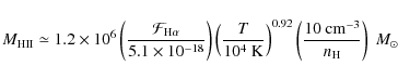
The mass of hot gas, within the equivalent volume
![]() associated with the aperture
associated with the aperture ![]() ,
is derived from the X-ray luminosity and the temperature
,
is derived from the X-ray luminosity and the temperature ![]() :
:
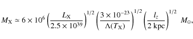
where
2.2.2 Postshock gas
The galaxy-wide collision creates a multi-phase interstellar medium where molecular and H II gas are embedded in a hot X-ray emitting plasma.
No postshock H I gas is detected in the shocked region where ![]() was observed. We derive an upper limit of 5
was observed. We derive an upper limit of 5 ![]()
![]() based on the lowest H I contour close to the shock. A two-temperature fit of the
based on the lowest H I contour close to the shock. A two-temperature fit of the ![]() excitation diagram gives T=185 K and T=675 K for the two gas components. Most of the gas mass is contained in the lower temperature component, which represents a mass of warm
excitation diagram gives T=185 K and T=675 K for the two gas components. Most of the gas mass is contained in the lower temperature component, which represents a mass of warm ![]() of 3
of 3 ![]()
![]() (Appleton et al. 2006) within the aperture
(Appleton et al. 2006) within the aperture ![]() .
Published CO observations do not constrain the total
.
Published CO observations do not constrain the total ![]() mass in the preshock and postshock gas. Given the uncertainties on the preshock gas masses, one cannot infer a precise mass of cold molecular gas.
mass in the preshock and postshock gas. Given the uncertainties on the preshock gas masses, one cannot infer a precise mass of cold molecular gas.
The mass of hot plasma is derived from the O'Sullivan et al. (2008) Chandra observations in the region observed by Spitzer. The absorption-corrected X-ray luminosity is 1.2 ![]() 1040 erg s-1 within the aperture
1040 erg s-1 within the aperture ![]() .
Using Eq. (2), this corresponds to a mass of 1.4
.
Using Eq. (2), this corresponds to a mass of 1.4 ![]()
![]() .
This is 2-3 times the mass of the preshock hot plasma. O'Sullivan et al. (2008) report variations of the average proton density in the range
.
This is 2-3 times the mass of the preshock hot plasma. O'Sullivan et al. (2008) report variations of the average proton density in the range
![]()
![]() 10-2 cm-3. The density peaks close to the area
10-2 cm-3. The density peaks close to the area ![]() .
We adopt a hot plasma density of
.
We adopt a hot plasma density of
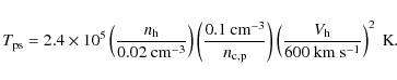
![]() cm-3 where
cm-3 where ![]() has been detected. This is in agreement with the value obtained by Trinchieri et al. (2005).
The postshock gas pressure is given by
has been detected. This is in agreement with the value obtained by Trinchieri et al. (2005).
The postshock gas pressure is given by
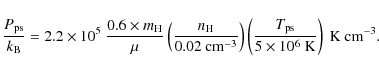 |
(3) |
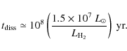
In the tenuous gas this pressure remains almost constant during the collision time scale since the plasma does not have the time to cool nor to expand significantly. The isobaric gas cooling time scale can be estimated as the ratio of the internal energy of the gas to the cooling rate:
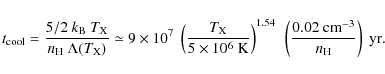
This cooling time is significantly longer than the age of the shock. In the right hand side of Eq. (4), we use the power-law fit of the Z=1 cooling efficiency given in Gnat & Sternberg (2007) (consistent with Sutherland & Dopita 1993). If the metallicity of the pre-shocked tidal filament was sub-solar, this would increase the cooling time of the gas still further. O'Sullivan et al. (2008) found a best fit to their X-ray spectrum for
The mass of the ionized H II gas is derived from the emission measure of H![]() observations:
observations:
 |
(5) |
where
2.3 Extinction and UV field
Xu et al. (2003) have interpreted their non-detection of the H![]() line as an indication of significant extinction (
line as an indication of significant extinction (
![]() ,
i.e.
,
i.e.
![]() ). However, more sensitive spectroscopy
). However, more sensitive spectroscopy![]() by Duc et al. (private communication) show that the H
by Duc et al. (private communication) show that the H![]() line is detected over the region observed with IRS at two velocity components (
line is detected over the region observed with IRS at two velocity components (
![]() and 6300 km s-1, corresponding to the intruder and the intra-group gas velocities). These observations show that the extinction is much higher (AV = 2.5) for the low-velocity gas component than for the high-velocity one. There are also large spatial variations of the extinction value for the intruder gas velocity close to this position, suggesting clumpiness of the gas within the disturbed spiral arm of NGC 7318b. An extinction of
AV=0.3-0.9 is derived from the Balmer decrement for the intra-group tidal tail velocity, with much lower spatial variation. After subtraction of the foreground galactic extinction (
AV = 0.24), this gives an SQ ridge extinction AV in the range 0.1-0.7.
and 6300 km s-1, corresponding to the intruder and the intra-group gas velocities). These observations show that the extinction is much higher (AV = 2.5) for the low-velocity gas component than for the high-velocity one. There are also large spatial variations of the extinction value for the intruder gas velocity close to this position, suggesting clumpiness of the gas within the disturbed spiral arm of NGC 7318b. An extinction of
AV=0.3-0.9 is derived from the Balmer decrement for the intra-group tidal tail velocity, with much lower spatial variation. After subtraction of the foreground galactic extinction (
AV = 0.24), this gives an SQ ridge extinction AV in the range 0.1-0.7.
A low extinction for the H2-rich, intra-group gas is also consistent with measured UV and far-IR dust surface brightness observations. Using the published value of FUV extinction (Xu et al. 2005) and the Weingartner & Draine (2001) extinction curve, we derive
AV = 0.29, which is in agreement with the new Balmer-decrement study. GALEX
observations show that the radiation field is
![]() in the shocked region, where G0 is the interstellar radiation field (ISRF) in Habing units
in the shocked region, where G0 is the interstellar radiation field (ISRF) in Habing units![]() . We obtain the higher value using the flux listed in Table 1 of Xu et al. (2005). This flux is measured over an area much larger than our aperture
. We obtain the higher value using the flux listed in Table 1 of Xu et al. (2005). This flux is measured over an area much larger than our aperture ![]() .
It provides an upper limit on the UV field in the shock because this area includes star forming regions in the spiral arm of NGC 7318b. ISO observations show a diffuse 100
.
It provides an upper limit on the UV field in the shock because this area includes star forming regions in the spiral arm of NGC 7318b. ISO observations show a diffuse 100 ![]() m emission at a 2.2 MJy sr-1 level in the shocked region (Xu et al. 2003). Using the Galactic model of Draine & Li (2007) for
G = 2 G0, the 100
m emission at a 2.2 MJy sr-1 level in the shocked region (Xu et al. 2003). Using the Galactic model of Draine & Li (2007) for
G = 2 G0, the 100 ![]() m FIR brightness corresponds to a gas column density of 1.5
m FIR brightness corresponds to a gas column density of 1.5 ![]() 1020 cm-2. For G = G0, we obtain
1020 cm-2. For G = G0, we obtain
![]()
![]() 1020 cm-2, which corresponds to
AV = 0.18 for the Solar neighbourhood value of the
1020 cm-2, which corresponds to
AV = 0.18 for the Solar neighbourhood value of the
![]() ratio. Since this value is low, no extinction correction is applied.
ratio. Since this value is low, no extinction correction is applied.
2.4 Energy reservoirs
The bulk kinetic energy of the pre- and postshock gas are the dominant terms of the energy budget of the SQ collision (Table 1). Assuming that the preshock H I mass is moving at
![]() km s-1 in the center of mass rest frame, the preshock gas bulk kinetic energy is 1-3
km s-1 in the center of mass rest frame, the preshock gas bulk kinetic energy is 1-3 ![]() 1056 erg. Note that this is a lower limit since a possible contribution from preshock molecular gas is not included. The thermal energy of the X-ray plasma represents
1056 erg. Note that this is a lower limit since a possible contribution from preshock molecular gas is not included. The thermal energy of the X-ray plasma represents ![]() % of the preshock kinetic energy.
% of the preshock kinetic energy.
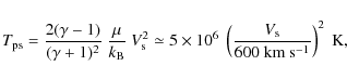
The shock distributes the preshock bulk kinetic energy into postshock thermal energy and bulk kinetic energy. The Spitzer IRS observations of SQ (Appleton et al. 2006) show that the 0-0 S(1) 17 ![]() m
m ![]() line is resolved with a width of 870
line is resolved with a width of 870 ![]() 60 km s-1 (FWHM), comparable to the collision velocity. We assume that the broad resolved line represents
60 km s-1 (FWHM), comparable to the collision velocity. We assume that the broad resolved line represents ![]() emission with a wide range of velocities, by analogy with the O I [6300 Å] emission seen in the same region by Xu et al. (2003) (see Appleton et al. 2006, for discussion). Then the results imply a substantial kinetic energy carried by the postshock gas. The kinetic energy of the
emission with a wide range of velocities, by analogy with the O I [6300 Å] emission seen in the same region by Xu et al. (2003) (see Appleton et al. 2006, for discussion). Then the results imply a substantial kinetic energy carried by the postshock gas. The kinetic energy of the ![]() gas is estimated by combining the line width with the warm
gas is estimated by combining the line width with the warm ![]() mass. This is a lower limit since there may be a significant mass of
mass. This is a lower limit since there may be a significant mass of ![]() too cold to be seen in emission. The
too cold to be seen in emission. The ![]() kinetic energy is more than 3 times the amount of thermal energy of the postshock hot plasma. This implies that most of the collision energy is not dissipated in the hot plasma, but a substantial amount is carried by the warm molecular gas.
kinetic energy is more than 3 times the amount of thermal energy of the postshock hot plasma. This implies that most of the collision energy is not dissipated in the hot plasma, but a substantial amount is carried by the warm molecular gas.
Radio synchrotron observations indicate that the postshock medium is magnetized. Assuming the equipartition of energy between cosmic rays and magnetic energy, the mean magnetic field strength in the SQ shocked region is
![]() G (Xu et al. 2003). The magnetic energy and thereby the cosmic ray energy contained in the volume
G (Xu et al. 2003). The magnetic energy and thereby the cosmic ray energy contained in the volume
![]() is
is
![]()
![]() 1054 erg. This energy is much lower than the bulk
kinetic energy of the
1054 erg. This energy is much lower than the bulk
kinetic energy of the ![]() gas.
gas.
Thus, the dominant postshock energy reservoir is the bulk kinetic energy of the molecular gas. We thus propose that the observed ![]() emission is powered by the dissipation of this kinetic energy. The ratio between the kinetic energy of the warm H2 gas in the center of mass frame and the
emission is powered by the dissipation of this kinetic energy. The ratio between the kinetic energy of the warm H2 gas in the center of mass frame and the ![]() luminosity is:
luminosity is:
 |
(6) |
The
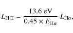
The line emission of the ionized gas could also contribute to the dissipation of energy.
We estimate the total luminosity of the postshock H II gas from the H![]() luminosity (Heckman et al. 1989):
luminosity (Heckman et al. 1989):
 |
(7) |
where
3 Why is H
present in the postshock gas?
Observations show that the pre-collision medium is inhomogeneous. The gas in the SQ group halo is observed to be structured with H I clouds and possibly ![]() clouds embedded in a teneous, hot, intercloud plasma (Sect. 2.1). On the intruder side, the galaxy interstellar medium is also expected to be multiphase. We consider a large-scale collision between two flows of multiphase dusty gas (Fig. 1). In this section we quantify
clouds embedded in a teneous, hot, intercloud plasma (Sect. 2.1). On the intruder side, the galaxy interstellar medium is also expected to be multiphase. We consider a large-scale collision between two flows of multiphase dusty gas (Fig. 1). In this section we quantify ![]() formation within this context. The details of the microphysics calculations of the dust evolution, gas cooling and
formation within this context. The details of the microphysics calculations of the dust evolution, gas cooling and ![]() formation are given in Appendices A-C.
formation are given in Appendices A-C.
3.1 Collision between two dusty multiphase gas flows
This section introduces a schematic description of the collision that allows us to quantify the ![]() formation timescale. The collision drives two high-velocity large-scale shocks that propagate through the teneous volume filling plasma, both into the tidal arm and into the intruder.
The rise in the intercloud pressure drives slower shocks into the clouds (e.g. McKee & Cowie 1975). The velocity of the transmitted shock into the clouds,
formation timescale. The collision drives two high-velocity large-scale shocks that propagate through the teneous volume filling plasma, both into the tidal arm and into the intruder.
The rise in the intercloud pressure drives slower shocks into the clouds (e.g. McKee & Cowie 1975). The velocity of the transmitted shock into the clouds, ![]() ,
is of the order of
,
is of the order of
![]() ,
where
,
where ![]() is the shock velocity in the hot intercloud medium, and
is the shock velocity in the hot intercloud medium, and ![]() and
and
![]() are the densities of the cloud and intercloud medium
are the densities of the cloud and intercloud medium![]() , respectively. Each cloud density corresponds to a shock velocity.
, respectively. Each cloud density corresponds to a shock velocity.
The galaxy collision generates a range of shock velocities and postshock gas temperatures. The state of the postshock gas is related to the preshock gas density. Schematically, low density (
![]() cm-3) gas is shocked at high speed (
cm-3) gas is shocked at high speed (![]() km s-1) and accounts for the X-ray emission. The postshock plasma did not have time to cool down significantly and form molecular gas since the collision was initiated. H I gas (
km s-1) and accounts for the X-ray emission. The postshock plasma did not have time to cool down significantly and form molecular gas since the collision was initiated. H I gas (
![]()
![]() 10-2) is heated to lower (
10-2) is heated to lower (![]() K) temperatures. This gas has time to cool. Since
K) temperatures. This gas has time to cool. Since ![]() forms on dust grains, dust survival is an essential element of our scenario (see Appendix A). The gas pressure is too high for warm neutral H I to be in thermal equilibrium. Therefore, the clouds cool to the temperatures of the cold neutral medium and become molecular.
forms on dust grains, dust survival is an essential element of our scenario (see Appendix A). The gas pressure is too high for warm neutral H I to be in thermal equilibrium. Therefore, the clouds cool to the temperatures of the cold neutral medium and become molecular.
The time dependence of both the gas temperature and the dust-to-gas mass ratio, starting from gas at an initial postshock temperature
![]() ,
has been calculated. We assume a galactic dust-to-gas ratio, a solar metallicity and equilibrium ionization. In the calculations, the thermal gas pressure is constant. As the gas cools, it condenses. Below
,
has been calculated. We assume a galactic dust-to-gas ratio, a solar metallicity and equilibrium ionization. In the calculations, the thermal gas pressure is constant. As the gas cools, it condenses. Below
![]() K, the H II gas recombines, cools through optical line emission, and becomes molecular. The gas and chemistry network code (Appendix C) follows the time evolution of the gas that recombines. The effect of the magnetic field on the compression of the gas has been neglected in the calculations and we assume a constant thermal gas pressure.
K, the H II gas recombines, cools through optical line emission, and becomes molecular. The gas and chemistry network code (Appendix C) follows the time evolution of the gas that recombines. The effect of the magnetic field on the compression of the gas has been neglected in the calculations and we assume a constant thermal gas pressure.
Under the usual flux-freezing ideas, the magnetic field strength should increase with volume density and limit the compression factor. However, observations show that the magnetic field in the cold neutral medium (CNM) is comparable to that measured in lower density, warm ISM components (Heiles & Troland 2005). 3D MHD numerical simulations of the supernovae-driven turbulence in the ISM also show that gas compression can occur over many orders of magnitude, without increasing the magnetic pressure (e.g. Mac Low et al. 2005; de Avillez & Breitschwerdt 2005b). The reason is that the lower density (
![]() cm-3) gas is magnetically sub-critical and mainly flows along the magnetic field lines without compressing the magnetic flux. The magnetic field intensity increases within gravitationally bound structures at higher gas densities (
cm-3) gas is magnetically sub-critical and mainly flows along the magnetic field lines without compressing the magnetic flux. The magnetic field intensity increases within gravitationally bound structures at higher gas densities (
![]() cm-3 (e.g. Hennebelle et al. 2008). This result is in agreement with observations of the magnetic field intensity in molecular clouds by Crutcher (1999) and Crutcher et al. (2003).
cm-3 (e.g. Hennebelle et al. 2008). This result is in agreement with observations of the magnetic field intensity in molecular clouds by Crutcher (1999) and Crutcher et al. (2003).
3.2 Gas cooling, dust destruction and H2 formation timescales
The physical state of the post-shock gas depends on the shock age, the gas cooling, the dust destruction, and the ![]() formation timescales. These relevant timescales are plotted as a function of the postshock temperature in Fig. 2. Given a shock velocity
formation timescales. These relevant timescales are plotted as a function of the postshock temperature in Fig. 2. Given a shock velocity ![]() in the low-density plasma, each value of the postshock temperature
in the low-density plasma, each value of the postshock temperature
![]() corresponds to a cloud preshock density
corresponds to a cloud preshock density
![]() :
:
 |
(8) |
Dust destruction is included in the calculation of the H2 formation timescale. The H2 formation timescale is defined as the time when the H2 fractional abundance reaches 90% of its final (end of cooling) value, including the gas cooling time from the postshock temperature. The dust destruction timescale is defined as the time when 90% of the dust mass is destroyed and returned to the gas. At T < 106 K, this timescale rises steeply because the dust sputtering rate drops (see Appendix A for details). The dust destruction timescale increases towards higher temperatures because, for a fixed pressure, the density decreases.
The present state of the multiphase postshock gas is set by the relative values of the three timescales at the SQ collision age, indicated with the horizontal dashed line and marked with an arrow. The ordering of the timescales depends on the preshock density and postshock gas temperature. By comparing these timescales one can define three gas phases, marked by blue, grey and red thick lines in Fig. 2.
- 1.
- The molecular phase: for

 105 K, the dust destruction timescale is longer than the collision age and the
  formation timescale is shorter. This gas keeps a significant fraction of its initial dust content and becomes
(blue thick line).
formation timescale is shorter. This gas keeps a significant fraction of its initial dust content and becomes
(blue thick line).
- 2.
- Atomic H I and ionized H II gas phase: for intermediate temperatures (8
 106 K), the gas has time to cool down but loses its dust content. The formation timescale is longer than the collision age. This phase is indicated with the grey thick line.
- 3.
- X-ray emitting plasma: at high temperatures (
 106 K), the postshock gas is dust-free and hot. This is the X-ray emitting plasma indicated by the red thick line.
In Fig. 2 it is assumed that, during the gas cooling, the molecular gas is in pressure equilibrium with the hot, volume filling gas. The gas pressure is set to the measured average thermal pressure of the hot plasma (HIM). Theoretical studies and numerical simulations show that the probability distribution function of the density in a supersonically turbulent isothermal gas is lognormal, with a dispersion which increases with the Mach number (Padoan et al. 1997; Mac Low et al. 2005; Passot & Vázquez-Semadeni 1998; Vazquez-Semadeni 1994). Based on these studies, the SQ postshock pressure in the turbulent cloud phase is likely to be widely distributed around the postshock pressure in the HIM (2 ![]() 105 K cm-3). The H2 formation timescale would be longer in the low pressure regions and shorter in high pressure regions.
105 K cm-3). The H2 formation timescale would be longer in the low pressure regions and shorter in high pressure regions.
To quantify this statement, we run a grid of isobaric cooling models for different gas thermal pressures. Figure 3 shows the gas cooling time and the ![]() formation timescale as a function of the gas thermal pressure. A Solar Neighborhood value of the dust-to-gas ratio is assumed. The
formation timescale as a function of the gas thermal pressure. A Solar Neighborhood value of the dust-to-gas ratio is assumed. The ![]() formation time scale roughly scales as the inverse of the gas density at 104 K and can be fitted by the following power-law:
formation time scale roughly scales as the inverse of the gas density at 104 K and can be fitted by the following power-law:
![\begin{displaymath}%
t_{\rm H_2}~{\rm [yr]} \simeq 7 \times 10^{5} ~ f_{\rm dust...
...{2 \times 10^{5}~{\rm [K~cm^{-3}]}}{P_{\rm th}}\right)^{0.95},
\end{displaymath}](/articles/aa/full_html/2009/29/aa11263-08/img111.png)
where
Figure 3 shows that for a wide range of gas thermal pressures (>3 ![]() 104 K cm-3, i.e.
104 K cm-3, i.e.
![]() ),
), ![]() can form within less than the collision age (5
can form within less than the collision age (5 ![]() 106 yrs). Numerical simulations of supernovae-driven turbulence in the ISM show that this condition applies to a dominant fraction of the gas mass (see Fig. 10 of Mac Low et al. 2005). Numerical studies by Glover & Mac Low (2007) show that the pressure variations induced by the turbulence globally reduce the time required to form large quantities of H2 within the Galactic CNM.
106 yrs). Numerical simulations of supernovae-driven turbulence in the ISM show that this condition applies to a dominant fraction of the gas mass (see Fig. 10 of Mac Low et al. 2005). Numerical studies by Glover & Mac Low (2007) show that the pressure variations induced by the turbulence globally reduce the time required to form large quantities of H2 within the Galactic CNM.
![\begin{figure}
\par\includegraphics[angle=90,width=8.5cm,clip]{11263fg3.eps}
\end{figure}](/articles/aa/full_html/2009/29/aa11263-08/img116.png) |
Figure 3:
Cooling and H2 formation timescales for ionized gas at 104 K as a function of the gas density and pressure (top axis). The grey horizontal bar indicates the SQ collision age, and the blue vertical bar shows the gas thermal pressure at which the |
3.3 Cloud crushing and fragmentation timescales
In Sect. 3.2, the microphysics of the gas has been quantified, ignoring the fragmentation of clouds by thermal, Rayleigh-Taylor and Kelvin-Helmholtz instabilities. In this section, we introduce the dynamical timescales associated with the fragmentation of clouds and compare them with the ![]() formation timescale.
formation timescale.
3.3.1 Fragmentation
When a cloud is overtaken by a strong shock wave, a flow of background gas establishes around it, and the cloud interacts with the low-density gas that is moving relative to it (see Fig. 1). The dynamical evolution of such a cloud has been described in many papers (e.g. Mac Low et al. 1994; Klein et al. 1994). Numerical simulations show that this interaction triggers clouds fragmentation. The shock compresses the cloud on a crushing time
![]() ,
where
,
where ![]() is the shock velocity in the cloud and
is the shock velocity in the cloud and ![]() its characteristic preshock size. The shocked cloud is subject to both Rayleigh-Taylor and Kelvin-Helmholtz instabilities.
its characteristic preshock size. The shocked cloud is subject to both Rayleigh-Taylor and Kelvin-Helmholtz instabilities.
Gas cooling introduces an additional fragmentation mechanism because the cooling gas is thermally unstable at temperatures smaller than
![]() K. The thermal instability generates complex inhomogeneous structures, dense regions that cool and low density voids (Audit & Hennebelle 2005; Sutherland et al. 2003). This fragmentation occurs on the gas cooling timescale. In most numerical simulations, the thermal instability is ignored because simplifying assumptions are made on the equation of state of the gas (adiabatic, isothermal or polytropic evolution).
K. The thermal instability generates complex inhomogeneous structures, dense regions that cool and low density voids (Audit & Hennebelle 2005; Sutherland et al. 2003). This fragmentation occurs on the gas cooling timescale. In most numerical simulations, the thermal instability is ignored because simplifying assumptions are made on the equation of state of the gas (adiabatic, isothermal or polytropic evolution).
In Fig. 4, the ![]() formation and gas cooling timescales are compared to the crushing time and collision age, as a function of the initial density and size of the cloud. The pressure of the clouds is 2
formation and gas cooling timescales are compared to the crushing time and collision age, as a function of the initial density and size of the cloud. The pressure of the clouds is 2 ![]() 105 K cm-3. The red zone indicates where the
105 K cm-3. The red zone indicates where the ![]() formation timescale is longer than the SQ collision age. In this domain, clouds do not have time to form
formation timescale is longer than the SQ collision age. In this domain, clouds do not have time to form ![]() .
The blue hatched zone defines the range of sizes and densities of the clouds which become molecular within 5
.
The blue hatched zone defines the range of sizes and densities of the clouds which become molecular within 5 ![]() 106 yr. In this zone, the crushing time is longer than the cooling time. Gas fragments by thermal instability as the shock moves into the cloud.
106 yr. In this zone, the crushing time is longer than the cooling time. Gas fragments by thermal instability as the shock moves into the cloud. ![]() forms before the shock has crossed the cloud and therefore before Rayleigh-Taylor and Kelvin-Helmholtz instabilities start to develop. The black dashed line is where the cloud crushing timescale equals the SQ collision age (5
forms before the shock has crossed the cloud and therefore before Rayleigh-Taylor and Kelvin-Helmholtz instabilities start to develop. The black dashed line is where the cloud crushing timescale equals the SQ collision age (5 ![]() 106 yr). To the right of this line, the clouds have not been completely overtaken and compressed by the transmitted shock.
106 yr). To the right of this line, the clouds have not been completely overtaken and compressed by the transmitted shock.
Preshock Giant Molecular Clouds (hereafter GMCs) of size ![]() pc and mean density
pc and mean density ![]()
![]() 102 cm-3, like those observed in spiral galaxies, fall within the yellow zone in Fig. 4. The bottom boundary corresponds to the density at which the free-fall time equals the age of the SQ collision. For densities higher than this limit, the free-fall time is shorter than the SQ collision age. The left boundary of this area is the maximum cloud size set by the Bonnor-Ebert criterion for a pressure of 2
102 cm-3, like those observed in spiral galaxies, fall within the yellow zone in Fig. 4. The bottom boundary corresponds to the density at which the free-fall time equals the age of the SQ collision. For densities higher than this limit, the free-fall time is shorter than the SQ collision age. The left boundary of this area is the maximum cloud size set by the Bonnor-Ebert criterion for a pressure of 2 ![]() 105 K cm-3. Clouds with larger sizes are gravitationally unstable. Such clouds are expected to form stars.
105 K cm-3. Clouds with larger sizes are gravitationally unstable. Such clouds are expected to form stars.
A natural consequence of pre-existing GMCs would be that the shock would trigger their rapid collapse and star formation should rapidly follow (e.g. Jog & Solomon 1992). The absence (or weakness) of these tracers in the region of the main shock (Xu et al. 2003) suggests that fragments of preshock GMCs disrupted by star formation are not a major source of the observed postshock ![]() gas. However, it is possible that some of the gas in the intruder did contain pre-existing molecular material. The star formation regions seen to the North and South of the ridge are consistent with this hypothesis.
gas. However, it is possible that some of the gas in the intruder did contain pre-existing molecular material. The star formation regions seen to the North and South of the ridge are consistent with this hypothesis.
3.3.2 Survival of the fragments
The breakup of clouds can lead to mixing of cloud gas with the hot background plasma (Nakamura et al. 2006) and thereby raises the question of whether the cloud fragments survive long enough for H2 to form. Fragments evaporate into the background gas when their size is such that
the heat conduction rate overtakes the cooling rate. The survival of the fragments thus depends on their ability to cool (Mellema et al. 2002; Fragile et al. 2004). Gas condensation and ![]() formation are both expected to have a stabilizing effect on the cloud fragments, because they increase the gas cooling power (Le Bourlot et al. 1999).
formation are both expected to have a stabilizing effect on the cloud fragments, because they increase the gas cooling power (Le Bourlot et al. 1999).
So far, no simulations include the full range of densities and spatial scales and the detailed micro-physics that are involved in the cloud fragmentation and eventual mixing with the background gas. Slavin (2006) reports an analytical estimate of the evaporation time scale of tiny H I clouds embedded in warm and hot gas of several million years. This timescale is long enough for H2 to form within the lifetime of the gas fragments.
![\begin{figure}
\par\includegraphics[angle=90,width=12cm,clip]{11263fg5.eps}
\end{figure}](/articles/aa/full_html/2009/29/aa11263-08/img124.png) |
Figure 5:
|
Table 2: Overview of the emission of the SQ postshock gas, from observations and model predictionsa. The models are the same as those used in Fig. 5.
4 H
excitation
This section addresses the question of ![]() excitation. The models (Sect. 4.1) and the results (Sect. 4.2) are presented.
excitation. The models (Sect. 4.1) and the results (Sect. 4.2) are presented.
4.1 Modeling the dissipation of turbulent kinetic energy by MHD shocks
Given that the dominant postshock energy reservoir is the bulk kinetic energy of the ![]() gas (Sect. 2.4), the
gas (Sect. 2.4), the ![]() emission is assumed to be powered by the dissipation of turbulent kinetic energy into molecular gas. Radio synchrotron observations indicate that the postshock medium is magnetized (Sect. 2.4). In this context, the dissipation of mechanical energy within molecular gas is modeled by non-dissociative MHD shocks. In the absence of a magnetic field, shocks are rapidly dissociative and much of the cooling of the shocked gas occurs through atomic, rather than H2, line emission. We quantify the required gas densities and shock velocities to account for the
emission is assumed to be powered by the dissipation of turbulent kinetic energy into molecular gas. Radio synchrotron observations indicate that the postshock medium is magnetized (Sect. 2.4). In this context, the dissipation of mechanical energy within molecular gas is modeled by non-dissociative MHD shocks. In the absence of a magnetic field, shocks are rapidly dissociative and much of the cooling of the shocked gas occurs through atomic, rather than H2, line emission. We quantify the required gas densities and shock velocities to account for the ![]() excitation diagram.
excitation diagram.
The ![]() emission induced by low velocity shocks is calculated using an updated version of the shock model of Flower & Pineau des Forêts (2003). In these models, we assume a standard value for the cosmic ray ionization rate of
emission induced by low velocity shocks is calculated using an updated version of the shock model of Flower & Pineau des Forêts (2003). In these models, we assume a standard value for the cosmic ray ionization rate of ![]()
![]() 10-17 s-1. In its initial state,
the gas is molecular and cold (
10-17 s-1. In its initial state,
the gas is molecular and cold (![]() K), with molecular abundances resulting from the output of our model for the isobaric cooling (Sect. C.2 and Fig. C.2). A grid of shock models has been computed for shock velocities from 3 to 40 km s-1 with steps of 1 km s-1, two values of the initial
K), with molecular abundances resulting from the output of our model for the isobaric cooling (Sect. C.2 and Fig. C.2). A grid of shock models has been computed for shock velocities from 3 to 40 km s-1 with steps of 1 km s-1, two values of the initial ![]() ortho to para ratio (3 and 10-2), and 3 different preshock densities (
ortho to para ratio (3 and 10-2), and 3 different preshock densities (
![]() ,
103, and 104 cm-3). We adopt the scaling of the initial magnetic strength with
the gas density,
,
103, and 104 cm-3). We adopt the scaling of the initial magnetic strength with
the gas density,
![]() (Hennebelle et al. 2008; Crutcher 1999). In our models, b=1.
(Hennebelle et al. 2008; Crutcher 1999). In our models, b=1.
4.2 Results: contribution of MHD shocks to the H2 excitation
Results are presented in terms of an H2 excitation diagram, where the logarithm of the column densities
![]() ,
divided by the statistical weight
,
divided by the statistical weight ![]() ,
are plotted versus the energy of the corresponding level. The excitation diagrams are calculated for a gas temperature of 50 K, since the molecular gas colder than 50 K does not contribute to the H2 emission. Figure 5 shows the
,
are plotted versus the energy of the corresponding level. The excitation diagrams are calculated for a gas temperature of 50 K, since the molecular gas colder than 50 K does not contribute to the H2 emission. Figure 5 shows the ![]() excitation diagram for both observations and model. The SQ data from Appleton et al. (2006) is indicated with
excitation diagram for both observations and model. The SQ data from Appleton et al. (2006) is indicated with ![]() error bars. The
error bars. The ![]() line fluxes have been converted to mean column densities within our area
line fluxes have been converted to mean column densities within our area ![]() .
.
The observed rotational diagram is curved, suggesting that the H2-emitting gas is a mixture of components at different temperatures. The data cannot be fitted with a single shock. At least two different shock velocities are needed. A least-squares fit of the observed ![]() line fluxes to a linear combination of 2 MHD shocks at different velocities
line fluxes to a linear combination of 2 MHD shocks at different velocities
![]() and
and
![]() has been performed. For a preshock density of 104 cm-3, the best fit is obtained for a combination of 5 and 20 km s-1 shocks with an initial value of the ortho to para ratio of 3 (Fig. 5 and Table 2). Note that no satisfactory fit could be obtained with the low value of the initial H2 ortho-to-para ratio. The contributions of the 5 (green dashed line) and 20 km s-1 (orange dashed line) shocks to the total column densities are also plotted. Qualitatively, the 5 km s-1 component dominates the contribution to the column densities of the upper levels of S(0) and S(1) lines. The 20 km s-1 component has a major contribution for the upper levels of S(3) to S(5). For S(2), the 2 contributions are comparable. The red line shows the weighted sum of the two shock components (best fit). The warm H2 pressure
has been performed. For a preshock density of 104 cm-3, the best fit is obtained for a combination of 5 and 20 km s-1 shocks with an initial value of the ortho to para ratio of 3 (Fig. 5 and Table 2). Note that no satisfactory fit could be obtained with the low value of the initial H2 ortho-to-para ratio. The contributions of the 5 (green dashed line) and 20 km s-1 (orange dashed line) shocks to the total column densities are also plotted. Qualitatively, the 5 km s-1 component dominates the contribution to the column densities of the upper levels of S(0) and S(1) lines. The 20 km s-1 component has a major contribution for the upper levels of S(3) to S(5). For S(2), the 2 contributions are comparable. The red line shows the weighted sum of the two shock components (best fit). The warm H2 pressure
![]() in the two shocks is 4.5
in the two shocks is 4.5 ![]() 107 K cm-3 (respectively 5.6
107 K cm-3 (respectively 5.6 ![]() 108 K cm-3) for the 5 km s-1 (resp. 20 km s-1) shock.
108 K cm-3) for the 5 km s-1 (resp. 20 km s-1) shock.
Our grid of models shows that this solution is not unique. If one decreases the density to 103 cm-3, we find that one can fit the observations with a combination of MHD shocks (at 9 and 35 km s-1). If one decreases the density to 102 cm-3, the rotational ![]() excitation cannot be fitted satisfactorily. At such low densities, MHD shocks fail to reproduce the S(3) and S(5) lines because the critical densities for rotational H2 excitation increase steeply with the J rotational quantum number (Le Bourlot et al. 1999). Both warm and dense (i.e. high pressure) gas is needed to account for emission from the higher J levels.
excitation cannot be fitted satisfactorily. At such low densities, MHD shocks fail to reproduce the S(3) and S(5) lines because the critical densities for rotational H2 excitation increase steeply with the J rotational quantum number (Le Bourlot et al. 1999). Both warm and dense (i.e. high pressure) gas is needed to account for emission from the higher J levels.
The data fit gives an estimate of the shock velocities required to account for the H2 excitation. The velocities are remarkably low compared to the SQ collision velocity. The fact that energy dissipation occurs over this low velocity range is an essential key to account for the importance of H2 cooling. High velocity shocks would dissociate H2 molecules.
![\begin{figure}
\par\includegraphics[width=8.8cm,clip]{11263fg6.eps}
\end{figure}](/articles/aa/full_html/2009/29/aa11263-08/img149.png) |
Figure 6:
Schematic view of the evolutionary cycle of the gas proposed in our interpretation of optical and H2 observations of Stephan's Quintet. Arrows represent the mass flows between the H II, warm H I, warm and cold H2 gas components. They are numbered for clarity (see text). The dynamical interaction between gas phases drives the cycle. The values of the mass flows and associated timescales are derived from the
|
5 The cycling of gas across ISM phases
An evolutionary picture of the inhomogeneous postshock gas emerges from our interpretation of the data. The powerful ![]() emission is part of a broader astrophysical context, including optical and X-ray emission, which can be understood in terms of mass exchange between gas phases. A schematic diagram of the evolutionary picture of the postshock gas is presented in Fig. 6. It illustrates the cycle of mass between the ISM phases that we detail here. This view of the SQ postshock gas introduces a physical framework that may apply to H2 luminous galaxies in general.
emission is part of a broader astrophysical context, including optical and X-ray emission, which can be understood in terms of mass exchange between gas phases. A schematic diagram of the evolutionary picture of the postshock gas is presented in Fig. 6. It illustrates the cycle of mass between the ISM phases that we detail here. This view of the SQ postshock gas introduces a physical framework that may apply to H2 luminous galaxies in general.
5.1 Mass flows
The ![]() gas luminosity is proportional to the mass of gas that cools per unit time, the so-called mass flow. We compute the mass flow associated with one given shock, dividing the postshock column density, associated with the gas cooling to a temperature of 50 K, by the cooling time needed to reach this temperature. Gas cooler than 50 K does not contribute to the
gas luminosity is proportional to the mass of gas that cools per unit time, the so-called mass flow. We compute the mass flow associated with one given shock, dividing the postshock column density, associated with the gas cooling to a temperature of 50 K, by the cooling time needed to reach this temperature. Gas cooler than 50 K does not contribute to the ![]() emission.
emission.
The two-component shock model has been used to deduce the mass flows needed to fit the data.
The cooling timescale (down to 50 K) is set by the lowest shock velocity component. For a shock velocity of 5 km s-1, the cooling time is ![]()
![]() 104 yr. This gives a total mass flow required to fit the
104 yr. This gives a total mass flow required to fit the ![]() emission of
emission of
![]()
![]()
![]() yr-1. For comparison, for the 20 km s-1 shock, the cooling time down to 50 K is
yr-1. For comparison, for the 20 km s-1 shock, the cooling time down to 50 K is ![]()
![]() 103 yr and the associated mass flow is
103 yr and the associated mass flow is
![]() yr-1.
yr-1.
These mass flows are compared to the mass flow of recombining gas that can be estimated from the H![]() luminosity
luminosity
![]() :
:
| (10) |
where
The H2 emission integrated over the isobaric cooling sequence is calculated. The blue dashed curve of Fig. 5 corresponds to the model results for a mass flow of
![]() and a pressure
and a pressure
![]()
![]() 105 K cm-3. The model results do not depend much on the pressure. The model reproduces well the shape of the observed excitation diagram, but the emission is a factor
105 K cm-3. The model results do not depend much on the pressure. The model reproduces well the shape of the observed excitation diagram, but the emission is a factor ![]() below the observations. The model also fails to reproduce the [O I] 6300 Å line emission by a factor of 7. Therefore, the cooling of the warm H I gas produced by H II recombination cannot reproduce the observed
below the observations. The model also fails to reproduce the [O I] 6300 Å line emission by a factor of 7. Therefore, the cooling of the warm H I gas produced by H II recombination cannot reproduce the observed ![]() emission nor the [O I] 6300 Å line emission. A larger amount of energy needs to be dissipated within the molecular gas to account for the
emission nor the [O I] 6300 Å line emission. A larger amount of energy needs to be dissipated within the molecular gas to account for the ![]() emission. This is why the total mass flow associated with the 2-component MHD shocks is much larger than the mass flow of recombining gas.
emission. This is why the total mass flow associated with the 2-component MHD shocks is much larger than the mass flow of recombining gas.
5.2 The mass cycle
This section describes the mass cycle of Fig. 6. Black and red arrows represent the mass flows between the H II, warm H I, warm and cold H2 gas components of the postshock gas. The large red arrow to the left symbolizes the relative motion between the warm and cold gas and the surrounding plasma. Each of the black arrows is labeled with its main associated process: gas recombination and ionization (double arrow number 1), H2 formation (2) and H2 cooling (3). The values of the mass flows and the associated timescales are derived from observations and our model calculations (Sect. 5.1 and Table 2).
A continuous cycle through gas components is excluded by the increasing mass flow needed to account for the
![]() ,
O I, and
,
O I, and ![]() luminosities. Heating of the cold H2 gas towards warmer gas states (red arrows) must occur. The postshock molecular cloud fragments are likely to experience a distribution of shock velocities. Arrow number 4 represents the low velocity MHD shock excitation of H2 gas described in Sect. 4.1. A cyclic mass exchange between the cold molecular gas and the warm gas phases is also supported by the high value of the
luminosities. Heating of the cold H2 gas towards warmer gas states (red arrows) must occur. The postshock molecular cloud fragments are likely to experience a distribution of shock velocities. Arrow number 4 represents the low velocity MHD shock excitation of H2 gas described in Sect. 4.1. A cyclic mass exchange between the cold molecular gas and the warm gas phases is also supported by the high value of the ![]() ortho to para ratio (Sect. 4.1). More energetic shocks may dissociate the molecular gas (arrows number 5). They are necessary to account for the low O I luminosity.
Even more energetic shocks can ionize the molecular gas (arrow number 6). This would bring cold
ortho to para ratio (Sect. 4.1). More energetic shocks may dissociate the molecular gas (arrows number 5). They are necessary to account for the low O I luminosity.
Even more energetic shocks can ionize the molecular gas (arrow number 6). This would bring cold ![]() directly into the H II component. Such shocks have been proposed as the ionization source of the clouds in the Magellanic Stream by Bland-Hawthorn et al. (2007) based on hydrodynamic simulations of their interaction with the Galactic halo plasma.
directly into the H II component. Such shocks have been proposed as the ionization source of the clouds in the Magellanic Stream by Bland-Hawthorn et al. (2007) based on hydrodynamic simulations of their interaction with the Galactic halo plasma.
Turbulent mixing of hot, warm and cold gas is an alternative route to mass input of H II gas. Turbulent mixing layers have been described by Begelman & Fabian (1990) and Slavin et al. (1993). They result from the shredding of the cloud gas into fragments that become too small to survive evaporation due to heat conduction. It is represented by the thin blue and green arrows to the left of our cartoon. Turbulent mixing produces intermediate temperature gas that is thermally unstable. This gas cools back to produce H II gas that enters the cycle (thin green arrow). It is relevant for our scenario to note that cold gas in mixing layers preserves its dust content. It is only heated to a few 105 K, well below temperatures for which thermal sputtering becomes effective. Further, metals from the dust-free hot plasma brought to cool are expected to accrete on dust when gas cools and condenses. Far-UV O VI line observations are needed to quantify the mass flow rate through this path of the cycle and thereby the relative importance of photoionization (arrow 1), ionizing shocks (arrow 6), and turbulent mixing with hot gas
in sustaining the observed rate (
![]() yr-1) of recombining H II gas.
yr-1) of recombining H II gas.
Within this dynamical picture of the postshock gas, cold molecular gas is not necessarily a mass sink. Molecular gas colder than 50 K does not contribute to the H2 emission. The mass accumulated in this cold H2 gas depends on the ratio between the timescale of mechanical energy dissipation (on which gas is excited by shocks through one of the red arrows 4-6) and the cooling timescale along the black arrow 3.
6 Why is H
a dominant coolant of the postshock gas?
This section sketches the energetics of the molecular gas in relation to its interaction with the background plasma. An efficient transfer of the bulk kinetic energy of the gas to turbulent motions of much lower velocities within molecular clouds is required to make H2 a dominant coolant of the postshock gas. We consider that the bulk kinetic energy of the clouds drives the gas cycling through the warm/cold H II, H I and H2 states of multiphase fragmentary clouds and feeds the cloud turbulence. This hypothesis is supported by the fact that the mechanical energy is the main energy reservoir (Sect. 2.4). The energetics of the gas are discussed within this framework.
6.1 Cloud dynamics and energy transfer
In the collision, the clouds do not share the same dynamics as the lower density intercloud gas. The clouds keep their preshock momentum and move at high velocity with respect to the background plasma. The kinetic energy recorded in the
![]() H2 line width is dominated by the bulk motion of the H2 clouds in the plasma rest frame. The turbulent velocities required within clouds to excite H2 have a much smaller amplitude (relative fragment velocities up to 20 km s-1). The cloud turbulence needs to be continuously sustained to balance energy dissipation. An efficient transfer of the bulk kinetic energy to low velocity turbulence of the molecular gas is required to make H2 a dominant coolant of the postshock gas. Dissipation within either the hot plasma or warm atomic gas, leading to radiation at X-ray or optical wavelengths that is not efficiently absorbed by the molecular gas, has to be minor.
H2 line width is dominated by the bulk motion of the H2 clouds in the plasma rest frame. The turbulent velocities required within clouds to excite H2 have a much smaller amplitude (relative fragment velocities up to 20 km s-1). The cloud turbulence needs to be continuously sustained to balance energy dissipation. An efficient transfer of the bulk kinetic energy to low velocity turbulence of the molecular gas is required to make H2 a dominant coolant of the postshock gas. Dissipation within either the hot plasma or warm atomic gas, leading to radiation at X-ray or optical wavelengths that is not efficiently absorbed by the molecular gas, has to be minor.
We are far from being able to describe how the energy transfer occurs. We can only make qualitative statements that would need to be quantified with numerical simulations in future studies. The cloud motion is subject to drag from the background flow (Murray & Lin 2004). This drag corresponds to an exchange of momentum and energy with the background plasma which drives turbulence into the clouds.
The fragmented, multiphase structure of the clouds is likely to be a main key of the energy transfer. The dynamical interaction with the background plasma flow generates relative velocities between cloud fragments because their acceleration depends on their mass and density. The relative motion between cloud fragments can lead to collisions, which results in the dissipation of kinetic energy (Sect. 4.1). This dissipation will occur preferentially in the molecular gas because it is the coldest component with the lowest sound speed. The magnetic field is likely to be important because it binds the cloud H2 fragments to the lower density cloud gas which is more easily entrained by the background plasma flow. The mass cycle between cloud gas states contributes to the energy transfer in two ways. (1) Gas cooling transfers the turbulent energy of the warm H II and H I to the H2 gas. (2) The thermal instability which occurs when the gas cools both from 106 K and from 104 K transfers a significant fraction of the gas thermal energy to turbulent kinetic energy. Numerical simulations (Audit & Hennebelle 2005; Sutherland et al. 2003) show that the thermal instability inhibits energy-loss through radiation from the warmer gas and feeds turbulence in the cooler gas. The turbulent velocities generated by the thermal instability are found to be commensurate with the sound speed in the warmer gas and are thus supersonic for the colder gas.
6.2 Gas energetics
The turbulent energy of the cloud and the dissipated power per H2 molecule may be written as
 |
(11) |
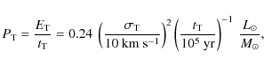 |
(12) |
where
If dissipation of turbulent energy powers the H2 emission, the energy dissipation rate must be at least equal to the power radiated by H2. Using the H2 emission and the warm H2 mass in Table 1, we estimate the luminosity to mass ratio of the warm H2 gas in SQ to be
![]() .
The dissipated power
.
The dissipated power ![]() may be somewhat larger if it powers the dissociative and ionizing shocks represented by the arrows 5 and 6 in Fig. 6.
This calculation implies a dissipation timescale of
may be somewhat larger if it powers the dissociative and ionizing shocks represented by the arrows 5 and 6 in Fig. 6.
This calculation implies a dissipation timescale of ![]()
![]() 104 yr which is not much higher than the cooling time of the lower excitation warm H2 gas that accounts for the S(0) and S(1) line emission (Sect. 5.1). Cold H2 gas would thus be heated by turbulent dissipation on timescales comparable to the gas cooling time. If this is correct, the cold molecular gas mass should not be much higher than the warm H2 mass inferred from the Spitzer observations. The turbulence dissipation timescale is more than three
orders of magnitude smaller than the ratio between the H2 gas bulk kinetic energy and H2 luminosity (Sect. 2.1). Thereby, the dissipation of the collision energy must involve a large (
104 yr which is not much higher than the cooling time of the lower excitation warm H2 gas that accounts for the S(0) and S(1) line emission (Sect. 5.1). Cold H2 gas would thus be heated by turbulent dissipation on timescales comparable to the gas cooling time. If this is correct, the cold molecular gas mass should not be much higher than the warm H2 mass inferred from the Spitzer observations. The turbulence dissipation timescale is more than three
orders of magnitude smaller than the ratio between the H2 gas bulk kinetic energy and H2 luminosity (Sect. 2.1). Thereby, the dissipation of the collision energy must involve a large (![]() )
number of cycles where H2 gas fragments are accelerated and dissipate their kinetic energy in shocks.
)
number of cycles where H2 gas fragments are accelerated and dissipate their kinetic energy in shocks.
7 Future tests of the model and open questions
In this section, we provide a few observational predictions of the model related to questions that remain open. For each point, we discuss which observations could test these predictions.
7.1 Dust emission
Dust is a key element in our scenario. It must be present in the postshock clouds for ![]() to form. Xu et al. (1999,2003) present results from infrared imaging observations carried out with the Infrared Space Observatory (ISO). Far-infrared (FIR) emission was detected in the shock region and Xu et al. (2003) proposed that it arises from large dust grains in the hot X-ray emitting plasma. Clearly, the Spitzer detection of molecular gas opens a new perpective on the origin of this emission. In our model, we expect that some of the thermal dust emission comes from the molecular gas. Outside the local UV enhancements associated with star formation seen in GALEX
to form. Xu et al. (1999,2003) present results from infrared imaging observations carried out with the Infrared Space Observatory (ISO). Far-infrared (FIR) emission was detected in the shock region and Xu et al. (2003) proposed that it arises from large dust grains in the hot X-ray emitting plasma. Clearly, the Spitzer detection of molecular gas opens a new perpective on the origin of this emission. In our model, we expect that some of the thermal dust emission comes from the molecular gas. Outside the local UV enhancements associated with star formation seen in GALEX![]() observations (Xu et al. 2005), dust emission should appear spatially correlated with the
observations (Xu et al. 2005), dust emission should appear spatially correlated with the ![]() emission. Given that the value of the radiation field in the shock is low (
emission. Given that the value of the radiation field in the shock is low (
![]() G0 Sect. 2.3), we expect rather faint dust emission in the SQ ridge. This accounts for the weakness of the Polycyclic Aromatic Hydrocarbons (PAH) features in the Spitzer spectra. Deep Spitzer imaging observations have been undertaken and will allow us to test this prediction. Moreover, observations with the Herschel Space Observatory will have the required angular resolution and sensitivity to detect the long wavelength emission of the dust in the SQ shock.
G0 Sect. 2.3), we expect rather faint dust emission in the SQ ridge. This accounts for the weakness of the Polycyclic Aromatic Hydrocarbons (PAH) features in the Spitzer spectra. Deep Spitzer imaging observations have been undertaken and will allow us to test this prediction. Moreover, observations with the Herschel Space Observatory will have the required angular resolution and sensitivity to detect the long wavelength emission of the dust in the SQ shock.
7.2 Mass budget
The Spitzer ![]() observations only trace the warm molecular gas (
observations only trace the warm molecular gas (![]() K). This warm gas could be physically connected to a more massive reservoir of cold
K). This warm gas could be physically connected to a more massive reservoir of cold ![]() gas. This is a major open question about the physical state of the molecular gas, as well as about the mass and energy budget. In a forthcoming paper, we will report the detection of CO(1-0) and (2-1) emision from cold molecular gas associated with the H
gas. This is a major open question about the physical state of the molecular gas, as well as about the mass and energy budget. In a forthcoming paper, we will report the detection of CO(1-0) and (2-1) emision from cold molecular gas associated with the H![]() emitting molecular gas. The physical state of the shocked gas is likely to be different to that of GMCs in galactic disks which are gravitationally bound. It is thus not clear that the standard CO emission to
emitting molecular gas. The physical state of the shocked gas is likely to be different to that of GMCs in galactic disks which are gravitationally bound. It is thus not clear that the standard CO emission to ![]() mass
conversion factor applies. Herschel observations of the dust emission will provide an estimate of the mass of cold gas, independent of the CO/
mass
conversion factor applies. Herschel observations of the dust emission will provide an estimate of the mass of cold gas, independent of the CO/![]() ratio.
ratio.
7.3 Shock energetics
Spitzer observations of the low-excitation ![]() rotational lines do not provide a complete budget of the kinetic energy dissipation. To constrain the present scenario, observations
of both higher and lower excitation lines are required. Rovibrational
rotational lines do not provide a complete budget of the kinetic energy dissipation. To constrain the present scenario, observations
of both higher and lower excitation lines are required. Rovibrational ![]() lines would probe dissipation in more energetic shocks than those inferred from the H2 pure rotational lines. If the molecular gas only experiences low-velocity MHD shocks, our model predicts a 1-0 S(1) line flux of 3.6
lines would probe dissipation in more energetic shocks than those inferred from the H2 pure rotational lines. If the molecular gas only experiences low-velocity MHD shocks, our model predicts a 1-0 S(1) line flux of 3.6 ![]() 10-19 W m-2 within the aperture
10-19 W m-2 within the aperture ![]() (Table 2). This is likely to be a strict lower limit since the dynamical interaction between the gas phases may well drive higher shock velocities (Sect. 3.1). Observations of the O I [63
(Table 2). This is likely to be a strict lower limit since the dynamical interaction between the gas phases may well drive higher shock velocities (Sect. 3.1). Observations of the O I [63 ![]() m] line would provide constraints on the physical state of colder molecular gas. The luminosity ratio of
m] line would provide constraints on the physical state of colder molecular gas. The luminosity ratio of ![]() rotational lines to O I depends on the shock velocity and the gas density. For the SQ ridge, the observed
rotational lines to O I depends on the shock velocity and the gas density. For the SQ ridge, the observed ![]() 0-0 S(1) line flux within the area
0-0 S(1) line flux within the area ![]() is 2
is 2 ![]() 10-17 W m-2, and our model predicts a
10-17 W m-2, and our model predicts a ![]() 0-0 S(1) to O I [63
0-0 S(1) to O I [63 ![]() m] luminosity ratio of 2.5. The Integral Field Spectrometer of the PACS
m] luminosity ratio of 2.5. The Integral Field Spectrometer of the PACS![]() instrument onboard the Herschel satellite should be able to detect the O I[63
instrument onboard the Herschel satellite should be able to detect the O I[63 ![]() m] line in one hour of integration. The spectral resolution of these observation will be a factor
m] line in one hour of integration. The spectral resolution of these observation will be a factor ![]() higher than Spitzer. The O I [63
higher than Spitzer. The O I [63 ![]() m] line profiles will allow us to compare the kinematics across the different temperatures of the gas. If the emission arises from multiphase clouds where warm and cold components are mixed down to small scales, their kinematics should be the same.
m] line profiles will allow us to compare the kinematics across the different temperatures of the gas. If the emission arises from multiphase clouds where warm and cold components are mixed down to small scales, their kinematics should be the same.
7.4 Star formation in the postshock gas
Many galaxy collisions and mergers are observed to trigger IR-luminous bursts of star formation.
However, the absence or weakness of spectroscopic signatures of photoionization (dust or ionized gas lines) in the center of the SQ ridge (Xu et al. 2003), where bright ![]() emission was detected by Spitzer, show that star formation does not occur in this region. Within the physical framework of dynamical interaction between gas phases described in Sects. 5 and 6, these observations suggest that most of the H2 emission arises from molecular fragments that are not massive enough or not long-lived enough to collapse. Star formation may also be quenched by continuous heating of the molecular gas and/or by the magnetic pressure if the dense cloud fragments are not magnetically supercritical (Sect. 3.1). Star-forming regions possibly associated with the galaxy collision are present away from the center of the shock (Lisenfeld et al. 2002; Xu et al. 1999,2003; Smith & Struck 2001; Gao & Xu 2000).
emission was detected by Spitzer, show that star formation does not occur in this region. Within the physical framework of dynamical interaction between gas phases described in Sects. 5 and 6, these observations suggest that most of the H2 emission arises from molecular fragments that are not massive enough or not long-lived enough to collapse. Star formation may also be quenched by continuous heating of the molecular gas and/or by the magnetic pressure if the dense cloud fragments are not magnetically supercritical (Sect. 3.1). Star-forming regions possibly associated with the galaxy collision are present away from the center of the shock (Lisenfeld et al. 2002; Xu et al. 1999,2003; Smith & Struck 2001; Gao & Xu 2000).
In our model, star formation may arise from the collapse of pre-existing GMCs (see Sect. 3.3). An alternative route to star formation may be the formation of gravitationally unstable postshock fragments. This second possibility has been quantified with numerical simulations that introduced the concept of turbulence-regulated star formation (Mac Low & Klessen 2004). Krumholz & McKee (2005) present an analytical description of the results of simulations, where the star formation rate depends on the Mach number of the turbulence within clouds and the ratio between their gravitational and turbulent kinetic energy. The star formation rate increases with the Mach number, but it is low even for high Mach numbers when the ratio between binding and turbulent energy is low. In the center of the SQ ridge, the star formation may be low because the average gas density is low (see Table 1), even if the amount of turbulent energy is high. The low gas density and large-scale dynamical context (high-velocity dispersion) does not favor the formation of gravitationnally bound molecular clouds, such as galactic GMCs.
8 Conclusions
Spitzer Space Telescope observations led to the surprising detection of H2 luminous
extragalactic sources whose mid-infrared spectra are dominated by molecular hydrogen line emission.
The absence or weakness of dust features or lines of ionized gas suggests the presence of large quantities of warm molecular gas with no or very little star formation. This work focuses on one of these H2 luminous galaxies: the Stephan's Quintet (SQ) galaxy-wide shock, created by the collision between an intruding galaxy and a tidal arm at a relative speed
![]() .
SQ observations place molecular gas in a new context where one has (1) to account for the presence of H2 in a galaxy halo; (2) to characterize its physical state and (3) to describe its role as a cooling agent of an energetic phase of galaxy interaction. The aim of the paper is to answer three main questions: (i) Why is there
.
SQ observations place molecular gas in a new context where one has (1) to account for the presence of H2 in a galaxy halo; (2) to characterize its physical state and (3) to describe its role as a cooling agent of an energetic phase of galaxy interaction. The aim of the paper is to answer three main questions: (i) Why is there ![]() in the postshock gas? (ii) How can we account for the
in the postshock gas? (ii) How can we account for the ![]() excitation? (iii) Why is H2 the dominant coolant? We summarize the main results of our work along these three points and present perspectives for future studies.
excitation? (iii) Why is H2 the dominant coolant? We summarize the main results of our work along these three points and present perspectives for future studies.
We presented and quantified a scenario where H2 forms out of shocked gas. H2 formation results from the density structure of the preshock gas. The collision velocity,
![]() in the centre of mass frame of the collision, is the shock velocity in the low density (
in the centre of mass frame of the collision, is the shock velocity in the low density (
![]() )
volume-filling gas. This produces a
)
volume-filling gas. This produces a ![]()
![]() 106 K, dust-free, X-ray emitting plasma. The pressure of this background plasma drives slower shocks into denser gas within clouds. Gas heated to temperatures lower than
106 K, dust-free, X-ray emitting plasma. The pressure of this background plasma drives slower shocks into denser gas within clouds. Gas heated to temperatures lower than
![]() K keeps its dust and has time to cool within the 5
K keeps its dust and has time to cool within the 5 ![]() 106 yr collision age. Because the postshock pressure is too high for the warm neutral medium to be thermally stable, the gas cools to cold neutral medium temperatures, condenses and becomes molecular. We show that for a wide range of postshock pressures, as well as realistic preshock cloud sizes and densities, the H2 formation timescale is shorter than the collision age and also than the turbulent mixing timescale of the warm gas with the background plasma.
106 yr collision age. Because the postshock pressure is too high for the warm neutral medium to be thermally stable, the gas cools to cold neutral medium temperatures, condenses and becomes molecular. We show that for a wide range of postshock pressures, as well as realistic preshock cloud sizes and densities, the H2 formation timescale is shorter than the collision age and also than the turbulent mixing timescale of the warm gas with the background plasma.
Observations show that the H2 non-thermal kinetic energy is the dominant energy reservoir. It is higher than the thermal energy of the plasma. We propose that the H2 emission is powered by the dissipation of this kinetic energy. The H2 excitation can be reproduced by a combination of
low velocity (![]() to 20 km s-1) MHD shocks within dense (
to 20 km s-1) MHD shocks within dense (
![]() )
H2 gas. In this interpretation, the pressure of the warm H2 gas is much higher than the ambient pressure set by the background plasma. Such a pressure enhancement is
required to account for the higher excitation H2 S(3) and S(5) rotational lines. For this shock velocity range, the warm H2 pressure in the shocks is
)
H2 gas. In this interpretation, the pressure of the warm H2 gas is much higher than the ambient pressure set by the background plasma. Such a pressure enhancement is
required to account for the higher excitation H2 S(3) and S(5) rotational lines. For this shock velocity range, the warm H2 pressure in the shocks is
![]()
![]() 108 K cm-3, 2-3 orders of magnitude higher than the ambient pressure (2
108 K cm-3, 2-3 orders of magnitude higher than the ambient pressure (2 ![]() 105 K cm-3).
105 K cm-3).
The thermal, Rayleigh-Taylor and Kelvin-Helmhotz instabilities contribute to produce fragmentary postshock clouds where H2, H I and H II gas are mixed on small scales and embedded in the hot plasma. In our scenario, the H2 excitation is related to the dynamical interaction between gas phases which drives an energy transfer between these phases. An efficient transfer of the kinetic energy associated with the bulk displacement of the clouds to turbulent motions of much lower velocity within molecular gas, is required to make H2 a dominant coolant of the postshock gas.
We present a global view of the postshock gas evolution that connects H2, warm H I and H II gas emission to mass cycling between these gas components. Within this dynamical picture of the postshock gas, cold molecular gas is not necessarily a mass sink. The fact that there is no star formation in the shocked region where H2 is detected suggests that molecular fragments are not long-lived enough to collapse and become gravitationally unstable.
This global description provides a physical framework of general relevance for the interpretation of observational signatures, in particular H2 emission, of mechanical energy dissipation in multiphase gas. This study highlights the need to take into account H2 formation and the mechanical energy dissipation within cold molecular gas in the physics of turbulent mixing of gas phases.
Future observations of Stephan's Quintet will contribute to testing the proposed interpretation and better characterize some of its aspects. Some of these observations have been briefly discussed. Further work is needed to explore the impact of key physical parameters (such as gas pressure, radiation field, mechanical energy deposition, thermal to mechanical energy ratio, metallicity) on gas evolution and on energy dissipation, to investigate the diversity of relevant galaxy-wide environments and mechanical energy sources (gas accretion, galaxy interaction and feedback from starburst and active galactic nuclei). The analytical approach presented here should be pursued to compute how the timescales of the relevant physical processes depend on these parameters. The non-linear dynamical interaction between gas phases, in particular the driving of cloud turbulence, can only be investigated quantitatively through numerical simulations.
Acknowledgements
We thank Pierre-Alain Duc, Edith Falgarone, Vincent Guillet, Patrick Hennebelle, Mathieu Langer, Matthew Lehnert, Pierre Lesaffre, Nicole Nesvadba and Patrick Ogle for discussions that helped us in our work. We appreciate the helpful feedback from the referee, which led us to improve the presentation of our work.
References
- Appleton, P. N., Xu, K. C., Reach, W., et al. 2006, ApJ, 639, L51 [NASA ADS] [CrossRef] (In the text)
- Audit, E., & Hennebelle, P. 2005, A&A, 433, 1 [NASA ADS] [CrossRef] [EDP Sciences]
- Begelman, M. C., & Fabian, A. C. 1990, MNRAS, 244, 26P [NASA ADS] (In the text)
- Bland-Hawthorn, J., Sutherland, R., Agertz, O., & Moore, B. 2007, ApJ, 670, L109 [NASA ADS] [CrossRef] (In the text)
- Borkowski, K. J., & Dwek, E. 1995, ApJ, 454, 254 [NASA ADS] [CrossRef] (In the text)
- Crutcher, R., Heiles, C., & Troland, T. 2003, 614, 155 (In the text)
- Crutcher, R. M. 1999, ApJ, 520, 706 [NASA ADS] [CrossRef] (In the text)
- Dalgarno, A., Yan, M., & Liu, W. 1999, ApJS, 125, 237 [NASA ADS] [CrossRef]
- de Avillez, M. A., & Breitschwerdt, D. 2005a, A&A, 436, 585 [NASA ADS] [CrossRef] [EDP Sciences]
- de Avillez, M. A., & Breitschwerdt, D. 2005b, ApJ, 634, L65 [NASA ADS] [CrossRef]
- Dib, S., Bell, E., & Burkert, A. 2006, ApJ, 638, 797 [NASA ADS] [CrossRef]
- Draine, B. T., & Li, A. 2007, ApJ, 657, 810 [NASA ADS] [CrossRef] (In the text)
- Draine, B. T., & McKee, C. F. 1993, ARA&A, 31, 373 [NASA ADS] [CrossRef] (In the text)
- Draine, B. T., & Salpeter, E. E. 1979, ApJ, 231, 77 [NASA ADS] [CrossRef]
- Dwek, E. 1986, ApJ, 302, 363 [NASA ADS] [CrossRef]
- Dwek, E. 1987, ApJ, 322, 812 [NASA ADS] [CrossRef] (In the text)
- Dwek, E., & Werner, M. W. 1981, ApJ, 248, 138 [NASA ADS] [CrossRef]
- Dwek, E., Foster, S. M., & Vancura, O. 1996, ApJ, 457, 244 [NASA ADS] [CrossRef]
- Dyson, J. E., Pittard, J. M., Meaburn, J., & Falle, S. A. E. G. 2006, A&A, 457, 561 [NASA ADS] [CrossRef] [EDP Sciences] (In the text)
- Egami, E., Rieke, G. H., Fadda, D., & Hines, D. C. 2006, ApJ, 652, L21 [NASA ADS] [CrossRef]
- Falgarone, E., Verstraete, L., Pineau Des Forêts, G., & Hily-Blant, P. 2005, A&A, 433, 997 [NASA ADS] [CrossRef] [EDP Sciences] (In the text)
- Ferland, G. J., Fabian, A. C., Hatch, N. A., et al. 2008, MNRAS, 386, L72 [NASA ADS] (In the text)
- Flower, D. R., & Pineau des Forêts, G. 2003, MNRAS, 343, 390 [NASA ADS] [CrossRef] (In the text)
- Flower, D. R., Le Bourlot, J., Pineau des Forêts, G., & Cabrit, S. 2003, MNRAS, 341, 70 [NASA ADS] [CrossRef] (In the text)
- Fragile, P. C., Murray, S. D., Anninos, P., & van Breugel, W. 2004, ApJ, 604, 74 [NASA ADS] [CrossRef]
- Gao, Y., & Xu, C. 2000, ApJ, 542, L83 [NASA ADS] [CrossRef]
- Glover, S. C. O., & Mac Low, M.-M. 2007, ApJ, 659, 1317 [NASA ADS] [CrossRef] (In the text)
- Gnat, O., & Sternberg, A. 2007, ApJS, 168, 213 [NASA ADS] [CrossRef] (In the text)
- Gry, C., Boulanger, F., Nehmé, C., et al. 2002, A&A, 391, 675 [NASA ADS] [CrossRef] [EDP Sciences]
- Habing, H. J. 1968, Bull. Astron. Inst. Netherlands, 19, 421 [NASA ADS]
- Heckman, T. M., Baum, S. A., van Breugel, W. J. M., & McCarthy, P. 1989, ApJ, 338, 48 [NASA ADS] [CrossRef] (In the text)
- Heiles, C., & Troland, T. H. 2005, ApJ, 624, 773 [NASA ADS] [CrossRef] (In the text)
- Hennebelle, P., Banerjee, R., Vázquez-Semadeni, E., Klessen, R. S., & Audit, E. 2008, A&A, 486, L43 [NASA ADS] [CrossRef] [EDP Sciences] (In the text)
- Higdon, S. J. U., Armus, L., Higdon, J. L., Soifer, B. T., & Spoon, H. W. W. 2006, ApJ, 648, 323 [NASA ADS] [CrossRef]
- Hollenbach, D., & McKee, C. F. 1979, ApJS, 41, 555 [NASA ADS] [CrossRef] (In the text)
- Jog, C. J., & Solomon, P. M. 1992, ApJ, 387, 152 [NASA ADS] [CrossRef] (In the text)
- Jones, A. P., Tielens, A. G. G. M., Hollenbach, D. J., & McKee, C. F. 1994, ApJ, 433, 797 [NASA ADS] [CrossRef] (In the text)
- Joseph, R. D., Wade, R., & Wright, G. S. 1984, Nature, 311, 132 [NASA ADS] [CrossRef] (In the text)
- Klein, R. I., McKee, C. F., & Colella, P. 1994, ApJ, 420, 213 [NASA ADS] [CrossRef]
- Krumholz, M. R., & McKee, C. F. 2005, ApJ, 630, 250 [NASA ADS] [CrossRef] (In the text)
- Le Bourlot, J., Pineau des Forêts, G., & Flower, D. R. 1999, MNRAS, 305, 802 [NASA ADS] [CrossRef] (In the text)
- Lisenfeld, U., Braine, J., Duc, P.-A., et al. 2002, A&A, 394, 823 [NASA ADS] [CrossRef] [EDP Sciences]
- Mac Low, M.-M., & Klessen, R. S. 2004, Rev. Mod. Phys., 76, 125 [NASA ADS] [CrossRef] (In the text)
- Mac Low, M.-M., McKee, C. F., Klein, R. I., Stone, J. M., & Norman, M. L. 1994, ApJ, 433, 757 [NASA ADS] [CrossRef]
- Mac Low, M.-M., Balsara, D. S., Kim, J., & de Avillez, M. A. 2005, ApJ, 626, 864 [NASA ADS] [CrossRef]
- Mathis, J. S., Rumpl, W., & Nordsieck, K. H. 1977, ApJ, 217, 425 [NASA ADS] [CrossRef] (In the text)
- McKee, C. F., & Cowie, L. L. 1975, ApJ, 195, 715 [NASA ADS] [CrossRef] (In the text)
- Mellema, G., Kurk, J. D., & Röttgering, H. J. A. 2002, A&A, 395, L13 [NASA ADS] [CrossRef] [EDP Sciences]
- Moles, M., Sulentic, J. W., & Marquez, I. 1997, ApJ, 485, L69 [NASA ADS] [CrossRef]
- Murray, S. D., & Lin, D. N. C. 2004, ApJ, 615, 586 [NASA ADS] [CrossRef] (In the text)
- Nakamura, F., McKee, C. F., Klein, R. I., & Fisher, R. T. 2006, ApJS, 164, 477 [NASA ADS] [CrossRef]
- Nehmé, C., Gry, C., Boulanger, F., et al. 2008, A&A, 483, 471 [NASA ADS] [CrossRef] [EDP Sciences]
- Ogle, P., Antonucci, R., Appleton, P. N., & Whysong, D. 2007, ApJ, 668, 699 [NASA ADS] [CrossRef]
- O'Sullivan, E., Giacintucci, S., Vrtilek, J. M., Raychaudhury, S., & David, L. P. 2008, arXiv e-prints
- Padoan, P., Nordlund, A., & Jones, B. J. T. 1997, MNRAS, 288, 145 [NASA ADS]
- Passot, T., & Vázquez-Semadeni, E. 1998, Phys. Rev. E, 58, 4501 [NASA ADS] [CrossRef]
- Pope, E. C. D., Hartquist, T. W., & Pittard, J. M. 2008, MNRAS, 389, 1259 [NASA ADS] [CrossRef] (In the text)
- Rigopoulou, D., Kunze, D., Lutz, D., Genzel, R., & Moorwood, A. F. M. 2002, A&A, 389, 374 [NASA ADS] [CrossRef] [EDP Sciences]
- Rodríguez-Fernández, N. J., Martín-Pintado, J., Fuente, A., et al. 2001, A&A, 365, 174 [NASA ADS] [CrossRef] [EDP Sciences] (In the text)
- Roussel, H., Helou, G., Hollenbach, D. J., et al. 2007, ApJ, 669, 959 [NASA ADS] [CrossRef]
- Slavin, J. D. 2006, in BAAS, 38, 114 (In the text)
- Slavin, J. D., Shull, J. M., & Begelman, M. C. 1993, ApJ, 407, 83 [NASA ADS] [CrossRef] (In the text)
- Smith, B. J., & Struck, C. 2001, AJ, 121, 710 [NASA ADS] [CrossRef]
- Smith, R. K., Krzewina, L. G., Cox, D. P., Edgar, R. J., & Miller, W. W. I. 1996, ApJ, 473, 864 [NASA ADS] [CrossRef] (In the text)
- Stephan, M. 1877, CR Acad. Sci. Paris, 84, 641 (In the text)
- Sulentic, J. W., Rosado, M., Dultzin-Hacyan, D., et al. 2001, AJ, 122, 2993 [NASA ADS] [CrossRef] (In the text)
- Sutherland, R. S., & Dopita, M. A. 1993, ApJS, 88, 253 [NASA ADS] [CrossRef] (In the text)
- Sutherland, R. S., Bicknell, G. V., & Dopita, M. A. 2003, ApJ, 591, 238 [NASA ADS] [CrossRef]
- Tielens, A. G. G. M., McKee, C. F., Seab, C. G., & Hollenbach, D. J. 1994, ApJ, 431, 321 [NASA ADS] [CrossRef]
- Tine, S., Lepp, S., Gredel, R., & Dalgarno, A. 1997, ApJ, 481, 282 [NASA ADS] [CrossRef]
- Trinchieri, G., Sulentic, J., Breitschwerdt, D., & Pietsch, W. 2003, A&A, 401, 173 [NASA ADS] [CrossRef] [EDP Sciences]
- Trinchieri, G., Sulentic, J., Pietsch, W., & Breitschwerdt, D. 2005, A&A, 444, 697 [NASA ADS] [CrossRef] [EDP Sciences]
- Vazquez-Semadeni, E. 1994, ApJ, 423, 681 [NASA ADS] [CrossRef]
- Weingartner, J. C., & Draine, B. T. 2001, ApJ, 548, 296 [NASA ADS] [CrossRef] (In the text)
- Williams, B. A., Yun, M. S., & Verdes-Montenegro, L. 2002, AJ, 123, 2417 [NASA ADS] [CrossRef]
- Xu, C., Sulentic, J. W., & Tuffs, R. 1999, ApJ, 512, 178 [NASA ADS] [CrossRef]
- Xu, C. K., Iglesias-Páramo, J., Burgarella, D., et al. 2005, ApJ, 619, L95 [NASA ADS] [CrossRef] (In the text)
- Xu, C. K., Lu, N., Condon, J. J., Dopita, M., & Tuffs, R. J. 2003, ApJ, 595, 665 [NASA ADS] [CrossRef] (In the text)
Online Material
Appendix A: Modeling dust evolution
Interstellar dust plays a major role in the evolution of the postshock gas because its survival is required for ![]() formation. For a constant dust-to-gas mass ratio, the dust dominates the cooling efficiency of the gas at high (T> 106 K) temperatures (Dwek 1987), but for such high temperatures, the timescale for dust destruction is shorter than the gas cooling time (Smith et al. 1996). This Appendix details how the evolution of the dust-to-gas mass ratio in the postshock gas is calculated. This calculation is coupled to that of the gas cooling, detailed in Appendix B.
formation. For a constant dust-to-gas mass ratio, the dust dominates the cooling efficiency of the gas at high (T> 106 K) temperatures (Dwek 1987), but for such high temperatures, the timescale for dust destruction is shorter than the gas cooling time (Smith et al. 1996). This Appendix details how the evolution of the dust-to-gas mass ratio in the postshock gas is calculated. This calculation is coupled to that of the gas cooling, detailed in Appendix B.
The dominant dust destruction process depends on the shock velocity. In this study, we consider the effect of thermal and inertial sputtering by grain-ion collisions. This is the dominant mode of destruction in a hot (
![]() K) plasma, resulting from fast (
100-1000 km s-1) intergalactic shocks (e.g. Dwek et al. 1996; Draine & Salpeter 1979).
K) plasma, resulting from fast (
100-1000 km s-1) intergalactic shocks (e.g. Dwek et al. 1996; Draine & Salpeter 1979).
It is assumed that dust grains have an initial radius equal to the effective (mean) radius of
![]() m. This radius is calculated from the MRN dust size distribution (Sect. B.1). At each time step, the fraction of dust remaining in the gas
m. This radius is calculated from the MRN dust size distribution (Sect. B.1). At each time step, the fraction of dust remaining in the gas
![]() ,
is computed in parallel to the postshock gas cooling:
,
is computed in parallel to the postshock gas cooling:
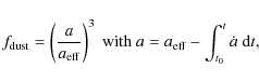 |
(A.1) |
where
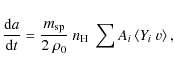 |
(A.2) |
where
For
![]() km s-1, we integrate the equation of deceleration of the dust grains with respect to the gas
km s-1, we integrate the equation of deceleration of the dust grains with respect to the gas
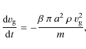
where
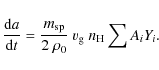 |
(A.4) |
By integrating these differential equations, the radius of the dust grains as a function of their velocity has been deduced (see Borkowski & Dwek 1995, for a complete parametrization of
Figure A.1 shows the dust mass fraction remaining in the gas after isobaric cooling from the postshock temperature
![]() to 104 K as a function of the shock velocity. The dotted line includes both thermal and inertial sputtering. For comparison, the dashed line only includes dust destruction by thermal sputtering. Our calculation for thermal sputtering with a single grain size (
to 104 K as a function of the shock velocity. The dotted line includes both thermal and inertial sputtering. For comparison, the dashed line only includes dust destruction by thermal sputtering. Our calculation for thermal sputtering with a single grain size (
![]() m) is in very good agreement with the study by Smith et al. (1996) who used a grain size distribution. For
m) is in very good agreement with the study by Smith et al. (1996) who used a grain size distribution. For
![]()
![]() 106 K, i.e.
106 K, i.e.
![]() km s-1, most of the dust is destroyed before the gas has cooled to 104 K. The gas that is heated to less than
km s-1, most of the dust is destroyed before the gas has cooled to 104 K. The gas that is heated to less than
![]() K keeps a major part of its dust content and may therefore form
K keeps a major part of its dust content and may therefore form ![]() .
.
Appendix B: Modeling the cooling of hot gas
This Appendix details how we model the cooling of the hot gas. The cooling functions used in the calculations are presented in Sect. B.1. The results are discussed in Sect. B.2.
The time dependence of both the gas temperature and the dust-to-gas mass ratio has been calculated. We start from gas at an initial postshock temperature
![]() with a galactic dust-to-gas ratio, a solar metallicity and assume equilibrium ionization. From a range of postshock temperatures up to 104 K, the isobaric gas cooling is calculated by integrating the energy balance equation which gives the rate of decrease of the gas temperature:
with a galactic dust-to-gas ratio, a solar metallicity and assume equilibrium ionization. From a range of postshock temperatures up to 104 K, the isobaric gas cooling is calculated by integrating the energy balance equation which gives the rate of decrease of the gas temperature:
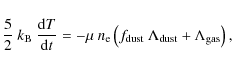
where
The time-dependent total cooling function is the sum of the dust cooling (weighted by the remaining fraction of dust mass, see Appendix A) and the gas cooling contributions.
We neglect the effect of the magnetic field on the compression of the gas. This assumption is in agreement with observations and numerical simulations, provided that the gas is not gravitationally bound (see Sect. 3.1 for details and references). The thermal gas pressure
![]() is constant in the calculations.
is constant in the calculations.
B.1 Physical processes and cooling functions
B.1.1 Cooling by atomic processes in the gas phase
The calculations of the non-equilibrium (time-dependent) ionization states and isobaric cooling rates of a hot, dust-free gas for the cooling efficiency by atomic processes has been taken from Gnat & Sternberg (2007). The electronic cooling efficiency,
![]() ,
includes the removal of electron kinetic energy via recombination with ions, collisional ionization, collisional excitation followed by line emission, and thermal bremsstrahlung.
,
includes the removal of electron kinetic energy via recombination with ions, collisional ionization, collisional excitation followed by line emission, and thermal bremsstrahlung.
![]() is shown in Fig. B.1 (black solid line
is shown in Fig. B.1 (black solid line![]() ) and reproduces the standard ``cosmic cooling curve'' presented in many papers in the literature (e.g. Sutherland & Dopita 1993). Note that most of the distinct features that appear for the ionization equilibrium case are smeared out in the nonequilibrium cooling functions and that the nonequilibrium abundances reduce the cooling efficiencies by factors of 2 to 4 (Sutherland & Dopita 1993; Gnat & Sternberg 2007). The chemical species that dominate the gas cooling are indicated in Fig. B.1 near the
) and reproduces the standard ``cosmic cooling curve'' presented in many papers in the literature (e.g. Sutherland & Dopita 1993). Note that most of the distinct features that appear for the ionization equilibrium case are smeared out in the nonequilibrium cooling functions and that the nonequilibrium abundances reduce the cooling efficiencies by factors of 2 to 4 (Sutherland & Dopita 1993; Gnat & Sternberg 2007). The chemical species that dominate the gas cooling are indicated in Fig. B.1 near the
![]() cooling curve. Over most of the temperature range, the radiative energy losses are dominated by electron-impact excitation of resonant line transitions in metal ions. At
cooling curve. Over most of the temperature range, the radiative energy losses are dominated by electron-impact excitation of resonant line transitions in metal ions. At
![]()
![]() 104 K, the cooling is mainly due to the collisional excitation of hydrogen Ly
104 K, the cooling is mainly due to the collisional excitation of hydrogen Ly![]() lines. For
lines. For
![]() K, the bremsstrahlung (free-free) radiation becomes dominant.
K, the bremsstrahlung (free-free) radiation becomes dominant.
B.1.2 Cooling by dust grains
Following the method of Dwek (1987), the cooling function of the gas by the dust via electron-grain collisions has been calculated. We adopt an MRN (Mathis et al. 1977) size distribution of dust particles, between 0.01 to ![]() m in grain radius. All the details can be found in Dwek (1987,1986), and we briefly recall here the principles of this calculation. For temperatures lower than 108 K, electron - dust grain collisions cool the gas with a cooling efficiency,
m in grain radius. All the details can be found in Dwek (1987,1986), and we briefly recall here the principles of this calculation. For temperatures lower than 108 K, electron - dust grain collisions cool the gas with a cooling efficiency,
![]()
![]() ,
given by:
,
given by:
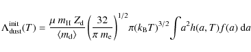 |
(B.2) |
where
The comparison in Fig. B.1 of the initial cooling efficiency by the dust,
![]() ,
and by atomic processes,
,
and by atomic processes,
![]() ,
shows that, for a dust-to-gas mass ratio of
,
shows that, for a dust-to-gas mass ratio of
![]()
![]() 10-3, the dust is initially the dominant coolant of the hot postshock gas for
10-3, the dust is initially the dominant coolant of the hot postshock gas for
![]() K. During the gas cooling, we calculate how much the grains are eroded and deduce the mass fraction of dust that remains in the cooling gas as a function of the temperature. The total cooling function (red curves in Fig. B.1) is deduced by summing the gas and dust cooling rates. We show different cooling efficiencies for different initial temperatures, corresponding to different shock velocities.
K. During the gas cooling, we calculate how much the grains are eroded and deduce the mass fraction of dust that remains in the cooling gas as a function of the temperature. The total cooling function (red curves in Fig. B.1) is deduced by summing the gas and dust cooling rates. We show different cooling efficiencies for different initial temperatures, corresponding to different shock velocities.
B.2 Results: evolution of the hot gas temperature and dust survival
The temperature profiles are shown in Fig. B.2 for different shock velocities (100 to 1000 km s-1), which corresponds to a range of preshock densities of ![]() to 2
to 2 ![]() 10-3 cm-3 for a postshock pressure of 2
10-3 cm-3 for a postshock pressure of 2 ![]() 105 K cm -3.
105 K cm -3.
Figure B.3 shows the remaining fraction of dust mass as a function of the gas temperature. In this plot, the thermal gas pressure is constant and equals the measured average thermal gas pressure of the Stephan's Quintet hot gas
![]()
![]()
![]() .
This plot illustrates a dichotomy in the evolution of the dust to gas mass ratio. On the top right side, a significant fraction of the dust survives in the gas, whereas on the left side, almost all the dust is destroyed on timescales shorter than the collision age (5
.
This plot illustrates a dichotomy in the evolution of the dust to gas mass ratio. On the top right side, a significant fraction of the dust survives in the gas, whereas on the left side, almost all the dust is destroyed on timescales shorter than the collision age (5 ![]() 106 yr). In the intercloud gas shocked at high velocities (
106 yr). In the intercloud gas shocked at high velocities (
![]() km s-1), the dust mass fraction drops rapidly. In clouds where the gas is shocked at
km s-1), the dust mass fraction drops rapidly. In clouds where the gas is shocked at
![]() km s-1, the gas retains a large fraction of its dust content (>20%).
For the gas that is heated to temperatures
T > 106 K, the dust lifetime is shorter than the gas cooling time and most of the dust is destroyed. At lower temperatures (
T < 106 K), the dust cooling rate is lower than the gas cooling rate. Then, the dust never contributes significantly to the cooling of the postshock gas. This last result is in agreement with the earlier study by Smith et al. (1996).
km s-1, the gas retains a large fraction of its dust content (>20%).
For the gas that is heated to temperatures
T > 106 K, the dust lifetime is shorter than the gas cooling time and most of the dust is destroyed. At lower temperatures (
T < 106 K), the dust cooling rate is lower than the gas cooling rate. Then, the dust never contributes significantly to the cooling of the postshock gas. This last result is in agreement with the earlier study by Smith et al. (1996).
Appendix C: Modeling H2 formation
C.1 Cooling function for T < 104 K
This section describes the cooling of clouds below 104 K and H2 formation. We use the chemistry, and the atomic and molecular cooling functions described in Flower et al. (2003) and references therein. The principal coolants are O, ![]() ,
,
![]() and OH (see Fig. 3 in Flower et al. 2003). The time evolution of the gas temperature and composition is computed at a fixed thermal gas pressure equal to that of the intercloud gas (2
and OH (see Fig. 3 in Flower et al. 2003). The time evolution of the gas temperature and composition is computed at a fixed thermal gas pressure equal to that of the intercloud gas (2 ![]() 105 K cm-3). The metallicity and the gas-to-dust mass ratio are assumed to be the solar neighbourhood values. The initial ionization state of the gas is the out-of-equilibrium value resulting from cooling from higher temperatures (Gnat & Sternberg 2007). We assume a standard value for the cosmic ray ionization rate of
105 K cm-3). The metallicity and the gas-to-dust mass ratio are assumed to be the solar neighbourhood values. The initial ionization state of the gas is the out-of-equilibrium value resulting from cooling from higher temperatures (Gnat & Sternberg 2007). We assume a standard value for the cosmic ray ionization rate of ![]()
![]() 10-17 s-1 and the UV radiation field is not considered here (see Sect. 2.2). The initial temperature is 104 K and density
10-17 s-1 and the UV radiation field is not considered here (see Sect. 2.2). The initial temperature is 104 K and density
![]() cm-3. Hydrogen is initially highly ionized. During the postshock gas cooling, hydrogen recombination occurs, the neutral gas cools,
cm-3. Hydrogen is initially highly ionized. During the postshock gas cooling, hydrogen recombination occurs, the neutral gas cools, ![]() starts to form and further cools and condenses the gas.
starts to form and further cools and condenses the gas.
![\begin{figure}
\par\includegraphics[width=8cm,clip]{11263fC2.eps}
\end{figure}](/articles/aa/full_html/2009/29/aa11263-08/img228.png) |
Figure C.2:
Isobaric cooling of the postshock gas and |
Figure C.1 presents the contribution of ![]() line emission to the total cooling function as a function of the gas temperature. It shows the cooling functions of (i) all the
line emission to the total cooling function as a function of the gas temperature. It shows the cooling functions of (i) all the ![]() lines (thick red line); (ii) the
lines (thick red line); (ii) the ![]() rotational lines S(0) to S(5) detected by Spitzer(thin red line); (iii) the total cooling efficiency in which all elements are included (green dashed line). The cooling efficiencies of some other major coolants (O in blue,
rotational lines S(0) to S(5) detected by Spitzer(thin red line); (iii) the total cooling efficiency in which all elements are included (green dashed line). The cooling efficiencies of some other major coolants (O in blue,
![]() in purple, and OH in orange) are also indicated. H2 excitation at low temperatures (
in purple, and OH in orange) are also indicated. H2 excitation at low temperatures (![]() K) is dominated by the contribution associated with
K) is dominated by the contribution associated with ![]() formation.
formation.
C.2 H2 formation
The chemical abundance profiles in the postshock gas are illustrated in Fig. C.2 as a function of time, for the same model as in Fig. C.1
From the time when the gas attains 104 K, it takes ![]()
![]() 105 yrs to form
105 yrs to form ![]() .
This time scales inversely with the dust-to-gas mass ratio. The
.
This time scales inversely with the dust-to-gas mass ratio. The ![]() formation gives rise to a shoulder in the temperature profile around 200 K. At this point, the energy released by
formation gives rise to a shoulder in the temperature profile around 200 K. At this point, the energy released by ![]() formation is roughly balanced by the cooling due to atomic oxygen (see Fig. 3 in Flower et al. 2003).
formation is roughly balanced by the cooling due to atomic oxygen (see Fig. 3 in Flower et al. 2003).
Footnotes
- ... collision
- Appendices are only available in electronic form at http://www.aanda.org
- ... spectroscopy
- Observations made at the Cerro Tololo Inter-American Observatory (CTIO).
- ... units
- G0 = 2.3
10-3 erg s-1 cm-2 at 1530 Å, Habing (1968).
- ... medium
- More detailed expressions are given in Klein et al. (1994).
- ...GALEX
- Galaxy evolution explorer.
- ... PACS
- Photodetector Array Camera and Spectrometer.
- ... yield
- The yield is the number of atoms ejected from the grain surface per incident particle.
- ... line
- The black solid line (gas cooling efficiency) is merged with the total cooling curve (red line) for
 K.
K.
All Tables
Table 1: Mass, energy and luminosity budgets of the preshock and postshock gas in the Stephan's Quintet galaxy-wide shock, directly inferred from observationsa.
Table 2: Overview of the emission of the SQ postshock gas, from observations and model predictionsa. The models are the same as those used in Fig. 5.
All Figures
| |
Figure 1:
A schematic picture of a galactic wide shock in an inhomogeneous medium. Left: a three data set image of the Stephan's Quintet system (visible red light (blue), H |
| In the text | |
![\begin{figure}
\par\includegraphics[angle=90,width=8.5cm,clip]{11263fg2.eps}
\end{figure}](/articles/aa/full_html/2009/29/aa11263-08/img110.png) |
Figure 2:
The multiphasic postshock medium. The dust lifetime, |
| In the text | |
| |
Figure 3:
Cooling and H2 formation timescales for ionized gas at 104 K as a function of the gas density and pressure (top axis). The grey horizontal bar indicates the SQ collision age, and the blue vertical bar shows the gas thermal pressure at which the |
| In the text | |
![\begin{figure}
\par\includegraphics[angle=90,width=8.5cm,clip]{11263fg4.eps}
\end{figure}](/articles/aa/full_html/2009/29/aa11263-08/img120.png) |
Figure 4:
The gas cooling and |
| In the text | |
| |
Figure 5:
|
| In the text | |
| |
Figure 6:
Schematic view of the evolutionary cycle of the gas proposed in our interpretation of optical and H2 observations of Stephan's Quintet. Arrows represent the mass flows between the H II, warm H I, warm and cold H2 gas components. They are numbered for clarity (see text). The dynamical interaction between gas phases drives the cycle. The values of the mass flows and associated timescales are derived from the
|
| In the text | |
![\begin{figure}
\par\includegraphics[angle=90,width=8cm,clip]{11263fA1.eps}
\end{figure}](/articles/aa/full_html/2009/29/aa11263-08/img197.png) |
Figure A.1:
Dust mass fraction as a function of the initial (postshock) temperature, after isobaric cooling to 104 K. The pressure is fixed to
|
| In the text | |
![\begin{figure}
\par\includegraphics[angle=90,width=15.7cm,clip]{11263fB1.eps}
\end{figure}](/articles/aa/full_html/2009/29/aa11263-08/img201.png) |
Figure B.1:
Time-dependent cooling efficiency [erg cm3 s-1] as a function of temperature during the gas cooling, for different initial conditions. The blue dashed line,
|
| In the text | |
![\begin{figure}
\par\includegraphics[angle=90,width=7.8cm,clip]{11263fB2.eps}
\end{figure}](/articles/aa/full_html/2009/29/aa11263-08/img222.png) |
Figure B.2:
Evolution of the gas temperature with time at constant pressure, from the postshock temperature to 104 K for different shock velocities (indicated on the curves in km s-1). The dashed line is for
|
| In the text | |
![\begin{figure}
\par\includegraphics[angle=90,width=7.8cm,clip]{11263fB3.eps}
\end{figure}](/articles/aa/full_html/2009/29/aa11263-08/img224.png) |
Figure B.3:
Dust mass fraction remaining as a function of the gas temperature, from the postshock temperature to 104 K for different shock velocities |
| In the text | |
![\begin{figure}
\par\includegraphics[width=7.8cm,clip]{11263fC1.eps}
\end{figure}](/articles/aa/full_html/2009/29/aa11263-08/img226.png) |
Figure C.1:
Cooling efficiency [erg s-1 cm-3 by |
| In the text | |
| |
Figure C.2:
Isobaric cooling of the postshock gas and |
| In the text | |
Copyright ESO 2009
Current usage metrics show cumulative count of Article Views (full-text article views including HTML views, PDF and ePub downloads, according to the available data) and Abstracts Views on Vision4Press platform.
Data correspond to usage on the plateform after 2015. The current usage metrics is available 48-96 hours after online publication and is updated daily on week days.
Initial download of the metrics may take a while.