| Issue |
A&A
Volume 502, Number 1, July IV 2009
|
|
|---|---|---|
| Page(s) | 91 - 111 | |
| Section | Galactic structure, stellar clusters, and populations | |
| DOI | https://doi.org/10.1051/0004-6361/200810922 | |
| Published online | 05 March 2009 | |
The nuclear star cluster of the Milky Way: proper motions and mass![[*]](/icons/foot_motif.png) ,
,
R. Schödel1 - D. Merritt2 - A. Eckart3
1 - Instituto de Astrofísica de Andalucía (IAA) - CSIC, Camino Bajo de Huétor 50, 18008 Granada, Spain
2 -
Department of Physics and Center for Computational
Relativity and Gravitation, Rochester Institute of Technology,
Rochester, NY 14623, USA
3 -
I.Physikalisches Institut, Universität zu Köln, Zülpicher Str.77, 50937 Köln, Germany
Received 5 September 2008 / Accepted 21 February 2009
Abstract
Context. Nuclear star clusters (NSCs) are located at the photometric and dynamical centers of the majority of galaxies. They are among the densest star clusters in the Universe. The NSC in the Milky Way is the only object of this class that can be resolved into individual stars. The massive black hole Sagittarius A* is located at the dynamical center of the Milky Way NSC.
Aims. In this work we examine the proper motions of stars out to distances of 1.0 pc from Sgr A*. The aim is to examine the velocity structure of the MW NSC and acquire a reliable estimate of the stellar mass in the central parsec of the MW NSC, in addition to the well-known black hole mass.
Methods. We use multi-epoch adaptive optics assisted near-infrared observations of the central parsec of the Galaxy obtained with NACO/CONICA at the ESO VLT. Stellar positions are measured via PSF fitting in the individual images and transformed into a common reference frame via suitable sets of reference stars.
Results. We measured the proper motions of more than 6000 stars within ![]() 1.0 pc of Sagittarius A*. The full data set is provided in this work. We largely exclude the known early-type stars with their peculiar dynamical properties from the dynamical analysis. The cluster is found to rotate parallel to Galactic rotation, while the velocity dispersion appears isotropic (or anisotropy may be masked by the cluster rotation). The Keplerian fall-off of the velocity dispersion due to the point mass of Sgr A* is clearly detectable only at
1.0 pc of Sagittarius A*. The full data set is provided in this work. We largely exclude the known early-type stars with their peculiar dynamical properties from the dynamical analysis. The cluster is found to rotate parallel to Galactic rotation, while the velocity dispersion appears isotropic (or anisotropy may be masked by the cluster rotation). The Keplerian fall-off of the velocity dispersion due to the point mass of Sgr A* is clearly detectable only at ![]() pc. Nonparametric isotropic and anisotropic Jeans models are applied to the data. They imply a best-fit black hole mass of
3.6+0.2-0.4
pc. Nonparametric isotropic and anisotropic Jeans models are applied to the data. They imply a best-fit black hole mass of
3.6+0.2-0.4 ![]() 106
106 ![]() .
Although this value is slightly lower than the current canonical value of 4.0
.
Although this value is slightly lower than the current canonical value of 4.0 ![]() 106
106 ![]() ,
this is the first time that a proper motion analysis provides a mass for Sagittarius A* that is consistent with the mass inferred from orbits of individual stars. The point mass of Sagittarius A* is not sufficient to explain the velocity data. In addition to the black hole, the models require the presence of an extended mass of 0.5-1.5
,
this is the first time that a proper motion analysis provides a mass for Sagittarius A* that is consistent with the mass inferred from orbits of individual stars. The point mass of Sagittarius A* is not sufficient to explain the velocity data. In addition to the black hole, the models require the presence of an extended mass of 0.5-1.5 ![]()
![]() in the central parsec. This is the first time that the extended mass of the nuclear star cluster is unambiguously detected. The influence of the extended mass on the gravitational potential becomes notable at distances
in the central parsec. This is the first time that the extended mass of the nuclear star cluster is unambiguously detected. The influence of the extended mass on the gravitational potential becomes notable at distances ![]() 0.4 pc from Sgr A*. Constraints on the distribution of this extended mass are weak. The extended mass can be explained well by the mass of the stars that make up the cluster.
0.4 pc from Sgr A*. Constraints on the distribution of this extended mass are weak. The extended mass can be explained well by the mass of the stars that make up the cluster.
Key words: instrumentation: adaptive optics - techniques: high angular resolution - stars: kinematics - Galaxy: center - Galaxy: structure
1 Introduction
After a decade of sensitive high resolution imaging with the Hubble Space Telescope the presence of nuclear star clusters (NSCs) at the centers of most galaxies has become a
well established observational fact (Matthews et al. 1999; Carollo et al. 1998; Côté et al. 2006; Phillips et al. 1996). NSCs have typical effective radii of a few pc, luminosities of
![]() ,
and masses of a few times 105 to
,
and masses of a few times 105 to
![]() (e.g. Walcher et al. 2005; Ferrarese et al. 2006). NSCs are the densest known
star clusters in the Universe. Most NSCs contain a mixed stellar population with signs of repeated episodes of star formation (Walcher et al. 2006). Recent research suggests that there exists a
fundamental relation between NSCs, supermassive black holes, and their host galaxies
(Seth et al. 2008b; Wehner & Harris 2006; Ferrarese et al. 2006; Balcells et al. 2007), similar to the relations between bulge luminosity, mass, or velocity dispersion and supermassive black hole masses
(Häring & Rix 2004; Ferrarese & Merritt 2000; Gebhardt et al. 2000; Kormendy & Richstone 1995; Tremaine et al. 2002).
The causes for these correlations are not understood, which emphasizes our need to obtain a better understanding of these objects, Unfortunately, NSCs are compact sources and therefore barely resolved in external galaxies at the diffraction limit of current 8-10 m-class and even future 30-50 m-class telescopes. Any conclusions on the structure and mass of extragalactic NSCs therefore have to be based on the properties of the integrated light of millions of stars.
(e.g. Walcher et al. 2005; Ferrarese et al. 2006). NSCs are the densest known
star clusters in the Universe. Most NSCs contain a mixed stellar population with signs of repeated episodes of star formation (Walcher et al. 2006). Recent research suggests that there exists a
fundamental relation between NSCs, supermassive black holes, and their host galaxies
(Seth et al. 2008b; Wehner & Harris 2006; Ferrarese et al. 2006; Balcells et al. 2007), similar to the relations between bulge luminosity, mass, or velocity dispersion and supermassive black hole masses
(Häring & Rix 2004; Ferrarese & Merritt 2000; Gebhardt et al. 2000; Kormendy & Richstone 1995; Tremaine et al. 2002).
The causes for these correlations are not understood, which emphasizes our need to obtain a better understanding of these objects, Unfortunately, NSCs are compact sources and therefore barely resolved in external galaxies at the diffraction limit of current 8-10 m-class and even future 30-50 m-class telescopes. Any conclusions on the structure and mass of extragalactic NSCs therefore have to be based on the properties of the integrated light of millions of stars.
Located at a distance of only 8 kpc (Reid 1993; Ghez et al. 2008; Gillessen et al. 2009; Trippe et al. 2008; Eisenhauer et al. 2005; Groenewegen et al. 2008), the center of the Milky Way (Galactic Center, GC) offers the best possibility to study an NSC in detail. The GC is obscured by about 30 mag of visual extinction and can therefore only be studied in infrared wavelengths (first pioneering observations by Becklin & Neugebauer 1968). Launhardt et al. (2002) studied the nuclear bulge of the Milky Way using COBE DIRBE data. They identified the NSC of the Milky Way (MW) and estimated its mass as
3.5 ![]() 1.5
1.5 ![]()
![]() .
The MW NSC is close to isothermal, with a power-law index around 1.8 (Eckart et al. 1993; Catchpole et al. 1990; Becklin & Neugebauer 1968; Haller et al. 1996).
Genzel et al. (2003) showed that the MW NSC contains a central stellar cusp and no flat core. Schödel et al. (2007) found that the cusp is very small (with a projected cusp radius of
0.22
.
The MW NSC is close to isothermal, with a power-law index around 1.8 (Eckart et al. 1993; Catchpole et al. 1990; Becklin & Neugebauer 1968; Haller et al. 1996).
Genzel et al. (2003) showed that the MW NSC contains a central stellar cusp and no flat core. Schödel et al. (2007) found that the cusp is very small (with a projected cusp radius of
0.22 ![]() 0.04 pc) and rather flat, with a power-law index of just 1.2
0.04 pc) and rather flat, with a power-law index of just 1.2 ![]() 0.05. It would be extremely difficult - if not impossible - to resolve this small cusp in any extragalactic system, even with 50 m-class telescopes. The cusp region is observationally dominated by
the presence of a population of young, massive stars. Their surface density follows a power-law with
0.05. It would be extremely difficult - if not impossible - to resolve this small cusp in any extragalactic system, even with 50 m-class telescopes. The cusp region is observationally dominated by
the presence of a population of young, massive stars. Their surface density follows a power-law with
![]() (Lu et al. 2008; Paumard et al. 2006), while the surface density of the
late-type stellar population is almost constant in the cusp region (Buchholz et al. 2009).
(Lu et al. 2008; Paumard et al. 2006), while the surface density of the
late-type stellar population is almost constant in the cusp region (Buchholz et al. 2009).
Like NSCs in external galaxies the Milky Way NSC consists of a mixed, old and young stellar population. Several periods of star formation have occurred in the MW NSC. The most recent star burst happened just a few million years ago (e.g., Allen et al. 1990; Paumard et al. 2006; Maness et al. 2007; Krabbe et al. 1995).
Studies of stellar dynamics have provided striking evidence for the existence of a supermassive black hole at the dynamical center of the MW NSC (see Ghez et al. 2000; Genzel et al. 2000; Eckart & Genzel 1996). The measurements of stellar orbits have provided, so far, the best evidence for its nature (e.g., Ghez et al. 2003; Schödel et al. 2003). Recent work on the orbit of the star S2/S02 gives, so far, the most accurate measurement of the mass of the black hole (![]() 4
4 ![]()
![]() )
(Ghez et al. 2008; Gillessen et al. 2009; Ghez et al. 2005; Eisenhauer et al. 2005). While some extragalactic surveys can give the impression that NSCs and supermassive black holes may be mutually exclusive (Ferrarese et al. 2006), the case of the GC and of galaxies containing both AGN and NSCs (Seth et al. 2008a) demonstrates that an NSC and a supermassive black hole can co-exist.
)
(Ghez et al. 2008; Gillessen et al. 2009; Ghez et al. 2005; Eisenhauer et al. 2005). While some extragalactic surveys can give the impression that NSCs and supermassive black holes may be mutually exclusive (Ferrarese et al. 2006), the case of the GC and of galaxies containing both AGN and NSCs (Seth et al. 2008a) demonstrates that an NSC and a supermassive black hole can co-exist.
While the mass of the supermassive black hole, Sagittarius A* (Sgr A*), at the GC has been determined with high accuracy, this is not the case for the mass and mass density of the star cluster around Sgr A*, for which there exists a large uncertainty. For example, the data presented by Haller et al. (1996) are consistent with a stellar mass between 0 and a few
![]() within 1 pc of Sgr A*. The main problem here is the lack of sufficiently large samples of stellar proper motion or line-of-sight (LOS) velocity measurements at distances sufficiently far from Sgr A* so that the velocity dispersion is not completely dominated by its mass (
within 1 pc of Sgr A*. The main problem here is the lack of sufficiently large samples of stellar proper motion or line-of-sight (LOS) velocity measurements at distances sufficiently far from Sgr A* so that the velocity dispersion is not completely dominated by its mass (![]() pc), but sufficiently close to Sgr A* in order to measure stars well within the NSC (
pc), but sufficiently close to Sgr A* in order to measure stars well within the NSC (
![]() pc) and thus to avoid significant contamination by stars in the nuclear disk, bulge, or foreground.
pc) and thus to avoid significant contamination by stars in the nuclear disk, bulge, or foreground.
Due to the lack of data, estimates of the enclosed mass profile at the GC were up to now heavily influenced by modeling assumptions, such as adopting some ad hoc value for the velocity dispersion at large distances, or by estimates of the enclosed stellar and BH mass based on measurements of gas velocities (e.g., Schödel et al. 2002; Genzel et al. 1996). Schödel et al. (2007) have re-analyzed this issue and concluded that the mass of the star cluster in the central parsec is possibly significantly higher than previously assumed. Their claim is based on observational data that indicate that the measured line-of-sight velocity dispersion of late type stars within ![]() 0.8 pc of Sgr A* remains apparently constant, with a value around 100 km s-1(Zhu et al. 2008; Figer et al. 2003). This contrasts with the expectation that the velocity dispersion would show a Keplerian decrease over the entire central parsec if only the BH point mass were
important. Additionally, Reid et al. (2007) found that the mass of Sgr A* is not sufficient to keep the maser star IRS 9 on a bound orbit and that this may imply the existence of several
0.8 pc of Sgr A* remains apparently constant, with a value around 100 km s-1(Zhu et al. 2008; Figer et al. 2003). This contrasts with the expectation that the velocity dispersion would show a Keplerian decrease over the entire central parsec if only the BH point mass were
important. Additionally, Reid et al. (2007) found that the mass of Sgr A* is not sufficient to keep the maser star IRS 9 on a bound orbit and that this may imply the existence of several
![]() of extended mass within
of extended mass within
![]() pc of the black hole. This appears to contradict earlier mass estimates, like the ones mentioned above, that indicate a negligible amount of extended mass within 1 pc of Sgr A*. Using the measured radial velocity dispersions of late type stars in the central parsec in combination with the density profile of the NSC Schödel et al. (2007) provide a simple model (using the Bahcall-Tremaine mass estimator and assuming no rotation, isotropy, and that the velocity dispersion stays constant beyond the central parsec, where it was measured) of enclosed mass vs. distance from Sgr * that is consistent with up to a few
pc of the black hole. This appears to contradict earlier mass estimates, like the ones mentioned above, that indicate a negligible amount of extended mass within 1 pc of Sgr A*. Using the measured radial velocity dispersions of late type stars in the central parsec in combination with the density profile of the NSC Schödel et al. (2007) provide a simple model (using the Bahcall-Tremaine mass estimator and assuming no rotation, isotropy, and that the velocity dispersion stays constant beyond the central parsec, where it was measured) of enclosed mass vs. distance from Sgr * that is consistent with up to a few
![]() of extended mass within 1 pc of Sgr A*. The key difference to mass
profiles presented in earlier works is the realization that the projected velocity dispersion follows a clear Kepler-law only out to projected distances
of extended mass within 1 pc of Sgr A*. The key difference to mass
profiles presented in earlier works is the realization that the projected velocity dispersion follows a clear Kepler-law only out to projected distances ![]() pc from Sgr A*, but remains apparently constant at
pc from Sgr A*, but remains apparently constant at ![]() pc.
pc.
The mass and mass density of the nuclear star cluster around Sgr A* is of great importance for understanding the dynamics of this complex system. It can have strong implications for topics such as star formation, the rate of stellar collisions, the relaxation time, cusp and black hole growth, and the rate of gravitational wave emission events (for an overview of stellar processes near massive black holes, see, e.g. Alexander 2007). In order to provide reliable
estimates of the mass of the MW NSC we therefore present in this work a comprehensive sample of stellar proper motions within ![]() 1 pc of Sgr A*. The new data allow us to present accurate estimates of the enclosed mass vs. distance at the center of the Milky Way.
1 pc of Sgr A*. The new data allow us to present accurate estimates of the enclosed mass vs. distance at the center of the Milky Way.
Sections 2-5 are largely technical and describe the data processing and how the proper motions of stars in the GC were derived. Readers who are primarily interested in the main results of our analysis, can go directly to Sect. 6.
2 Observations and data reduction
The imaging data used in this work were obtained with the near-infrared (NIR) camera and adaptive optics (AO) system CONICA/NAOS (short: NaCo; Lenzen et al. 2003; Rousset et al. 2003) at the ESO VLT
unit telescope 4![]() . For images centered on Sgr A* the
. For images centered on Sgr A* the
![]() supergiant IRS 7 was used to close the loop of the AO, using the unique NIR wavefront sensor NAOS is equipped with. A guide star with
supergiant IRS 7 was used to close the loop of the AO, using the unique NIR wavefront sensor NAOS is equipped with. A guide star with
![]() located
located ![]() 19'' NE of
Sgr A* was used as reference for the AO for the images offset from Sgr A*. The sky background was measured on a largely empty patch of sky, a dark cloud about 400'' north and 713'' east of the GC. Data reduction was standard, with sky subtraction, bad pixel correction, and flat fielding. The field-of-view (FOV) of a single exposure is 28''
19'' NE of
Sgr A* was used as reference for the AO for the images offset from Sgr A*. The sky background was measured on a largely empty patch of sky, a dark cloud about 400'' north and 713'' east of the GC. Data reduction was standard, with sky subtraction, bad pixel correction, and flat fielding. The field-of-view (FOV) of a single exposure is 28'' ![]() 28''. The observations were dithered (either applying a fixed rectangular pattern or a random pattern) in order to cover a FOV
of about 40''
28''. The observations were dithered (either applying a fixed rectangular pattern or a random pattern) in order to cover a FOV
of about 40'' ![]() 40''.
40''.
The majority of the images were taken by dithering around a position roughly centered on Sgr A*. These data will be referred to in this article as the center data set. There are three observations that were centered on a field roughly 20'' NE of Sgr A*, the offset data set. Those images were used for determining the velocity dispersion in the MW NSC at projected distances from Sgr A* out to 1.15 pc. The pixel scale of all NaCo data used in this work is 0.027'' per pixel. Details of the observations are listed in Table 1. Mosaic images of the two observed fields are shown in Figs. 1 and 2.
Table 1: Details of the imaging observations used in this work.
![\begin{figure}
\par\includegraphics[width=9cm,clip]{0922fig1.eps}
\end{figure}](/articles/aa/full_html/2009/28/aa10922-08/img47.png) |
Figure 1: Mosaic image of the observations from 1 June 2006. A logarithmic gray scale has been adopted. The positions of IRS 7 and Sgr A* are indicated. North is up and east is to the left. Offsets in arcseconds from Sgr A* are indicated. Note that this mosaic image is only roughly astrometric. A constant pixel scale of 0.027'' per pixel has been assumed. Any residual net rotation of the image derotator has not been determined, i.e. the image may have a non-zero rotation angle (<1 deg). This may lead to offsets of up to a few tenths of arcseconds near the edge of the field. |
| Open with DEXTER | |
3 Photometry and astrometry
For accurate error assessment and in order to avoid any additional errors introduced by the mosaicing process, we did not combine the individual frames into mosaic images. Photometry and astrometry were instead done on individual exposures. This allowed us to compare multiple independent measurements for each star at each epoch. The number of individual frames per epoch is listed in Col. 4 of Table 1. The PSF fitting program package StarFinder (Diolaiti et al. 2000) was used. Since the 28'' ![]() 28'' (1024
28'' (1024 ![]() 1024 pixel) field-of-view (FOV) of the NaCo S27 camera, that was used for all observations, is larger than
the isoplanatic angle of near-infrared adaptive optics observations (
1024 pixel) field-of-view (FOV) of the NaCo S27 camera, that was used for all observations, is larger than
the isoplanatic angle of near-infrared adaptive optics observations (![]() 10-15''), the images were divided into sub-frames of
10-15''), the images were divided into sub-frames of ![]() 7''
7'' ![]() 7'' size, i.e. with angular diameters smaller than the isoplanatic angle. PSF extraction, followed by astrometry and photometry was done on each of the individual sub-frames. In order to minimize any uncertainties related to PSF extraction, each image was divided by a rectangular pattern in many overlapping sub-frames. The
step size between the mid-points of the sub-frames was chosen as half the width of the sub-frames.
7'' size, i.e. with angular diameters smaller than the isoplanatic angle. PSF extraction, followed by astrometry and photometry was done on each of the individual sub-frames. In order to minimize any uncertainties related to PSF extraction, each image was divided by a rectangular pattern in many overlapping sub-frames. The
step size between the mid-points of the sub-frames was chosen as half the width of the sub-frames.
PSF extraction was done by identifying all suitable PSF reference stars within each sub-frame (all potential PSF reference stars for the entire FOV were marked previously by hand on a large mosaic
image). The noise for each sub-frame was determined from the read-out and photon noise (algorithm provided by StarFinder). In order to improve the PSF, the StarFinder algorithm was run once on the sub-frame with a detection threshold of ![]() .
PSF extraction was then repeated. Since the quality of the PSF deteriorates in the wings, the PSF had to be truncated. We used a circular mask with radius 20 pixel (about 6 times the FWHM of the PSF). The StarFinder algorithm was then applied to the sub-frame, using two iterations with a
.
PSF extraction was then repeated. Since the quality of the PSF deteriorates in the wings, the PSF had to be truncated. We used a circular mask with radius 20 pixel (about 6 times the FWHM of the PSF). The StarFinder algorithm was then applied to the sub-frame, using two iterations with a ![]() threshold and a correlation threshold of 0.7.
threshold and a correlation threshold of 0.7.
Measurements of stars in overlapping sub-frames were averaged. With the exception of the stars near the edge of the field, there were 4 measurements of each source. The uncertainties derived from these measurements were smaller than the formal uncertainties of the PSF fitting routine.
![\begin{figure}
\par\includegraphics[width=9cm,clip]{0922fig2.eps}
\end{figure}](/articles/aa/full_html/2009/28/aa10922-08/img51.png) |
Figure 2: Mosaic image of the observations from 28 May 2008. The center of the image is offset about 20'' NE from Sgr A*. A logarithmic gray scale has been adopted. The positions of IRS 7, Sgr A*, and of the young and massive star IRS 8, that is surrounded by a bow-shock (Geballe et al. 2006), are indicated. North is up and east is to the left. Offsets in arcseconds from Sgr A* are indicated. Please note that this mosaic image is only roughly astrometric (see comments in caption of Fig. 1). |
| Open with DEXTER | |
The cores of saturated sources were repaired during the PSF extraction process. The detected stars have magnitudes
![]() .
Any spurious sources that may still be present in the data at this point were eliminated later when merging the source lists of the various exposures for each epoch after alignment with the reference frame. Each star had to be detected in multiple
exposures (see Appendix A).
.
Any spurious sources that may still be present in the data at this point were eliminated later when merging the source lists of the various exposures for each epoch after alignment with the reference frame. Each star had to be detected in multiple
exposures (see Appendix A).
4 Transformation into a common reference frame
Since there is no absolute frame of reference available for determining the proper motions of stars at the GC, one has to transform the stellar positions into a common reference frame using a large number of stars with either known proper motions or with the assumption that their motions cancel on average. The problem has been described previously in various publications, e.g., Eckart & Genzel (1997) or Ghez et al. (1998).
In this work, we present proper motions on a much larger FOV than what has been published on the GC before (but see also Trippe et al. 2008, which appeared shortly before this work). The large FOV means that significant dither offsets from the initial pointing (of the order 6''-8'') had to be applied. Since this implies that stars come to lie on different areas of the detector, camera distortions may become of considerable importance in this case. Therefore, special care has to be taken when aligning all stellar positions to a common reference frame. This procedure is key to obtaining accurate proper motion measurements. For the sake of repeatability of the experiment we consider it important to describe our applied methodology in detail. However, since this is a largely technical issue that may not be of interest to many readers, we describe this procedure in Appendix A.
5 Proper motions
5.1 Center field
After alignment of the stars into a common reference frame, stars were matched by searching within a circle of 2 pixels radius around the position in the reference frame. This radius is smaller than the FWHM of the AO data, which avoids mismatching. It is large enough in order to detect stars with proper motion velocities up to 500 km s-1 in each coordinate. Sources with proper motions exceeding this value would be missed by this analysis, but should be extremely rare (see histogram in Fig. 10). Sources with such high velocities can easily be detected by visual inspection of images taken about 2 years apart. We did not find such fast moving sources in a visual inspection (limited to
![]() )
of the images. Matching of the stars within 1'' of Sgr A*, where source density is highest and proper motion velocities exceed several hundred km s-1 was done manually. Proper motions were subsequently determined by linear fits to the measured positions vs. time. In order to be included in our proper motion sample, a star had to be detected in at least 4 different years. This assures an adequate
sampling of its proper motion. The reasons why certain stars are not present in all the epochs are, among others, variable quality of the data (Strehl ratio, exposure time, noise introduced by read-out electronics, etc.), a variable FOV of the observations, or, in some exceptional cases, strong orbital acceleration of stars close to Sgr A* (R<0.5''). More than 80% of all stars in the common overlap area that are not present at all epochs (corresponding to
)
of the images. Matching of the stars within 1'' of Sgr A*, where source density is highest and proper motion velocities exceed several hundred km s-1 was done manually. Proper motions were subsequently determined by linear fits to the measured positions vs. time. In order to be included in our proper motion sample, a star had to be detected in at least 4 different years. This assures an adequate
sampling of its proper motion. The reasons why certain stars are not present in all the epochs are, among others, variable quality of the data (Strehl ratio, exposure time, noise introduced by read-out electronics, etc.), a variable FOV of the observations, or, in some exceptional cases, strong orbital acceleration of stars close to Sgr A* (R<0.5''). More than 80% of all stars in the common overlap area that are not present at all epochs (corresponding to ![]() 10% of all stars) are faint stars (
10% of all stars) are faint stars (
![]() ), whose detection and measurement is particularly affected by the data quality.
), whose detection and measurement is particularly affected by the data quality.
Outliers in the data were removed by first applying an unweighted fit (in order to avoid to be biased by spurious erroneous measurements) and rejecting any data point with a deviation >![]() from the fitted position. Then the linear fit was repeated by weighting the
positions according to their
from the fitted position. Then the linear fit was repeated by weighting the
positions according to their ![]() uncertainties. Although we have not investigated the exact causes of these outliers - there may be various causes - we believe that the main reason for the
spurious data points is confusion with unresolved (maybe in a few cases also resolved) sources in the dense NSC. This source of systematic uncertainty has been investigated in detail by Ghez et al. (2008). This hypothesis is supported by the fact that outliers are largely associated with faint stars. More than 75% (97%) of the outliers are associated with stars fainter than
uncertainties. Although we have not investigated the exact causes of these outliers - there may be various causes - we believe that the main reason for the
spurious data points is confusion with unresolved (maybe in a few cases also resolved) sources in the dense NSC. This source of systematic uncertainty has been investigated in detail by Ghez et al. (2008). This hypothesis is supported by the fact that outliers are largely associated with faint stars. More than 75% (97%) of the outliers are associated with stars fainter than
![]() .
As concerns the numbers of removed data points, 22% of the stars had one data point removed, 10% two, and 8% three or more. The above mentioned criterion that position measurements had to be available for at least 4 different years was applied only after removing the outliers.
.
As concerns the numbers of removed data points, 22% of the stars had one data point removed, 10% two, and 8% three or more. The above mentioned criterion that position measurements had to be available for at least 4 different years was applied only after removing the outliers.
A distance of 8.0 kpc to the GC was assumed. A pixel scale of 0.027''/pixel was adopted for the camera detector (see ESO manual con NAOS/CONICA, available at the ESO web site). The adopted pixel scale is somewhat smaller than the value given in the manual (0.02715''/pixel). However, this difference will lead to a systematic error of less than ![]() on the measured proper motions.
on the measured proper motions.
In the top panel of Fig. 3 we show a plot of reduced ![]() vs. Ks-band magnitude for the proper motion fits. As can be seen,
vs. Ks-band magnitude for the proper motion fits. As can be seen,
![]() is close to 1.0 for stars brighter than mag
is close to 1.0 for stars brighter than mag
![]() ,
but increases toward fainter magnitudes. This
indicates that there are measurement uncertainties that we have not taken into account and that become increasingly important for faint stars. Since the positional uncertainty for each star is derived from multiple images at each epoch, the positional uncertainty for a given epoch can be expected to be correctly determined. This implies that the missing source of uncertainty must be due to systematic deviations between the epochs. This means that while a stellar position may be
measured with high precision in one epoch, its accuracy may in fact be subject to additional errors. We believe that the most probable source of error that has not been taken into account in our analysis consists of systematic deviations of the positions of faint stars due to their motion through an extremely dense stellar field and bright background due to unresolved stars. This source of error is described and analyzed in detail for the star S2/S0-2 in a recent paper by Ghez et al. (2008).
,
but increases toward fainter magnitudes. This
indicates that there are measurement uncertainties that we have not taken into account and that become increasingly important for faint stars. Since the positional uncertainty for each star is derived from multiple images at each epoch, the positional uncertainty for a given epoch can be expected to be correctly determined. This implies that the missing source of uncertainty must be due to systematic deviations between the epochs. This means that while a stellar position may be
measured with high precision in one epoch, its accuracy may in fact be subject to additional errors. We believe that the most probable source of error that has not been taken into account in our analysis consists of systematic deviations of the positions of faint stars due to their motion through an extremely dense stellar field and bright background due to unresolved stars. This source of error is described and analyzed in detail for the star S2/S0-2 in a recent paper by Ghez et al. (2008).
The systematic increase of
![]() vs. brightness can be fitted well with a simple line in log-log space. This fit is used to re-normalize the
vs. brightness can be fitted well with a simple line in log-log space. This fit is used to re-normalize the
![]() -values of the stars before determining the overall distribution of
-values of the stars before determining the overall distribution of
![]() -values. The latter is shown in the middle panel of Fig. 3 and can be seen to peak close to 1.0 as expected. Please note that we do not deal with an ideal
-values. The latter is shown in the middle panel of Fig. 3 and can be seen to peak close to 1.0 as expected. Please note that we do not deal with an ideal
![]() -distribution because the number of degrees of freedom varies, depending on the number of measurements available per star.
-distribution because the number of degrees of freedom varies, depending on the number of measurements available per star.
![\begin{figure}
\par\includegraphics[width=9cm,clip]{0922fig3.eps}
\end{figure}](/articles/aa/full_html/2009/28/aa10922-08/img60.png) |
Figure 3:
Error analysis for center field data. Top: plot of log(
|
| Open with DEXTER | |
In order to avoid under- (in the majority of cases, see top panel of Fig. 3) or over-estimating the uncertainties of the inferred velocities, the uncertainties were re-scaled with the corresponding
![]() of the fit. This procedure is viable because we can assume that a linear fit is in fact a reasonable model for our data. The distribution of the velocity uncertainties after re-scaling is shown in the bottom panel of Fig. 3. The
percentage of sources with
of the fit. This procedure is viable because we can assume that a linear fit is in fact a reasonable model for our data. The distribution of the velocity uncertainties after re-scaling is shown in the bottom panel of Fig. 3. The
percentage of sources with
![]() km s-1 is
km s-1 is ![]()
![]() .
More than
.
More than ![]() of the stars have velocity uncertainties
of the stars have velocity uncertainties
![]() km s-1.
km s-1.
After application of the methodology described above, we obtained a list of 6124 stars with measured proper motions for the central field. The positions and velocities of the measured stars are illustrated in Fig. 4. Some important features can be seen at first glance: the velocities are highest near Sgr A* (at the origin of the coordinate system) and decrease with distance from the black hole; some apparently coherently moving groups of stars can be seen at a few arcseconds distance from Sgr A*, related to known groups (IRS 13, IRS 16) and/or the disk(s) of young stars in the central half parsec (see Genzel et al. 2003; Lu et al. 2005; Schödel et al. 2005; Paumard et al. 2006; Levin & Beloborodov 2003); at larger distances the directions of the proper motions appear to be random.
The influence of the proper motions of the reference stars on the accuracy of the coordinate transformation was checked by iterating the described procedure to obtain proper motions. The initially measured proper motions of the reference stars were used to calculate their correct positions for each epoch. The resulting change in the measured stellar velocities for all sources is insignificant (![]()
![]() ). Hence, the approach of using a dense grid of evenly
sampled reference stars delivers very stable solutions for the coordinate transformation. As a further test, we repeated the above procedure by applying just a second order transformation
(
). Hence, the approach of using a dense grid of evenly
sampled reference stars delivers very stable solutions for the coordinate transformation. As a further test, we repeated the above procedure by applying just a second order transformation
(
![]() in Eqs. (A.1) and (A.2)) of the stellar positions into the reference frame. Again, the deviations were insignificant.
in Eqs. (A.1) and (A.2)) of the stellar positions into the reference frame. Again, the deviations were insignificant.
In a final step, the pixel positions of the stars were transformed into the radio reference frame as established by maser stars. The positions and proper motions of the SiO masers IRS 15NE, IRS 7, IRS 17, IRS 10EE, IRS 28, IRS 9, and IRS 12N are taken from the values measured by Reid et al. (2007), while their IR positions and proper motions are taken from the linear fits derived from our data set. A first order transformation was applied (
![]() in Eqs. (A.1) and (A.2)). In order to estimate the uncertainty of the transformation into the radio frames, the transformation parameters were estimated repeatedly with subsets of 6 out of the 7 maser stars. A smoothed (by applying a Gaussian filter of 2.0'' FWHM) map of the systematic uncertainty of the astrometric position in the radio frame was created and is shown in Fig. 5. Near Sgr A* an absolute positional rms accuracy of
in Eqs. (A.1) and (A.2)). In order to estimate the uncertainty of the transformation into the radio frames, the transformation parameters were estimated repeatedly with subsets of 6 out of the 7 maser stars. A smoothed (by applying a Gaussian filter of 2.0'' FWHM) map of the systematic uncertainty of the astrometric position in the radio frame was created and is shown in Fig. 5. Near Sgr A* an absolute positional rms accuracy of ![]() 15 milli-arcsec is reached. Probably the most important effects that limit the accuracy of the alignment with the astrometric reference frame are the uncertainty of the proper motions
of the maser stars in the IR frame and residual distortions in the IR reference frame because we did not determine a distortion solution for our 2006 reference frame (see Sect. A). The maser stars are saturated in the data of most epochs, with the positional information therefore being based mainly on the PSF wings of these stars. The proper motions of the maser stars in the infrared and radio frames agree very well (see Sect. 5.3 below).
15 milli-arcsec is reached. Probably the most important effects that limit the accuracy of the alignment with the astrometric reference frame are the uncertainty of the proper motions
of the maser stars in the IR frame and residual distortions in the IR reference frame because we did not determine a distortion solution for our 2006 reference frame (see Sect. A). The maser stars are saturated in the data of most epochs, with the positional information therefore being based mainly on the PSF wings of these stars. The proper motions of the maser stars in the infrared and radio frames agree very well (see Sect. 5.3 below).
![\begin{figure}
\par\includegraphics[width=17cm,clip]{0922fig4.eps}
\end{figure}](/articles/aa/full_html/2009/28/aa10922-08/img68.png) |
Figure 4: Map of stars with measured proper motions in the GC central field. North is up and east is to the left. Arrows indicate magnitude and direction of the proper motion velocities. The black arrow in the lower left corner indicates the length of a 1000 km s-1 arrow. Positions and velocities of the stars are listed in in Table B.1. Early-type stars, identified by Paumard et al. (2006) and Buchholz et al. (2009) are indicated by red arrows. The small red circle marks the best candidate for a star escaping the cluster. |
| Open with DEXTER | |
The intrinsic H-K colour of the stars in the GC field is almost (to within ![]() 0.1 mag) independent of their stellar type (see discussion in Schödel et al. 2007). Therefore H-K-colours can be used to get a fairly accurate value of the extinction toward individual stars. We identified about 30 foreground stars in the proper motion sample by their low extinction (AK<2.0) and removed them from the sample. Here, we used the H-K values and extinction
measurements of Schödel et al. (in preparation).
0.1 mag) independent of their stellar type (see discussion in Schödel et al. 2007). Therefore H-K-colours can be used to get a fairly accurate value of the extinction toward individual stars. We identified about 30 foreground stars in the proper motion sample by their low extinction (AK<2.0) and removed them from the sample. Here, we used the H-K values and extinction
measurements of Schödel et al. (in preparation).
The final list of stars with their fitted positions in 2004.44, their measured proper motions, and magnitudes is presented in Table B.1. Since the few million year-old population of early-type stars in the central parsec has particular kinematic properties (see Lu et al. 2008; Paumard et al. 2006), we identified early-type stars in the sample. We find 79 early-type stars from the spectroscopic analysis by Paumard et al. (2006) (their Table 2) and 202 additional early-type candidates from the photometric analysis of Buchholz et al. (2009). Spectroscopically identified early-type stars are marked with a ``1'' and photometrically identified ones with a ``2'' in the last column of Table B.1. We recommend future users of this list to cross-check the identifications with the latest available
publications. Note also that identification of spectral type was only available for a fraction of the stars, leaving a large number of stars unidentified (near the edge of the FOV and all stars
fainter than
![]() ). Note also that the number of early-type stars is much smaller than the overall number of stars. Also, their surface density decreases rapidly beyond a few arcseconds distance from Sgr A* (Lu et al. 2008; Paumard et al. 2006). Therefore, their weight on the measured statistical properties of the entire cluster is almost negligible, except in the innermost arcseconds. Nevertheless, we will largely exclude the identified early-type stars from our analysis due to their special dynamical properties.
). Note also that the number of early-type stars is much smaller than the overall number of stars. Also, their surface density decreases rapidly beyond a few arcseconds distance from Sgr A* (Lu et al. 2008; Paumard et al. 2006). Therefore, their weight on the measured statistical properties of the entire cluster is almost negligible, except in the innermost arcseconds. Nevertheless, we will largely exclude the identified early-type stars from our analysis due to their special dynamical properties.
Table 2: Measured proper motions, in the infrared frame, of the maser stars used for astrometric alignment.
The reader should keep in mind that orbital accelerations have not been taken into account in the present analysis. This is the reason why the position of the star S2 in Table B.1 (second line) has an offset from its actual position in 2004.44 that is ![]() 20 mas larger than the astrometric uncertainty at its position. This kind of additional uncertainty only affects very few (<5) stars. We did not exclude them from our sample because they provide important information on the velocity dispersion near Sgr A*.
20 mas larger than the astrometric uncertainty at its position. This kind of additional uncertainty only affects very few (<5) stars. We did not exclude them from our sample because they provide important information on the velocity dispersion near Sgr A*.
![\begin{figure}
\par\includegraphics[width=8.8cm,clip]{0922fig5.eps}
\end{figure}](/articles/aa/full_html/2009/28/aa10922-08/img115.png) |
Figure 5: Map of the systematic positional uncertainty of the astrometric positions of the stars listed in Table B.1. Contours are plotted in steps of 10 mas from 20 to 80 mas. |
| Open with DEXTER | |
5.2 Offset field
The results of the proper motion analysis for the offset field serve as cross-validation of our results, but were not used for the subsequent modeling because the quality of the proper motions is lower (only three epochs compared to 11 for the center field) and the radial range of the proper motions is not extended significantly. The data and results are described in Appendix B.
5.3 Relative motion between radio and infrared frame of reference
A question of great interest is whether there exists any relative motion between the radio and near-infrared reference frames. The black hole, Sgr A* is at rest in the so-called radio reference frame. The positions and velocities of the maser stars have been measured in the radio frame via VLBI observations (see, e.g., Reid et al. 2007). When deriving the positions and proper motions of stars in the infrared frame, we assume that the cluster of stars has an average velocity of zero (see also Appendix A). Hence, comparing the velocities of the maser stars measured in the radio and in the infrared frames is an important cross-check. Their velocities are expected to be identical in the two reference frames. Any significant non-zero average value of the difference between the masers' radio and infrared proper motions would imply a relative movement between Sgr A* and the star cluster.
We list the measured proper motions in the infrared frame of the 7 maser stars used for the astrometric alignment in Table 2. All infrared proper motions of the maser
stars agree within <![]() with their proper motions as measured by VLBI (Reid et al. 2007).
with their proper motions as measured by VLBI (Reid et al. 2007).
The weighted mean difference between the velocities of the seven maser stars in the radio and the IR frames is in right ascension 0.01 ![]() 0.10 mas yr-1 (unweighted: 0.04
0.10 mas yr-1 (unweighted: 0.04 ![]() 0.45 mas yr-1) toward the east and in declination 0.22
0.45 mas yr-1) toward the east and in declination 0.22 ![]() 0.11 mas yr-1 (unweighted: 0.07
0.11 mas yr-1 (unweighted: 0.07 ![]() 0.67 mas yr-1) toward the south. At a distance of 8.0 kpc a proper motion of 1 mas yr-1 corresponds to
0.67 mas yr-1) toward the south. At a distance of 8.0 kpc a proper motion of 1 mas yr-1 corresponds to ![]() 38 km s-1. Converting the weighted mean motions to km s-1 this means that the radio reference frame moves relative to the IR frame with 0.4
38 km s-1. Converting the weighted mean motions to km s-1 this means that the radio reference frame moves relative to the IR frame with 0.4 ![]() 3.8 km s-1 toward east and 8.4
3.8 km s-1 toward east and 8.4 ![]() 3.8 km s-1 toward south. Following Reid et al. (2007) an additional systematic error of 5 km s-1 should be added to these values in quadrature in order to take into account the removal of the average motion of the IR frame (IR-motions are derived by assuming that the net motion of the reference stars is 0). This results in a
3.8 km s-1 toward south. Following Reid et al. (2007) an additional systematic error of 5 km s-1 should be added to these values in quadrature in order to take into account the removal of the average motion of the IR frame (IR-motions are derived by assuming that the net motion of the reference stars is 0). This results in a ![]() uncertainty of 6.4 km s-1 on the relative motion between the radio and IR reference frames. This reduces the significance of the southward motion to less than
uncertainty of 6.4 km s-1 on the relative motion between the radio and IR reference frames. This reduces the significance of the southward motion to less than ![]() .
Considering additionally that the weighted relative mean velocity between the radio and IR frames in Reid et al. (2007) is a net northward motion, while we measure a southward motion here, we can safely conclude that the result is consistent with
no detectable motion. We conclude that within the accuracy of the presented measurements there is no detectable relative motion between the infrared and the radio reference frames and consequently between the stellar cluster and the central supermassive black hole Sgr A*. This is consistent with our expectations. The expected rms velocity of the BH due to gravitational perturbations from stars is
.
Considering additionally that the weighted relative mean velocity between the radio and IR frames in Reid et al. (2007) is a net northward motion, while we measure a southward motion here, we can safely conclude that the result is consistent with
no detectable motion. We conclude that within the accuracy of the presented measurements there is no detectable relative motion between the infrared and the radio reference frames and consequently between the stellar cluster and the central supermassive black hole Sgr A*. This is consistent with our expectations. The expected rms velocity of the BH due to gravitational perturbations from stars is ![]() 0.2 km s-1 (Merritt et al. 2007).
0.2 km s-1 (Merritt et al. 2007).
6 Velocity structure of the NSC
![\begin{figure}
\par\includegraphics[width=17cm,clip]{0922fig6.eps}
\end{figure}](/articles/aa/full_html/2009/28/aa10922-08/img117.png) |
Figure 6: Top: mean projected radial and tangential velocities vs. projected distance from Sgr A* ( left) and vs. angle east of north ( right). Mean values and the standard deviations annotated in the plots were calculated from the unweighted data points. Bottom: projected radial (green) and tangential (blue) velocity dispersions in the GC nuclear star cluster vs. projected distance from Sgr A* ( left) and vs. angle east of north ( right). These plots are based on the center data set (see Fig. 1) under the exclusion of identified early-type stars. |
| Open with DEXTER | |
6.1 First look
The velocity data were converted from directions along right ascension and declination into physically more meaningful projected radial and tangential velocities with respect to Sgr A*. The mean projected radial and tangential velocities and velocity dispersions for the center data set, excluding identified early-type stars, are shown in Fig. 6. The top left panel shows the mean velocities vs. distance from Sgr A* in radial bins. The mean velocities are generally close to zero. There are some deviations from zero, but also larger error bars, at ![]() .
In these innermost bins stellar numbers are lower because of the correspondingly smaller surface
areas. Also, the relative number of early-type stars increases toward Sgr *. This tends to decrease additionally the number of stars in the bins (early-type stars were excluded from this analysis). There are no significant indications of net expansion, contraction, or rotation of
parts of the cluster in the plane of the sky. An overall net rotation of the entire cluster in the plane of the sky with a constant angular velocity cannot be detected by our method. The reason is that the coordinate transformation between the epochs is based on the assumption that the overall motion of the stars is zero. Rotation of parts of the cluster, such as the disk of early-type stars, can be detected, however (see Fig. 4).
.
In these innermost bins stellar numbers are lower because of the correspondingly smaller surface
areas. Also, the relative number of early-type stars increases toward Sgr *. This tends to decrease additionally the number of stars in the bins (early-type stars were excluded from this analysis). There are no significant indications of net expansion, contraction, or rotation of
parts of the cluster in the plane of the sky. An overall net rotation of the entire cluster in the plane of the sky with a constant angular velocity cannot be detected by our method. The reason is that the coordinate transformation between the epochs is based on the assumption that the overall motion of the stars is zero. Rotation of parts of the cluster, such as the disk of early-type stars, can be detected, however (see Fig. 4).
A comparison between proper motions of maser stars in the radio and infrared reference frames allows some check on the rotation of the cluster in the plane of the sky. It does not provide any evidence for rotation in the plane of the sky (see Sect. 6.2). The top right panel of Fig. 6 shows the mean velocities of the stars vs. angle on the sky, measured east of north. They are close to zero, but a possibly significant sinusoidal pattern can be discerned, especially in the tangential mean velocities. This is probably the imprint of an overall rotation of the cluster (see below) in the Galactic plane.
The bottom left panel of Fig. 6 shows a plot of the projected radial and tangential velocity dispersion vs. distance from Sgr A*. With the exception of the region at R<6'' the data suggest isotropy with considerable accuracy. Any deviations from isotropy at R<6'' may be due to either worse statistics (smaller surface area and exclusion of early-type stars) and/or the presence of not identified early-type stars in the sample, which may follow a coherent rotation pattern (see Lu et al. 2006; Genzel et al. 2003; Paumard et al. 2006, and Fig. 4). The plot of the velocity dispersion vs. angle on the sky (bottom right) shows a sinusoidal pattern for the projected tangential velocity dispersion, which is probably due to rotation of the cluster in the Galactic plane (see Sect. 6.3 below).
6.2 Rotation in the plane of the sky
The proper motions were derived by a third order polynomial alignment of the stellar positions with the reference epoch. This procedure excludes detecting rotation of the entire cluster with a constant angular velocity in the plane of the sky. It does, however, not exclude detecting rotation of sub-groups of star, such as the early type stars within a few arcseconds from Sgr A* (see Fig. 4) that is described in detail, e.g., in Paumard et al. (2006) and Lu et al. (2008).
The maser stars offer, in principle, the possibility of a cross check because their velocity have been measured independently in the radio reference frame. In Fig. 7 we show a plot of the projected tangential proper motions of the maser stars as measured in the radio and infrared frames, as well as the respective differences. While 7 stars are far too less for any statistically meaningful test of the absolute rotation of the cluster in the plane of the sky, it is at least possible to check for any relative rotation between the radio and infrared frames.
The mean difference (radio minus infrared) tangential proper motion is -0.5 km s-1 with a standard deviation of 21.8 km s-1. A linear fit to the difference values results in
a slope of 3.8 ![]() 11.1 km s-1 arcsec-1 (uncertainty re-scaled to a reduced
11.1 km s-1 arcsec-1 (uncertainty re-scaled to a reduced ![]() of 1). We conclude that there is no detectable relative rotation between the radio and infrared reference frames. Future measurements with longer time baselines and more maser
stars can help to reduce the still large uncertainty of this comparison.
of 1). We conclude that there is no detectable relative rotation between the radio and infrared reference frames. Future measurements with longer time baselines and more maser
stars can help to reduce the still large uncertainty of this comparison.
![\begin{figure}
\par\includegraphics[width=9cm,clip]{0922fig7.eps}
\end{figure}](/articles/aa/full_html/2009/28/aa10922-08/img120.png) |
Figure 7: Projected tangential proper motion of the maser stars vs. projected distance from Sgr A*. Black circles: radio proper motions; green boxes: infrared proper motions; red triangles: difference between radio and infrared proper motions. The straight line has been fitted to the difference data. No relative rotation between radio and infrared frames can be detected within the uncertainties of this analysis. |
| Open with DEXTER | |
6.3 Rotation in the Galactic plane
The analyses of the radial and tangential projected mean velocities and velocity dispersions show that there may be an overall rotation in the cluster. Overall rotation of the Galactic center star cluster has been reported recently by Trippe et al. (2008), based on similar proper motion measurements as in this work and as well on spectroscopic measurements of the line-of-sight velocity of late type-stars.
The top panel of Fig. 8 shows histograms of the directions of the proper motions of stars (methodology adapted from Trippe et al. 2008), measured east of north, in four different
projected radial distance bins. At ![]() a sinusoidal pattern emerges. Cosine functions were fitted to the data. The angles and their formal fit uncertainties of the corresponding rotation axes are 34
a sinusoidal pattern emerges. Cosine functions were fitted to the data. The angles and their formal fit uncertainties of the corresponding rotation axes are 34 ![]() 11 deg (
11 deg (
![]() ), 29
), 29 ![]() 7 deg (
7 deg (
![]() ), and 30
), and 30 ![]() 6 deg (
6 deg (
![]() ).
).
![\begin{figure}
\par\includegraphics[width=9cm,clip]{0922fig8.eps}
\end{figure}](/articles/aa/full_html/2009/28/aa10922-08/img125.png) |
Figure 8: Histograms of the direction angle, measured east of north, of measured stellar proper motions, for the distance bins 0''-5'', ''5''-10'', 10''-15'', and 15''-20''. To avoid confusion in the plot, the values in the 15''-20'' bin have been shifted by +40. |
| Open with DEXTER | |
Insight into preferred directions of motion can also be obtained from the velocity dispersion. In the general, three-dimensional case, the local velocity dispersion is described by an ellipsoid with three principal axes. Here we have evaluated the projected velocity dispersion on grid points over the FOV. Locally, the projected velocity dispersion is then described by ellipses. A map of the principal axes of the 2D velocity ellipses of the late-type stars on the plane of the sky is shown in the left panel of Fig. 9. The histograms in the right panel of Fig. 9 shows the distribution of angles (measured north of east) defined by the longest axis of the velocity ellipses. The red histogram was calculated using only stars within ![]() 6'' from Sgr A*, the black one includes all stars. The histogram for all stars
shows a clear peak at 34
6'' from Sgr A*, the black one includes all stars. The histogram for all stars
shows a clear peak at 34 ![]() 5 deg. In the central arcseconds (red histogram) there is no well-defined preferred direction.
5 deg. In the central arcseconds (red histogram) there is no well-defined preferred direction.
![\begin{figure}
\par\includegraphics[width=16.5cm,clip]{0922fig9.eps}
\end{figure}](/articles/aa/full_html/2009/28/aa10922-08/img126.png) |
Figure 9:
Left: map of the principal axes of the 2D velocity ellipses of the late-type stars on the plane of the sky. Right: histograms of the distribution of angles (measured north of east) defined by the longest axis of the velocity ellipses. The red histogram was calculated using only stars within |
| Open with DEXTER | |
The finding of a preferred axis in the plane of the sky can be explained by assuming that the NSC shows a general rotation pattern parallel to Galactic rotation. The angle on the sky of the Galactic plane is 31.4 deg east of north in J2000 coordinates (see Reid & Brunthaler 2004). This agrees very well with the preferred axis directions found in our analysis. Trippe et al. (2008), who include additionally spectroscopic data for their analysis, show that the sense of the rotation of the cluster agrees with overall Galactic rotation.
6.4 Velocity dispersion
![\begin{figure}
\par\includegraphics[width=18cm,clip]{0922fig10.eps}
\end{figure}](/articles/aa/full_html/2009/28/aa10922-08/img127.png) |
Figure 10:
Left: histograms of the velocity parallel (green), |
| Open with DEXTER | |
The measured proper motion velocities were transformed to velocities parallel and perpendicular to the Galactic plane in order to examine the influence of cluster rotation on the two-dimensional velocity dispersion. Plots of the corresponding velocity (![]() along Galactic longitude and
along Galactic longitude and ![]() along Galactic latitude) histograms are shown in the left panel of Fig. 10. The plots include only data within
8''>R>18'' projected distance from Sgr A* because inside of R=8'' the projected velocity dispersion shows a clear Keplerian increase and at R>18'' the FOV becomes increasingly asymmetric (see Fig. 4). The histogram of the velocity along Galactic latitude can be fit well with a Gaussian function with a mean of -2.6
along Galactic latitude) histograms are shown in the left panel of Fig. 10. The plots include only data within
8''>R>18'' projected distance from Sgr A* because inside of R=8'' the projected velocity dispersion shows a clear Keplerian increase and at R>18'' the FOV becomes increasingly asymmetric (see Fig. 4). The histogram of the velocity along Galactic latitude can be fit well with a Gaussian function with a mean of -2.6 ![]() 1.7 km s-1 and a standard deviation of 95.2
1.7 km s-1 and a standard deviation of 95.2 ![]() 1.3 km s-1 (
1.3 km s-1 (![]() uncertainties). The histogram of the velocity along Galactic longitude appears broadened, with an indication of two symmetric peaks, due to the overall rotation of the cluster. The peak at negative
uncertainties). The histogram of the velocity along Galactic longitude appears broadened, with an indication of two symmetric peaks, due to the overall rotation of the cluster. The peak at negative ![]() appears somewhat smaller. This is to be expected since stars with
appears somewhat smaller. This is to be expected since stars with
![]() will have a higher probability to be located near the
backside of the cluster and thus a somewhat smaller chance to be detected (e.g., because of extinction). The histogram of
will have a higher probability to be located near the
backside of the cluster and thus a somewhat smaller chance to be detected (e.g., because of extinction). The histogram of ![]() can be formally fit with two Gaussians (dotted
red line in left panel of Fig. 10), having means of -77.2
can be formally fit with two Gaussians (dotted
red line in left panel of Fig. 10), having means of -77.2 ![]() 9.9 km s-1 and 82.1
9.9 km s-1 and 82.1 ![]() 9.0 km s-1 and standard deviations of 73.7
9.0 km s-1 and standard deviations of 73.7 ![]() 4.8 km s-1 and
69.3.7
4.8 km s-1 and
69.3.7 ![]() 4.3 km s-1, respectively. However, while formally correct, this fit does not reflect well the physical reality because it assumes a ring of stars rotating with a constant velocity. The stars are distributed over a range of distances in an approximately spherical cluster and the rotation velocity can be expected to be a function of distance from the center (see also Trippe et al. 2008).
4.3 km s-1, respectively. However, while formally correct, this fit does not reflect well the physical reality because it assumes a ring of stars rotating with a constant velocity. The stars are distributed over a range of distances in an approximately spherical cluster and the rotation velocity can be expected to be a function of distance from the center (see also Trippe et al. 2008).
The right panel of Fig. 10 shows velocity histograms after projecting the velocities parallel and perpendicular to an axis that runs at 45 deg to the angle of the Galactic plane. The effect of Galactic rotation is in this case distributed evenly among the two histograms. The Gaussian functions fitted to the two histograms are indistinguishable within their uncertainties. They have have peak values of 131.0 and 132.1, mean values of -1.8 ![]() 1.8 km s-1 and 2.1
1.8 km s-1 and 2.1 ![]() 1.8 km s-1, and standard deviations of 103.6
1.8 km s-1, and standard deviations of 103.6 ![]() 1.3 km s-1 and 102.9
1.3 km s-1 and 102.9 ![]() 1.4 km s-1. We interpret this as evidence that no anisotropy in the kinematics of the late-type stellar population is detected that is larger or comparable to the rotation signature.
1.4 km s-1. We interpret this as evidence that no anisotropy in the kinematics of the late-type stellar population is detected that is larger or comparable to the rotation signature.
Assuming isotropy, we can obtain a zeroth order estimate of the maximum rotation velocity of the NSC at the edge of our FOV from the histogram of ![]() .
The histogram of
.
The histogram of ![]() can be assumed to result from the convolution of a Gaussian with some function that describes the
rotation velocity. The Gaussian is hereby assumed to have the same standard deviation as the one that fits the histogram of
can be assumed to result from the convolution of a Gaussian with some function that describes the
rotation velocity. The Gaussian is hereby assumed to have the same standard deviation as the one that fits the histogram of ![]() .
Fitting the flanks of the histogram of
.
Fitting the flanks of the histogram of ![]() with such a Gaussian will hence give us an estimate of the maximum rotation velocity within our FOV via the shift of the mean. Such fits (straight red lines in left panel of Fig. 10) result in velocities of 20.3
with such a Gaussian will hence give us an estimate of the maximum rotation velocity within our FOV via the shift of the mean. Such fits (straight red lines in left panel of Fig. 10) result in velocities of 20.3 ![]() 2.8 km s-1 and -19.0
2.8 km s-1 and -19.0 ![]() 3.0 km s-1. This is
in good agreement with the model of (Trippe et al. 2008), which would result in a rotation velocity of 25.6
3.0 km s-1. This is
in good agreement with the model of (Trippe et al. 2008), which would result in a rotation velocity of 25.6 ![]() 6.5 km s-1 at a distance of 18''.
6.5 km s-1 at a distance of 18''.
It is important to consider the systematic uncertainty in the proper motion velocity dispersion. The uncertainties of the individual stellar velocities will cause the velocity dispersion to be biased toward higher values (see also Genzel et al. 2000). We tested this effect by a MC simulation in which 5000 stars were drawn from a distribution with an intrinsic
![]() km s-1. If the uncertainty of all individual velocity measurements is
km s-1. If the uncertainty of all individual velocity measurements is
![]() km s-1, the average resulting
km s-1, the average resulting ![]() ,
,
![]() ,
from the randomly
selected velocities in 100 runs is
,
from the randomly
selected velocities in 100 runs is
![]()
![]() 1.0 km s-1. For
1.0 km s-1. For
![]() km s-1 we obtain
km s-1 we obtain
![]()
![]() 1.1 km s-1, and for
1.1 km s-1, and for
![]() km s-1 the measured velocity dispersion is
km s-1 the measured velocity dispersion is
![]()
![]() 1.1 km s-1. As mentioned above, more than
1.1 km s-1. As mentioned above, more than ![]() of the stars in the center field have velocity uncertainties
of the stars in the center field have velocity uncertainties
![]() km s-1. Therefore we estimate that the bias on the velocity dispersion due to the uncertainties of the individual measurements in our data is <5%. Nevertheless, the uncertainties of the individual stellar velocities will be taken into
account in the modelling outlined in Sect. 7.
km s-1. Therefore we estimate that the bias on the velocity dispersion due to the uncertainties of the individual measurements in our data is <5%. Nevertheless, the uncertainties of the individual stellar velocities will be taken into
account in the modelling outlined in Sect. 7.
6.5 Runaway stars
There are a few stars with proper motion velocities in either axis exceeding 400 km s-1. We have checked the corresponding data and proper motion fits individually. Almost all of these stars are among the faintest in the sample and show large ![]() uncertainties of their velocities. They can therefore be only regarded as candidates for extremely fast stars. There is one notable
exception, however, a star at
(-6.75'',18.41'') offset from Sgr A* (marked by a red circle in Fig. 4). Its projected radial and tangential proper motion velocities are 407.4
uncertainties of their velocities. They can therefore be only regarded as candidates for extremely fast stars. There is one notable
exception, however, a star at
(-6.75'',18.41'') offset from Sgr A* (marked by a red circle in Fig. 4). Its projected radial and tangential proper motion velocities are 407.4 ![]() 16.5 and 119.0
16.5 and 119.0 ![]() 22.3 km s-1, respectively. Assuming that the star is located on the plane of the sky and has zero velocity along the line-of-sight, we compute a minimum mass of 1.6
22.3 km s-1, respectively. Assuming that the star is located on the plane of the sky and has zero velocity along the line-of-sight, we compute a minimum mass of 1.6 ![]() 107
107 ![]() 1.3
1.3 ![]()
![]() required to bind this star to the cluster. Since this mass is unrealistically high, we conclude that the star is a solid candidate for an object that escapes the Milky Way nuclear star cluster.
required to bind this star to the cluster. Since this mass is unrealistically high, we conclude that the star is a solid candidate for an object that escapes the Milky Way nuclear star cluster.
6.6 Offset data set
The mean velocities and velocity dispersions for the offset data are described in Appendix B. The main result is that the offset data show that the projected velocity dispersion stays approximately constant and isotropic within the measurement uncertainties out to a projected radius of R=30''.
7 Dynamics and masses
7.1 Assumptions
An advantage of proper motions over spectroscopically determined, line-of-sight velocities is that one obtains a more complete picture of the internal kinematics (Leonard & Merritt 1989). In a spherical nonrotating system, knowledge of the proper motion velocities at all projected radii is equivalent to knowledge of the shape of the velocity ellipsoid at all internal radii. The enclosed mass then follows uniquely from the Jeans equation. If only line-of-sight velocities are available, inferences about the mass will suffer from a (potentially extreme) degeneracy due to the unknown shape of the velocity ellipsoid and its variation with radius (e.g. Dejonghe & Merritt 1992).
Based on the results in the previous section, we here model the late-type stars in the nuclear cluster as a spherical, nonrotating population. The observed stars are assumed to move in the combined gravitational field of the black hole, plus an additional distributed mass component,
also assumed to be spherically symmetric but otherwise undetermined. We denote the observed (1d) velocity dispersions parallel and tangential to the radius vector ![]() in the plane of the sky as
in the plane of the sky as
![]() .
The velocity dispersions parallel and tangential to the spatial (not projected) radius vector
.
The velocity dispersions parallel and tangential to the spatial (not projected) radius vector ![]() are
are
![]() .
.
As discussed in Leonard & Merritt (1989), there is a formally unique relation between the (observed) functions (
![]() )
and the (intrinsic) functions (
)
and the (intrinsic) functions (
![]() )
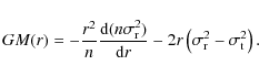
if the number density profile n(r) is also known. Given the intrinsic velocity dispersions, the enclosed mass is
)
if the number density profile n(r) is also known. Given the intrinsic velocity dispersions, the enclosed mass is
The uniqueness of the kinematical deprojection is a strong motivation for modelling the nuclear cluster in this way. One cost is that we are not able to reproduce the gradual alignment of the velocity vectors parallel to the Galactic plane that is observed outside of
Neglecting the rotation of the cluster parallel to Galactic rotation in our analysis appears justified for two reasons. First, the actual velocity of rotation and its radial dependence is not well constrained (see discussion in Sect. 8.1). Second, the influence of rotation on the mass estimates for the central parsec will be small. Even if the rotation velocity were as high as 30 km s-1 at 1 pc, this would still be only about 30% of the velocity dispersion. Since both quantities enter the Jeans equation quadratically, the error on the enclosed mass would only be of order 10%.
7.2 Moment estimators
As a first step, we examine the moment mass estimator defined by Leonard & Merritt (1989):
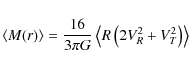
where angle brackets denote number-weighted averages over the entire system. In a cluster with constant mass-to-light ratio (i.e.,
![\begin{figure}
\par\includegraphics[angle=-90,width=8.8cm,clip]{0922fig11.eps}
\end{figure}](/articles/aa/full_html/2009/28/aa10922-08/img151.png) |
Figure 11: LM mass estimator as a function of maximum projected distance from Sgr A*, based on the proper motions in the central field. Red: late-type stars; blue: early-type stars: black: combined sample. |
| Open with DEXTER | |
Figure 11 shows the result of computing (2) as a function of the outer radius of the sample. Results from both late-type and early-type stars, considered separately, are shown; also shown is the result using the combined sample. The late-type stars alone imply a mass of ![]() 2
2 ![]()
![]() at small radii,
at small radii, ![]() pc, increasing gradually toward larger radii. The smaller sample of early-type stars yields a mass estimate that is more nearly constant with radius,
pc, increasing gradually toward larger radii. The smaller sample of early-type stars yields a mass estimate that is more nearly constant with radius,
![]()
![]()
![]() .
As noted by Paumard et al. (2006) and Lu et al. (2008), the surface number density of early-type stars
decreases steeply with distance from Sgr A*, like a power-law with index
.
As noted by Paumard et al. (2006) and Lu et al. (2008), the surface number density of early-type stars
decreases steeply with distance from Sgr A*, like a power-law with index ![]() -2. Therefore, more than
-2. Therefore, more than ![]() of the early type stars are contained within a projected radius R<0.5 pc from Sgr A*. The sample of the early-type stars can therefore be regarded as complete. The LM mass estimator for these stars at the largest projected radii can for this reason be regarded as an accurate estimate of the BH mass.
of the early type stars are contained within a projected radius R<0.5 pc from Sgr A*. The sample of the early-type stars can therefore be regarded as complete. The LM mass estimator for these stars at the largest projected radii can for this reason be regarded as an accurate estimate of the BH mass.
Estimates of
![]() based on the assumption of Keplerian motion for the closest stars to the central dark mass are generally considered to be the most reliable. For an assumed GC distance of
8.0 kpc, the most recently published values are
based on the assumption of Keplerian motion for the closest stars to the central dark mass are generally considered to be the most reliable. For an assumed GC distance of
8.0 kpc, the most recently published values are
![]()
![]() 0.6
0.6 ![]()
![]() (Ghez et al. 2003), 4.1
(Ghez et al. 2003), 4.1 ![]() 0.4
0.4 ![]()
![]() (Eisenhauer et al. 2005), 3.7
(Eisenhauer et al. 2005), 3.7 ![]() 0.2
0.2 ![]()
![]() (Ghez et al. 2005),
4.1
(Ghez et al. 2005),
4.1 ![]() 0.1
0.1 ![]()
![]() (Ghez et al. 2008), and 4.0
(Ghez et al. 2008), and 4.0 ![]() 0.1
0.1 ![]()
![]() (Gillessen et al. 2009). The value 4.0
(Gillessen et al. 2009). The value 4.0 ![]()
![]() is shown as the dashed line in Fig. 11; it is consistent with the LM mass estimate derived from the young stars, but lies above the estimate derived from the old stars for
is shown as the dashed line in Fig. 11; it is consistent with the LM mass estimate derived from the young stars, but lies above the estimate derived from the old stars for ![]() pc.
pc.
The comparison is complicated by the fact that the NSC extends probably far beyond the central parsec. Samples that extend to projected distances of ![]() 1 pc from Sgr A* contain many stars that are moving far from the BH and that feel the gravitational force from the distributed mass. The gradual rise in
1 pc from Sgr A* contain many stars that are moving far from the BH and that feel the gravitational force from the distributed mass. The gradual rise in
![]() at
at ![]() pc - in contrast to the near constant LM mass estimator for the early-type stars - may reflect this. On the other hand, restricting the sample to small projected radii is inconsistent with the assumptions made in deriving the LM estimator and will also bias the estimate.
pc - in contrast to the near constant LM mass estimator for the early-type stars - may reflect this. On the other hand, restricting the sample to small projected radii is inconsistent with the assumptions made in deriving the LM estimator and will also bias the estimate.
We note that many previous studies based on radial velocities or proper motions of stars in the inner parsec have found values of
![]() that were
that were ![]()
![]() lower than the currently accepted value (e.g. Ghez et al. 1998; Genzel et al. 2000; Eckart & Genzel 1997; Chakrabarty & Saha 2001). Figer et al. (2003) and Zhu et al. (2008) have argued that this bias can be attributed to the low space density of late-type stars near Sgr A*. Indeed there appears to be a ``hole'' in the distribution of old stars: their number counts are flat inside of
lower than the currently accepted value (e.g. Ghez et al. 1998; Genzel et al. 2000; Eckart & Genzel 1997; Chakrabarty & Saha 2001). Figer et al. (2003) and Zhu et al. (2008) have argued that this bias can be attributed to the low space density of late-type stars near Sgr A*. Indeed there appears to be a ``hole'' in the distribution of old stars: their number counts are flat inside of ![]() 0.25 pc, implying a space density that may even decline toward Sgr A* (Zhu et al. 2008, and discussion therein). In the extreme case of
no stars intrinsically close to the BH, mass estimates based on the moment equations would clearly be biased toward low values. The drop of the LM mass estimate for the late-type stars
down to only about 50% of the actual BH mass is most probably related to this deficit which leads to an underestimation of the true 3D distances of the stars from Sgr A*. The fact that the
proper motion velocity dispersions of the dominant (late-type) population are observed to rise toward the projected center (e.g. Fig. 6) suggests that at least some of the
old stars are physically close to the BH. Nevertheless, Fig. 11 reinforces the idea that estimates of the BH mass from proper motions might be significantly influenced by the spatial
distribution of the kinematical sample.
0.25 pc, implying a space density that may even decline toward Sgr A* (Zhu et al. 2008, and discussion therein). In the extreme case of
no stars intrinsically close to the BH, mass estimates based on the moment equations would clearly be biased toward low values. The drop of the LM mass estimate for the late-type stars
down to only about 50% of the actual BH mass is most probably related to this deficit which leads to an underestimation of the true 3D distances of the stars from Sgr A*. The fact that the
proper motion velocity dispersions of the dominant (late-type) population are observed to rise toward the projected center (e.g. Fig. 6) suggests that at least some of the
old stars are physically close to the BH. Nevertheless, Fig. 11 reinforces the idea that estimates of the BH mass from proper motions might be significantly influenced by the spatial
distribution of the kinematical sample.
7.3 Isotropic modelling
Proper motion velocities of the late-type stars appear to be nearly isotropic at most radii (Fig. 6). As our next step, we therefore model the NSC assuming
![]() at all radii. Writing
at all radii. Writing
![]() ,
it is easy to show (e.g. Genzel et al. 1996) that
,
it is easy to show (e.g. Genzel et al. 1996) that
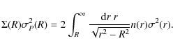
Here
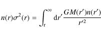
and combining (3) and (4),
| |
= | 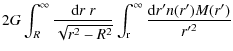 |
(5) |
| = | 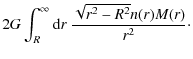 |
(6) |
Finally, writing
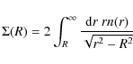 |
(7) |
yields
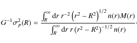
The simplest case to consider is a model in which all of the mass is in the central black hole,
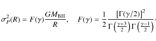 |
(9) |
The function F is weakly dependent on
![\begin{figure}
\par\includegraphics[angle=-90,width=8.8cm,clip]{0922fig12.eps}
\end{figure}](/articles/aa/full_html/2009/28/aa10922-08/img179.png) |
Figure 12:
Modelling the nuclear cluster assuming that all the mass is contained in the black hole and that the velocities are isotropic. The number density profile of the kinematical sample was assumed to be a single power law of the radius. Open circles are velocity dispersions computed using fixed radial bins; blue points are absolute values of the measured velocities. Straight lines show model predictions for
|
| Open with DEXTER | |
Continuing under the assumption of isotropy, we can constrain a model of the stellar mass density by comparing the predictions of Eq. (8) with the observed velocities via
![\begin{displaymath}%
\chi^2 =
\sum_{i=1}^N {\left[V_i^2-\sigma_P^2(R_i)\right]^2\over
\Delta^2(R_i)}
\end{displaymath}](/articles/aa/full_html/2009/28/aa10922-08/img180.png)
under various assumptions about M(r). Here, N is the number of measured velocities,
We minimized ![]() over a set of parameters defining the mass distribution:
over a set of parameters defining the mass distribution:
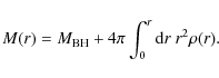 |
(11) |
If we assume simple power laws for both n(r) and
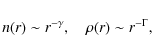 |
(12) |
the integral in the numerator of Eq. (8) is divergent unless
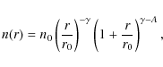
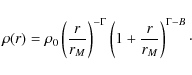
A number of studies have found a large-radius (
For the mass density ![]() we set rM=5 pc
we set rM=5 pc ![]() 100'' and B=4, yielding essentially a single power-law dependence,
100'' and B=4, yielding essentially a single power-law dependence,
![]() ,
over the radial range of our data.
For a given n(r), the three remaining parameters are the BH mass, the mass density slope
,
over the radial range of our data.
For a given n(r), the three remaining parameters are the BH mass, the mass density slope ![]() ,
and the mass density normalization
,
and the mass density normalization ![]() .
These can be written
.
These can be written
| (15) |
where
![\begin{figure}
\par\includegraphics[angle=-90,width=8.8cm,clip]{0922fig13.eps}
\end{figure}](/articles/aa/full_html/2009/28/aa10922-08/img201.png) |
Figure 13:
Isotropic modelling of the nuclear cluster including a contribution to the gravitational potential from the stars, assumed to have a mass density that falls off
as
|
| Open with DEXTER | |
Figure 13 illustrates the effects of including a non-zero stellar mass. Each model shown there has
![]()
![]()
![]() and
and ![]() ,
i.e. the stellar mass density falls as
,
i.e. the stellar mass density falls as ![]() r-1 in the region where there are velocity data. The best fit from this series is obtained for
r-1 in the region where there are velocity data. The best fit from this series is obtained for
![]()
![]()
![]()
![]() .
Because the central slope of n(r) (
.
Because the central slope of n(r) (
![]() )
is flatter than was assumed for Fig. 12 (
)
is flatter than was assumed for Fig. 12 (
![]() ), the observable effect of the BH on the stellar motions near the projected
center is smaller and a more massive BH is required to reproduce the inner velocity dispersions.
), the observable effect of the BH on the stellar motions near the projected
center is smaller and a more massive BH is required to reproduce the inner velocity dispersions.
Figure 14 summarizes the fits of a set of mass models computed on a 3d grid in parameter space. For each (
![]() ), the plot shows contours of two quantities associated with the model that best fits the kinematical data:
), the plot shows contours of two quantities associated with the model that best fits the kinematical data:
![]()
![]() and
and ![]() .
The red (dashed) contours show confidence intervals of 68%, 90%, and 99% (Lampton et al. 1976). The overall best-fit model from this set has a negative
.
The red (dashed) contours show confidence intervals of 68%, 90%, and 99% (Lampton et al. 1976). The overall best-fit model from this set has a negative ![]() ,
i.e., the mass density increases with radius. However the value of
,
i.e., the mass density increases with radius. However the value of ![]() is very weakly constrained, especially if
is very weakly constrained, especially if
![]() is considered to be a free parameter. Moving up along the near-plateau in
is considered to be a free parameter. Moving up along the near-plateau in ![]() ,
a decreasing BH mass can be compensated for by increasing the stellar mass and by making the mass density profile more steep, mimicking a central point mass. Figure 15 plots the minimum
,
a decreasing BH mass can be compensated for by increasing the stellar mass and by making the mass density profile more steep, mimicking a central point mass. Figure 15 plots the minimum ![]() value at each
value at each
![]() .
The ``correct'' BH mass, 4.0
.
The ``correct'' BH mass, 4.0 ![]()
![]() ,
is consistent at the 90% level with the isotropic modelling.
,
is consistent at the 90% level with the isotropic modelling.
![\begin{figure}
\par\includegraphics[angle=-90,width=8.2cm,clip]{0922fig14.eps}
\end{figure}](/articles/aa/full_html/2009/28/aa10922-08/img206.png) |
Figure 14:
Results of isotropic modelling of the NSC assuming the mass model of Eq. (14). The three parameters (
|
| Open with DEXTER | |
![\begin{figure}
\par\includegraphics[angle=-90,width=8cm,clip]{0922fig15.eps}
\end{figure}](/articles/aa/full_html/2009/28/aa10922-08/img207.png) |
Figure 15:
|
| Open with DEXTER | |
The best-fitting isotropic models all require a non-zero distributed mass. If ![]() is assumed to decrease with radius, i.e.
is assumed to decrease with radius, i.e. ![]() ,
then the implied mass within 1 pc is always greater than
,
then the implied mass within 1 pc is always greater than ![]() 0.4
0.4 ![]()
![]() for 3.5
for 3.5 ![]()
![]()
![]() 106. If
106. If
![]()
![]()
![]() and
and ![]() ,
the distributed mass within 1 pc must be greater than
,
the distributed mass within 1 pc must be greater than ![]() 0.5
0.5 ![]()
![]() .
.
7.4 Anisotropic modelling
We next consider models that allow the two independent components (
![]() )
of the stellar velocity dispersion to be different at each intrinsic radius r. In principle, complete knowledge of the two proper-motion velocity dispersion profiles
)
of the stellar velocity dispersion to be different at each intrinsic radius r. In principle, complete knowledge of the two proper-motion velocity dispersion profiles
![]() ,
together with the deprojected number-density profile n(r),
is equivalent to complete knowledge of
,
together with the deprojected number-density profile n(r),
is equivalent to complete knowledge of
![]() and
and
![]() (Leonard & Merritt 1989). The enclosed mass would then follow uniquely from the Jeans equation.
In practice, we only measure the proper motions over a limited range of radii, and inferences about the mass density will in general depend on the degree of anisotropy beyond the last
measured point (e.g. Merritt 1988). In addition, as discussed above, the assumption of spherical symmetry in the modelling is not completely consistent with the observed behavior of the proper motions at large radii. For these reasons, a direct deprojection of the proper-motion
velocity dispersions was deemed undesirable. Instead we constructed anisotropic models and compared their projected properties with the data. We stress that our algorithm is completely nonparametric in terms of its treatment of
(Leonard & Merritt 1989). The enclosed mass would then follow uniquely from the Jeans equation.
In practice, we only measure the proper motions over a limited range of radii, and inferences about the mass density will in general depend on the degree of anisotropy beyond the last
measured point (e.g. Merritt 1988). In addition, as discussed above, the assumption of spherical symmetry in the modelling is not completely consistent with the observed behavior of the proper motions at large radii. For these reasons, a direct deprojection of the proper-motion
velocity dispersions was deemed undesirable. Instead we constructed anisotropic models and compared their projected properties with the data. We stress that our algorithm is completely nonparametric in terms of its treatment of
![]() and
and
![]() .
.
The relation between the intrinsic and projected velocity dispersions is
![$\displaystyle %
\Sigma(R)\sigma_R^2(R) = 2\int_R^{R_{\rm max}} {r {\rm d}r\over...
...gma_{\rm r}^2(r)
+ \left(1-{R^2\over r^2}\right) n(r)\sigma_{\rm t}^2(r)\bigg],$](/articles/aa/full_html/2009/28/aa10922-08/img212.png)
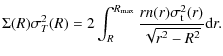
We chose as our undetermined function

Because f(r) appears as a derivative in this expression, we needed to impose a constraint to ensure that f remains a smooth differentiable function during the optimization. We did this in the standard way by adding a penalty function to
![\begin{displaymath}%
P_\lambda(n\sigma_{\rm r}^2) =
\lambda \int_0^{\infty} \left[{{\rm d}^2\log f\over {\rm d}\log r^2}\right]^2 {\rm d}r
\end{displaymath}](/articles/aa/full_html/2009/28/aa10922-08/img217.png)
with
The goodness of fit of the model to the data was defined in a manner analogous to the isotropic case:
![\begin{displaymath}%
\chi^2 =
\sum_{i=1}^N {\left[V_{R,i}^2-\sigma_R^2(R_i)\rig...
..._{T,i}^2-\sigma_T^2(R_i)\right]^2\over
\Delta_T^2(R_i^2)}\cdot
\end{displaymath}](/articles/aa/full_html/2009/28/aa10922-08/img222.png)
In this expression, the functions
The radial grid on which
![]() was specified extended to 50 pc, well beyond the outermost measured velocity at
was specified extended to 50 pc, well beyond the outermost measured velocity at ![]() 1 pc. It was discovered that allowing complete freedom in
1 pc. It was discovered that allowing complete freedom in
![]() in the region
in the region
![]() led sometimes to solutions
in which the anisotropy was very large and/or increasing at large radii. Such models reproduce the observed departures from a Keplerian velocity falloff at
led sometimes to solutions
in which the anisotropy was very large and/or increasing at large radii. Such models reproduce the observed departures from a Keplerian velocity falloff at ![]() 1 pc by placing stars on very eccentric orbits beyond the region where the solution is strongly constrained by the data.
While such models are physically permissible, they seem rather unlikely. We focus here on models that were constrained at large radii to be isotropic. Specifically, we forced
1 pc by placing stars on very eccentric orbits beyond the region where the solution is strongly constrained by the data.
While such models are physically permissible, they seem rather unlikely. We focus here on models that were constrained at large radii to be isotropic. Specifically, we forced
![]() to be equal to the isotropic
to be equal to the isotropic ![]() ,
Eq. (4), at all
,
Eq. (4), at all
![]() .
Imposing this constraint (which results in a different
.
Imposing this constraint (which results in a different
![]() profile at
profile at
![]() pc for each assumed M(r)) guarantees that
pc for each assumed M(r)) guarantees that
![]() at
at
![]() .
.
The results are summarized in Figs. 16-19. Overall the results are
similar to those obtained under the assumption of isotropy, except that the confidence intervals are somewhat narrower, due to the additional information contained within the two velocity dispersion
components. The 90% confidence bounds on
![]() (Fig. 17) are 3.1
(Fig. 17) are 3.1 ![]()
![]()
![]()
![]() .
.
Figure 18 shows the kinematics of the best-fit solution, with
![]()
![]()
![]() .
The stellar velocities are mildly radially anisotropic at
.
The stellar velocities are mildly radially anisotropic at ![]() pc
and mildly tangentially anisotropic for
pc
and mildly tangentially anisotropic for
![]() pc; by construction, they are isotropic beyond
pc; by construction, they are isotropic beyond ![]() 3 pc.
3 pc.
Figure 19 shows the kinematics of a second solution with
![]()
![]()
![]() and
and ![]() ;
the stellar mass within 1 pc is 0.5
;
the stellar mass within 1 pc is 0.5 ![]()
![]() .
The differences with the global best-fit model are slight, consisting mostly of a higher degree of anisotropy.
.
The differences with the global best-fit model are slight, consisting mostly of a higher degree of anisotropy.
We note that both the isotropic and anisotropic modelling seem to rule out securely a mass density profile as steep as
![]() .
.
![\begin{figure}
\par\includegraphics[angle=-90,width=8cm,clip]{0922fig16.eps}
\end{figure}](/articles/aa/full_html/2009/28/aa10922-08/img235.png) |
Figure 16: Like Fig. 14, but for the anisotropic modelling. |
| Open with DEXTER | |
![\begin{figure}
\par\includegraphics[angle=-90,width=8cm,clip]{0922fig17.eps}
\end{figure}](/articles/aa/full_html/2009/28/aa10922-08/img236.png) |
Figure 17: Like Fig. 15 but for the anisotropic modelling. |
| Open with DEXTER | |
![\begin{figure}
\par\includegraphics[width=8.8cm,clip]{0922fig18.eps}
\end{figure}](/articles/aa/full_html/2009/28/aa10922-08/img237.png) |
Figure 18: Best-fit anisotropic model. a) and b) are the projected, radial and tangential velocity dispersions (black/solid lines), compared with a kernel-based velocity dispersion profile and associated (90%, 95%, 98%) confidence intervals (blue/dashed lines). c) Intrinsic velocity dispersions: radial (solid) and tangential (dashed) lines. |
| Open with DEXTER | |
![\begin{figure}
\par\includegraphics[width=8.8cm,clip]{0922fig19.eps}
\end{figure}](/articles/aa/full_html/2009/28/aa10922-08/img239.png) |
Figure 19:
Anisotropic model with
|
| Open with DEXTER | |
8 Discussion
8.1 Rotation of the NSC
![\begin{figure}
\par\includegraphics[width=9cm,clip]{0922fig20.eps}
\end{figure}](/articles/aa/full_html/2009/28/aa10922-08/img240.png) |
Figure 20: Line-of-sight velocity vs. Galactic longitude. Blue circles: measurements from McGinn et al. (1989); green stars: measurements from Trippe et al. (2008). The straight orange line indicates the model of Trippe et al. (2008). The dashed black ellipses show the data that are not shown in Fig. 12 of Trippe et al. (2008). |
| Open with DEXTER | |
An early spectroscopic study by McGinn et al. (1989) found evidence for rotation of the GC NSC, at least beyond 1 pc distance from Sgr A*. Other earlier studies based on spectroscopic observations have found no signs of net rotation in the late-type stars in the nuclear star cluster (Genzel et al. 2000; Sellgren et al. 1990; Figer et al. 2003, the latter present a detailed analysis). However, these studies were based on small numbers of late-type stars in the central parsec of the Milky Way and did therefore probably not reach the necessary accuracy of a few km s-1 needed to detect rotation in the innermost parsec.
Trippe et al. (2008) found clear signs for an overall rotation of the NSC parallel to galactic rotation through the analysis of proper motions and new adaptive-optics assisted integral field spectroscopic observations. The results of our work confirm their finding of an overall rotation of the NSC in the Galactic. Trippe et al. (2008) provide a model for the rotation velocity that increases linearly with Galactic longitude with a value of 1.42 ![]() 0.36 km s-1 per
arcsecond projected distance from Sgr A* along Galactic longitude.
0.36 km s-1 per
arcsecond projected distance from Sgr A* along Galactic longitude.
We show the data of McGinn et al. (1989) and Trippe et al. (2008) in Fig. 20. Figure 20 includes all data from McGinn et al. (1989). For unknown reasons,
Trippe et al. (2008) only show 5 of 17 data points of McGinn et al. (1989). The plot shows that while the model of Trippe et al. (2008) fits well all the data in the central few tens of arcseconds, the rotation curve may be considerably flatter at Galactic longitudes
![]() .
Due to the strong and highly variable extinction toward the GC, the data of McGinn et al. (1989)
may sample quite different depths and therefore stellar populations. We may therefore speculate on the possibility that we actually see two distinct rotating systems in the GC, one with a steeper and one with a flatter rotation curve. In this context it appears worthwhile to point out the recent result of Seth et al. (2008b) from integral-field spectroscopy of the nuclear star cluster of NGC 4244: they identify a younger disk-like stellar population superposed on an
older spheroidal component. It may be that a similar situation presents itself in the center of the Milky Way. A nuclear disk exists the GC in addition to the spherical NSC by Launhardt et al. (2002). However, an important caveat is the fact that the size scale of the nuclear disk is orders of magnitudes larger than the one of the NSC, unlike the situation in NGC 4244.
.
Due to the strong and highly variable extinction toward the GC, the data of McGinn et al. (1989)
may sample quite different depths and therefore stellar populations. We may therefore speculate on the possibility that we actually see two distinct rotating systems in the GC, one with a steeper and one with a flatter rotation curve. In this context it appears worthwhile to point out the recent result of Seth et al. (2008b) from integral-field spectroscopy of the nuclear star cluster of NGC 4244: they identify a younger disk-like stellar population superposed on an
older spheroidal component. It may be that a similar situation presents itself in the center of the Milky Way. A nuclear disk exists the GC in addition to the spherical NSC by Launhardt et al. (2002). However, an important caveat is the fact that the size scale of the nuclear disk is orders of magnitudes larger than the one of the NSC, unlike the situation in NGC 4244.
As pointed out by Seth et al. (2008b), rotation of the NSC parallel to Galactic rotation implies that it may at least in part have formed by accretion of gas or star clusters from the galactic disk. This is of great importance for understanding the origin of nuclear star clusters in galaxies (for a brief overview of some formation scenarios see, e.g., Böker 2008).
8.2 Isotropy/anisotropy
Consistent with earlier work (e.g. Genzel et al. 2000) we find evidence for tangential mean motion in the central arcseconds (see Fig. 4). This anisotropy is related to the presence of young, massive stars, a significant fraction of which shows coherent motion within one (or possibly two) stellar disks (Genzel et al. 2003; Lu et al. 2006; Paumard et al. 2006; Levin & Beloborodov 2003). Lu et al. (2008) discard the existence of the counter-clockwise disk and show that about 50% of the young stars belong to the clockwise rotating disk, while the other 50% appear to have more randomized motions. Our analysis here shows that, after excluding the early-type stars, the cluster appears close to isotropic (see lower left panel in Fig. 6, right panel in Fig. 10, and left panel in Fig. B.3). The situation may be different in the innermost 6'', where the data are somewhat more ambiguous (see lower left panel of Fig. 6). Our anisotropic Jeans models also result in solutions are are close to isotropy (see Figs. 18 and 19). A caveat is, however, the rotation of the cluster, which could mask anisotropy with a signature smaller than or comparable to the rotation signature.
8.3 Mass modeling: black hole mass
Our modeling of the proper motion data yields a best-fit black hole mass of
3.6+0.2-0.4 ![]()
![]() (68%) under the isotropic assumption, and
3.5+0.15-0.35
(68%) under the isotropic assumption, and
3.5+0.15-0.35 ![]()
![]() if anisotropy is allowed (for an assumed distance of 8 kpc to the GC). The smaller uncertainties of the anisotropic model may appear counter-intuitive. However, when we go from isotropic to anisotropic models, we also go from one observed function (the isotropized velocity dispersion profile) to two observed functions (the two,
radial and tangential dispersion profiles). So from a mathematical point of view, the ratio between the number of ``model functions'' and the number of ``data functions'' remains the same. There is no obvious reason why the error bars on BH mass obtained from the isotropic modelling should be tighter, or looser, than those obtained from the anisotropic modelling.
if anisotropy is allowed (for an assumed distance of 8 kpc to the GC). The smaller uncertainties of the anisotropic model may appear counter-intuitive. However, when we go from isotropic to anisotropic models, we also go from one observed function (the isotropized velocity dispersion profile) to two observed functions (the two,
radial and tangential dispersion profiles). So from a mathematical point of view, the ratio between the number of ``model functions'' and the number of ``data functions'' remains the same. There is no obvious reason why the error bars on BH mass obtained from the isotropic modelling should be tighter, or looser, than those obtained from the anisotropic modelling.
A BH mass of 4.0 ![]()
![]() is consistent with the modelling at the 90% (isotropic) and 99% (anisotropic) levels. Thus, while a value for
is consistent with the modelling at the 90% (isotropic) and 99% (anisotropic) levels. Thus, while a value for
![]() slightly lower than the currently canonical value (Ghez et al. 2003,2008; Eisenhauer et al. 2005; Ghez et al. 2005) is
preferred by our modelling, our results are still consistent with that value.
slightly lower than the currently canonical value (Ghez et al. 2003,2008; Eisenhauer et al. 2005; Ghez et al. 2005) is
preferred by our modelling, our results are still consistent with that value.
Mass estimates of Sgr A* based on proper motions (e.g. Genzel et al. 2000; Ghez et al. 1998; Chakrabarty & Saha 2001; Eckart et al. 2002) have routinely provided lower values than what has been found by the analysis of stellar orbits. The orbit of the star S2/S0-2 has consistently provided higher black hole masses with high precision (see above). Determining the mass of Sgr A* from a stellar orbit is straightforward and relies solely on the assumption that the star moves on a Keplerian orbit and that higher order effects can be neglected (see, e.g., Weinberg et al. 2005; Zucker et al. 2006; Ghez et al. 2008; Rubilar & Eckart 2001, and others). Mass estimates based on proper motions, on the other hand, have to make a number of assumptions on the spatial and velocity structure of the cluster that can bias the results.
Source confusion and the fast proper motion of stars within
![]() pc of Sgr A* may have biased the proper motions of stars near Sgr A* in early work (e.g., Genzel et al. 2000,1997; Ghez et al. 1998) toward lower values of the velocity dispersion (identification of slow stars is easier between epochs; faint and fast stars become easily confused with brighter ones). In this work, we only use high-resolution AO observations at an 8 m-class telescope. The bias toward low velocity dispersion therefore should be minimal. Also, the modeling uses proper motions in the entire central parsec. This decreases considerably the
weight of the possibly biased proper motions within
pc of Sgr A* may have biased the proper motions of stars near Sgr A* in early work (e.g., Genzel et al. 2000,1997; Ghez et al. 1998) toward lower values of the velocity dispersion (identification of slow stars is easier between epochs; faint and fast stars become easily confused with brighter ones). In this work, we only use high-resolution AO observations at an 8 m-class telescope. The bias toward low velocity dispersion therefore should be minimal. Also, the modeling uses proper motions in the entire central parsec. This decreases considerably the
weight of the possibly biased proper motions within
![]() .
.
The black hole masses from both our isotropic and anisotropic models are in reasonable agreement with the measurements from the orbit of S2/S0-2. We believe that the most important source of bias for the determination of the BH mass from proper motions is the assumed law for the radial dependence of the tracer population from distance to Sgr A*. Earlier work has usually assumed steep power-laws (e.g.,
![]() in Genzel et al. 2000) for the tracer population. This leads inevitably to an under-estimation of the 3D distances of the tracer stars from the BH because the number density behaves rather like
in Genzel et al. 2000) for the tracer population. This leads inevitably to an under-estimation of the 3D distances of the tracer stars from the BH because the number density behaves rather like
![]() in the central parsec (Schödel et al. 2007). The issue becomes even more important when the analysis is limited to the late-type stars near Sgr A*, whose density may be even decreasing toward the black hole (see, e.g.,
Figer et al. 2003; Genzel et al. 2003; Buchholz et al. 2009). In our analysis we have assumed
in the central parsec (Schödel et al. 2007). The issue becomes even more important when the analysis is limited to the late-type stars near Sgr A*, whose density may be even decreasing toward the black hole (see, e.g.,
Figer et al. 2003; Genzel et al. 2003; Buchholz et al. 2009). In our analysis we have assumed
![]() for the late-type stars near Sgr A*. This is the flattest power-law still consistent with isotropy. The issue is worth further investigation.
for the late-type stars near Sgr A*. This is the flattest power-law still consistent with isotropy. The issue is worth further investigation.
8.4 Mass modeling: cluster mass
Our basic modeling assumptions are stationarity and spherical symmetry of the cluster. We show that the proper motion data cannot be explained by just a point mass at the position of Sgr A*. Both isotropic and anisotropic Jeans models require a mass within ![]() pc of >0.5
pc of >0.5 ![]()
![]() ,
in addition to the point mass of the black hole, Sgr A* (under the assumption that
,
in addition to the point mass of the black hole, Sgr A* (under the assumption that ![]() ,
i.e. the mass density increases toward Sgr A*). Also, the Leonard Merritt moment mass estimator shows clear evidence for an increasing contribution of extended/stellar mass
to the gravitational potential at
,
i.e. the mass density increases toward Sgr A*). Also, the Leonard Merritt moment mass estimator shows clear evidence for an increasing contribution of extended/stellar mass
to the gravitational potential at ![]() pc. The result for the amount of extended mass within r=1 pc is insensitive to the exact assumed density-law for the tracer population in the immediate
vicinity of Sgr A* (see above).
pc. The result for the amount of extended mass within r=1 pc is insensitive to the exact assumed density-law for the tracer population in the immediate
vicinity of Sgr A* (see above).
As an alternative to the assumptions made above, we can model the proper motions assuming that the stellar mass density is proportional to the stellar number density, Eq. (13), and that the mass of the black hole is the value given by modelling of the S-star orbits, 4.0 ![]()
![]() .
The single remaining free parameter is then the normalization of the stellar mass density, i.e, the mass-to-light ratio of the stars. Figure 21 shows how the fit to the proper motion data varies as a function of the stellar mass under these assumptions, for both isotropic and anisotropic cases. The preferred value for the stellar mass within 1 pc is seen to be
.
The single remaining free parameter is then the normalization of the stellar mass density, i.e, the mass-to-light ratio of the stars. Figure 21 shows how the fit to the proper motion data varies as a function of the stellar mass under these assumptions, for both isotropic and anisotropic cases. The preferred value for the stellar mass within 1 pc is seen to be
![]() 1.5
1.5 ![]()
![]() (isotropic) and
(isotropic) and ![]() 1.1
1.1 ![]()
![]() (anisotropic).
(anisotropic).
![\begin{figure}
\par\includegraphics[width=9cm,clip]{0922fig21.eps}
\end{figure}](/articles/aa/full_html/2009/28/aa10922-08/img249.png) |
Figure 21:
Fits to the proper motion data when the BH mass is fixed to 4.0 |
| Open with DEXTER | |
While early work (e.g., Eckart et al. 1993; Sellgren et al. 1990) found enclosed masses at
![]() pc that are comparable to what we have derived in this work, almost negligible amounts of extended, i.e. stellar, mass within R<1 pc were reported in later work (see,e.g., Schödel et al. 2003; Genzel et al. 2000; Haller et al. 1996). However, with these low values it would be difficult to reconcile the high mass of the NSC of 3.5
pc that are comparable to what we have derived in this work, almost negligible amounts of extended, i.e. stellar, mass within R<1 pc were reported in later work (see,e.g., Schödel et al. 2003; Genzel et al. 2000; Haller et al. 1996). However, with these low values it would be difficult to reconcile the high mass of the NSC of 3.5 ![]() 1.5
1.5 ![]()
![]() (Launhardt et al. 2002) with the almost zero mass in the central
parsec: the old mass models would not reach the integrated mass of the NSC within its radius of
(Launhardt et al. 2002) with the almost zero mass in the central
parsec: the old mass models would not reach the integrated mass of the NSC within its radius of ![]() 10 pc. High precision measurements of the velocity of the maser star IRS 9, located at R=0.33 pc may also indicate an enclosed mass of a few times
10 pc. High precision measurements of the velocity of the maser star IRS 9, located at R=0.33 pc may also indicate an enclosed mass of a few times
![]() in addition to the mass of Sgr A* (Reid et al. 2007). Schödel et al. (2007) have roughly estimated the enclosed extended mass in the central parsec by combining the measured line-of-sight velocity dispersion of late-type stars in the central pc, assuming isotropy, with the derived density structure of
the stellar cluster. They found that the enclosed mass in the GC may start to rise significantly already at projected distances from Sgr A* as low as
in addition to the mass of Sgr A* (Reid et al. 2007). Schödel et al. (2007) have roughly estimated the enclosed extended mass in the central parsec by combining the measured line-of-sight velocity dispersion of late-type stars in the central pc, assuming isotropy, with the derived density structure of
the stellar cluster. They found that the enclosed mass in the GC may start to rise significantly already at projected distances from Sgr A* as low as
![]() pc.
pc.
What can be the reason why the enclosed stellar mass at the GC has been underestimated in the past decade? We believe that there are primarily two factors responsible. In the absence of adequately sampled proper motion or line-of-sight velocity measurements at distances ![]() pc, it was necessary to include measurements of gas velocities in the circum nuclear disk (e.g., Christopher et al. 2005; Guesten et al. 1987) into the mass estimates. However, gas can be subject to winds, magnetic fields, or cloud collisions, contrary to stars, which are ideal test particles of the gravitational potential. A second factor that influenced previous mass estimates of the stellar cluster around Sgr A* were model assumptions and the related combination data sets within a too simple model (just a bulge, no NSC, no nuclear disk). In principle, earlier assumptions ignored the existence of the MW NSC. The effect was to include bulge velocity dispersions into the mass estimates (Haller et al. 1996), e.g., include measurements at distances of
pc, it was necessary to include measurements of gas velocities in the circum nuclear disk (e.g., Christopher et al. 2005; Guesten et al. 1987) into the mass estimates. However, gas can be subject to winds, magnetic fields, or cloud collisions, contrary to stars, which are ideal test particles of the gravitational potential. A second factor that influenced previous mass estimates of the stellar cluster around Sgr A* were model assumptions and the related combination data sets within a too simple model (just a bulge, no NSC, no nuclear disk). In principle, earlier assumptions ignored the existence of the MW NSC. The effect was to include bulge velocity dispersions into the mass estimates (Haller et al. 1996), e.g., include measurements at distances of ![]() 100 pc from Sgr A* into their analysis, while Genzel et al. (1996) assume
100 pc from Sgr A* into their analysis, while Genzel et al. (1996) assume
![]() km s-1 in their Jeans modelling. However, the velocity dispersion of the Milky Way bulge is fairly uncertain (see Merritt & Ferrarese 2001; Tremaine et al. 2002). Also, the MW NSC may well be a system that is dynamically decoupled from the bulge.
km s-1 in their Jeans modelling. However, the velocity dispersion of the Milky Way bulge is fairly uncertain (see Merritt & Ferrarese 2001; Tremaine et al. 2002). Also, the MW NSC may well be a system that is dynamically decoupled from the bulge.
As described in the introduction, observations in the 1990s (mainly by HST) revealed the existence of nuclear star clusters as entities that are morphologically and dynamically separate from the bulges. This cannot be neglected in the determination of the MW NSC mass. If the velocity dispersion in the bulge is lower than in the NSC, then spectroscopically measured velocity dispersions outside of the central parsec may already be biased toward low values (due to superposition of bulge stars along the line of sight toward the NSC). This may be the reason why Rieke & Rieke (1988) obtain a line-of-sight velocity dispersion from late type stars in the region
0.36<R<6.5 pc (![]() km s-1) that is lower than the
km s-1) that is lower than the
![]() km s-1 for late-type stars within R<0.8 pc measured by Genzel et al. (2000), Figer et al. (2003),
or Zhu et al. (2008).
km s-1 for late-type stars within R<0.8 pc measured by Genzel et al. (2000), Figer et al. (2003),
or Zhu et al. (2008).
What are the consequences of the - compared to previously published values - significantly increased stellar mass in the cluster around Sgr A*? As concerns theoretical models of the dynamics of gas and stars at the GC, future modelling must take into account that the gravitational potential at the GC starts deviating from that of a point mass significantly already at a distance of roughly 0.5 pc from Sgr A*. As pointed out by Schödel et al. (2007) an important implication of the non-negligible mass of the NSC implies that the CND cannot be modeled as a simple disk in Keplerian rotation. This is also supported by the mass models of Figer et al. (2003). Also, the
dynamics of the mini-spiral (see Lacy et al. 1991; Vollmer & Duschl 2000; Paumard et al. 2004) will
probably have to be revised (also to take into account the ![]()
![]() increased black hole mass, compared to the values used in some of these models).
increased black hole mass, compared to the values used in some of these models).
Our models do not allow us to set strong constraints on the power-law index of the assumed mass distribution. Assuming increasing mass density toward the black hole, values of
![]() can be reconciled with the models. The power-law index of the stellar density profile reported by Schödel et al. (2007) is 1.19
can be reconciled with the models. The power-law index of the stellar density profile reported by Schödel et al. (2007) is 1.19 ![]() 0.05 in the central parsec. This value lies within the range of the
0.05 in the central parsec. This value lies within the range of the ![]() -values from our models. A caveat at this point is, however, that Schödel et al. (2007) did not explicitly discard early-type stars from their number counts and therefore report some sort of average value for early and late-type populations. When only the
late-type stars are considered, the density profile may be considerably flatter or even slightly inverted in the immediate environment of Sgr A* (see,e.g., Genzel et al. 2003; Figer et al. 2003, or Buchholz et al. 2009). The exact density profile of the late-type stars is an important issue that needs to be addressed by future research.
-values from our models. A caveat at this point is, however, that Schödel et al. (2007) did not explicitly discard early-type stars from their number counts and therefore report some sort of average value for early and late-type populations. When only the
late-type stars are considered, the density profile may be considerably flatter or even slightly inverted in the immediate environment of Sgr A* (see,e.g., Genzel et al. 2003; Figer et al. 2003, or Buchholz et al. 2009). The exact density profile of the late-type stars is an important issue that needs to be addressed by future research.
A value as high as
![]() in the central parsec appears to be safely ruled out (Figs. 14 and 16). The parameter
in the central parsec appears to be safely ruled out (Figs. 14 and 16). The parameter ![]() is of great importance because it determines the radial profile of the mass density. The latter has important consequences for stellar dynamics because the high densities shorten the relaxation time and increase the probability for close stellar encounters or collisions. There may be a non-negligible probability of
stellar collisions at radii r<0.2 pc during the lifetimes of stars, causing - among other effects - the destruction of the envelopes of giant stars (see Freitag et al. 2008; Alexander 2003). The derived collision probabilities presented in Freitag et al. (2008) are observationally supported by the distinct lack of late-type (giant)
stars within
is of great importance because it determines the radial profile of the mass density. The latter has important consequences for stellar dynamics because the high densities shorten the relaxation time and increase the probability for close stellar encounters or collisions. There may be a non-negligible probability of
stellar collisions at radii r<0.2 pc during the lifetimes of stars, causing - among other effects - the destruction of the envelopes of giant stars (see Freitag et al. 2008; Alexander 2003). The derived collision probabilities presented in Freitag et al. (2008) are observationally supported by the distinct lack of late-type (giant)
stars within
![]() of Sgr A* (see Zhu et al. 2008; Genzel et al. 2003; Haller et al. 1996; Figer et al. 2003; Genzel et al. 1996). The collision rates reported by Freitag et al. (2008) are based on steep (
of Sgr A* (see Zhu et al. 2008; Genzel et al. 2003; Haller et al. 1996; Figer et al. 2003; Genzel et al. 1996). The collision rates reported by Freitag et al. (2008) are based on steep (
![]() )
density profiles. While such a steep profile is not excluded by our analysis and the mass densities of
)
density profiles. While such a steep profile is not excluded by our analysis and the mass densities of
![]()
![]() pc-3 required by the models of Freitag et al. may be consistent with our estimates, it is nevertheless important to note that flatter mass profiles are preferred by our
Jeans modeling. Also, the profiles derived from stellar number counts suggest rather shallow profiles near Sgr A* (see above).
pc-3 required by the models of Freitag et al. may be consistent with our estimates, it is nevertheless important to note that flatter mass profiles are preferred by our
Jeans modeling. Also, the profiles derived from stellar number counts suggest rather shallow profiles near Sgr A* (see above).
It may appear surprising that our models also allow for a decreasing mass density toward Sgr A*. As far as we are aware, no one in the past has even allowed the possibility of ``centrally evacuated'' mass models. The standard approach (e.g. in the recent paper by Trippe et al.) is to assume a monotonically- decreasing mass density at the outset. So, it is quite possible that other modellers would have obtained this result if they had looked for it. The basic reason why models with central ``holes'' in the mass density are preferred, is that the observed velocity dispersion profile is essentially Keplerian in the inner 0.1 pc, leaving little room for a distributed component in this region. But we emphasize that the preference for such models is weak.
An inverted mass model would be expect theoretically if (a) a binary SMBH existed in the past; and (b) the time scale for dynamical regeneration of a density cusp after it has been destroyed by a binary SMBH is longer than 10 Gyr (e.g., Merritt & Szell 2006).
8.5 Mass-to-light ratio
How does our finding of 0.5-2.0 ![]()
![]() of extended mass in the central parsec compare with an estimate derived from the stellar light? We produced a simple model of the enclosed stellar mass vs. distance from Sgr A* by using the parameters of the NSC structure determined by Schödel et al. (2007). A broken power-law was assumed, with an inner power-law index of
of extended mass in the central parsec compare with an estimate derived from the stellar light? We produced a simple model of the enclosed stellar mass vs. distance from Sgr A* by using the parameters of the NSC structure determined by Schödel et al. (2007). A broken power-law was assumed, with an inner power-law index of
![]()
![]() 0.05 and outer power-law index of
0.05 and outer power-law index of
![]()
![]() 0.1. The break radius of
0.1. The break radius of
![]()
![]() 0.04 pc given in Schödel et al. (2007) was
de-projected, using the given values of
0.04 pc given in Schödel et al. (2007) was
de-projected, using the given values of
![]() and
and
![]() together with the number counts of Schödel et al. (2007) obtaining
together with the number counts of Schödel et al. (2007) obtaining
![]()
![]() 0.2 pc. The enclosed mass of individually visible stars in the central parsec was then calculated with the broken power-law and using the number counts of Schödel et al. (2007). An average mass of 3
0.2 pc. The enclosed mass of individually visible stars in the central parsec was then calculated with the broken power-law and using the number counts of Schödel et al. (2007). An average mass of 3 ![]() was assigned to each star (see Fig. 16 in Schödel et al. 2007). For the contribution of the unresolved stellar population we used the same cluster parameters. The diffuse light due to the unresolved stars was normalized to a value of 2.0
was assigned to each star (see Fig. 16 in Schödel et al. 2007). For the contribution of the unresolved stellar population we used the same cluster parameters. The diffuse light due to the unresolved stars was normalized to a value of 2.0 ![]() 10-3 Jy arcsec-2 at a projected distance from
Sgr A* of R=10''. This value was determined from the Ks-band image of 13 May 2005 (see Table 1), using a field of low stellar density at R=10'' and avoiding known field of high extinction or strong dust emission. The diffuse light density was converted to a mass estimate by using the Ks-band luminosity of the sun, at a distance of 8 kpc and assuming an extinction of 3.3 mag in the K-band.
10-3 Jy arcsec-2 at a projected distance from
Sgr A* of R=10''. This value was determined from the Ks-band image of 13 May 2005 (see Table 1), using a field of low stellar density at R=10'' and avoiding known field of high extinction or strong dust emission. The diffuse light density was converted to a mass estimate by using the Ks-band luminosity of the sun, at a distance of 8 kpc and assuming an extinction of 3.3 mag in the K-band.
The resulting plot of enclosed stellar, i.e. luminous mass vs. distance from Sgr A* is shown in Fig. 22. The dashed lines indicate the ![]() uncertainty that results from the
uncertainties of the parameters of the cluster structure. The mass due to the unresolved stellar population (responsible for the diffuse light) makes up >
uncertainty that results from the
uncertainties of the parameters of the cluster structure. The mass due to the unresolved stellar population (responsible for the diffuse light) makes up >![]() of the stellar mass in this simple
estimate. We estimate that there is an systematic uncertainty of
of the stellar mass in this simple
estimate. We estimate that there is an systematic uncertainty of ![]() related to our normalization of the diffuse light density at R=10''. An additional source of systematic uncertainty is the
extinction toward the GC, for which we estimate an absolute uncertainty of about 0.5 mag. Hence, there may be a systematic uncertainty of a factor 2 related to the plot shown in Fig. 22.
related to our normalization of the diffuse light density at R=10''. An additional source of systematic uncertainty is the
extinction toward the GC, for which we estimate an absolute uncertainty of about 0.5 mag. Hence, there may be a systematic uncertainty of a factor 2 related to the plot shown in Fig. 22.
A detailed estimate of the stellar mass in the central parsec of the NSC via its luminosity is non-trivial and beyond the scope of this paper. However, the simple model in Fig. 22 demonstrates that the visible stellar mass (through star counts and diffuse light density) can easily account for an extended/stellar mass around 1 ![]()
![]() in the central parsec of the NSC.
in the central parsec of the NSC.
Alternatively, we can use the stellar mass estimate within the central parsec as given in Sect. 8.4 above (assuming that the mass density is proportional to the stellar number density and fixing the BH mass to 4.0 ![]()
![]() ):
): ![]() 1.5 (1.1)
1.5 (1.1) ![]()
![]() for the case of isotropy (anisotropy). With the above given normalization of the diffuse light density we obtain
for the case of isotropy (anisotropy). With the above given normalization of the diffuse light density we obtain
![]() for the isotropic (anisotropic) case. Here,
for the isotropic (anisotropic) case. Here,
![]() is the luminosity of the sun in the Ks-band. As described in the paragraph above, this result is uncertain by a factor
is the luminosity of the sun in the Ks-band. As described in the paragraph above, this result is uncertain by a factor ![]() 2 (normalization of diffuse light density and extinction; uncertainty of the mass estimate
has not been taken into account here). Note that this analysis refers only to the diffuse light density, i.e. after subtraction of the individually detected stars. As shown in Schödel et al. (2007), the detected stars, with mag
2 (normalization of diffuse light density and extinction; uncertainty of the mass estimate
has not been taken into account here). Note that this analysis refers only to the diffuse light density, i.e. after subtraction of the individually detected stars. As shown in Schödel et al. (2007), the detected stars, with mag
![]() emit more than 99% of
the total light. If they were included in the analysis, the M/L ratio would be a factor of
emit more than 99% of
the total light. If they were included in the analysis, the M/L ratio would be a factor of ![]() 100 lower.
100 lower.
![\begin{figure}
\par\includegraphics[width=8.5cm,clip]{0922fig22.eps}
\end{figure}](/articles/aa/full_html/2009/28/aa10922-08/img272.png) |
Figure 22:
Enclosed stellar mass vs. distance from Sgr A*, derived from star counts and diffuse light density in the central parsec of the GC, using the broken-power law structure of the cluster from Schödel et al. (2007). The dashed lines indicate the statistical |
| Open with DEXTER | |
There are observationally supported claims for the existence of the order 104 neutron stars and stellar mass black holes in the central parsec (Muno et al. 2005). The large uncertainties involved
in the determination of the mass-to-light ratio in the central parsec and the small total mass of these stellar remnants (<
![]() )
compared to the enclosed total stellar mass
(
)
compared to the enclosed total stellar mass
(![]()
![]() )
in the central parsec means that the claim of (Muno et al. 2005) cannot be tested (or can only be tested with great difficulty) via estimates of the mass-to-light ratio in the central parsec.
)
in the central parsec means that the claim of (Muno et al. 2005) cannot be tested (or can only be tested with great difficulty) via estimates of the mass-to-light ratio in the central parsec.
8.6 Comparison with similar work
Trippe et al. (2008) also modelled the kinematics of the old stellar population using proper motion velocities, and obtained estimates of
![]() and of the distributed mass. Like us, Trippe et al. assumed a spherical model for the NSC, but their approach differed from ours in essential ways. Trippe et al. did not construct a self-consistent model for the nuclear star cluster. Instead, they considered only the intrinsic velocity dispersions parallel to the Galactic latitude and longitude, which they called
and of the distributed mass. Like us, Trippe et al. assumed a spherical model for the NSC, but their approach differed from ours in essential ways. Trippe et al. did not construct a self-consistent model for the nuclear star cluster. Instead, they considered only the intrinsic velocity dispersions parallel to the Galactic latitude and longitude, which they called
![]() and
and
![]() ,
and assumed that both were functions only of the radius. The observed velocity dispersions,
,
and assumed that both were functions only of the radius. The observed velocity dispersions,
![]() and
and
![]() ,
were then fit with projected, parametrized representations of the two intrinsic functions. This approach allowed Trippe et al. to deal in a natural way with the observed alignment of the proper motion velocities with Galactic coordinates beyond
,
were then fit with projected, parametrized representations of the two intrinsic functions. This approach allowed Trippe et al. to deal in a natural way with the observed alignment of the proper motion velocities with Galactic coordinates beyond ![]() 6''. They were also able to take into account the overall rotation of the cluster, which we ignored (for reasons that were justified above). However, Trippe et al.'s description is incomplete since it leaves the third component of the velocity ellipsoid - the component along the line of sight - unspecified. The symmetries, if any, of the velocity ellipsoid, or the orientation of its principle axes with
respect to the coordinate axes, were likewise unspecified. Because Trippe et al. did not construct complete models, it is impossible to convert their fitted functions into unique estimates of the enclosed mass.
6''. They were also able to take into account the overall rotation of the cluster, which we ignored (for reasons that were justified above). However, Trippe et al.'s description is incomplete since it leaves the third component of the velocity ellipsoid - the component along the line of sight - unspecified. The symmetries, if any, of the velocity ellipsoid, or the orientation of its principle axes with
respect to the coordinate axes, were likewise unspecified. Because Trippe et al. did not construct complete models, it is impossible to convert their fitted functions into unique estimates of the enclosed mass.
These differences may account for the much lower BH mass found by Trippe et al.,
![]()
![]()
![]() ,
although it is not clear to us which of their assumptions most crucially affected the results of the modelling.
,
although it is not clear to us which of their assumptions most crucially affected the results of the modelling.
Trippe et al. cited an argument by Kormendy & Richstone (1995) to explain their very low inferred value of
![]() .
However we were unable to follow the reasoning. Kormendy and Richstone noted that the effects of anisotropy on masses inferred from the Jeans equation can be more significant if the central density gradient is small. We agree; but since Trippe et al. explicitly assumed isotropy when writing the Jeans equation, the Kormendy & Richstone argument would not seem to apply. In fact, we would argue that the expected bias in the Trippe et al. mass should go in the opposite direction. Trippe et al. assumed a perfectly flat core for the number density
distribution. This is inconsistent with their assumption of isotropy, since an isotropic population must have a density that rises at least as fast as r-0.5 near a BH. Had they used a steeper central profile, they would likely have inferred an even smaller BH mass, for the reasons discussed above.
.
However we were unable to follow the reasoning. Kormendy and Richstone noted that the effects of anisotropy on masses inferred from the Jeans equation can be more significant if the central density gradient is small. We agree; but since Trippe et al. explicitly assumed isotropy when writing the Jeans equation, the Kormendy & Richstone argument would not seem to apply. In fact, we would argue that the expected bias in the Trippe et al. mass should go in the opposite direction. Trippe et al. assumed a perfectly flat core for the number density
distribution. This is inconsistent with their assumption of isotropy, since an isotropic population must have a density that rises at least as fast as r-0.5 near a BH. Had they used a steeper central profile, they would likely have inferred an even smaller BH mass, for the reasons discussed above.
9 Summary
We have analyzed several years of adaptive optics assisted imaging of the Milky Way nuclear star cluster in order to examine the cluster kinematics. The mass of the supermassive black hole Sgr A* and the extended mass within 1 pc of Sgr A* were estimated via isotropic and anisotropic Jeans models. Our main results can be summarized as follows.
- 1.
- The proper motions of more than 6000 stars could be measured over a FOV of
 40''
40''  40'' centered on Sgr A*. The uncertainties of the proper motion velocities in both coordinates are <25 km s-1 for
  of the sources. The complete list is included as online material. Stars that have been identified as early-type are marked in this list because of their peculiar dynamical properties.
- 2.
- From a comparison of the proper motions of maser stars as measured in the infrared (stellar cluster at rest) and radio (Sgr A* at rest) reference frames we infer a non-significant
relative motion of the radio frame relative to the IR frame of 0.4
 6.4 km s-1 toward east and 8.4
6.4 km s-1 toward south. The given errors are 1
6.4 km s-1 toward east and 8.4
6.4 km s-1 toward south. The given errors are 1 uncertainties. This means that there is no detectable proper motion - within the uncertainties of our analysis - between the stellar cluster and the central black hole.
- 3.
- The projected radial and tangential velocity dispersions show a clear Keplerian dependence only in the innermost 0.3 pc.
- 4.
- The velocity dispersion of the stars, after exclusion of the early-type stars, is consistent with being isotropic and constant within the measurement uncertainties at projected distances R>10'' out to at least 30'' from Sgr A*. A caveat is that the rotation signature of the cluster may mask underlying anisotropy.
- 5.
- The NSC rotates parallel to Galactic rotation. This rotation implies that it must have at least partly formed by accretion of gas or star clusters from the galactic disk
(see Seth et al. 2008b).
- 6.
- We analyze the proper motion data with the aid of isotropic and anisotropic models. The early-type stars with their well known peculiar dynamical behavior (rotation within disk-like structures) are excluded from this analysis. Both models lead to results that are consistent with each other. This supports the conclusion that the NSC is close to isotropic.
- 7.
- The proper motion data imply a best-fit black hole mass of
3.6+0.2-0.4
 (68% confidence). A black hole mass of 4.0
is consistent with the proper motion data at the 90% level if the stellar velocities are modelled as isotropic, and at the 99% level when anisotropy is allowed. This is the first time that a proper motion mass estimate of Sgr A* is consistent with direct mass estimates from individual
stellar orbits.
(68% confidence). A black hole mass of 4.0
is consistent with the proper motion data at the 90% level if the stellar velocities are modelled as isotropic, and at the 99% level when anisotropy is allowed. This is the first time that a proper motion mass estimate of Sgr A* is consistent with direct mass estimates from individual
stellar orbits.
- 8.
- The point mass of the black hole is not sufficient to explain the dynamics of the stars in the central parsec. An additional, extended mass is required.
- 9.
- The influence of the extended mass on the gravitational potential becomes notable at
 pc. When excluding - probably unphysical - solutions in which the mass density decreases
toward the black hole, our isotropic and anisotropic Jeans models require an extended mass of at least 0.5
within
pc. When excluding - probably unphysical - solutions in which the mass density decreases
toward the black hole, our isotropic and anisotropic Jeans models require an extended mass of at least 0.5
within  pc of Sgr A*. If the mass density is proportional to the stellar number density then the stellar mass within 1 pc of Sgr A* preferred by our model is 1.5
in the isotropic case and 1.1
in the anisotropic case, respectively. The extended mass can be explained
by the stellar mass of the cluster.
pc of Sgr A*. If the mass density is proportional to the stellar number density then the stellar mass within 1 pc of Sgr A* preferred by our model is 1.5
in the isotropic case and 1.1
in the anisotropic case, respectively. The extended mass can be explained
by the stellar mass of the cluster.
- 10.
- No strong statement can be made on the distribution of the extended mass in the central parsec. Shallow or even declining mass densities are preferred by the modelling, but only weakly. A mass density that declines as rapidly as
 in the central parsec can be securely ruled out.
Acknowledgements
R.S. would like to acknowledge the Ramón y Cajal programme of the Ministerio de Ciencia e Innovación, Spain. D.M. was supported by grants AST-0807910 (NSF) and NNX07AH15G (NASA). R.S. would like to thank Andrea Ghez for enlightening discussions and helpful comments on an early version of this paper.
References
- Alexander, T. 2003, Stars and singularities: stellar phenomena near a massive black hole, The Galactic Black Hole, 246
- Alexander, T. 2007, arXiv e-prints, 708 (In the text)
- Allen, D. A., Hyland, A. R., & Hillier, D. J. 1990, MNRAS, 244, 706 [NASA ADS]
- Bahcall, J. N., & Tremaine, S. 1981, ApJ, 244, 805 [NASA ADS] [CrossRef] (In the text)
- Balcells, M., Graham, A. W., & Peletier, R. F. 2007, ApJ, 665, 1084 [NASA ADS] [CrossRef]
- Becklin, E. E., & Neugebauer, G. 1968, ApJ, 151, 145 [NASA ADS] [CrossRef] (In the text)
- Böker, T. 2008, J. Phys. Conf. Ser., 131, 012043 [NASA ADS] [CrossRef] (In the text)
- Buchholz, R. M., Schödel, R., & Eckart, A. 2009, A&A, 499, 483 [NASA ADS] [CrossRef] [EDP Sciences]
- Carollo, C. M., Stiavelli, M., & Mack, J. 1998, AJ, 116, 68 [NASA ADS] [CrossRef]
- Catchpole, R. M., Whitelock, P. A., & Glass, I. S. 1990, MNRAS, 247, 479 [NASA ADS]
- Chakrabarty, D., & Saha, P. 2001, AJ, 122, 232 [NASA ADS] [CrossRef]
- Christopher, M. H., Scoville, N. Z., Stolovy, S. R., & Yun, M. S. 2005, ApJ, 622, 346 [NASA ADS] [CrossRef]
- Côté, P., Piatek, S., Ferrarese, L., et al. 2006, ApJS, 165, 57 [NASA ADS] [CrossRef]
- Dejonghe, H., & Merritt, D. 1992, ApJ, 391, 531 [NASA ADS] [CrossRef] (In the text)
- Diolaiti, E., Bendinelli, O., Bonaccini, D., et al. 2000, A&AS, 147, 335 [NASA ADS] [CrossRef] [EDP Sciences] (In the text)
- Eckart, A., & Genzel, R. 1996, Nature, 383, 415 [NASA ADS] [CrossRef]
- Eckart, A., & Genzel, R. 1997, MNRAS, 284, 576 [NASA ADS] (In the text)
- Eckart, A., Genzel, R., Hofmann, R., Sams, B. J., & Tacconi-Garman, L. E. 1993, ApJ, 407, L77 [NASA ADS] [CrossRef]
- Eckart, A., Genzel, R., Ott, T., & Schödel, R. 2002, MNRAS, 331, 917 [NASA ADS] [CrossRef]
- Eisenhauer, F., Genzel, R., Alexander, T., et al. 2005, ApJ
- Ferrarese, L., & Merritt, D. 2000, ApJ, 539, L9 [NASA ADS] [CrossRef]
- Ferrarese, L., Côté, P., Dalla Bontà, E., et al. 2006, ApJ, 644, L21 [NASA ADS] [CrossRef]
- Figer, D. F., Gilmore, D., Kim, S. S., et al. 2003, ApJ, 599, 1139 [NASA ADS] [CrossRef]
- Freitag, M., Dale, J. E., Church, R. P., & Davies, M. B. 2008, in IAU Symp., 245, 211
- Geballe, T. R., Najarro, F., Rigaut, F., & Roy, J.-R. 2006, ApJ, 652, 370 [NASA ADS] [CrossRef] (In the text)
- Gebhardt, K., Kormendy, J., Ho, L. C., et al. 2000, ApJ, 543, L5 [NASA ADS] [CrossRef]
- Genzel, R., Thatte, N., Krabbe, A., Kroker, H., & Tacconi-Garman, L. E. 1996, ApJ, 472, 153 [NASA ADS] [CrossRef]
- Genzel, R., Eckart, A., Ott, T., & Eisenhauer, F. 1997, MNRAS, 291, 219 [NASA ADS]
- Genzel, R., Pichon, C., Eckart, A., Gerhard, O. E., & Ott, T. 2000, MNRAS, 317, 348 [NASA ADS] [CrossRef]
- Genzel, R., Schödel, R., Ott, T., et al. 2003, ApJ, 594, 812 [NASA ADS] [CrossRef] (In the text)
- Ghez, A. M., Klein, B. L., Morris, M., & Becklin, E. E. 1998, ApJ, 509, 678 [NASA ADS] [CrossRef] (In the text)
- Ghez, A. M., Morris, M., Becklin, E. E., Tanner, A., & Kremenek, T. 2000, Nature, 407, 349 [NASA ADS] [CrossRef]
- Ghez, A. M., Duchêne, G., Matthews, K., et al. 2003, ApJ, 586, L127 [NASA ADS] [CrossRef]
- Ghez, A. M., Salim, S., Hornstein, S. D., et al. 2005, ApJ, 620, 744 [NASA ADS] [CrossRef]
- Ghez, A., Salim, S., Weinberg, N., et al. 2008, ApJ, 689, 1044 [NASA ADS] [CrossRef]
- Gillessen, S., Eisenhauer, F., Trippe, S., et al. 2009, ApJ, 692, 1075 [NASA ADS] [CrossRef]
- Groenewegen, M. A. T., Udalski, A., & Bono, G. 2008, A&A, 481, 441 [NASA ADS] [CrossRef] [EDP Sciences]
- Guesten, R., Genzel, R., Wright, M. C. H., et al. 1987, ApJ, 318, 124 [NASA ADS] [CrossRef]
- Haller, J. W., Rieke, M. J., Rieke, G. H., et al. 1996, ApJ, 456, 194 [NASA ADS] [CrossRef]
- Häring, N., & Rix, H.-W. 2004, ApJ, 604, L89 [NASA ADS] [CrossRef]
- Heisler, J., Tremaine, S., & Bahcall, J. N. 1985, ApJ, 298, 8 [NASA ADS] [CrossRef] (In the text)
- Kormendy, J., & Richstone, D. 1995, ARA&A, 33, 581 [NASA ADS]
- Krabbe, A., Genzel, R., Eckart, A., et al. 1995, ApJ, 447, L95 [NASA ADS] [CrossRef]
- Lacy, J. H., Achtermann, J. M., & Serabyn, E. 1991, ApJ, 380, L71 [NASA ADS] [CrossRef]
- Lampton, M., Margon, B., & Bowyer, S. 1976, ApJ, 208, 177 [NASA ADS] [CrossRef] (In the text)
- Launhardt, R., Zylka, R., & Mezger, P. G. 2002, A&A, 384, 112 [NASA ADS] [CrossRef] [EDP Sciences] (In the text)
- Lenzen, R., Hartung, M., Brandner, W., et al. 2003, SPIE Conf. Ser. 4841, ed. M. Iye, & A. F. M. Moorwood, 944
- Leonard, P. J. T., & Merritt, D. 1989, ApJ, 339, 195 [NASA ADS] [CrossRef] (In the text)
- Levin, Y., & Beloborodov, A. M. 2003, ApJ, 590, L33 [NASA ADS] [CrossRef]
- Lu, J. R., Ghez, A. M., Hornstein, S. D., Morris, M., & Becklin, E. E. 2005, ApJ, 625, L51 [NASA ADS] [CrossRef]
- Lu, J. R., Ghez, A. M., Hornstein, S. D., et al. 2006, J. Phys. Conf. Ser., 54, 279 [NASA ADS] [CrossRef]
- Lu, J. R., Ghez, A. M., Hornstein, S. D., et al. 2008, arXiv e-prints, 808
- Maness, H., Martins, F., Trippe, S., et al. 2007, ApJ, 669, 1024 [NASA ADS] [CrossRef]
- Matthews, L. D., Gallagher, III, J. S., Krist, J. E., et al. 1999, AJ, 118, 208 [NASA ADS] [CrossRef]
- McGinn, M. T., Sellgren, K., Becklin, E. E., & Hall, D. N. B. 1989, ApJ, 338, 824 [NASA ADS] [CrossRef] (In the text)
- Merritt, D. 1988, AJ, 95, 496 [NASA ADS] [CrossRef] (In the text)
- Merritt, D., & Ferrarese, L. 2001, ApJ, 547, 140 [NASA ADS] [CrossRef]
- Merritt, D., & Szell, A. 2006, ApJ, 648, 890 [NASA ADS] [CrossRef] (In the text)
- Merritt, D., Berczik, P., & Laun, F. 2007, AJ, 133, 553 [NASA ADS] [CrossRef] (In the text)
- Muno, M. P., Pfahl, E., Baganoff, F. K., et al. 2005, ApJ, 622, L113 [NASA ADS] [CrossRef] (In the text)
- Paumard, T., Maillard, J.-P., & Morris, M. 2004, A&A, 426, 81 [NASA ADS] [CrossRef] [EDP Sciences]
- Paumard, T., Genzel, R., Martins, F., et al. 2006, ApJ, 643, 1011 [NASA ADS] [CrossRef]
- Phillips, A. C., Illingworth, G. D., MacKenty, J. W., & Franx, M. 1996, AJ, 111, 1566 [NASA ADS] [CrossRef]
- Reid, M. J. 1993, ARA&A, 31, 345 [NASA ADS] [CrossRef]
- Reid, M. J., & Brunthaler, A. 2004, ApJ, 616, 872 [NASA ADS] [CrossRef] (In the text)
- Reid, M. J., Menten, K. M., Trippe, S., Ott, T., & Genzel, R. 2007, ApJ, 659, 378 [NASA ADS] [CrossRef] (In the text)
- Rieke, G. H., & Rieke, M. J. 1988, ApJ, 330, L33 [NASA ADS] [CrossRef] (In the text)
- Rousset, G., Lacombe, F., Puget, P., et al. 2003, in Adaptive Optical System Technologies II, ed. P. L. Wizinowich, & D. Bonaccini, Proc. SPIE, 4839, 140
- Rubilar, G. F., & Eckart, A. 2001, A&A, 374, 95 [NASA ADS] [CrossRef] [EDP Sciences]
- Schödel, R., Ott, T., Genzel, R., et al. 2002, Nature, 419, 694 [NASA ADS] [CrossRef]
- Schödel, R., Ott, T., Genzel, R., et al. 2003, ApJ, 596, 1015 [NASA ADS] [CrossRef]
- Schödel, R., Eckart, A., Iserlohe, C., Genzel, R., & Ott, T. 2005, ApJ, 625, L111 [NASA ADS] [CrossRef]
- Schödel, R., Eckart, A., Alexander, T., et al. 2007, A&A, 469, 125 [NASA ADS] [CrossRef] [EDP Sciences] (In the text)
- Sellgren, K., McGinn, M. T., Becklin, E. E., & Hall, D. N. 1990, ApJ, 359, 112 [NASA ADS] [CrossRef]
- Seth, A., Agüeros, M., Lee, D., & Basu-Zych, A. 2008a, ApJ, 678, 116 [NASA ADS] [CrossRef] (In the text)
- Seth, A. C., Blum, R. D., Bastian, N., Caldwell, N., & Debattista, V. P. 2008b, ApJ, 687, 997 [NASA ADS] [CrossRef]
- Tremaine, S., Gebhardt, K., Bender, R., et al. 2002, ApJ, 574, 740 [NASA ADS] [CrossRef]
- Trippe, S., Gillessen, S., Gerhard, O. E., et al. 2008, A&A, 492, 419 [NASA ADS] [CrossRef] [EDP Sciences]
- Vollmer, B., & Duschl, W. J. 2000, New Astron., 4, 581 [NASA ADS] [CrossRef]
- Walcher, C. J., van der Marel, R. P., McLaughlin, D., et al. 2005, ApJ, 618, 237 [NASA ADS] [CrossRef]
- Walcher, C. J., Böker, T., Charlot, S., et al. 2006, ApJ, 649, 692 [NASA ADS] [CrossRef] (In the text)
- Wehner, E. H., & Harris, W. E. 2006, ApJ, 644, L17 [NASA ADS] [CrossRef]
- Weinberg, N. N., Milosavljevic, M., & Ghez, A. M. 2005, ApJ, 622, 878 [NASA ADS] [CrossRef]
- Zhu, Q., Kudritzki, R. P., Figer, D. F., Najarro, F., & Merritt, D. 2008, ApJ, 681, 1254 [NASA ADS] [CrossRef]
- Zucker, S., Alexander, T., Gillessen, S., Eisenhauer, F., & Genzel, R. 2006, ApJ, 639, L21 [NASA ADS] [CrossRef]
Online Material
Appendix A: Alignment of stellar positions to a common reference frame
A.1 Reference frame
We chose to base the reference frame on stellar positions obtained from imaging observations on 1 June 2006. The data are characterized by (a) the largest FOV of all observations used in this work due to large dither offsets and (b) a very low number of saturated stars because of the short integration time used. The data set consists of 80 randomly dithered frames, which allows, in addition, a thorough determination of average stellar positions and their uncertainties via multiple measurements.
In a first step, the lists of point sources identified in the individual exposures (see Sect. 3) were registered relative to the first exposure in the series (which is centered on Sgr A*) by identifying stars common to the frames and determining the relative offsets between the exposures via a least squares fit (uncertainty of the offsets: <0.01 pixel). The individual lists of stars were subsequently merged to a preliminary common list with average positions and corresponding standard deviations. In order for a star to be included in the common list, it had to be detected in at least 8 independent exposures, so that its positional uncertainty could be reliably estimated and in order to eliminate spurious detections.
A.2 Selection of reference stars
In a second step, transformation reference stars were selected from the preliminary common list of stars. Reference stars were identified by a four-step process: (a) brightness selection (
![]() ); (b) selection of stars with positional uncertainty <0.15 pixel; (c) isolation of the stars: the magnitude difference between a potential reference star and any other star within 8 pixels (0.216'', corresponding to
); (b) selection of stars with positional uncertainty <0.15 pixel; (c) isolation of the stars: the magnitude difference between a potential reference star and any other star within 8 pixels (0.216'', corresponding to ![]() 3.5 times the FWHM of the PSF)
must be at least 3 mag; (d) uniform distribution: final selection of reference stars on a 50
3.5 times the FWHM of the PSF)
must be at least 3 mag; (d) uniform distribution: final selection of reference stars on a 50 ![]() 50 pixel (1.35''
50 pixel (1.35'' ![]() 1.35'') grid (in case there are several potential
reference stars per grid field, the star with the smallest positional uncertainty was selected). We thus obtained 932 reference stars for a combined FOV of
1.35'') grid (in case there are several potential
reference stars per grid field, the star with the smallest positional uncertainty was selected). We thus obtained 932 reference stars for a combined FOV of ![]() 40''
40'' ![]() 40''. The brightness selection excludes the brightest stars because they are saturated in some of the frames. The cut-off at the faint end was chosen because of the limited sensitivity of the frames of some observing epochs. The faintest stars may also be frequently affected by systematic offsets due to confusion with nearby resolved and unresolved sources in the dense GC field (see Ghez et al. 2008).
40''. The brightness selection excludes the brightest stars because they are saturated in some of the frames. The cut-off at the faint end was chosen because of the limited sensitivity of the frames of some observing epochs. The faintest stars may also be frequently affected by systematic offsets due to confusion with nearby resolved and unresolved sources in the dense GC field (see Ghez et al. 2008).
The last two steps in the selection process are important in order to avoid being biased by fields of increased stellar density. In the case of the GC, for example, the density of stars increases toward Sgr A* (see Schödel et al. 2007). It is reasonable to assume that the camera distortion can be described by a well-behaved function. We believe that uniform sampling helps to avoid possible systematic errors. Non-uniform sampling of reference stars would for example lead to a significantly larger number of reference stars detected near Sgr A*. In the central arcseconds there exists a population of early-type stars with known rotation in the plane of the sky (e.g., Paumard et al. 2006). Also, stars in the central arcseconds are subject to larger systematic uncertainties of their positions because of the high stellar density and the presence of numerous bright stars in this region. Ghez et al. (2008) have demonstrated clearly the problem of astrometric errors due to the influence of the unresolved stellar population. The sampling of the reference sources selected by the above described process is highly uniform, with an average density of 0.5 reference sources per arcsec2 (see Fig. A.1).
![\begin{figure}
\par\includegraphics[width=9cm,clip]{0922figA1.eps}
\end{figure}](/articles/aa/full_html/2009/28/aa10922-08/img280.png) |
Figure A.1:
Transformation stars selected from the 1 June 2006 observations are marked by crosses on the FOV obtained after combining the dithered exposures. The average density of
transformation stars is indicated by the gray shading. Contour lines are drawn at
|
| Open with DEXTER | |
Due to possible camera distortions, which have at this point not yet been taken into account, the positions of the reference stars can still be biased and have increased uncertainties. For example, the pixel scale may increase or decrease systematically toward the edges and corners of the detector FOV. Therefore, two effects can be expected: (a) systematic deviations of the relative stellar positions measured on different dithered exposures from the positions as they would be measured with a distortion-free camera; and, as a consequence; (b) increased uncertainty of the positions after combining the source lists.
![\begin{figure}
\par\includegraphics[width=18cm,clip]{0922figA2.eps}
\end{figure}](/articles/aa/full_html/2009/28/aa10922-08/img281.png) |
Figure A.2: Smooth maps of the positional uncertainty of the stars detected in the reference frame from 1 June 2006. After assigning the positional uncertainty of each star to its position, the map was smoothed by applying a Gaussian filter with a FWHM of 2.7''. The left panel shows the uncertainty of the stellar positions in the FOV after combining the astrometric lists from the individual exposures by applying just shifts in x and y coordinates (preliminary combined list, simple mosaicing). The right hand panel shows the uncertainties after aligning the stellar positions via a 3rd order polynomial fit (final combined list). Contour lines are drawn from 0 to 0.16 pixel at intervals of 0.02 pixel. The transformation reduces the overall uncertainty of the positions and eliminates systematic changes of the positional uncertainty due to camera distortions. The average combined uncertainty of all positions is 0.081 pixel before and 0.045 pixel after the polynomial fit. After applying a polynomial transformation to the stellar positions, the uncertainties correlate with the light density in the field. Light density variations arise from the combined effect of stellar density and the presence of bright stars. This can affect the astrometry via the photometric noise in the halos of the bright stars, especially since the used PSF was truncated (see Sect. 3). The unresolved stellar population will contribute as well to increased photometric noise. This can be seen when comparing the uncertainty map with the mosaic image shown in Fig. 1. One can, for example, see that the areas around IRS 7, IRS 1, or the IRS 16 cluster are clearly visible in the uncertainty map. The uncertainty of the stellar positions decreases with distance from Sgr A*, in correlation with the decreasing stellar density (see Schödel et al. 2007). |
| Open with DEXTER | |
The systematic deviations of the stellar positions are difficult to correct without precise knowledge of the camera distortions. However, fortunately, if we relax the constraints on absolute astrometry, we can still get accurate measurements of the proper motions. If we accept that there may be some residual distortion present in the reference frame, all we have to do is to apply this distortion consistently to all epochs. We chose a 3rd order polynomial transform for this purpose (see the following section).
The positional accuracy of the reference stars can be improved by aligning the stellar positions from the 80 exposures of the reference epochs via a 3rd order polynomial transform, instead of a simple shift as done to obtain the preliminary combined list. Hence, the astrometric lists for each exposure were aligned with the first exposure in the series via such a transform. The parameters of the transform were established via a least squares fit, using the reference stars common between the given frames. Finally, all astrometric lists of the individual exposures were combined again to a common list.
Note that the last step does not necessarily eliminate camera distortions. The final reference frame may therefore still have residual astrometric distortions. However the last step increases the precision of the stellar positions in the reference frame significantly. We created smooth maps of the positional uncertainties of the stars in the preliminary and final combined lists. As we show in Fig. A.2, the map of the uncertainty of the stellar positions in the final combined list reflects closely the two-dimensional stellar light density. This is exactly what one would expect after possible systematic offsets due to camera distortions have been eliminated successfully and the astrometry of the sources is almost exclusively affected by the structure of the stellar cluster itself. This provides and important cross-check for the validity of our determination of stellar positions in the reference frame.
A.3 Transformation of positions into reference frame
Having established a reference frame with a list of transformation stars, the next step is to transform the stellar positions of the stars detected in each exposure of each epoch to the reference frame. About 400 (the FOV of individual exposures being smaller than the combined FOV of the reference frame) reference stars could be identified in each exposure of our data set. The positions of those stars were then compared with the positions of the corresponding stars in the reference frame in order to determine the parameters (via a least squares algorithm) of a polynomial transformation into the reference frame.
![\begin{figure}
\par\includegraphics[width=18cm,clip]{0922figA3.eps}
\end{figure}](/articles/aa/full_html/2009/28/aa10922-08/img282.png) |
Figure A.3: Smooth maps of the positional uncertainty of the stars detected in the reference frame from 12 June 2004. The maps were created in the same way as the maps shown in Fig. A.2. The left panel shows the uncertainty of the stellar positions in the FOV after combining the lists of detected stars by applying just shifts in x and y coordinates (simple mosaicing). The right hand panel shows the uncertainties after aligning the stellar positions with the reference frame via a polynomial fit. The transformation reduces the overall uncertainty of the positions and eliminates systematic changes of the positional uncertainty due to camera distortions. The average combined uncertainty of all positions is 0.073 pixel before and 0.027 pixel after the polynomial fit. The overall uncertainty is lower than for the stars in the reference frame because the quality of the AO correction was much better in the observing run on 12 June 2004. Therefore, the correlation of the uncertainty after the polynomial transform with the density of stars and the presence of bright stars is less obvious than in the 2006 data. However, areas of increased positional uncertainty are clearly associated with the IRS 7, IRS 16, and IRS 1. Please note that the different scaling of the maps in the left and right panels. The vertical strip of low uncertainties at the right edge of the FOV is an artifact due to the smoothing and the lack of sources in this area in the data from 12 June 2004. |
| Open with DEXTER | |
The IDL routine POLYWARP was used to calculate the transformation parameters between the stellar positions. The POLYWARP procedure is based on a least squares algorithm to solve the coefficients of the following polynomial functions:
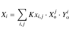
and
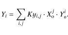
In these equations Xi and Yi correspond to the positions of the reference stars in the June 2006 reference frame, and
After transformation of the lists of point sources for each individual frame, the lists corresponding to a given observing epoch were combined. Average fluxes and positions as well as the corresponding uncertainties (the errors on the mean values) could be directly derived from the multiple measurements for each star. Sources that were not detected in multiple exposures were rejected as spurious detections.
Similar to Figs. A.2, A.3 shows the astrometric uncertainties of the sources detected in the 12 June 2004 epoch after (a) just applying shifts in x and y to combine the lists; and (b) after a full third order transformation into the reference frame. Again, it can be seen how the full polynomial transformation reduces the overall positional uncertainties and their systematic changes across the field considerably.
Appendix B: Offset field
B.1 Proper motions
The methodology applied to extract proper motions from the offset data set was identical to the one for the central field, except that no astrometric positions for the stars were derived. The analysis of the offset proper motions is based on three epochs only (August 2004, July 2005, and May 2008). Stars that were not detected in all three epochs were rejected from the sample. The stellar positions were just transferred roughly into the radio reference frame by applying appropriate offsets. We estimate that the uncertainties of the stellar positions in the offset field may reach up to several 0.1''. Therefore the proper motions for the offset field are not included in the list in Table B.1. The distances of the stars from Sgr A* were measured by using the NaCo pixel scale.
Table B.1: List of stars with measured proper motion in the GC.
The number stars with proper motions measured in the offset field, after applying the selection criteria, is 4308. In the left panel of Fig. B.1 we show a plot of reduced ![]() vs. Ks-band magnitude for the proper motion fits of the offset field
data. There is not such a clear correlation between
vs. Ks-band magnitude for the proper motion fits of the offset field
data. There is not such a clear correlation between
![]() and magnitude as in case of the center field data. We believe that this is mainly caused by (a) the low number statistics
of the offset field data (only 3 data points per fit) and (b) by the a factor
and magnitude as in case of the center field data. We believe that this is mainly caused by (a) the low number statistics
of the offset field data (only 3 data points per fit) and (b) by the a factor ![]() 2 (see Schödel et al. 2007) lower stellar surface number density in the offset field. The middle and right panels of Fig. B.1 show plots of the distribution of
2 (see Schödel et al. 2007) lower stellar surface number density in the offset field. The middle and right panels of Fig. B.1 show plots of the distribution of
![]() and velocity uncertainty for the offset field data.
and velocity uncertainty for the offset field data.
Figure B.2 shows an image of the offset field with measured stellar velocities indicated by arrows, after rejecting the stars with the 5% highest reduced ![]() -values in order to avoid outliers due to the small number of measured positions and thus rather
noisy statistics.
-values in order to avoid outliers due to the small number of measured positions and thus rather
noisy statistics.
| |
Figure B.1:
Error analysis for offset field data. Left: plot of log( |
| Open with DEXTER | |
![\begin{figure}
\par\includegraphics[width=17cm,clip]{0922figB2.eps}
\end{figure}](/articles/aa/full_html/2009/28/aa10922-08/img294.png) |
Figure B.2: Map of stars and measured proper motions of stars in the GC offset field. North is up and east is to the left. Arrows indicate magnitude and direction of the proper motion velocities. The black arrow in the lower left corner indicates the length of a 1000 km s-1 arrow. Please note that the map is not strictly astrometric. |
| Open with DEXTER | |
B.2 Velocity dispersion
We analysed the proper motion data for the offset field in the same way as the data for the central field. The mean projected radial and tangential velocities and the corresponding velocity dispersions are shown in Fig. B.3. The offset data set covers only a small angular section of the NSC and is highly incomplete at small R. Also, there are only three epochs available for the offset field. Therefore the quality of the offset data does not match the quality of the data on the central field. They have not been used for the further analysis in this work. The mean velocities show a larger scatter than in case of the center field data.
However, we believe that it is important to include the offset data in this work for two reasons. (a) They are centered on a different region of the cluster and can thus serve to detect systematic errors related to the alignment of the astrometric data with the reference epoch. We find that the proper motions for all stars common to the center and offset data agree within their ![]() uncertainties. (b) The offset data sample slightly larger distances from Sgr A*. They
support the image of a close to isotropic cluster with a constant velocity dispersion out to projected distances of R=30'' (1.14 pc).
uncertainties. (b) The offset data sample slightly larger distances from Sgr A*. They
support the image of a close to isotropic cluster with a constant velocity dispersion out to projected distances of R=30'' (1.14 pc).
![\begin{figure}
\par\includegraphics[width=15cm,clip]{0922figB3.eps}
\end{figure}](/articles/aa/full_html/2009/28/aa10922-08/img295.png) |
Figure B.3: Left: projected radial (green) and tangential (blue) velocity dispersions in the GC nuclear star cluster for the offset field (see Fig. 2). Right: mean projected radial and tangential velocities vs. projected distance from Sgr A* for the offset field. |
| Open with DEXTER | |
Footnotes
- ... mass
- Appendices are only available in electronic form at http://www.aanda.org
- ...
- Full Table B.1 is only available in electronic form at the CDS via anonymous ftp to cdsarc.u-strasbg.fr (130.79.128.5) or via http://cdsweb.u-strasbg.fr/cgi-bin/qcat?J/A+A/502/91
- ... telescope 4
- Based on observations collected at the European Southern Observatory, Chile, programs 071.B-0077, 073.B-0085, 073.B-0745, 073.B-0775, 075.B-0093, 075.C-0138, 077.B-0552, 081.B-0648
All Tables
Table 1: Details of the imaging observations used in this work.
Table 2: Measured proper motions, in the infrared frame, of the maser stars used for astrometric alignment.
Table B.1: List of stars with measured proper motion in the GC.
All Figures
| |
Figure 1: Mosaic image of the observations from 1 June 2006. A logarithmic gray scale has been adopted. The positions of IRS 7 and Sgr A* are indicated. North is up and east is to the left. Offsets in arcseconds from Sgr A* are indicated. Note that this mosaic image is only roughly astrometric. A constant pixel scale of 0.027'' per pixel has been assumed. Any residual net rotation of the image derotator has not been determined, i.e. the image may have a non-zero rotation angle (<1 deg). This may lead to offsets of up to a few tenths of arcseconds near the edge of the field. |
| Open with DEXTER | |
| In the text | |
| |
Figure 2: Mosaic image of the observations from 28 May 2008. The center of the image is offset about 20'' NE from Sgr A*. A logarithmic gray scale has been adopted. The positions of IRS 7, Sgr A*, and of the young and massive star IRS 8, that is surrounded by a bow-shock (Geballe et al. 2006), are indicated. North is up and east is to the left. Offsets in arcseconds from Sgr A* are indicated. Please note that this mosaic image is only roughly astrometric (see comments in caption of Fig. 1). |
| Open with DEXTER | |
| In the text | |
| |
Figure 3:
Error analysis for center field data. Top: plot of log(
|
| Open with DEXTER | |
| In the text | |
| |
Figure 4: Map of stars with measured proper motions in the GC central field. North is up and east is to the left. Arrows indicate magnitude and direction of the proper motion velocities. The black arrow in the lower left corner indicates the length of a 1000 km s-1 arrow. Positions and velocities of the stars are listed in in Table B.1. Early-type stars, identified by Paumard et al. (2006) and Buchholz et al. (2009) are indicated by red arrows. The small red circle marks the best candidate for a star escaping the cluster. |
| Open with DEXTER | |
| In the text | |
| |
Figure 5: Map of the systematic positional uncertainty of the astrometric positions of the stars listed in Table B.1. Contours are plotted in steps of 10 mas from 20 to 80 mas. |
| Open with DEXTER | |
| In the text | |
| |
Figure 6: Top: mean projected radial and tangential velocities vs. projected distance from Sgr A* ( left) and vs. angle east of north ( right). Mean values and the standard deviations annotated in the plots were calculated from the unweighted data points. Bottom: projected radial (green) and tangential (blue) velocity dispersions in the GC nuclear star cluster vs. projected distance from Sgr A* ( left) and vs. angle east of north ( right). These plots are based on the center data set (see Fig. 1) under the exclusion of identified early-type stars. |
| Open with DEXTER | |
| In the text | |
| |
Figure 7: Projected tangential proper motion of the maser stars vs. projected distance from Sgr A*. Black circles: radio proper motions; green boxes: infrared proper motions; red triangles: difference between radio and infrared proper motions. The straight line has been fitted to the difference data. No relative rotation between radio and infrared frames can be detected within the uncertainties of this analysis. |
| Open with DEXTER | |
| In the text | |
| |
Figure 8: Histograms of the direction angle, measured east of north, of measured stellar proper motions, for the distance bins 0''-5'', ''5''-10'', 10''-15'', and 15''-20''. To avoid confusion in the plot, the values in the 15''-20'' bin have been shifted by +40. |
| Open with DEXTER | |
| In the text | |
| |
Figure 9:
Left: map of the principal axes of the 2D velocity ellipses of the late-type stars on the plane of the sky. Right: histograms of the distribution of angles (measured north of east) defined by the longest axis of the velocity ellipses. The red histogram was calculated using only stars within |
| Open with DEXTER | |
| In the text | |
| |
Figure 10:
Left: histograms of the velocity parallel (green), |
| Open with DEXTER | |
| In the text | |
| |
Figure 11: LM mass estimator as a function of maximum projected distance from Sgr A*, based on the proper motions in the central field. Red: late-type stars; blue: early-type stars: black: combined sample. |
| Open with DEXTER | |
| In the text | |
| |
Figure 12:
Modelling the nuclear cluster assuming that all the mass is contained in the black hole and that the velocities are isotropic. The number density profile of the kinematical sample was assumed to be a single power law of the radius. Open circles are velocity dispersions computed using fixed radial bins; blue points are absolute values of the measured velocities. Straight lines show model predictions for
|
| Open with DEXTER | |
| In the text | |
| |
Figure 13:
Isotropic modelling of the nuclear cluster including a contribution to the gravitational potential from the stars, assumed to have a mass density that falls off
as
|
| Open with DEXTER | |
| In the text | |
| |
Figure 14:
Results of isotropic modelling of the NSC assuming the mass model of Eq. (14). The three parameters (
|
| Open with DEXTER | |
| In the text | |
| |
Figure 15:
|
| Open with DEXTER | |
| In the text | |
| |
Figure 16: Like Fig. 14, but for the anisotropic modelling. |
| Open with DEXTER | |
| In the text | |
| |
Figure 17: Like Fig. 15 but for the anisotropic modelling. |
| Open with DEXTER | |
| In the text | |
| |
Figure 18: Best-fit anisotropic model. a) and b) are the projected, radial and tangential velocity dispersions (black/solid lines), compared with a kernel-based velocity dispersion profile and associated (90%, 95%, 98%) confidence intervals (blue/dashed lines). c) Intrinsic velocity dispersions: radial (solid) and tangential (dashed) lines. |
| Open with DEXTER | |
| In the text | |
| |
Figure 19:
Anisotropic model with
|
| Open with DEXTER | |
| In the text | |
| |
Figure 20: Line-of-sight velocity vs. Galactic longitude. Blue circles: measurements from McGinn et al. (1989); green stars: measurements from Trippe et al. (2008). The straight orange line indicates the model of Trippe et al. (2008). The dashed black ellipses show the data that are not shown in Fig. 12 of Trippe et al. (2008). |
| Open with DEXTER | |
| In the text | |
| |
Figure 21:
Fits to the proper motion data when the BH mass is fixed to 4.0 |
| Open with DEXTER | |
| In the text | |
| |
Figure 22:
Enclosed stellar mass vs. distance from Sgr A*, derived from star counts and diffuse light density in the central parsec of the GC, using the broken-power law structure of the cluster from Schödel et al. (2007). The dashed lines indicate the statistical |
| Open with DEXTER | |
| In the text | |
| |
Figure A.1:
Transformation stars selected from the 1 June 2006 observations are marked by crosses on the FOV obtained after combining the dithered exposures. The average density of
transformation stars is indicated by the gray shading. Contour lines are drawn at
|
| Open with DEXTER | |
| In the text | |
| |
Figure A.2: Smooth maps of the positional uncertainty of the stars detected in the reference frame from 1 June 2006. After assigning the positional uncertainty of each star to its position, the map was smoothed by applying a Gaussian filter with a FWHM of 2.7''. The left panel shows the uncertainty of the stellar positions in the FOV after combining the astrometric lists from the individual exposures by applying just shifts in x and y coordinates (preliminary combined list, simple mosaicing). The right hand panel shows the uncertainties after aligning the stellar positions via a 3rd order polynomial fit (final combined list). Contour lines are drawn from 0 to 0.16 pixel at intervals of 0.02 pixel. The transformation reduces the overall uncertainty of the positions and eliminates systematic changes of the positional uncertainty due to camera distortions. The average combined uncertainty of all positions is 0.081 pixel before and 0.045 pixel after the polynomial fit. After applying a polynomial transformation to the stellar positions, the uncertainties correlate with the light density in the field. Light density variations arise from the combined effect of stellar density and the presence of bright stars. This can affect the astrometry via the photometric noise in the halos of the bright stars, especially since the used PSF was truncated (see Sect. 3). The unresolved stellar population will contribute as well to increased photometric noise. This can be seen when comparing the uncertainty map with the mosaic image shown in Fig. 1. One can, for example, see that the areas around IRS 7, IRS 1, or the IRS 16 cluster are clearly visible in the uncertainty map. The uncertainty of the stellar positions decreases with distance from Sgr A*, in correlation with the decreasing stellar density (see Schödel et al. 2007). |
| Open with DEXTER | |
| In the text | |
| |
Figure A.3: Smooth maps of the positional uncertainty of the stars detected in the reference frame from 12 June 2004. The maps were created in the same way as the maps shown in Fig. A.2. The left panel shows the uncertainty of the stellar positions in the FOV after combining the lists of detected stars by applying just shifts in x and y coordinates (simple mosaicing). The right hand panel shows the uncertainties after aligning the stellar positions with the reference frame via a polynomial fit. The transformation reduces the overall uncertainty of the positions and eliminates systematic changes of the positional uncertainty due to camera distortions. The average combined uncertainty of all positions is 0.073 pixel before and 0.027 pixel after the polynomial fit. The overall uncertainty is lower than for the stars in the reference frame because the quality of the AO correction was much better in the observing run on 12 June 2004. Therefore, the correlation of the uncertainty after the polynomial transform with the density of stars and the presence of bright stars is less obvious than in the 2006 data. However, areas of increased positional uncertainty are clearly associated with the IRS 7, IRS 16, and IRS 1. Please note that the different scaling of the maps in the left and right panels. The vertical strip of low uncertainties at the right edge of the FOV is an artifact due to the smoothing and the lack of sources in this area in the data from 12 June 2004. |
| Open with DEXTER | |
| In the text | |
| |
Figure B.1:
Error analysis for offset field data. Left: plot of log( |
| Open with DEXTER | |
| In the text | |
| |
Figure B.2: Map of stars and measured proper motions of stars in the GC offset field. North is up and east is to the left. Arrows indicate magnitude and direction of the proper motion velocities. The black arrow in the lower left corner indicates the length of a 1000 km s-1 arrow. Please note that the map is not strictly astrometric. |
| Open with DEXTER | |
| In the text | |
| |
Figure B.3: Left: projected radial (green) and tangential (blue) velocity dispersions in the GC nuclear star cluster for the offset field (see Fig. 2). Right: mean projected radial and tangential velocities vs. projected distance from Sgr A* for the offset field. |
| Open with DEXTER | |
| In the text | |
Copyright ESO 2009
Current usage metrics show cumulative count of Article Views (full-text article views including HTML views, PDF and ePub downloads, according to the available data) and Abstracts Views on Vision4Press platform.
Data correspond to usage on the plateform after 2015. The current usage metrics is available 48-96 hours after online publication and is updated daily on week days.
Initial download of the metrics may take a while.