| Issue |
A&A
Volume 501, Number 3, July III 2009
|
|
|---|---|---|
| Page(s) | 1113 - 1121 | |
| Section | The Sun | |
| DOI | https://doi.org/10.1051/0004-6361/200911800 | |
| Published online | 27 May 2009 | |
Magnetic field strength of active region filaments
C. Kuckein1 - R. Centeno2 - V. Martínez Pillet1 - R. Casini2 - R. Manso Sainz1 - T. Shimizu3
1 - Instituto de Astrofísica de Canarias, vía
Láctea s/n, 38205 La Laguna, Tenerife, Spain
2 - High Altitude Observatory (NCAR), Boulder, CO 80301, USA
3 - Institute of Space and Astronautical Science, JAXA, Sagamihara,
Kanagawa 229-8510, Japan
Received 5 February 2009 / Accepted 28 April 2009
Abstract
Aims. We study the vector magnetic field of a filament observed over a compact active region neutral line.
Methods. Spectropolarimetric data acquired with TIP-II (VTT, Tenerife, Spain) of the 10 830 Å spectral region provide full Stokes vectors that were analyzed using three different methods: magnetograph analysis, Milne-Eddington inversions, and PCA-based atomic polarization inversions.
Results. The inferred magnetic field strengths in the filament are around 600-700 G by all these three methods. Longitudinal fields are found in the range of 100-200 G whereas the transverse components become dominant, with fields as high as 500-600 G. We find strong transverse fields near the neutral line also at photospheric levels.
Conclusions. Our analysis indicates that strong (higher than 500 G, but below kG) transverse magnetic fields are present in active region filaments. This corresponds to the highest field strengths reliably measured in these structures. The profiles of the helium 10 830 Å lines observed in this active region filament are dominated by the Zeeman effect.
Key words: Sun: filaments - Sun: photosphere - Sun: chromosphere - Sun: magnetic fields - techniques: polarimetric
1 Introduction
The magnetic field strength of active region (AR) filaments has long remained poorly known or understood. The situation for quiescent filaments is notably more satisfactory since the early measurements back in the 70s (see, e.g., the review by López Ariste & Aulanier 2007). Field strengths measured in quiescent structures, mostly using the Hanle effect on the linear polarization of He I D3 at 5876 Å (e.g., Sahal-Brechot et al. 1977), were found to be in the range of 3-15 G (Leroy et al. 1983; see also the review by Anzer & Heinzel 2007). However, more recent measurements, which also took circular polarization into account, consistently show a tendency towards stronger field strengths. For example, the He I 10 830 Å investigation of Trujillo Bueno et al. (2002) and the He I D3 of Casini et al. (2003) found, respectively, field strengths of 20-40 G and 10-20 G (with field strengths up to 80 G in the latter set of observations). With similar techniques, using carefully inverted observations of the He I 10 830 Å lines, Merenda et al. (2006) find field strengths of about 30 G. Other recent works that also obtained relatively strong filament magnetic fields as compared with older measurements are Paletou et al. (2001) and Wiehr & Bianda (2003). Of particular interest are the high field strength areas revealed by Zeeman-dominated Stokes V profiles in conjunction with scattering dominated Q and U linear polarization signals obtained by Casini et al. (2003), showing how important it is to use all four Stokes parameters for a proper determination of the field strength in prominences.
Well-established properties of AR filaments are their systematically
stronger field strengths as compared to their quiescent counterparts, and
they lie lower in the atmosphere (see, e.g., Aulanier & Démoulin 2003).
Zeeman observations, using coronagraphs, provided field strengths for
AR prominences in the range of 50-200 G
(Tandberg-Hanssen & Malville 1974, and references therein).
However, the intrinsic difficulties of observing such low-lying structures
near the limb and the use of H![]() magnetography render these results somewhat
questionable (see López Ariste et al. 2005, for the problems associated with using a
Zeeman-based formulation of the measurements made in H
magnetography render these results somewhat
questionable (see López Ariste et al. 2005, for the problems associated with using a
Zeeman-based formulation of the measurements made in H![]() ).
Perhaps the most relevant modern estimate of the field strength in
AR prominences has been provided by Wiehr & Stellmacher (1991), who
measured the longitudinal magnetic field using the Stokes I and
V profiles of the Ca II IR triplet, finding a value of 150 G,
compatible with previous measurements.
It is important for the discussion presented in our paper
to note that, in that observational study, linear polarization
signals (Q and U) were not included. The only measurements of strong magnetic fields using an He I 10 830 Å full Stokes vector that we are aware of belong to a multicomponent flaring active region and reached values of
).
Perhaps the most relevant modern estimate of the field strength in
AR prominences has been provided by Wiehr & Stellmacher (1991), who
measured the longitudinal magnetic field using the Stokes I and
V profiles of the Ca II IR triplet, finding a value of 150 G,
compatible with previous measurements.
It is important for the discussion presented in our paper
to note that, in that observational study, linear polarization
signals (Q and U) were not included. The only measurements of strong magnetic fields using an He I 10 830 Å full Stokes vector that we are aware of belong to a multicomponent flaring active region and reached values of
![]() G (see Sasso et al. 2007).
G (see Sasso et al. 2007).
Because measurements are scarce, we are still far from having a
complete picture of the field strengths that permeate solar filaments.
Some progress has come from using photospheric distributions of (mostly
longitudinal) fields that are extrapolated into the corona (usually using models of
constant-![]() force-free field). The study by Aulanier & Démoulin (2003) is of
particular relevance to the present work. According to these authors, the
field strength of filaments found from the extrapolations is about 3 G
for the quiescent case, 40 G for active filaments (called ``plage
case'' in their work) and 15 G for intermediate cases.
The typical height in the atmosphere of a filament base ranges from 20 to 10 Mm, or
even lower, as one moves from quiescent to AR structures. These authors also
find positive field gradients with height that result in values of
0.1-1 G Mm-1, i.e., stronger fields are higher up in the atmosphere.
If these gradients are used to extrapolate down into the photosphere, the
fields there would be very similar to those found some Mm up in the
corona. For example a 10 Mm-height active filament with 100 G in the
corona would have no less than 90 G close to the photosphere. The
argument could also be turned around to start from the fields measured
near the photosphere, close to AR neutral lines (NLs), and
infer what the fields could be high in the corona. In the case of kG-strong
plage fields, with high density areal filling factors (that can
reach up to 50%; Martínez Pillet et al. 1997), one could expect fields
of several hundred Gauss within the filaments. Indeed,
Aulanier & Démoulin (1998, 2003) provide arguments supporting a
relationship between the photospheric fields at
the base of the filament and the filament fields up in the corona. They
conclude that the stronger the photospheric fields at the
base of the filament, the stronger the field in the filament itself.
Similarly, the separation of the two opposite polarity regions
scales inversely with the field strength of the filament, the latter being greater
whenever the two polarities are closer together. Dense (highly packed)
fields in the photosphere correspond indeed to
the photospheric configuration found below AR filaments as observed
recently by Lites (2005) and Okamoto et al. (2008). In both
cases, they find opposite polarity ``abutted'' plage fields at the
NL, with sheared horizontal fields in the hecto-Gauss range
and relatively high filling factors. These abutted field configurations seem to
also correspond with low-lying filaments structures. Lites (2005)
comments that the height of the filaments on top of the abutted plage
fields is no more than 2.5 Mm. Thus, high density (i.e., large
filling factor) horizontal plage fields near AR NLs, together with the
inferences from theoretical modeling (Aulanier & Démoulin 1998, 2003),
would indicate that fields of several hundred
Gauss can be expected in low-lying AR filaments.
force-free field). The study by Aulanier & Démoulin (2003) is of
particular relevance to the present work. According to these authors, the
field strength of filaments found from the extrapolations is about 3 G
for the quiescent case, 40 G for active filaments (called ``plage
case'' in their work) and 15 G for intermediate cases.
The typical height in the atmosphere of a filament base ranges from 20 to 10 Mm, or
even lower, as one moves from quiescent to AR structures. These authors also
find positive field gradients with height that result in values of
0.1-1 G Mm-1, i.e., stronger fields are higher up in the atmosphere.
If these gradients are used to extrapolate down into the photosphere, the
fields there would be very similar to those found some Mm up in the
corona. For example a 10 Mm-height active filament with 100 G in the
corona would have no less than 90 G close to the photosphere. The
argument could also be turned around to start from the fields measured
near the photosphere, close to AR neutral lines (NLs), and
infer what the fields could be high in the corona. In the case of kG-strong
plage fields, with high density areal filling factors (that can
reach up to 50%; Martínez Pillet et al. 1997), one could expect fields
of several hundred Gauss within the filaments. Indeed,
Aulanier & Démoulin (1998, 2003) provide arguments supporting a
relationship between the photospheric fields at
the base of the filament and the filament fields up in the corona. They
conclude that the stronger the photospheric fields at the
base of the filament, the stronger the field in the filament itself.
Similarly, the separation of the two opposite polarity regions
scales inversely with the field strength of the filament, the latter being greater
whenever the two polarities are closer together. Dense (highly packed)
fields in the photosphere correspond indeed to
the photospheric configuration found below AR filaments as observed
recently by Lites (2005) and Okamoto et al. (2008). In both
cases, they find opposite polarity ``abutted'' plage fields at the
NL, with sheared horizontal fields in the hecto-Gauss range
and relatively high filling factors. These abutted field configurations seem to
also correspond with low-lying filaments structures. Lites (2005)
comments that the height of the filaments on top of the abutted plage
fields is no more than 2.5 Mm. Thus, high density (i.e., large
filling factor) horizontal plage fields near AR NLs, together with the
inferences from theoretical modeling (Aulanier & Démoulin 1998, 2003),
would indicate that fields of several hundred
Gauss can be expected in low-lying AR filaments.
Given the observation that energetic coronal mass ejections (CMEs) are often associated with AR filament eruptions (see, e.g., Manchester et al. 2008; and Low 2001, for a review), it is highly desirable to develop diagnostic tools for direct measurements of the AR filament magnetic field and its evolution, from its emergence (see Okamoto et al. 2008) to the erupting phase. In this work, we present a clear diagnostic tool of how this can be achieved using full Stokes polarimetry of the He I 10 830 Å lines.
![\begin{figure}
\par {\hspace*{5mm}\includegraphics[width=6.9cm,clip]{11800f11.ps...
....ps}\hspace*{4.9mm}
\includegraphics[width=7.4cm,clip]{11800f16.ps}
\end{figure}](/articles/aa/full_html/2009/27/aa11800-09/img15.png) |
Figure 1: Top left: slit reconstructed continuum intensity map centered at the NL where the pores and penumbral-like formations can be identified. The location of the slit for the time series map is displayed. Top right: Si I Stokes V map normalized to the continuum intensity. Bottom: Stokes profiles observed at the slit position indicated in the top images and averaged over the time series (comprising 100 scans). The gray scale bar only applies to the polarization signals. The Zeeman-like signature of Stokes Q and Uare evident in this picture (He I lines are centered at 0 and 1.2 Å approximately. The zero in the wavelength scale corresponds to 10 829.09 Å). The arrows indicate the position of the presented Stokes profiles in Figs. 3 and 4. |
| Open with DEXTER | |
2 Observations
The observations described in this paper were carried out at the German Vacuum
Tower Telescope (VTT, Tenerife, Spain) on the 3rd and the 5th of July, 2005, using
the Tenerife Infrared Polarimeter (TIP-II, Collados et al. 2007). TIP-II allows to measure
the full Stokes vector (almost) simultaneously for all the pixels along the
spectrograph slit. The slit (0
![]() 5 wide and 35
5 wide and 35
![]() long) was placed over
the target, a filament lying over the NL of active region NOAA 10781 situated
close to disk center (at coordinates N13-W4 around
long) was placed over
the target, a filament lying over the NL of active region NOAA 10781 situated
close to disk center (at coordinates N13-W4 around ![]() on July 3rd and
at N13-W29 or
on July 3rd and
at N13-W29 or ![]() on July 5th) with the help of context H
on July 5th) with the help of context H![]() and
continuum images. The H
and
continuum images. The H![]() frames showed the filament lying always on top
of bright plage regions visible immediately to either side of the absorption feature.
It is likely that the results presented in this paper particularly apply to
such an ``active'' filament configuration. SOHO/MDI (Scherrer et al. 1995)
magnetograms and continuum frames have been used to follow the evolution of the
active region as it crossed the visible surface. The active region was
identified to be in its slow decay mode, encompassing a round symmetric leader
sunspot and a follower, spotless, plage region. At the location of the NL,
sporadic pore-like formations and penumbral-like configurations (with no evident
radially symmetric link to an umbral or pore structure as normal penumbra or partial
penumbrae do) were seen, especially on the 5th of July data-sets. Pores near the NL with both polarities
are identified and the penumbral-like region seems to correspond to field lines connecting
them. The NL was oriented in the N-E direction and showed a very compact
configuration, with the two polarities always remaining in close contact. The
leader sunspot became invisible on the 6th of July after decreasing in size
while approaching the west solar limb.
frames showed the filament lying always on top
of bright plage regions visible immediately to either side of the absorption feature.
It is likely that the results presented in this paper particularly apply to
such an ``active'' filament configuration. SOHO/MDI (Scherrer et al. 1995)
magnetograms and continuum frames have been used to follow the evolution of the
active region as it crossed the visible surface. The active region was
identified to be in its slow decay mode, encompassing a round symmetric leader
sunspot and a follower, spotless, plage region. At the location of the NL,
sporadic pore-like formations and penumbral-like configurations (with no evident
radially symmetric link to an umbral or pore structure as normal penumbra or partial
penumbrae do) were seen, especially on the 5th of July data-sets. Pores near the NL with both polarities
are identified and the penumbral-like region seems to correspond to field lines connecting
them. The NL was oriented in the N-E direction and showed a very compact
configuration, with the two polarities always remaining in close contact. The
leader sunspot became invisible on the 6th of July after decreasing in size
while approaching the west solar limb.
Two observing strategies were used to map the NL region. Several spatial scans
that covered the whole AR were carried out in the course of the 3 days, and one
time series (with the slit fixed over the filament) was taken on July 5th. This
data-set was averaged in time in order to improve the signal-to-noise (S/N)
ratio of the spectral profiles. The pixel size along the slit was
0
![]() 17 and the scanning step (in the case of the rasters) was 0
17 and the scanning step (in the case of the rasters) was 0
![]() 3
per step. The
exposure time per slit position was 8 seconds. The adaptive optics system
(KAOS, von der Lühe et al. 2003) was locked on nearby pores during all the runs,
substantially improving the image quality of the observations carried out during
relatively poor seeing conditions, and providing a final estimated spatial
resolution of
3
per step. The
exposure time per slit position was 8 seconds. The adaptive optics system
(KAOS, von der Lühe et al. 2003) was locked on nearby pores during all the runs,
substantially improving the image quality of the observations carried out during
relatively poor seeing conditions, and providing a final estimated spatial
resolution of ![]() 1
1
![]() .
Flat-field and dark current corrections were
performed for all the data-sets and, in order to compensate for the telescope
instrumental polarization, we also carried out the standard polarimetric
calibration (Collados 1999; Collados 2003) for this instrument.
.
Flat-field and dark current corrections were
performed for all the data-sets and, in order to compensate for the telescope
instrumental polarization, we also carried out the standard polarimetric
calibration (Collados 1999; Collados 2003) for this instrument.
The observed spectral range spanned from 10 825 to 10 836 Å, with a spectral
sampling of ![]() 11.1 mÅ px-1. However, a 3px binning in the spectral
domain was applied to all the data to increase the S/N while still preserving
subcritical sampling. The 10 830 Å spectral region is a powerful diagnostic
window of the solar atmospheric properties since it contains valuable
information coming simultaneously from the photosphere (carried by the
Si I line at 10 827 Å) and the chromosphere (encoded in the He I 10 830 Å triplet). This He multiplet originates between a lower term 23S1 and
an upper term 23P2,1,0. Thus, it comprised three spectral lines,
namely a ``blue'' component at 10 829.09 Å (
11.1 mÅ px-1. However, a 3px binning in the spectral
domain was applied to all the data to increase the S/N while still preserving
subcritical sampling. The 10 830 Å spectral region is a powerful diagnostic
window of the solar atmospheric properties since it contains valuable
information coming simultaneously from the photosphere (carried by the
Si I line at 10 827 Å) and the chromosphere (encoded in the He I 10 830 Å triplet). This He multiplet originates between a lower term 23S1 and
an upper term 23P2,1,0. Thus, it comprised three spectral lines,
namely a ``blue'' component at 10 829.09 Å (
![]() )
and a
``red'' component at
)
and a
``red'' component at
![]() Å that results from the remaining two
transitions (
Å that results from the remaining two
transitions (
![]() ), which appear completely blended at
typical solar atmospheric temperatures.
This multiplet is formed in the high chromosphere (Avrett et al. 1994) with no
contribution from photospheric levels, and serves as a unique diagnostic tool for
chromospheric magnetic fields. In filament structures, the height of formation of this
multiplet corresponds to the height of the opaque material inside them, which might
well correspond to typical coronal heights.
), which appear completely blended at
typical solar atmospheric temperatures.
This multiplet is formed in the high chromosphere (Avrett et al. 1994) with no
contribution from photospheric levels, and serves as a unique diagnostic tool for
chromospheric magnetic fields. In filament structures, the height of formation of this
multiplet corresponds to the height of the opaque material inside them, which might
well correspond to typical coronal heights.
2.1 Predominance of Zeeman-like signatures in AR filament He I 10 830 Å Stokes profiles
The most striking finding encountered during the analysis of the data from this campaign was the ubiquitous presence of Zeeman-like signatures in the Stokes Q and U profiles of the He I lines in the AR filament (see Fig. 1). Recent observations of this triplet carried out with the same instrument (Trujillo Bueno et al. 2002) have shown quiescent filament Stokes profiles dominated by atomic level polarization (and its modification through the Hanle effect). These forward-scattering signatures (see Fig. 4 of Trujillo Bueno et al. 2002) correspond to one-lobe profiles that are positive for the red component of the He triplet and negative for the blue one (in the positive Stokes Qreference system) due, respectively, to selective emission and absorption processes induced by the anisotropic illumination of the He atoms. However, in the present case, the Stokes Q and U signals of the blue and red components of the multiplet, exhibit the usual three-lobe profile that is expected from the Zeeman effect (right panel of Fig. 1). While some influence of atomic polarization in these profiles cannot be ruled out a priory, it is clear that an explanation of their shapes should rely mainly on the Zeeman and Paschen-Back effects. This fact, interesting in itself, will be briefly discussed below (Sect. 3.3).
The continuum frame in the top panel of Fig. 1 was
reconstructed from the various slit scan positions (thus reflecting the real spatial
resolution of the data) of a map centered at the NL. This data-set was taken on the 5th of
July, 2005. The presence of pores and penumbral-like structures
is evident in this frame and their location corresponds to the NL. Right after this map,
a time series with the slit fixed over the NL
was performed in order to produce high S/N Stokes profiles.
The bottom four panels of Fig. 1 correspond to the
Stokes parameters obtained after averaging over the full time series
(100 scans), which resulted
in a S/N of about 4000. The inversions performed later in this work were
carried
out on the spectral profiles extracted from this time-averaged data-set. The location of the NL
had to be guessed in real-time during the observations. The chosen slit position for the
time series is represented
by a vertical black line in the continuum frame of Fig. 1.
Posterior analysis has
shown that this location was a few arcsec off at one side of the actual NL, and that the
slit would have been more correctly placed at x=18
![]() (referred to the abscissa coordinates in the continuum panel)
instead of at x=20
(referred to the abscissa coordinates in the continuum panel)
instead of at x=20
![]() .
Nevertheless, indications of polarity changes along the slit
in the Si I line (evident around y=13
.
Nevertheless, indications of polarity changes along the slit
in the Si I line (evident around y=13
![]() in the Stokes V
map of the same
figure) show that we were not very far away from it.
in the Stokes V
map of the same
figure) show that we were not very far away from it.
Inspection of the profiles at other slit locations, and of similar maps taken on the 3rd of July, consistently exhibited Zeeman-dominated linear polarization signals in those regions where the He line showed strong absorption features. However, in regions with weak He absorption (typically near the boundaries of the filament), we often find linear profiles dominated by scattering polarization signatures, similar to those observed by Trujillo Bueno et al. (2002). This indicates that, in general, the profiles obtained in AR filaments can have significant contributions from various competing physical processes: the atomic level polarization due to the anisotropic illumination of the He atoms, the modification of these population imbalances induced by the presence of a magnetic field inclined with respect to the axis of symmetry (Hanle effect), and the Zeeman splitting characteristic of strong magnetic fields. A detailed study with these physical ingredients for all the maps observed at this NL is beyond the scope of this paper. In the present work, we concentrate on the implications of the clear Zeeman-dominated signatures observed almost everywhere in this filament.
One point is worth mentioning after a simple visual inspection of
Fig. 1. A comparison of the signs displayed by the
linear polarization profiles of the He I and Si I lines shows that
the orientation of the vector magnetic field is different in the filament than
in the underlying photosphere. In the Stokes Q frame, the He I 3-lobed
profiles have the same sign all along the slit whereas the Si I line (and all the other smaller photospheric features at redder wavelengths)
exhibits a change in sign around y=23
![]() .
Conversely, in the Stokes U frame, the
photospheric signals have a 3-lobed sign distribution that remains constant
almost all along the spatial domain while the He I lines now show a sign reversal
near the middle of the slit. An analysis based on the formula for the azimuth angle by Auer et al. (1977) gives an estimate of this difference between the azimuths inferred from the Si I and He I lines. Around y = 5
.
Conversely, in the Stokes U frame, the
photospheric signals have a 3-lobed sign distribution that remains constant
almost all along the spatial domain while the He I lines now show a sign reversal
near the middle of the slit. An analysis based on the formula for the azimuth angle by Auer et al. (1977) gives an estimate of this difference between the azimuths inferred from the Si I and He I lines. Around y = 5
![]() we obtain values of the azimuth which differ in
we obtain values of the azimuth which differ in
![]() .
This readily shows that the 10 830 Å spectral region has a great potential to diagnose the orientation of the magnetic field
from the photosphere all the way up to the filament. We postpone this study to a future paper.
.
This readily shows that the 10 830 Å spectral region has a great potential to diagnose the orientation of the magnetic field
from the photosphere all the way up to the filament. We postpone this study to a future paper.
3 Vector magnetic field near the AR neutral line
Several analyses with various levels of complexity have been performed on the reduced data. The first approach was a simple magnetograph-like analysis based on the assumption of the weak-field approximation as formulated below. This method was applied to all the points in one of the maps obtained during the campaign. We subsequently performed an analysis of the high S/N spectral profiles obtained from the averaged time series with a Milne-Eddington (ME) code and later with a more sophisticated inversion procedure based on principal component analysis (PCA) of a statistically generated database of spectral profiles that account for the physics of atomic level polarization and the Hanle effect. All these different methods consistently yield transverse field strengths in the filament well above 500 G.
3.1 Magnetograph analysis
Typical Doppler widths for the red He I line are in the range of 200-300 mÅ. The Landé
factors are 1.75 and 1.25 for the
![]() and the
and the
![]() transitions, respectively. If the transitions are weighted with their line strengths,
an average Landé factor of
transitions, respectively. If the transitions are weighted with their line strengths,
an average Landé factor of
![]() 1.42 for the red component of the helium multiplet
is obtained. This Landé factor translates the above
Doppler widths to field strengths in the range of 2000-3000 G,
which is much stronger than the fields we expect for AR filaments. Together with the
assumption that the observed
signals are due to the Zeeman effect, these large Doppler widths justify the use of the
well-known weak field approximation (see, e.g., Landi Degl'Innocenti 1992) as a first approach to
infer the magnetic field from the data.
In this approximation, the relation between the longitudinal field strength and Stokes
V profile is given by:
1.42 for the red component of the helium multiplet
is obtained. This Landé factor translates the above
Doppler widths to field strengths in the range of 2000-3000 G,
which is much stronger than the fields we expect for AR filaments. Together with the
assumption that the observed
signals are due to the Zeeman effect, these large Doppler widths justify the use of the
well-known weak field approximation (see, e.g., Landi Degl'Innocenti 1992) as a first approach to
infer the magnetic field from the data.
In this approximation, the relation between the longitudinal field strength and Stokes
V profile is given by:
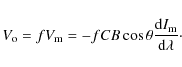
The subscript ``o'' stands for the observed profile, while ``m'' represents the profile generated in the magnetic component that fills a fraction f of the resolution element; B is the field strength,
| (2) |
with the subscript ``nm'' referring to the non-magnetic component. The last factor in the right-hand-side of Eq. (1) is the derivative of
The
![\begin{figure}
\par\includegraphics[width=5.6cm,clip]{11800f21.ps}\hspace*{2.8mm...
...25.ps}\hspace*{2.5mm}
\includegraphics[width=6cm,clip]{11800f26.ps}
\end{figure}](/articles/aa/full_html/2009/27/aa11800-09/img39.png) |
Figure 2: From left to right and top to bottom: He I Doppler width, Si I LOS magnetic field, He I LOS magnetic field, He I core intensity, Si I transverse magnetic field and He I transverse magnetic field. The corresponding continuum intensity frame can be seen in the top panel of Fig. 1. |
| Open with DEXTER | |
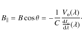
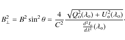
For transverse fields, a similar equation applies including
the quadratic dependence of the linear polarization signals on
the transverse component of the field
and the second derivative of the Stokes I profile with respect to ![]() .
A similar argument gives:
.
A similar argument gives:
Like in the equation for the longitudinal field, the filling factor (of a non-magnetic component) is absent. On the other hand, and in contrast to Eq. (3), the right hand side of Eq. (4) must be computed at the central wavelength,
Thus, and in order to obtain high S/N maps of the chromospheric
transverse fields, we averaged the unsigned Q and U signals over
three wavelengths, the central wavelength and two wavelengths at 278 mÅ
on each side of line center, corresponding approximately to the locations of the peak
signals in the linear polarization profiles, so
where
A similar approach was followed with the Si I line to obtain the
photospheric magnetic field. The Landé factor for this line is 1.5.
The spectral profiles arising from this transition are broad enough to partly justify
the application of the weak-field approximation. However, like for any other photospheric line,
the vector-magnetograph data obtained with this method have to be interpreted with caution.
In particular, the results for this line are affected by filling factor effects as is the
case for commonly used photospheric
magnetograph data. For the Si I line, the exact formulation of Eq. (4) was
used. The intrinsically greater photospheric magnetic field strengths together with the
fact that the Si I Stokes I profile has a sizeable second derivative, makes
the determination of ![]() less affected by noise when using only the central wavelength
point of the linear polarization profiles for its determination.
less affected by noise when using only the central wavelength
point of the linear polarization profiles for its determination.
Lastly, the Stokes I profiles of both He I and Si I were fitted with Gaussian functions from which the line center, line width and strength were inferred. In the case of the He I, this approach proved very useful to identify the location of the filament above the NL.
The results from this approach are presented in Fig. 2 for
the map observed on the 5th of July. The He I Doppler width and line core
frames show that the line becomes deeper and narrower inside the filament. This
could be an indication of the presence of a denser and cooler plasma than in
its immediate plage surroundings. These frames also reveal that the filament
has a highly twisted topology, with filamentary threads running at almost 45 degrees from the direction defined by the NL. This becomes evident when
compared to the Si and He LOS magnetograms. The twist in the filament is more
obvious in the bottom half of the frames than in the top part, where a more
diffuse linear topology is observed. These twisted signatures could be clearly
seen in the observations from the 5th of July, while they were hardly visible
in the maps obtained two days earlier. The Si I LOS magnetogram
shows that the separation between the two polarities is less than 5
![]() at
photospheric levels when the magnetogram is scaled at
at
photospheric levels when the magnetogram is scaled at ![]() 1000 G. A tighter
scaling with a smaller threshold would provide a much narrower NL channel. In
the He I LOS magnetograms, with a scaling of
1000 G. A tighter
scaling with a smaller threshold would provide a much narrower NL channel. In
the He I LOS magnetograms, with a scaling of ![]() 400 G, the
channel is practically absent, showing how intense the plage surrounding this
AR filament was. A thread-like structure in the longitudinal component running
parallel to the direction of the twist (i.e. at 45 degrees from the NL) in the
mid range of the frame is observed. Note that the AR is 22 degrees off disk
center so horizontal threads in the filament can give rise to sizeable Stokes
V signals. The intrinsic LOS magnetic field strength at the NL (we stress
that no filling factor effect is included in these estimates) is typically 100 G for each of the two polarities (in agreement with older measurements of AR
filaments that did not include transverse field measurements). The neighboring
plage displays an intrinsic longitudinal field strength of 200-400 G. If we
assume an intrinsic photospheric field strength in the plage of 1400 G (see
Martínez Pillet et al. 1997), this would indicate a filling factor of about 20% in
this layer.
400 G, the
channel is practically absent, showing how intense the plage surrounding this
AR filament was. A thread-like structure in the longitudinal component running
parallel to the direction of the twist (i.e. at 45 degrees from the NL) in the
mid range of the frame is observed. Note that the AR is 22 degrees off disk
center so horizontal threads in the filament can give rise to sizeable Stokes
V signals. The intrinsic LOS magnetic field strength at the NL (we stress
that no filling factor effect is included in these estimates) is typically 100 G for each of the two polarities (in agreement with older measurements of AR
filaments that did not include transverse field measurements). The neighboring
plage displays an intrinsic longitudinal field strength of 200-400 G. If we
assume an intrinsic photospheric field strength in the plage of 1400 G (see
Martínez Pillet et al. 1997), this would indicate a filling factor of about 20% in
this layer.
In both, the photospheric and chromospheric magnetograms, the region where the
longitudinal field becomes weaker corresponds to the region with very strong
transverse fields. The somewhat wider photospheric NL channel corresponds to a
wider photospheric area occupied with strong transverse fields, while the
transverse fields in the chromosphere fill a narrower region. These transverse
fields seem to follow the structures observed in the He line core frame: a more
linear topology in the top part and a twisted formation in the bottom half.
What becomes readily surprising is the magnitude of the transverse fields
observed in the chromosphere (and to the extent that the weak field
approximation is valid, in the photosphere as well). The photosphere shows
fields in the range of up to kG in the region between abscissae x=15
![]() to x=20
to x=20
![]() in the frames of Fig. 2. This area shows
penumbral-like structures and pores in the white light image. It is clear
that these orphan penumbral-like regions are magnetically linked to the main body of
the AR filament and correspond to horizontal field lines at the photospheric
surface. The transverse fields derived from the Si I line
undoubtedly show the twist configuration similar to that observed in the
He I lines. In the chromosphere, the transverse fields are also
strong. The present analysis yields transverse fields with strengths in the
range of 500-600 G, strongly concentrated in the narrow NL channel. Note that
this region, at best, a few arcsec wide, is below the low resolutions
of old observations. These high transverse magnetic fields are well above
most, if not all, of past field strength measurements in AR filaments.
in the frames of Fig. 2. This area shows
penumbral-like structures and pores in the white light image. It is clear
that these orphan penumbral-like regions are magnetically linked to the main body of
the AR filament and correspond to horizontal field lines at the photospheric
surface. The transverse fields derived from the Si I line
undoubtedly show the twist configuration similar to that observed in the
He I lines. In the chromosphere, the transverse fields are also
strong. The present analysis yields transverse fields with strengths in the
range of 500-600 G, strongly concentrated in the narrow NL channel. Note that
this region, at best, a few arcsec wide, is below the low resolutions
of old observations. These high transverse magnetic fields are well above
most, if not all, of past field strength measurements in AR filaments.
The various maps for the observations on the 3rd of July support the hypothesis
that an AR filament corresponds to a narrow channel characterized with strong
(![]() G) transverse fields. There is a clear spatial correlation between
strong absorption signatures in He I (measured by the line core
intensities), and narrow (or ``abutted'') plage regions with strong transverse
fields in the chromosphere. A complete description of all these maps is
postponed to a future paper. But it is interesting to point out the
following main differences with the map of Fig. 2: the absence
of evident twisted threads, the absence of penumbral-like regions in
white-light maps, weaker and more diffuse transverse fields at the photosphere
(not reaching kG levels) and the presence of weaker He I
absorption signatures in regions outside the intense NL channel that display
atomic polarization signals.
G) transverse fields. There is a clear spatial correlation between
strong absorption signatures in He I (measured by the line core
intensities), and narrow (or ``abutted'') plage regions with strong transverse
fields in the chromosphere. A complete description of all these maps is
postponed to a future paper. But it is interesting to point out the
following main differences with the map of Fig. 2: the absence
of evident twisted threads, the absence of penumbral-like regions in
white-light maps, weaker and more diffuse transverse fields at the photosphere
(not reaching kG levels) and the presence of weaker He I
absorption signatures in regions outside the intense NL channel that display
atomic polarization signals.
![\begin{figure}
\par\includegraphics[width=12.2cm,clip]{11800fg3.ps}
\end{figure}](/articles/aa/full_html/2009/27/aa11800-09/img48.png) |
Figure 3:
Stokes profiles of the He I 10 830 Å triplet at a height
of 8 arcsec in Fig. 1
in the mid portion of the twisted region of the
filament. The dots represent the observed profiles obtained after averaging
the time series in order to achieve a higher S/N. The solid line corresponds
to the best fit achieved with a Milne-Eddington inversion code that takes
into account the IPB effect. The magnetic field obtained from
this particular fit is
|
| Open with DEXTER | |
3.2 Milne-Eddington inversions
The interest of the magnetograph analysis is that it is easily
computed over a complete map with a very low computational effort. However, in
order to validate the weak-field approximation inferences of the magnetic
field strength in the filament, we carried out a Milne-Eddington (ME) inversion
of the He I Stokes profiles of the averaged time series. These
high S/N data correspond to the location of the vertical line at x=20
![]() in the map of Fig. 1. The inversion code we used
(MELANIE; Socas-Navarro 2001) computes the Zeeman-induced Stokes spectra - in the
incomplete Paschen-Back (IPB) effect regime - that emerge from a model
atmosphere described by the Milne-Eddington approximation. This assumes a
semi-infinite constant-property atmosphere whose source function varies
linearly with optical depth,
in the map of Fig. 1. The inversion code we used
(MELANIE; Socas-Navarro 2001) computes the Zeeman-induced Stokes spectra - in the
incomplete Paschen-Back (IPB) effect regime - that emerge from a model
atmosphere described by the Milne-Eddington approximation. This assumes a
semi-infinite constant-property atmosphere whose source function varies
linearly with optical depth, ![]() .
This approach does not account for the
atomic-level polarization induced by the anisotropic radiation pumping of the
He atoms from the underlying photospheric continuum.
.
This approach does not account for the
atomic-level polarization induced by the anisotropic radiation pumping of the
He atoms from the underlying photospheric continuum.
For magnetic fields between 400 and 1500 G the Zeeman splitting of the upper J-levels of the He I triplet is comparable to their energy separation. Thus, it is crucial to compute the energy levels in the IPB regime to avoid an under-estimation of the magnetic field strength when carrying out the inversion to interpret observations (Socas-Navarro et al. 2004; Sasso et al. 2006).
The Milne-Eddington model atmosphere uses a set of eleven free parameters that
the inversion code modifies in an iterative manner in order to obtain the best fits to
the observed Stokes profiles. These free parameters are: the magnetic field strength (B),
its inclination (![]() )
and azimuth (
)
and azimuth (![]() )
angles in the
reference system of the observer (the azimuth is measured
with respect to the local solar radial direction), the line strength (
)
angles in the
reference system of the observer (the azimuth is measured
with respect to the local solar radial direction), the line strength (![]() ),
the Doppler width (
),
the Doppler width (
![]() ), a damping parameter, the LOS velocity, the source
function at
), a damping parameter, the LOS velocity, the source
function at ![]() and its gradient, a macroturbulence factor and a stray light
fraction f.
An initial guess model must be provided to the code. In order to prevent the inversion scheme
from getting locked into local minima, we carried out the inversions using several different
initializations, in which B,
and its gradient, a macroturbulence factor and a stray light
fraction f.
An initial guess model must be provided to the code. In order to prevent the inversion scheme
from getting locked into local minima, we carried out the inversions using several different
initializations, in which B, ![]() and
and ![]() were taken from
the above-described magnetograph analysis and the remaining parameters were obtained
from random perturbations of reasonable pre-set values.
All parameters were free except for the stray light fraction, which was set to zero
(i.e., assuming a filling factor of 1; we refer to the explanation in Sect 3.1).
We stress that, even if the data is contaminated with stray-light from the surroundings,
using a filling factor of unity allows a direct comparison with the results
given in the previous section.
were taken from
the above-described magnetograph analysis and the remaining parameters were obtained
from random perturbations of reasonable pre-set values.
All parameters were free except for the stray light fraction, which was set to zero
(i.e., assuming a filling factor of 1; we refer to the explanation in Sect 3.1).
We stress that, even if the data is contaminated with stray-light from the surroundings,
using a filling factor of unity allows a direct comparison with the results
given in the previous section.
Figures 3 and 4
show the results of the ME inversion of the full Stokes
vector for two positions along the filament (only two
fits are shown but the complete set of profiles from
Fig. 1
were inverted). The excellent performance of the ME inversion
tells us that there are barely any scattering polarization signatures in these
profiles, and that the formation physics of the multiplet is adequately described
in the IPB regime. As expected, the magnetic field strengths inferred from all the
inversions are around 600-700 G with very high
inclinations (
![]() )
with respect to the line-of-sight, thus confirming the existence of
strong transverse
fields in this AR filament. The exact values obtained for
Fig. 3
are
)
with respect to the line-of-sight, thus confirming the existence of
strong transverse
fields in this AR filament. The exact values obtained for
Fig. 3
are
![]() G and
G and
![]() G while for
Fig. 4 we
obtain
G while for
Fig. 4 we
obtain
![]() G and
G and
![]() G.
In the solar reference frame, the magnetic field
vector turns out to be close to horizontal, 59
G.
In the solar reference frame, the magnetic field
vector turns out to be close to horizontal, 59![]() and 99
and 99![]() of
inclination with respect to the local vertical, respectively.
of
inclination with respect to the local vertical, respectively.
The magnetic field strengths derived from the weak field
regime analysis are systematically under-estimated by
![]() G, but
the retrieved inclinations and azimuths are in very good agreement with those
obtained from the ME-IPB inversions. This means that the weak field approximation
yields a reliable magnetic field topology and a low-end value for the field strength.
G, but
the retrieved inclinations and azimuths are in very good agreement with those
obtained from the ME-IPB inversions. This means that the weak field approximation
yields a reliable magnetic field topology and a low-end value for the field strength.
3.3 PCA-based atomic polarization inversion
The observations described above were also independently inverted using the principal component analysis (PCA) approach described by López Ariste & Casini (2002). In fact, pattern recognition techniques are particularly well suited to attack ill-defined inversion problems characterized by computationally intensive forward problems. This is exactly the case for spectropolarimetric inversions in prominences and filaments, where the Stokes profiles are often formed by the scattering of resonant radiation. The computation of the emergent polarization in such case requires the preliminary solution of the non-LTE problem of atomic-level excitation by anisotropic illumination of the plasma from the underlying photosphere. The presence of a magnetic field further modifies the ensuing atomic polarization through the Hanle effect (see, e.g. Landi Degl'Innocenti & Landolfi 2004, for a review of atomic polarization effects). This problem, which is totally by-passed in the ME approach to spectropolarimetric inversion, completely dominates the numerical computation of line polarization in radiation scattering. For this reason, pattern recognition techniques provide a very attractive strategy to Stokes inversion for radiation scattering, since the numerically intensive forward problem is solved once and for all for a comprehensive set of illumination, thermodynamic, and magnetic conditions in the plasma for the problem at hand. The goal of these techniques is thus to build universal databases of profiles that can be searched for the solution to any given Stokes inversion problem. Principal component analysis additionally provides a way of compressing database information, by reducing it to a few principal component profiles that contain all the fundamental physics of the formation of the emergent Stokes profiles (López Ariste & Casini 2002; Casini et al. 2005).
![\begin{figure}
\par\includegraphics[width=13cm,clip]{11800fg4.ps}
\end{figure}](/articles/aa/full_html/2009/27/aa11800-09/img61.png) |
Figure 4:
Same as Fig. 3
but for a profile near the bottom portion of the
twisted region of the filament (at a height of 5 arcsec).
The fitted parameters for the ME case are
|
| Open with DEXTER | |
For the inversion of the observations illustrated in this paper, we created a
database of 250 000 profiles, spanning all possible orientations of the
magnetic field, with strengths between 0 and 2000 G. The illumination
conditions were set by the radiation temperature and center-to-limb variation
(CLV) profile of the photospheric radiation at 1 ![]() m (Cox 2000), and by
assuming a range of scattering heights between 0 and 0.06
m (Cox 2000), and by
assuming a range of scattering heights between 0 and 0.06 ![]() (42 Mm).
The LOS inclination in the database used for the inversion of the July 5, 2005,
observations spanned between 20
(42 Mm).
The LOS inclination in the database used for the inversion of the July 5, 2005,
observations spanned between 20![]() and 30
and 30![]() .
The thermal Doppler
width and micro-turbulent velocity, responsible for the overall profile
broadening, were accounted for by introducing an equivalent temperature
spanning between 104 and
.
The thermal Doppler
width and micro-turbulent velocity, responsible for the overall profile
broadening, were accounted for by introducing an equivalent temperature
spanning between 104 and
![]() K. Finally, the database Stokes
profiles were calculated by integrating the polarized radiation emerging from a
homogeneous slab with optical depth at line center varying between 0.2 and 1.4.
Very soon it was realized that such conventional scattering scenario could not
fit satisfactorily the observations, unless some additional depolarizing
mechanism could be accounted for to explain the surprisingly low level of
atomic polarization revealed by the Zeeman-like shape of the Stokes Q and Uprofiles. For this reason, in the creation of the inversion database we
introduced an ad-hoc weight factor for the anisotropy of the photosphere
radiation, ranging between 0 and 1. Extensive inversion tests that were run
over the entire filament map consistently gave anisotropy weight factors
significantly smaller than unity, with a predominance of values around 0.2,
thus confirming the presence of some unidentified depolarizing mechanism in the
formation of the observed profiles. The possible physical origin of such
depolarization has been extensively discussed by Casini et al. (2009), but see also
Trujillo Bueno & Asensio Ramos (2007).
K. Finally, the database Stokes
profiles were calculated by integrating the polarized radiation emerging from a
homogeneous slab with optical depth at line center varying between 0.2 and 1.4.
Very soon it was realized that such conventional scattering scenario could not
fit satisfactorily the observations, unless some additional depolarizing
mechanism could be accounted for to explain the surprisingly low level of
atomic polarization revealed by the Zeeman-like shape of the Stokes Q and Uprofiles. For this reason, in the creation of the inversion database we
introduced an ad-hoc weight factor for the anisotropy of the photosphere
radiation, ranging between 0 and 1. Extensive inversion tests that were run
over the entire filament map consistently gave anisotropy weight factors
significantly smaller than unity, with a predominance of values around 0.2,
thus confirming the presence of some unidentified depolarizing mechanism in the
formation of the observed profiles. The possible physical origin of such
depolarization has been extensively discussed by Casini et al. (2009), but see also
Trujillo Bueno & Asensio Ramos (2007).
The results of the PCA inversion are overplotted to the ME inversions as dot-dashed lines in
Figs. 3 and 4. The PCA inversion provides a magnetic field of B=667 G in the first case and B = 664 G in the second. The inclination angles are almost the same as the ones obtained by the ME inversions,
![]() and
and
![]() with respect to the local vertical, respectively. The inferred magnetic field azimuths are also in very good agreement.
with respect to the local vertical, respectively. The inferred magnetic field azimuths are also in very good agreement.
4 Conclusions
The He I 10 830 Å lines observed in a filament at the NL of active region
NOAA 10 781 exhibit linear polarization profiles dominated by the
Zeeman effect. Three different independent analyses (magnetograph approximation,
ME inversion and PCA inversion including atomic polarization) of the four Stokes
profiles consistently support inferred field strengths in the range 600-700 G at the formation
height of the helium triplet. These fields are 3 to 7 times higher than those measured heretofore
in AR filaments. The field strengths found at the NL are largely horizontal with 500-600 G
transverse fields. The longitudinal component is typically measured to be in the range
of 100-200 G, in agreement with past measurements. It must be stressed that these previous observations
of AR filaments did not include transverse field estimates.
Thus, it is clear that the inclusion of the Stokes Q and U profiles in our analysis is what
has allowed the detection of such strong magnetic fields in AR filaments. While
the role played by the linear polarization signals was evident already from the magnetograph
analysis, a further test was made with the ME inversion to prove this point.
Using as input the observed I and V profiles but replacing the Stokes Q and U profiles
with noisy data, the ME inversions resulted in fields strengths in the range of 100-200 G.
We thus propose that the lack of full Stokes
polarimetry was the main reason why past measurements did not find the high field
strengths reported in this work. Note also that the spatial extent that displays such strong fields
is not more than a few arcsec wide, which would be hardly visible in low resolution
measurements. It is also clear that it becomes crucial to search for the
signatures of these high field strengths in different spectral windows such as H![]() and
the Ca II triplet.
and
the Ca II triplet.
A similar trend to infer higher field strengths (albeit in a lower range) is
presented in modern measurements of quiescent filaments that is also ascribed
to the use of full Stokes polarimetry (Casini et al. 2003). In the case
of quiescent filaments, observations are dominated by atomic polarization and its
modification through the Hanle effect. In the study presented
here, however,
the linear polarization profiles are dominated by the Zeeman effect as long as the profiles
are coming from the regions of strong helium absorption. The reason why atomic polarization
signatures are almost absent from these profiles is not yet well understood. On the one hand,
the observed high field strengths are approaching the values where the Zeeman effect dominates
over atomic level polarization (Trujillo Bueno & Asensio Ramos 2007), but even at this high field strengths,
one would have expected a clearer atomic polarization signature. On the other hand, some mechanism
to reduce the anisotropy of the radiation field could be present. For example,
Trujillo Bueno & Asensio Ramos (2007) suggested that, if the
radiation comes from a high opacity region, the isotropy of the radiation field will
be such that a much reduced atomic polarization would be induced. A more recent proposal by Casini et al. (2009)
suggests that the presence of a randomly oriented field entangled with the main
filament field, and of a similar magnitude, could also explain the absence of atomic polarization
signatures in these profiles. It is interesting to note that the ad-hoc anisotropy
weight factor introduced in the PCA inversions was found to be in the range 0.1-0.5
over the filament region, with a predominant value of 0.2. Although the various atomic processes
generating polarization signals cannot be cleanly separated, this persisting value
of 0.2 is evidence of their presence in our profiles
(note that a weight factor of 1 corresponds to an anisotropic illumination described by the
standard CLV of the photospheric radiation field). We also
stress that the reason for the absence of atomic level polarization signatures is not simply due to
what is commonly referred to as a Van-Vleck configuration of the vector field. For example,
whereas the profiles inverted in Fig. 3 give an inclination
(with respect to the local vertical) close to
the Van-Vleck angle (59![]() ;
Van-Vleck angle corresponds to
;
Van-Vleck angle corresponds to ![]() 55
55![]() ), those in
Fig. 4 yield an inclination very far from it (99
), those in
Fig. 4 yield an inclination very far from it (99![]() ).
).
What is the origin of these strong transverse fields? This question relates directly to the problem of filament formation and mass loading. Two basic scenarios are commonly used to explain how these structures are formed: photospheric (shearing) motions and flux emergence (see the recent review by Lites 2008). The first one uses photospheric plasma flows that move, tangle and reconnect the field lines of an already emerged active region to form the filament directly in the corona. These processes include in one way or another some form of magnetic cancellation and reconnection that provides a source for mass upload of the filament. In this scenario, the presence of such strong magnetic fields must be related to the existence of a dense plage configuration at the NL and the low gradients inferred by Aulanier & Démoulin (2003) for their model of AR filaments. Our observations pose the question of how filament field strengths in the range of 600-700 G may be generated in this scenario from a surrounding ``abutted'' plage that has a longitudinal field of no more than 400 G at the height of formation of the helium lines. The emergence of a flux rope from below the photosphere scenario has recently received strong support from the observations of Okamoto et al. (2008). If the flux ropes are formed below the surface, the answer to the observed field strengths could be related to the balance between buoyancy forces and gravity acting over the flux system. Although this balance is not yet fully understood, it is clear that the stronger the fields the easier is for the flux system to emerge into the corona and carry a significant amount of trapped photospheric mass (Archontis et al. 2004). Note that the photospheric transverse fields observed at the NL are also very strong (including pore-like structures) and could represent the bottom part of the flux rope system once emerged into the atmosphere.
It remains to be studied whether the observed strong transverse field strengths presented in this paper are common to all AR filaments or only to those surrounded by exceptionally dense plages. An extension of the present study to other ARs with different degrees of activity is mandatory.
Acknowledgements
Based on observations made with the VTT operated on the island of Tenerife by the KIS in the Spanish Observatorio del Teide of the Instituto de Astrofísica de Canarias. This research has been supported by the Spanish Ministry of Science and Innovation (MICINN) under the project ESP2006-13030-C06-01. The National Center for Atmospheric Research (NCAR) is sponsored by the National Science Foundation. Help received by C. Kuckein during his stay at HAO/NCAR is gratefully acknowledged. R. Manso Sainz has been partially supported by the MICINN through project AYA2007-63881. H. Socas-Navarro helped with the implementation of theMELANIE code and with the interpretation of the obtained results. Comments on the manuscript by B. C. Low and J. Trujillo Bueno are gratefully acknowledged.
References
- Anzer, U., & Heinzel, P. 2007, A&A, 467, 1285 [NASA ADS] [CrossRef] [EDP Sciences] (In the text)
- Archontis, V., Moreno-Insertis, F., Galsgaard, K., Hood, A., & O'Shea, E. 2004, A&A, 426, 1047 [NASA ADS] [CrossRef] [EDP Sciences] (In the text)
- Auer, L. H., House, L. L., & Heasley, J. N. 1977, Sol. Phys., 55, 47 [NASA ADS] [CrossRef] (In the text)
- Aulanier, G., & Démoulin, P. 1998, A&A, 329, 1125 [NASA ADS] (In the text)
- Aulanier, G., & Démoulin, P. 2003, A&A, 402, 769 [NASA ADS] [CrossRef] [EDP Sciences] (In the text)
- Avrett, E. H., Fontenla, J. M., & Loeser, R. 1994, Infrared Solar Physics, 154, 35 [NASA ADS] (In the text)
- Casini, R., López Ariste, A., Tomczyk, S., & Lites, B. W. 2003, ApJ, 598, L67 [NASA ADS] [CrossRef] (In the text)
- Casini, R., Bevilacqua, R., & López Ariste, A. 2005, ApJ, 622, 1265 [NASA ADS] [CrossRef] (In the text)
- Casini, R., Manso Sainz, R., & Low, B. C. 2009, ApJ, in preparation (In the text)
- Collados, M. 1999, Third Advances in Solar Physics Euroconference: Magnetic Fields and Oscillations, ed. B. Schmieder, A. Hofmann, & J. Staude (San Francisco: ASP), 184, 3 (In the text)
- Collados, M. 2003, in Polarimetry in Astronomy, ed. by S. Fineschi, Proc. SPIE, 4843, 55 (In the text)
- Collados, M., Lagg, A., Díaz Garcí A., J. J., et al. 2007, in The Physics of Chromospheric Plasmas, ed. P. Heinzel, I. Dorotovic, & R. J. Rutten, ASP Conf. Ser., 368, 611 (In the text)
- Cox, A.N. 2000, Allen's astrophysical quantities, 4th edn. (Springer) (In the text)
- Landi Degl'Innocenti, E. 1992, Solar Observations: Techniques and Interpretation, ed. F. Sánchez, M. Collados, & M. Vázquez (Cambridge Univ. Press), 73 (In the text)
- Landi Degl'Innocenti, E., & Landolfi, M. 2004, Astrophysics and Space Science Library, Polarization in Spectral Lines (Kluwer), 307 (In the text)
- Leroy, J. L., Bommier, V., & Sahal-Brechot, S. 1983, Sol. Phys., 83, 135 [NASA ADS] [CrossRef] (In the text)
- Lites, B. W. 2005, ApJ, 622, 1275 [NASA ADS] [CrossRef] (In the text)
- Lites, B. W. 2008, Space Sci. Rev., 10.1007, 156 (In the text)
- López Ariste, A., & Aulanier, G. 2007, in Coimbra Solar Physics Meeting on the Physics of Chromospheric Plasmas, ed. P. Heinzel, I. Dorotovic, & R. J. Rutten, ASP Conf. Ser., 368, 291 (In the text)
- López Ariste, A., & Casini, R., 2002, ApJ, 575, 529 [NASA ADS] [CrossRef] (In the text)
- López Ariste, A., Casini, R., Paletou F., et al. 2005, ApJ, 621, L145 [NASA ADS] [CrossRef] (In the text)
- Low, B. C. 2001, J. Geophys. Res., 106, 25141 [NASA ADS] [CrossRef] (In the text)
- Manchester, W. B., IV, Vourlidas, A., Toth, G., et al. 2008, ApJ, 684, 1448 [NASA ADS] [CrossRef] (In the text)
- Martínez Pillet, V., Lites, B. W., & Skumanich, A. 1997, ApJ, 474, 810 [NASA ADS] [CrossRef] (In the text)
- Merenda, L., Trujillo Bueno, J., Landi Degl'Innocenti, E., & Collados, M. 2006, ApJ, 642, 554 [NASA ADS] [CrossRef] (In the text)
- Okamoto, T. J., Tsuneta, S., Lites, B. W., et al. 2008, ApJ, 673, L215 [NASA ADS] [CrossRef] (In the text)
- Paletou, F., López Ariste, A., Bommier, V., & Semel, M. 2001, A&A, 375, L39 [NASA ADS] [CrossRef] [EDP Sciences] (In the text)
- Sahal-Brechot, S., Bommier, V., & Leroy, J. L. 1977, A&A, 59, 223 [NASA ADS] (In the text)
- Sasso, C., Lagg, A., & Solanki, S. K. 2006, A&A, 456, 367 [NASA ADS] [CrossRef] [EDP Sciences] (In the text)
- Sasso, C., Lagg, A., Solanki, S. K., Aznar Cuadrado, R., & Collados, M. 2007, in The Physics of Chromospheric Plasmas, ed. P. Heinzel, I. Dorotovic, & R. J. Rutten, ASP Conf. Ser., 368, 467 (In the text)
- Scherrer, P. H., Bogart, R. S., Bush, R. I., et al. 1995, Sol. Phys., 162, 129 [NASA ADS] [CrossRef] (In the text)
- Socas-Navarro, H. 2001, Advanced Solar Polarimetry - Theory, Observation, and Instrumentation, 236, 487 (In the text)
- Socas-Navarro, H., Trujillo Bueno, J., & Landi Degl'Innocenti, E. 2004, ApJ, 612, 1175 [NASA ADS] [CrossRef] (In the text)
- Trujillo Bueno, J., & Asensio Ramos, A. 2007, ApJ, 655, 642 [NASA ADS] [CrossRef] (In the text)
- Trujillo Bueno, J., Landi Degl'Innocenti, E., Collados, M., Merenda, L., & Manso Sainz, R. 2002, Nature, 415, 403 [NASA ADS] [CrossRef] (In the text)
- Tandberg-Hanssen, E., & Malville, J. M. 1974, Sol. Phys., 39, 107 [NASA ADS] [CrossRef] (In the text)
- von der Lühe, O., Soltau, D., Berkefeld, T., & Schelenz, T. 2003, Proc. SPIE, 4853, 187 [NASA ADS] (In the text)
- Wiehr, E., & Bianda, M. 2003, A&A, 404, L25 [NASA ADS] [CrossRef] [EDP Sciences] (In the text)
- Wiehr, E., & Stellmacher, G. 1991, A&A, 247, 379 [NASA ADS] (In the text)
All Figures
| |
Figure 1: Top left: slit reconstructed continuum intensity map centered at the NL where the pores and penumbral-like formations can be identified. The location of the slit for the time series map is displayed. Top right: Si I Stokes V map normalized to the continuum intensity. Bottom: Stokes profiles observed at the slit position indicated in the top images and averaged over the time series (comprising 100 scans). The gray scale bar only applies to the polarization signals. The Zeeman-like signature of Stokes Q and Uare evident in this picture (He I lines are centered at 0 and 1.2 Å approximately. The zero in the wavelength scale corresponds to 10 829.09 Å). The arrows indicate the position of the presented Stokes profiles in Figs. 3 and 4. |
| Open with DEXTER | |
| In the text | |
| |
Figure 2: From left to right and top to bottom: He I Doppler width, Si I LOS magnetic field, He I LOS magnetic field, He I core intensity, Si I transverse magnetic field and He I transverse magnetic field. The corresponding continuum intensity frame can be seen in the top panel of Fig. 1. |
| Open with DEXTER | |
| In the text | |
| |
Figure 3:
Stokes profiles of the He I 10 830 Å triplet at a height
of 8 arcsec in Fig. 1
in the mid portion of the twisted region of the
filament. The dots represent the observed profiles obtained after averaging
the time series in order to achieve a higher S/N. The solid line corresponds
to the best fit achieved with a Milne-Eddington inversion code that takes
into account the IPB effect. The magnetic field obtained from
this particular fit is
|
| Open with DEXTER | |
| In the text | |
| |
Figure 4:
Same as Fig. 3
but for a profile near the bottom portion of the
twisted region of the filament (at a height of 5 arcsec).
The fitted parameters for the ME case are
|
| Open with DEXTER | |
| In the text | |
Copyright ESO 2009
Current usage metrics show cumulative count of Article Views (full-text article views including HTML views, PDF and ePub downloads, according to the available data) and Abstracts Views on Vision4Press platform.
Data correspond to usage on the plateform after 2015. The current usage metrics is available 48-96 hours after online publication and is updated daily on week days.
Initial download of the metrics may take a while.